Operationalizing remote sensing methods for smallholder dry season irrigation detection in sub-Saharan Africa

In many parts of the tropics a prolonged dry season presents an economic opportunity for farmers to grow a second crop beyond an otherwise single crop that a shorter rainy season permits. These additional second crops can ensure food security, improve nutrition and increase incomes. The first contribution of this paper is to granularly identify regions of Sub-Saharan Africa where a prolonged dry season exists. Energy planners are also keen to assess where dry-season agriculture is being currently practiced and the extent of the area cropped in the dry season. Assuming this is carried out using irrigation, this allows planners to assess the scale of water and energy needs if these practices are to be scaled. The phenological characterization of the landscape using vegetation patterns helps to identify regions where dry season irrigation is feasible. This study operationalizes an irrigation detection methodology originally applied to the Ethiopian highlands built using visually collected labels from high resolution imagery and limited ground truth data. The second contribution of the paper lies in the application of the methodology over a range of African geographies, with the exclusive use of visually collected labels. The methodology relies on the distinct phenology of irrigated crops in the dry season that differentiates them from rain-fed agriculture and evergreen vegetation. The method is applied across different countries in sub-Saharan Africa to detect smallholder plots that are as small as a tenth of a hectare. The method is found to be viable in semi-arid areas with a prolonged dry season such as Northern Nigeria and Burkina Faso. We demonstrate how humid regions such as those in Uganda with longer duration rainfall are not well suited for the methodology. This is because the short dry season does not allow sufficient time for non-irrigated vegetation to senesce making it difficult to distinguish dry-season irrigation.

1 Introduction

Irrigation provides opportunities to increase incomes by producing an extra crop, beyond a primary rainfed crop in many parts of the tropics. While a second (even a third) crop through irrigation is widely practiced in high population density rural South Asia, its prevalence is low in Sub-Saharan Africa. For the region, Food and Agriculture Organization (FAO) and International Water Management Institute (IWMI) reports approximately 6%–7% of arable land under irrigation (Siebert et al., 2013). FAO 2019 attributes these low levels to both limited infrastructure and inadequate farmer investment-leading to high cost of implementing irrigation systems (FAO, 2019). The unpredictability of weather affecting crop water requirements can lower yields (Muzammal et al., 2024) and put food security at risk. Therefore irrigation is vital to supplement rain-fed crops and also facilitate dry season agriculture (Angelakιs et al., 2020).

Irrigation alone however is not the only constraint to increasing cropping intensity, and complementary factors such as markets, inputs, credit, transport can be equally important (Bjornlund et al., 2022). Identifying existing irrigation can provide a strong signal that some of these conditions are already met and that provision of water and mechanization could help scale the existing farmer-led initiatives. If such initiatives are known across a landscape, it makes provision of infrastructure and ancillary agronomy support easier. Moreover the energy required to pump water for agriculture can be a flexible component of electric demand that provides load shifting capabilities for system benefits (Kocaman et al., 2020). Smallholder farming and low levels of irrigation adoption however makes it difficult and expensive for governments to carry out a full census of the farmer-led initiatives.

While remote sensing is not a substitute for ground surveys, it can help identify and target regions where surveys would pay off and at a minimum pre-identify areas of interest for supplemental data collection. Ozdogan et al. (2010) have provided a review of spatial, spectral and temporal information methods and the challenges with transferability of methods to other locations, particularly for fragmented landscapes with smallholder farmer irrigation (Ozdogan et al., 2010). Two primary methods of detecting irrigation on local and global scale are through interpretation and classification. Interpretation relies on the strong spectral separation of irrigated fields from harvested and fallow fields usually in semi-arid regions often utilizing field shapes as additional features for identification (e.g., center pivot irrigation schemes). Classification methods often rely on temporal composites (Rufin et al., 2019) and often utilize random forests for computationally efficient and accurate classifications (Azzari and Lobell, 2017). Other techniques employ multi-stage classification on a set of rules, density slicing with thresholds, decision trees classification and neural networks for segmentation and classification.

Thresholds on vegetation indices are often used in literature to identify vegetated and non-vegetated croplands. Training labels are collected using Sentinel 2 and Landsat time series and visual interpretation of high resolution imagery, an approach replicated in our study. One such effort utilizes dry season (May-Aug) Landsat and Sentinel imagery in Mpumalanga Province of South Africa. The authors collected training samples using high resolution images VHRI to train a random forest classifier and map irrigated areas with a classification accuracy of 88% (Magidi et al., 2021). Another approach utilizes Sentinel 2 imagery in the horn of Africa (Ethiopia, Sudan and Kenya) to identify irrigated agriculture (Vogels et al., 2019). The methodology focuses on an object-based approach and monitoring surrounding vegetation due to rainfall. In the dry season where there is no rainfall, irrigated croplands are easier to detect. In the wet season, the methodology utilizes multiple thresholds on NDVI of 15%–35% which vary from region to region to distinguish rainfed agriculture from irrigated agriculture. This however results in higher estimates of irrigated agriculture.

Conlon et al. (2022) utilizes multiscale imagery to map phenology at national scale using Enhanced Vegetation Index (EVI) composites from Moderate Resolution Imaging Spectroradiometer (MODIS) 250 m imagery that guides the classification of potential smallholder irrigation using EVI temporal composites from Sentinel 2 10 m imagery. This resulted in dry season irrigation classifications of high accuracies (greater than 95%) over the Ethiopian highlands using gradient boosted decision trees and transformer based neural networks (Conlo et al., 2022). A simplified version of the methodology implemented using Google Earth Engine’s built-in classifiers was used for a rapid analysis of changes in irrigated agriculture across 5 years from 2019 to 2023 for Southern Tigray (Siddiqui and Modi, 2024).

This study provides practical operational guidance to implement dry season smallholder irrigation detection and presents a comparative analysis of its applicability over a range of geographies in sub-Saharan Africa to illustrate both the strengths and limitations of remote sensing-based detection of smallholder irrigation. Results from Northern Nigeria, Burkina Faso and Uganda serve to demonstrate the scope of the classifier trained using this approach.

2 Materials and methods

Irrigated lands are cultivated areas that receive either partial application of water through artificial means to supplement rain-fed irrigation or full application to meet the complete water requirements for crop growth during the dry season. The classification presented in this study deals with the latter where the primary objective is detection of dry season irrigation. Large scale irrigation schemes are easier to detect due to the scale of the plots and their strong spectral signature versus non-irrigated fields. Smallholder irrigation on the other hand is practiced on small agricultural plots of the order of tenth of a hectare (1000 m²) or less and are often more difficult to detect due to the plot size. These systems are usually informal irrigation schemes developed without planning and with little or no technical assistance. The majority of these systems are located in close proximity to surface water or groundwater. MODIS 250 m imagery cannot detect smallholder irrigation due to the coarser resolution of the pixel (6.25 ha). This study relies on the 10 m Sentinel 2 imagery such that multiple pixels overlap field boundaries. This avoids mixed pixels due to misalignment and improves confidence in the predictions.

The methodology utilized is based on the one developed by Conlon et al. (2022) and is summarized in the flowchart in Figure 1. The workflow utilizes Google Earth Engine (GEE) to access hosted satellite imagery products and perform classifications. GEE allows integration with Google Cloud Platform to scale up storage and computational resources and build machine learning workflows (Cardille et al., 2024).

Figure 1

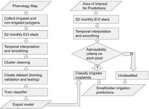
Figure 1. Flowchart of the irrigation detection methodology.

2.1 Phenological characterization

The identification of dry season irrigation stems from the analysis of seasonal vegetation patterns. These patterns occurs in sync with rainfall seasons that are driven by the movement of the Intertropical Convergence Zone (ITCZ). The ITCZ is formed at the thermal equator where the rising air from heat causes a system of low pressure. This facilitates the formation of clouds producing rainfall. The thermal equator is a region that receives intense heat from the sun and migrates latitudinally across the Sahel as the earth orbits the sun. This causes shorter wet seasons in the northern parts of the Sahel and no pronounced dry season closer to the equator. This movement of rainfall patterns causes vegetation growth and senescence. Figure 2 presents an illustration of these vegetation patterns in Africa using EVI from MODIS imagery across the calendar year.

Figure 2

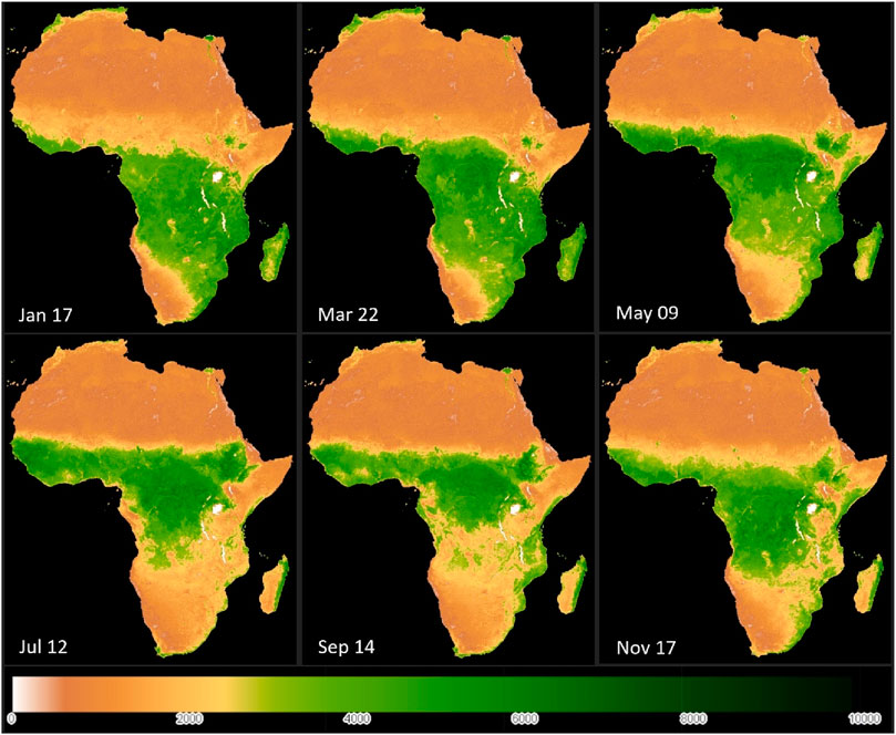
Figure 2. Illustration of vegetation patterns across Africa in 2021 based on MODIS EVI. Certain sub-Sahran geographies are characterized by a prolonged dry season while other regions experience longer rainfall periods as evident by prevalent vegetation across the year.

A phenological characterization of these vegetation patterns can be done by identifying the dominant vegetation cycles called temporal end members (tEMs). Mixture modeling of the temporal end members derived from distinct MODIS 250 m Enhanced Vegetation Index (EVI) time series characterizes native vegetation phenologies at regional scale to provide the basis for a continuous phenology map. Thus each pixel’s EVI time series P_tx (contained in the time space cube with x pixels and t timesteps) can be represented by a linear mixture model (Small, 2012).

${\mathrm{P}}_{tx}={\displaystyle \sum _{i=1}^n}{C}_{ti}{F}_{ix}+{\mathrm{\epsilon }}_{tx}$

s.t. $F_{ix}\ge 0,i=1,...,n$ (non-negativity constraint) and ${\displaystyle \sum _{i=1}^n}{F}_{ix}$ (sum to one constraint)

where:

C_ti are the temporal endmembers.

F_ix are the weights/fractions of each tEM with some residual error Ɛ_tx.

The spatial fractions F_ix can then be mapped to study the vegetation phenologies while the corresponding temporal endmembers represent the phenological cycle associated with each fraction map. Sousa and Small (2022) used the temporal mixture modeling methodology described above to produce a phenology map for the Sahel shown in Figure 3 using MODIS EVI time series (Sousa and Small, 2022). The map is created using four tEMs. Regions dominated by single cropping cycle per year peaking in September are shown in red whereas regions with two cropping cycles per year peaking in May and November are shown in blue. Similarly, regions with prevalent evergreen vegetation are represented with green and barren areas are shown in black. This resembles the agroecological map of Africa (Wilkus et al., 2019) and forms a basis to characterize the African landscape.

Figure 3

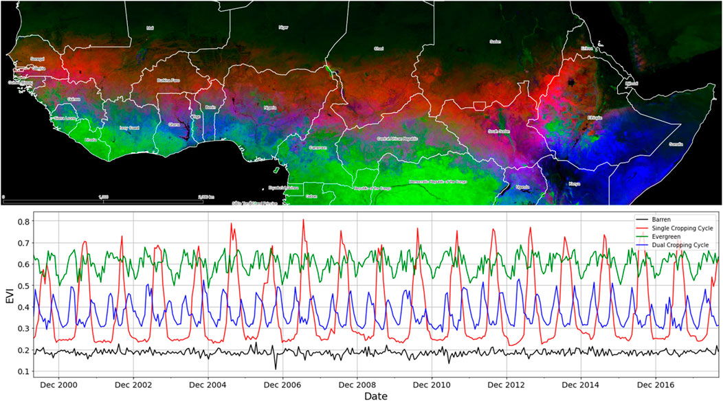
Figure 3. Phenology map of the Sahel created using 18 years of MODIS 500 m imagery at 16 days timesteps by Sousa and Small (2022) and visualized in QGIS. 4 tEMs corresponding to single cropping cycles (red), dual cropping cycles (blue), evergreen (green) and barren/non-vegetated (black) are used for unmixing are plotted.

2.2 Selection of study regions

This phenological characterization is crucial to distinguish our definition of dry season irrigation phenology (an EVI peak is observed in the dry season) from regions with dual cropping cycles. Due to this potential similarity in phenologies, the performance of a classifier trained to detect a dry season peak deteriorates when it is applied to regions with a dual cropping cycle. Therefore, the application of the methodology is restricted to regions with a single cropping cycle (shown in red in Figure 3). Another key challenge emerges when looking at single cropping cycles across different countries in the phenology map of the Sahel. While the northern part of Uganda also has a single cropping cycle, it experiences longer rainfall periods and a shorter dry season. This prompts the need for regional phenology maps to understand if the methodology is applicable across all regions with single cropping cycles.

We hypothesize that the methodology is applicable in semi-arid regions with a prolonged dry season and not applicable in humid regions. To test this hypothesis, we selected study regions consisting of Northern Nigeria, Burkina Faso and Uganda. The northern part of Nigeria which consist of roughly two-fifths of the total area of the country and almost all of Burkina Faso are dominated by a single cropping cycle similar to the Ethiopian Highlands as evident in Figure 3. Uganda experiences longer rainfall periods and is thus more humid. Temporal end members were extracted for each study region to create phenology maps shown in Figure 4. Note that while the use of colors to denote regions with single and dual cropping cycles as well as non-vegetated and evergreen vegetation remains consistent with the phenology map of the Sahel (Figure 3), the vegetation cycle differs across regions. For example, the length of the dry season in regions shown in red in semi-arid areas (Nigeria and Burkina Faso) is 6 months compared to humid areas (Uganda) with a shorter dry season of 3 months. The next step involves collecting labels over our study regions.

Figure 4

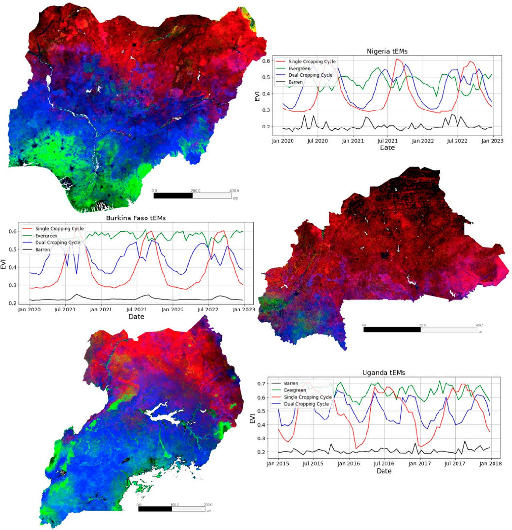
Figure 4. Phenology maps for Nigeria, Burkina Faso and Uganda created using MODIS 250 m imagery are shown with corresponding tEMs in subplots used for mixture modeling. Regions with single cropping cycles per year, dual cropping cycles per year and evergreen regions are shown in red, blue and green channels respectively.

2.3 Label collection

An app built using Google Earth Engine was used to interactively examine the mean Sentinel 2 EVI time series for each polygon drawn over areas of interest through visual inspection of dry season composite and submeter resolution Google Earth imagery. These polygons are either discarded or saved as irrigated/non-irrigated depending on if an EVI peak is observed in the dry season. The dry season for Northern Nigeria based on Figure 4 is taken to be from January 1^st to August 1^st and for Burkina Faso from November 1^st to May 1^st. These dates also are used to create a false color composite of dry season Sentinel 2 imagery with SWIR, NIR and visible blue bands used in the RGB channels. Short wave infrared produces a better contrast between substrate and vegetation compared to the red band. Figure 5 illustrates the process of label collection for a location in Burkina Faso Northeast of Zémpana by the Sourou River. The EVI timeseries for AOIs drawn are shown on the bottom right window for a sample irrigated plot in blue, non-irrigated in red and evergreen in yellow. An EVI peak is evident for the irrigated plot in the dry season window highlighted in green.

Figure 5

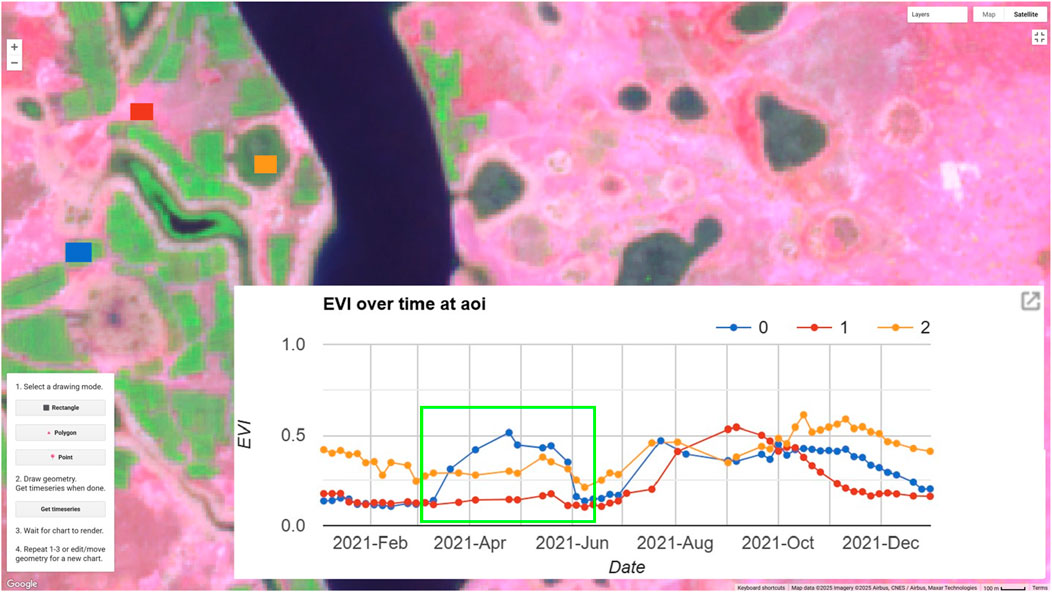
Figure 5. Illustration of visual label collection process in Burkina Faso using an app developed in GEE. An example of irrigated label 0, non-irrigated label 1 and evergreen label 2 (discarded) with the EVI timeseries in blue, red and yellow are shown. A green window highlights the dry season where an EVI peak is observed for irrigated plot.

For the purpose of labeling, each region of interest was split into 10 × 10 km grids. 10% of these are randomly selected to use for labeling. However, this approach of obtaining balanced sampling is not efficient as most of the tiles would not conform to regions containing agriculture. Therefore, a better approach would have been to filter tiles using cropland maps or high-resolution settlement layers. This was not done due to concerns of spatial inconsistency across different study regions among available cropland products (Wei et al., 2020). The labeling effort was also biased towards locating irrigated polygons to ensure a balanced dataset of irrigated and non-irrigated labels as there are significantly more non-irrigated fields versus irrigated fields. This resulted in 197 irrigated and 143 non-irrigated polygons in Nigeria and 129 irrigated and 135 non-irrigated labels in Burkina Faso. Labeling was unfruitful in Uganda due to shorter dry season (insufficient for background vegetation to senesce) and cloud cover issues from longer rainfall periods (A detailed document for labeling used by enumerators is available on Github).

2.4 Cluster cleaning

The labelled polygons were then exported as geojson files and used to generate corresponding temporal stacks of EVI at 10-day timesteps. Since each polygon may cover multiple fields, using the mean of the EVI timeseries of all pixels would mean fields having different crops, planting and harvesting cycles, irrigation techniques and weeds/non-weeds etc., would not be captured. To mitigate this, we use the EVI timeseries of each pixel inside the labelled polygons. These timeseries undergo temporal interpolation and smoothing based on Savitzky Golay filter (order = 3, window size = 60 days) to fill in missing data points and smooth abrupt changes in EVI due to cloud cover, sensor error and other effects. The polygons from both classes are split into training (70%), validation (15%) and testing (15%) and the smoothed timeseries are saved as csvs. Hierarchical Gaussian mixture model is then used for unsupervised clustering of the time series. The clusters are used to examine the vegetation phenologies and remove ones that do not fit in the description of irrigated or non-irrigated. An example of this process for Burkina Faso is shown in Figure 6. Table 1 summarizes the number of pixel time series after cluster cleaning that are then saved as tfrecord files (compressed format for TensorFlow). These are used to train classifiers.

Figure 6

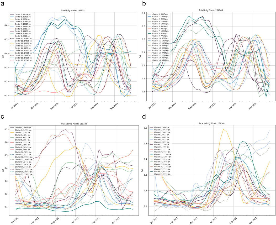
Figure 6. Unsupervised clustering of EVI time series before and after cleaning for irrigated ((a,b) respectively) and non-irrigated pixels (c,d) for Burkina Faso. The clusters that do not fit the definition of irrigated (e.g., cluster 14 in figure (a)) and non-irrigated (e.g., cluster 0 in figure (c)) are removed to prepare the training dataset.

Table 1

Table 1. Summary metrics of data used for training resulting from labeling and cluster cleaning.

2.5 Admissibility criteria

For inference, a temporal stack of EVI at 10-day timesteps is created for regions of interest. These undergo a temporal interpolation smoothing step similar to the one described above for labels. The EVI stack is subjected to rules/admissibility criteria determined by the 90^th and 10^th percentile of EVI. To remove evergreen vegetation, a cutoff on the 10^th percentile of EVI time series that never drop below a certain threshold is applied. Similarly ensuring the 90^th percentile of the EVI time series is greater than the threshold gets rid of barren regions. The threshold was set at 20% of maximum EVI values for Nigeria and Burkina Faso and determined using the tEM plot from Figure 3 (EVI values for the barren tEM is 0.2 or lower). Another condition that the ratio of 90^th and 10^th percentile of EVI timeseries is greater than 2 gets rid of further evergreen pixels. This criterion comes from analysis of the phenology map of the Sahel where the EVI values of the evergreen phenology vary from 0.5 to 0.65 giving a ratio of 1.3 (less than 2). Applying these admissibility criteria reduces the amount of computation required for the classifier which then predicts dry season irrigation and outputs a raster file with binary classification of the predictions.

2.6 Training

Gradient boosted decision trees have continued to dominate as algorithms of choice when it comes to remote sensing classification and detection methodologies (Mooney and Culliton, 2023). However, neural networks with suitable architectures to the task can improve the classification performance often at the expense of computation resources. Conlon et al. (2022) compared random forest classifier, gradient boosted decision trees, and 3 neural network architectures (baseline, LSTM and transformer based networks). The transformer model outperformed all other models followed closely by the catboost model. This study uses the same transformer model architecture shown in Figure 7 to detect smallholder irrigation in Northern Nigeria and Burkina Faso. The model consists of 50,010 trainable parameters, uses an Adam Optimizer with a learning rate of 0.001 and a binary cross entropy loss function. Class balancing weights that are inversely proportional to their class frequency are used to address imbalances in the number of irrigated and non-irrigated training samples. A batch size of 64 with 30 epochs is used for training done on the Google Cloud Platform using a VM instance comprising of n1-standard-8 (8 vCPUs, 30 GB Memory) and one NVIDIA Tesla P4 GPU.

Figure 7

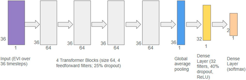
Figure 7. Transformer Model architecture showing the encoding blocks used for predictions.

2.7 Inference

The Food and Agriculture Organization of the United Nations provides statistics for areas equipped for irrigation and maps with irrigated areas as a fraction of the areas equipped for irrigation (AQUAMAPS, 2013). The FAO-Aquastat statistics are based on estimates, land cover maps, public irrigation schemes, fadama schemes and river basin development authorities. A breakdown of the methods utilized to determine irrigated area for each country is reported (Siebert et al., 2013). While these maps are dated and report irrigation infrastructure, the hypothesis is that a comparison of the predictions at state level as a fraction of total cropland area that is irrigated can illustrate the agreement of the classifications with the reported statistics.

3 Results

The classifier achieves an overall F1 score ($\frac{\mathrm{T}\mathrm{P}}{\mathrm{T}\mathrm{P}+0.5\left(\mathrm{F}\mathrm{P}+\text{FN}\right)}$) of more than 96% on the withheld testing dataset across both countries. Table 2 presents a breakdown of the training metrics including true positives (TP) and negatives (TN) as well as false positives (FP) and negatives (FN).

Table 2

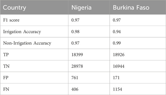
Table 2. Transformer model training metrics for Nigeria and Burkina Faso on the withheld testing dataset.

3.1 Northern Nigeria

Roughly two-fifths of Northern Nigeria has a prolonged dry season where dry season irrigation is easy to detect and receives annual rainfall below 700 mm. The Southern part of Nigeria experiences an average annual rainfall of 2000 mm. The central region is characterized by two rainfalls during the year and receives 1200 mm or less. Most of the irrigation in Nigeria takes place in the Fadamas which are irrigated flood plains across major river valleys, river Niger and river Benue (Eduvie and Garba, 2021). Shallow aquifers are constantly recharged through flash flooding and hold groundwater for dry season irrigation. The majority of the fadamas lie in the Sokoto River basin with minor famadas in sedimentary terrain in Kaduna, Karami, Galma, Kachia, Tubo, Kuri, etc. (Xie et al., 2017). Identifying these areas, presents an opportunity for mechanization through introduction of irrigation technologies and identifying productive uses of energy such agro-processing and cold storage.

Figure 8 shows the irrigation predictions for Northern Nigeria. Parts of Kano, Jigawa and Bauchi are zoomed in at the top. The outlines of AQUASTAT tiles containing irrigation infrastructure are shown in white to assess the spatial correlation with the predictions in yellow. An example of smallholder dry season irrigation south of Gusau is zoomed in at the bottom against high-resolution Google Earth imagery of the region on the right. Two polygons are drawn to verify the irrigated predictions in blue and non-irrigated in red. An EVI peak is observed in the dry season for the irrigated field highlighted by a green window.

Figure 8

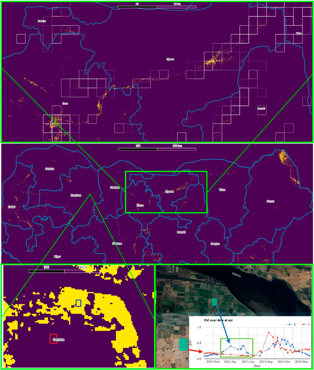
Figure 8. Irrigation Predictions in Northern Nigeria for 2021. Areas predicted to have dry season irrigation appear as yellow on the map. Total land area that the classifiers were used to predict over is roughly 400000 km². Less than 1% of the total area is predicted to be irrigated. FAO AQUASTAT tiles in white are used to assess spatial correlation with predictions in the zoomed in states at the top. An area near Gusau is zoomed in at the bottom to show predictions against sub-meter resolution imagery and polygons drawn to verify the predictions.

A state by state comparison between the cropland area that is predicted to be irrigated is plotted against the percentage of cropland area that is equipped for irrigation from AQUASTAT in Figure 9. The area predicted to be irrigated agrees with the FAO statistics on areas equipped for irrigation except Zamfara, Yobe and Borno where the predicted area that is irrigated is less than that equipped for irrigation. The outlier states suggest an underutilization of irrigation potential because the area predicted to be irrigated is less than the area equipped for irrigation.

Figure 9

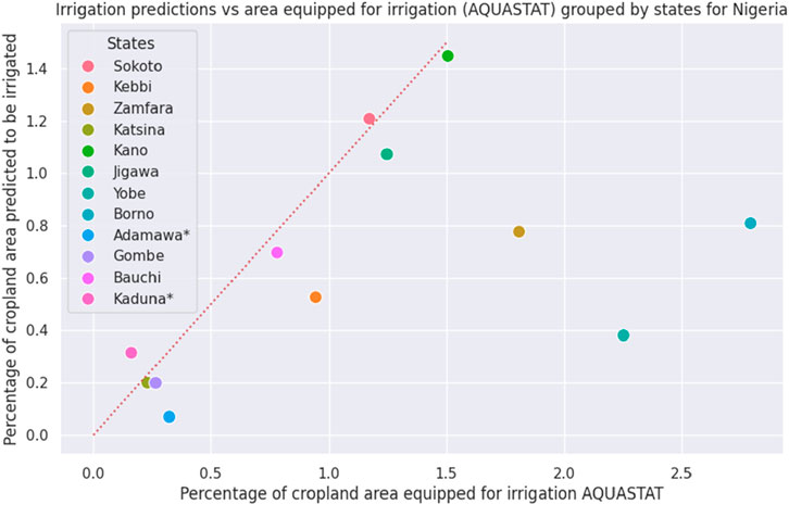
Figure 9. Plot of percentage of cropland area predicted to be irrigated vs. percentage of cropland area equipped for irrigation from AQUASTAT by state. A 1:1 (y = x) line is plotted as a red dotted line.

3.2 Burkina Faso

Burkina Faso which is landlocked by the Sahara Desert to the North and the Gulf of Guinea to the South. Most of the country experiences prolonged dry season which makes dry season irrigation easier to detect. The rainy season lasts from May to September and the dry season occurs in the winter from October to April. The annual rainfall fluctuates between 500 mm in the North to 900 mm and over in the South. Gravity fed irrigation is practiced with water diverted from rivers using feeder canals (Dembele et al., 2012). Figure 10 shows irrigation predictions for Burkina Faso.

Figure 10

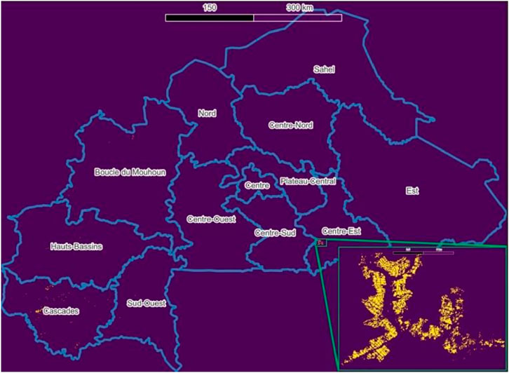
Figure 10. Irrigation Predictions in Burkina Faso for 2021. Areas predicted to have dry season irrigation appear as yellow on the map. Only 113 sqkm of irrigation is found across the entire Burkina Faso. An irrigation scheme in Centre-Est region of Burkina Faso in 2021 is shown zoomed in.

The percentage of cropland area that is predicted to be irrigated is plotted against the percentage of cropland area that is equipped for irrigation from AQUASTAT by State in Figure 11. A general agreement is observed except for Hauts-Bassins where the cropland area predicted to be irrigated is lower than the cropland area equipped for irrigation.

Figure 11

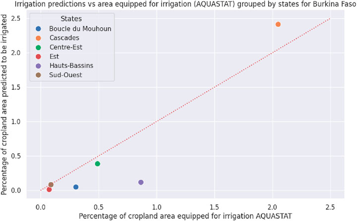
Figure 11. Plot of percentage of cropland area predicted to be irrigated vs. percentage of cropland area equipped for irrigation from AQUASTAT by state. States with no predicted irrigation have been omitted from the plot. A 1:1 (y = x) line is plotted as a red dotted line.

3.3 Uganda

Uganda receives more rainfall throughout the year ranging from 700 mmm to 1500 mm leading to a shorter dry season than other parts of the Sahel such as Ethiopia that have a prolonged dry season. This is reflected in the phenology map of Uganda in Figure 4 where the single cropping cycle represented in the red channel has a dry season that lasts for 3 months from January to March. In comparison, the prolonged dry seasons observed in Northern Nigeria and Burkina Faso last for 6 months of the year. Fewer cloud-free images are available due to longer rainfall periods resulting in noisier EVI time series. The absence of a pronounced dry season obstructs the identification of croplands that exhibit a non-perennial vegetation cycle in the dry season since the surrounding vegetation hasn’t had ample time to senesce.

Columbia World Projects carried out a survey including farmer interviews in Uganda during the dry season months of early 2023 (Modi, 2025). Some of the smallholder farms had the smaller side length of the plots less than the 10 m pixel resolution of Sentinel 2 making vegetation patterns harder to detect due to mixed pixels. Several farmers tend to grow multiple crops within their agriculture plot which is aimed at serving subsistence farming needs. Proper irrigation knowledge and resources are either limited or absent (Hortirrigation, 2025). The survey was aimed at interviewing farmers that irrigate resulting in a biased dataset of 11,021 interviews of farmers that irrigate and 3,818 farmers that don’t. The data revealed that 88% of the farmers in Uganda use manual irrigation methods with handheld containers accounting for 85% of the water transportation to the fields. Identification of these farmers is an opportunity for targeted investment in infrastructure, introduction of irrigation technologies, and development of supply chains and markets. EVI timeseries were extracted for each plot coordinate obtained from the survey. This was used to assess classifier performance trained on phenology as labelling efforts in this region were unfruitful due to the challenges described earlier. The transformer F1 scores on the withheld testing data deteriorated to 62% over irrigated areas (TP: 777, TN: 630, FP: 412, FN: 540) as opposed to 96% achieved in Nigeria and Burkina Faso.

Figure 12 shows a comparison of the mean, 25th and 75th percentiles of Sentinel-2 EVI time series for different plots across the Ethiopian Highlands from Conlon et al. (2022), Northern Nigeria, Burkina Faso and surveyed sites in Uganda. The EVI timeseries for Uganda were extracted for farmer plot locations from the interviews. While the other regions exhibit a distinct peak in the dry season for irrigated time series, no clear distinction is observed for the different plots in Uganda among irrigated and non-irrigated EVI time series.

Figure 12

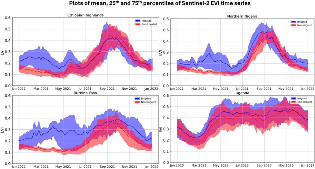
Figure 12. Plots of mean, 25th and 75th percentiles of Sentinel-2 EVI time series for multiple plots across the Ethiopian Highlands, Northern Nigeria, Burkina Faso and Uganda are shown.

4 Discussion

Knowing the locations of the smallholder farmers that irrigate is essential for energy access planning in order to size the grids to meet the demand associated with irrigation and agro-processing and thus understand the associated costs. Therefore from developer perspective, the essential question is related to the probability that a 10 m × 10 m pixel which corresponds to 0.01 hectare area of land is actually irrigated given that the classifier predicts it to be irrigated.

Given that we can obtain prior knowledge of irrigation through FAO Aquastat, this can be worked out using the Bayes Theorem. In Kano, 1.3% of the total area is equipped for irrigation. The probability that a given pixel is irrigated is 0.013 and not irrigated is 0.987. Table 2 provides the Transformer model performance metrics for Nigeria. The true positives is the probability that the classifier gives a positive result (predicts irrigated) given that the test label is irrigated which is 0.96. Similarly the true negatives is the probability that the classifier gives a positive result (predicts irrigated) given that the test label is irrigated which is 0.014. Therefore the probability that a 10 m × 10 m pixel in Kano is actually irrigated given that the model predicts it to be irrigated is 0.48.

Having more than one irrigated pixel or clusters of smallholder irrigation increases the probability that the pixels predicted to be irrigated are actually irrigated. Therefore the results were then aggregated to 250 m × 250 m which corresponds to 6.25 ha and binned into categories of fraction of the 250 m × 250 m pixel that is irrigated. This can be used as a prior to increase the probability of targeting areas that are irrigated given that they are classified as irrigated. The predictions are uploaded to CWP dashboard (can be viewed under the “Map” tab by navigating to the “landscape predictions and analysis” drop down menu and toggling the “N.Nigeria: % area predicted irrigated (6.25ha)” layer). The dashboard is a platform that hosts raster and vector layers related to energy for productive use projects, a Columbia World Projects initiative carried out by Quadracci Sustainable Engineering Laboratory (Columbia, 2025).

5 Conclusion

Mapping irrigated areas has vital policy implications for supporting economic growth through irrigation development. It is also key to achieving the United Nation’s Sustainable Development Goals (SDGs) namely, alleviating food insecurity (SDG 2), sustainable management of water resources (SDG 6) and adapting agriculture to climate change (SDG 13). The energy required for pumping water for irrigation and associated productive uses of energy (PUEs) such as agro-processing provide flexible load integration to household demand. This load shifting flexibility offers system benefits for sustainable and economically viable energy access solutions.

Dry Season photosynthetic growth can be identified using dry season false color composites to get a stark contrast between vegetation and substrate. The challenge then becomes to separate the different classes such as evergreen vegetation like forests, rainfed-crops, swamps, etc. from dry-season irrigated agriculture. The temporal profile of vegetation indices such as EVI provides information about crop growth, maturity and senescence. If these occur during the dry season with no rainfall to meet crop water requirements, it indicates the use of irrigation techniques. This is however dependent on the climate and the landscape being examined. In humid areas with longer rainfall periods, the surrounding vegetation that relies on rainfall does not senesce due to the absence of a pronounced dry season. Therefore, dry season irrigation in these regions cannot be differentiated from rain-fed agriculture and other prevalent vegetation types such as shrubs, grasslands, etc. Thus a prolonged dry season (lasting for at least 6 months as shown in the examples in Figure 12) is paramount for these classifiers to identify smallholder farms that irrigate during the dry season.

The methodology developed to detect dry season irrigation in the Ethiopian highlands was operationalized to detect smallholder irrigation in Northern Nigeria and Burkina Faso to demonstrate the scope of the classifier. Other semi-arid regions with a similar prolonged dry season where the methodology could be applicable include countries such as Senegal, Mali, Ghana, etc. Even though the comparative analysis was limited to the Sahel, the methodology is likely applicable to countries south of the equator such as Malawi which have a pronounced dry season. These conform with the semi-arid regions in the agroecological map of Africa.

Humid areas such as Uganda with shorter dry seasons require a different approach to identify smallholder irrigation. This may be accomplished through a traditional machine learning approach incorporating features such as topography maps, precipitation, evapotranspiration, distance to surface water, distance to infrastructure, etc. to understand where the farmers choose to irrigate (Walsh et al., 2023).

Unmanned Aerial Vehicles have often been utilized to overcome barriers of spatial resolution and provide sub-meter resolution imagery (Nhamo et al., 2020) (Cucho-Padin et al., 2020). While these are essential for crop classification, the characterization of irrigation is reliant on temporal data to distinguish the vegetation cycle from non-irrigated agriculture that might not be available through UAVs.

Data availability statement

The scripts (Google Earth Engine and Google Collab), training data and trained models used for the results in this paper are available on Github at github.com/hssiddiqui/Irrigation-Detection-SSA. The repository also contains supplementary documentation such as instructions for label collection.

Author contributions

HS: Investigation, Writing – original draft, Formal Analysis, Data curation, Visualization, Validation, Conceptualization. CS: Supervision, Writing – review and editing. VM: Writing – review and editing, Funding acquisition, Supervision.

Funding

The author(s) declare that financial support was received for the research and/or publication of this article. Partial support for this effort was provided by the National Science Foundation (INFEWS Award Number 1639214), Columbia World Projects, Rockefeller Foundation (eGuide Grant 2018POW004), OPML United Kingdom (DFID) and Technoserve (BMGF).

Acknowledgments

The authors would like to acknowledge Terence Conlon’s efforts in development of the original methodology in Descartes Labs Platform and comparison of the different classifiers. The authors would like to thank Vlad Pyltsov, Imad Heit and the Taqadem team for help with labeling, Emily Logan and Priya Suresh at Atlas AI for help with the Google Earth Engine Platform, Edwin Adkins and Markus Walsh for their guidance with surveys and remote sensing features.

Conflict of interest

The authors declare that the research was conducted in the absence of any commercial or financial relationships that could be construed as a potential conflict of interest.

The author(s) declared that they were an editorial board member of Frontiers, at the time of submission. This had no impact on the peer review process and the final decision.

Generative AI statement

The author(s) declare that no Generative AI was used in the creation of this manuscript.

Any alternative text (alt text) provided alongside figures in this article has been generated by Frontiers with the support of artificial intelligence and reasonable efforts have been made to ensure accuracy, including review by the authors wherever possible. If you identify any issues, please contact us.

Publisher’s note

All claims expressed in this article are solely those of the authors and do not necessarily represent those of their affiliated organizations, or those of the publisher, the editors and the reviewers. Any product that may be evaluated in this article, or claim that may be made by its manufacturer, is not guaranteed or endorsed by the publisher.

References

Angelakιs, A. N., Zaccaria, D., Krasilnikoff, J., Salgot, M., Bazza, M., Roccaro, P., et al. (2020). Irrigation of World agricultural lands: evolution through the millennia. Water 12 (5), 1285. doi:10.3390/w12051285

CrossRef Full Text | Google Scholar

AQUAMAPS (2013). global spatial database on water and agriculture. Available online at: https://data.apps.fao.org/aquamaps (Accessed: September. 03, 2023).

Google Scholar

Azzari, G., and Lobell, D. B. (2017). Landsat-based classification in the cloud: an opportunity for a paradigm shift in land cover monitoring. Remote Sens. Environ. 202, 64–74. doi:10.1016/j.rse.2017.05.025

CrossRef Full Text | Google Scholar

Bjornlund, V., Bjornlund, H., and Van Rooyen, A. (2022). Why food insecurity persists in sub-Saharan Africa: a review of existing evidence. Food secur. 14 (4), 845–864. doi:10.1007/s12571-022-01256-1

PubMed Abstract | CrossRef Full Text | Google Scholar

J. A. Cardille, M. A. Crowley, D. Saah, and N. E. Clinton (2024). Cloud-based remote sensing with google earth engine: fundamentals and applications (Cham: Springer International Publishing). doi:10.1007/978-3-031-26588-4

CrossRef Full Text | Google Scholar

Columbia (2025). Columbia World projects energy for productive use. Available online at: https://qsel.columbia.edu/cwp-epu-data-platform/.

Google Scholar

Conlon, T., Small, C., and Modi, V. (2022). A multiscale spatiotemporal approach for smallholder irrigation detection. Front. Remote Sens. 3, 871942. doi:10.3389/frsen.2022.871942

CrossRef Full Text | Google Scholar

Cucho-Padin, G., Loayza, H., Palacios, S., Balcazar, M., Carbajal, M., and Quiroz, R. (2020). Development of low-cost remote sensing tools and methods for supporting smallholder agriculture. Appl. Geomat. 12 (3), 247–263. doi:10.1007/s12518-019-00292-5

CrossRef Full Text | Google Scholar

Dembele, Y., Yacouba, H., Keïta, A., and Sally, H. (2012). Assessment of irrigation system performance in south western Burkina Faso. Irrig. Drain. 61 (3), 306–315. doi:10.1002/ird.647

CrossRef Full Text | Google Scholar

Eduvie, M. O., and Garba, M. L. (2021). Appraisal of groundwater potential of fadama areas within northern Nigeria: a review. J. Geosci. Environ. Prot. 09 (03) 44–57. doi:10.4236/gep.2021.93004

CrossRef Full Text | Google Scholar

FAO (2019). “Moving forward on food loss and waste reduction,” in The state of food and agriculture, no. 2019 (Rome: Food and Agriculture Organization of the United Nations).

Google Scholar

Hortirrigation (2025). Participatory research and development with smallholder farmers in Uganda to improve small-scale irrigation. Innovations Dry Seas. Hortic. Available online at: https://www.hortirrigation.org/.

Google Scholar

Kocaman, A. S., Ozyoruk, E., Taneja, S., and Modi, V. (2020). A stochastic framework to evaluate the impact of agricultural load flexibility on the sizing of renewable energy systems. Renew. Energy 152, 1067–1078. doi:10.1016/j.renene.2020.01.129

CrossRef Full Text | Google Scholar

Magidi, J., Nhamo, L., Mpandeli, S., and Mabhaudhi, T. (2021). Application of the random forest classifier to map irrigated areas using google earth engine. Remote Sens. 13 (5), 876. doi:10.3390/rs13050876

PubMed Abstract | CrossRef Full Text | Google Scholar

Modi, V. (2025). Livelihoods, M300/ASCENT, and small-holder irrigation- case study from Uganda. Available online at: https://qsel.columbia.edu/cwp-briefs-3/.

Google Scholar

Mooney, P., and Culliton, P. (2023). Kaggle AI report 2023. Available online at: Kaggle.com.

Google Scholar

Muzammal, H., Zaman, M., Safdar, M., Shahid, M. A., Sabir, M. K., Khil, A., et al. (2024). “Climate change impacts on water resources and implications for agricultural management,” in Transforming agricultural management for a sustainable future. Editors S. Kanga, S. K. Singh, K. Shevkani, V. Pathak, and B. Sajan (Cham: Springer Nature Switzerland), 21–45. doi:10.1007/978-3-031-63430-7_2

CrossRef Full Text | Google Scholar

Nhamo, L., Magidi, J., Nyamugama, A., Clulow, A. D., Sibanda, M., Chimonyo, V. G. P., et al. (2020). Prospects of improving agricultural and water productivity through unmanned aerial Vehicles. Agriculture 10 (7), 256. doi:10.3390/agriculture10070256

CrossRef Full Text | Google Scholar

Ozdogan, M., Yang, Y., Allez, G., and Cervantes, C. (2010). Remote sensing of irrigated agriculture: opportunities and challenges. Remote Sens. 2 (9), 2274–2304. doi:10.3390/rs2092274

CrossRef Full Text | Google Scholar

Rufin, P., Frantz, D., Ernst, S., Rabe, A., Griffiths, P., Özdoğan, M., et al. (2019). Mapping cropping practices on a national scale using intra-annual Landsat time series binning. Remote Sens. 11 (3), 232. doi:10.3390/rs11030232

CrossRef Full Text | Google Scholar

Siddiqui, H., and Modi, V. (2024). “Monitoring the impacts of disruption events on agriculture through irrigation detection with remote sensing,” in 2024 IEEE Global Humanitarian Technology Conference (GHTC), Radnor, PA, USA (IEEE), 286–291. doi:10.1109/GHTC62424.2024.10771556

CrossRef Full Text | Google Scholar

Siebert, S., Henrich, V., Frenken, K., and Burke, J. (2013). Update of the digital global map of irrigation areas to version 5. doi:10.13140/2.1.2660.6728

CrossRef Full Text | Google Scholar

Small, C. (2012). Spatiotemporal dimensionality and Time-Space characterization of multitemporal imagery. Remote Sens. Environ. 124, 793–809. doi:10.1016/j.rse.2012.05.031

CrossRef Full Text | Google Scholar

Sousa, D., and Small, C. (2022). Joint characterization of spatiotemporal data manifolds. Front. Remote Sens. 3, 760650. doi:10.3389/frsen.2022.760650

CrossRef Full Text | Google Scholar

Vogels, M., De Jong, S., Sterk, G., Douma, H., and Addink, E. (2019). Spatio-temporal patterns of smallholder irrigated agriculture in the horn of Africa using GEOBIA and sentinel-2 imagery. Remote Sens. 11 (2), 143. doi:10.3390/rs11020143

CrossRef Full Text | Google Scholar

Walsh, M., Modi, V., and Siddiqui, H. (2023). Stacked spatial predictions of smallholder irrigation in Uganda. Available online at: https://africasoils.info/wp-content/uploads/2023/12/Uganda_irrigation_prediction.html.

Google Scholar

Wei, Y., Lu, M., Wu, W., and Ru, Y. (2020). Multiple factors influence the consistency of cropland datasets in Africa. Int. J. Appl. Earth Obs. Geoinformation 89, 102087. doi:10.1016/j.jag.2020.102087

CrossRef Full Text | Google Scholar

Wilkus, E., Roxburgh, C., and Rodriguez, D. (2019). Understanding household diversity in rural eastern and southern Africa aciar monograph 205.

Google Scholar

Xie, H., You, L., and Takeshima, H. (2017). Invest in small-scale irrigated agriculture: a national assessment on potential to expand small-scale irrigation in Nigeria. Agric. Water Manag. 193, 251–264. doi:10.1016/j.agwat.2017.08.020

CrossRef Full Text | Google Scholar