Practical aspects of providing pixel-level spectral Rrs error covariance in satellite ocean color products

We previously established a derivative-based approach to generate a pixel-level spectral error covariance matrix in satellite-retrieved remote sensing reflectance, ∑R_rs. However, one practical issue is the delivery of the products without increasing the file size by an order of magnitude or more, considering that for N sensor spectral bands, there are N × (N+1)/2 covariance matrix elements to be specified at each pixel. The issue becomes more pertinent for hyperspectral imaging spectroradiometers such as the Ocean Color Instrument (OCI) on NASA’s Plankton, Aerosol, Cloud, ocean Ecosystem mission (PACE), which has 286 bands, resulting in ∼40,000 unique elements in ∑R_rs per pixel that would lead to a ∼60 GB Level-2 file for one 5-min granule. As a first step to tackle the issue, we took OCI and Moderate Resolution Imaging Spectroradiometer (MODIS) data to explore the possibility of approximating ∑R_rs using a third-degree polynomial, thereby decreasing the memory overhead to 4×N numbers. We found that ∑R_rs derived from the polynomial fitting matches well with the original value, with the difference smaller than 5%. We then compared the relative uncertainty in two derived ocean color data products (chl_a and K_d(490)) calculated using the original fully computed ∑R_rs and then using the polynomial model approximation for ∑R_rs, finding the absolute difference between the two approaches to be smaller than 0.5%. These evaluations suggest the polynomial approximation of ∑R_rs is suitable without degrading the scientific quality. By including the coefficients derived from polynomial fitting instead of the full error covariance matrix, a typical 5-min Level-2 file for OCI decreases from ∼60 GB to a more practical ∼1.7 GB.

1 Introduction

Due to the capability of obtaining a long time series of data at a global scale, satellite remote sensing has been widely used to study Earth System science and global change (Dutkiewicz et al., 2019; Cael et al., 2023). As a product fundamental to deriving a host of bio-optical and biogeochemical properties of the water column, ocean remote sensing reflectance (R_rs, sr⁻¹) has been routinely generated from satellite radiometry and distributed by NASA’s Ocean Biology Distributed Active Archive Center (OB.DAAC) for more than 3 decades. While R_rs and properties derived from it have been validated against ground truth, there is no routinely generated pixel-level uncertainty product. Although the uncertainty in water-leaving reflectance at the pixel level is provided for the Ocean and Land Colour Instrument (OLCI) onboard Sentinel-3 (Lamquin et al., 2013), it is underestimated, as only sensor noise is included. It should be noted that the European Space Agency’s Ocean Color Climate Change Initiative program (OC_CCI) does provide pixel-level uncertainty in R_rs (Jackson et al., 2017), computed using the weighted average of the uncertainty within optical water classes associated with that pixel. The uncertainty of each class is derived from validation against ground truth, which has an issue with representing the pixel-level uncertainty, as described by Zhang et al. (2022). Furthermore, this approach could not capture spatiotemporal variations in some key drivers of uncertainty in R_rs, such as geometry and atmospheric turbidity. Without associated uncertainty, ocean color data products are incomplete measurements, limiting the interpretation of subtle changes in global ocean biology and biogeochemistry. Uncertainty in ocean color products has been recommended by the Group on Earth Observations (GEO) and the International Ocean Colour Coordinating Group (IOCCG) within the framework of quality assurance for earth observation and should be required by any satellite mission (Fox, 2010; IOCCG, 2019).

Historically, the ocean color community has relied on comparison with collocated in situ data to estimate uncertainty in ocean color products via “matchup” validation analyses. While the validation generates reasonable confidence in those products, it has some limitations (Zhang et al., 2022). In addition, while an analytical framework for estimating standard uncertainties in derived biogeochemical data products has been developed (McKinna et al., 2019), implementing this operationally requires pixel-level knowledge of standard uncertainties in R_rs(λ) and the error covariance between R_rs at different bands. Because of these limitations, we developed a derivative-based approach to calculate the pixel-level standard uncertainty in R_rs(λ) retrieved from the Moderate-Resolution Imaging Spectroradiometer (MODIS) aboard Aqua using a multiple scattering epsilon (MSEPS) atmospheric correction algorithm (Ahmad and Franz, 2015), which has been used recently to complete a multi-mission ocean color reprocessing for heritage sensors by the Ocean Biology Processing Group (OBPG) at NASA. The R_rs(λ) uncertainty products generated by Zhang et al. (2022) and Zhang et al. (2024) were demonstrated to be reliable through evaluation using the Monte Carlo method as well as closure analysis with the statistics derived from validation.

While uncertainty can be readily generated, one practical issue is the delivery of all spectral uncertainty products without increasing data file sizes by an order of magnitude or more. A spectral error covariance matrix, ∑R_rs, is necessary. This matrix contains the variance in R_rs(λ_i) at the ith band as the diagonal elements and the covariance between R_rs at the ith and jth band, denoted as u(R_rs(λ_i), R_rs(λ_j)), as the off-diagonal elements. We note the off-diagonal terms in ∑R_rs are not negligible (Zhang et al., 2024) and must be considered when more than one band is used to derive data products, for example, the band ratio algorithms for chlorophyll-a pigment concentration (chl_a, mg/m³) or the diffuse attenuation coefficient for downwelling irradiance at 490 nm (K_d(490), m⁻¹).

Taking MODIS, for example, with N = 10 sensor spectral bands spanning 412 nm −678 nm, ∑R_rs has a dimension of 10 × 10. Considering that ∑R_rs is symmetric, a total of 55 (N × (N+1)/2) numbers must be stored at each pixel. The issue becomes more pertinent as we move forward to hyperspectral sensors with hundreds of bands, such as the Ocean Color Instrument (OCI), with 286 bands ranging from ultraviolet to shortwave infrared wavelengths on NASA’s Plankton, Aerosol, Cloud, ocean Ecosystem mission (PACE) (https://pace.oceansciences.org/about.htm), which launched in February 2024. It is unfeasible to deliver tens of thousands of ∑R_rs values at each pixel, given the broad (∼2,600 km) swath and moderate (1.2 km at the sub-satellite point) spatial footprint. As a first step toward delivering uncertainty products without unmanageably increasing the data file size, we investigate in this study the spectral variation of ∑R_rs retrieved from MODIS and OCI data using the MSEPS algorithm, with the goal of decreasing the dimensionality needed to reproduce it well enough for downstream scientific use.

2 Satellite data

Level-1A (uncalibrated) data of MODIS aboard the Aqua satellite and Level-1B (calibrated and geolocated) data of OCI from the PACE mission were downloaded from the Ocean Biology Distributed Active Archive Center (OB.DAAC). Level-1A MODIS data were processed to Level-1B using the SeaDAS software package (https://seadas.gsfc.nasa.gov) and the latest instrument calibration coefficients, which are also distributed by OB.DAAC. R_rs(λ) was derived by applying the MSEPS atmospheric correction algorithm to L1B data, and the uncertainty in R_rs(λ) was then calculated using the derivative-based approach established by Zhang et al. (2022). Here, we used MODIS data (i) over the Marine Optical BuoY (MOBY) (Clark et al., 2003) during 2002–2019; (ii) over the U.S. East Coast on 28 January 2012; and (iii) globally during 3–10 December 2019. We used OCI data over the U.S. East Coast on 13 May 2024.

3 Methodology

3.1 MSEPS atmospheric correction

We used MSEPS to calculate R_rs(λ) from spectral top-of-atmosphere (TOA) radiances L_t(λ), which can be expressed as Equation 1 (the spectral term, λ, is omitted for brevity):

$L_{\mathrm{t}}/t_{\mathrm{g}}=L_r+L_{\mathrm{a}}+{t_{\text{vr}}L}_{\mathrm{f}}+{TL}_{\mathrm{g}}+t_{\mathrm{v}}{L}_{\mathrm{w}}(1)$

where t_g(λ) is two-way gas transmittance, L_r(λ) (mW.cm⁻².μm⁻¹.sr⁻¹) is the radiance from scattering by air molecules in the absence of aerosol, L_a(λ) (mW.cm⁻².μm⁻¹.sr⁻¹) is the radiance from scattering by aerosols that also accounts for interactions between air molecules and aerosol scattering, L_f(λ) (mW.cm⁻².μm⁻¹.sr⁻¹) is the radiance from scattering by surface whitecaps, L_g(λ) (mW.cm⁻².μm⁻¹.sr⁻¹) is the sun glint, and t_vr(λ) and t_v(λ) are the diffuse transmittance from surface to sensor with the former only including molecular scattering and the latter including molecular and aerosol scattering. T(λ) is the beam transmittance for the view path. L_f (λ) is calculated using wind speed based on an empirical model (Stramska and Petelski, 2003). A sun glint coefficient is calculated using a statistical model (Cox and Munk, 1954), from which L_g(λ) can be derived (Wang and Bailey, 2001). The calculation of L_a(λ) is detailed by Ahmad and Franz (2015). After removing L_r(λ), L_a(λ), L_f(λ), and T(λ) L_g(λ) from L_t(λ), water-leaving radiance L_w(λ) (mW.cm⁻².μm⁻¹.sr⁻¹) can be derived, and R_rs(λ) is then calculated by normalizing L_w(λ) to downwelling irradiance (the spectral term, λ, is omitted for brevity):

$R_{\text{rs}}=\left(L_{\mathrm{t}}/t_{\mathrm{g}}-L_{\mathrm{r}}-{TL}_{\mathrm{g}}-t_{\text{vr}}{L}_{\mathrm{f}}-L_{\mathrm{a}}\right)f_{\mathrm{b}}/\left(t_{\mathrm{v}}{F}_0{t}_{\mathrm{s}}\cos \left({\mathrm{\theta }}_{\mathrm{s}}\right)\right)(2)$

where f_b is the bidirectional reflectance correction calculated from the model presented by Morel et al. (2002) using chl_a, t_s(λ) is the spectral diffuse transmittance from the Sun to the surface, θ_s is the solar zenith angle, and F₀(λ) (mW.cm⁻².μm⁻¹) is the spectral extraterrestrial solar irradiance accounting for the Earth–Sun distance. F₀ for OCI is calculated from the solar irradiance measurements from the Total and Spectral Solar Irradiance Sensor-1 (TSIS-1) (Coddington et al., 2021). F₀ for MODIS is from Thuillier et al. (2004).

3.2 Error covariance in R_rs

While the approach for calculating the error covariance matrix terms u(R_rs(λ_i), R_rs(λ_j)) is detailed by Zhang et al. (2024), we briefly recap here, taking MODIS as an example. It is based on a derivative approach. Two variables y₁ and y₂ are function of variables x, z, expressed by Equation 3:

$\left\{\begin{array}{c}{y}_1=f_1\left(x_1,x_2,\dots ,x_{\mathrm{n}}\right)\\ y_2=f_2\left(z_1,z_2,\dots ,z_{\mathrm{n}}\right)\end{array}\right.(3)$

error covariance between y₁ and y₂, denoted by u(y₁, y₂), following the convention of (IOCCG, 2019), can be derived from Equation 4:

$u\left(y_1,y_2\right)=\left(\frac{\mathrm{\partial }{f}_1}{\mathrm{\partial }{x}_1},\frac{\mathrm{\partial }{f}_1}{\mathrm{\partial }{x}_2},\dots ,\frac{\mathrm{\partial }{f}_1}{\mathrm{\partial }{x}_{\mathrm{n}}}\right){\left[\begin{array}{ccc}u\left(x_1,z_1\right)& \cdots & u\left(x_1,z_n\right)\\ ⋮& \ddots & ⋮\\ u\left(x_n,z_1\right)& \cdots & u\left(x_n,z_n\right)\end{array}\right]\left(\frac{\mathrm{\partial }{f}_2}{\mathrm{\partial }{z}_1},\frac{\mathrm{\partial }{f}_2}{\mathrm{\partial }{z}_2},\dots ,\frac{\mathrm{\partial }{f}_2}{\mathrm{\partial }{z}_{\mathrm{n}}}\right)}^{\mathrm{T}}(4)$

where u(x_i, z_j) represents the error covariance between variables x_i and z_j, $\frac{\mathrm{\partial }{f}_1}{\mathrm{\partial }{x}_{\mathrm{i}}}$ and $\frac{\mathrm{\partial }{f}_2}{\mathrm{\partial }{z}_{\mathrm{j}}}$ are the partial derivatives of y₁ with respect to x_i and of y₂ with respect to z_j, and T is the transpose operator. u(y₁, y₂) turns to variance when f₁ and f₂ are same, denoted by u²(y₁). u(y₁) is the standard uncertainty (JCGM, 2011). Based on Equations 2,4, u(R_rs(λ_i), R_rs(λ_j)) can be calculated from Equations 5–7:

$u\left(R_{\text{rs}}\left({\mathrm{\lambda }}_{\mathrm{i}}\right),R_{\text{rs}}\left({\mathrm{\lambda }}_{\mathrm{j}}\right)\right)=\frac{\mathrm{\partial }{R}_{\text{rs}}\left({\mathrm{\lambda }}_{\mathrm{i}}\right)}{\mathrm{\partial }{X}_{\mathrm{i}}}{C}_{R_{\text{rs}}}{\left(\frac{\mathrm{\partial }{R}_{\text{rs}}\left({\mathrm{\lambda }}_{\mathrm{j}}\right)}{\mathrm{\partial }{X}_{\mathrm{j}}}\right)}^{\mathrm{T}}(5)$

where

$\frac{\mathrm{\partial }{R}_{\text{rs}}\left({\mathrm{\lambda }}_{\mathrm{i}}\right)}{\mathrm{\partial }{X}_{\mathrm{i}}}=\left(\frac{\mathrm{\partial }{R}_{\text{rs}}\left({\mathrm{\lambda }}_{\mathrm{i}}\right)}{\mathrm{\partial }{L}_{\text{rfc}}\left({\mathrm{\lambda }}_{\mathrm{i}}\right)},\frac{\mathrm{\partial }{R}_{\text{rs}}\left({\mathrm{\lambda }}_{\mathrm{i}}\right)}{\mathrm{\partial }{L}_{\text{rfc}}\left(\text{NIR}\right)},\frac{\mathrm{\partial }{R}_{\text{rs}}\left({\mathrm{\lambda }}_{\mathrm{i}}\right)}{\mathrm{\partial }{\text{chl}}_{\mathrm{a}}},\frac{\mathrm{\partial }{R}_{\text{rs}}\left({\mathrm{\lambda }}_{\mathrm{i}}\right)}{\mathrm{\partial }{\mathrm{\tau }}_{\mathrm{a}}^{\prime }\left(869\right)},\frac{\mathrm{\partial }{R}_{\text{rs}}\left({\mathrm{\lambda }}_{\mathrm{i}}\right)}{\mathrm{\partial }rh}\right)(6)$

and

$C_{R_{\text{rs}}}=\left[\begin{array}{ccccc}u\left(L_{\text{rfc}}\left({\mathrm{\lambda }}_{\mathrm{i}}\right),L_{\text{rfc}}\left({\mathrm{\lambda }}_{\mathrm{j}}\right)\right)& u\left(L_{\text{rfc}}\left({\mathrm{\lambda }}_{\mathrm{i}}\right),L_{\text{rfc}}\left(\text{NIR}\right)\right)& 0& 0& 0\\ u\left(L_{\text{rfc}}\left(\text{NIR}\right),L_{\text{rfc}}\left({\mathrm{\lambda }}_{\mathrm{j}}\right)\right)& u^2\left(L_{\text{rfc}}\left(\text{NIR}\right)\right)& 0& 0& 0\\ 0& 0& u^2\left({\text{chl}}_{\mathrm{a}}\right)& 0& 0\\ 0& 0& 0& u^2\left({\mathrm{\tau }}_{\mathrm{a}}^{\prime }\left(869\right)\right)& 0\\ 0& 0& 0& 0& u^2\left(rh\right)\end{array}\right](7)$

X_i is a vector of the uncertainty variables that are used to propagate the uncertainty through the atmospheric correction procedure, which is defined as Equation 8:

$X_{\mathrm{i}}=\left[{L_{\text{rfc}}\left({\mathrm{\lambda }}_{\mathrm{i}}\right),L}_{\text{rfc}}\left(\text{NIR}\right),{\text{chl}}_{\mathrm{a}},{\mathrm{\tau }}_{\mathrm{a}}^{\prime }\left(869\right),rh\right](8)$

where NIR corresponds to the two near-infrared bands used for MSEPS, ${\mathrm{\tau }}_{\mathrm{a}}^{\prime }$ is the aerosol optical thickness, and rh is the relative humidity. L_rfc is defined as Equation 9 (the spectral term, λ, is omitted for brevity):

$L_{\text{rfc}}=L_{\mathrm{t}}/t_{\mathrm{g}}-L_{\mathrm{r}}-t_{\text{vr}}{L}_{\mathrm{f}}(9)$

3.3 Polynomial fitting of spectral u(R_rs(λ_i), R_rs(λ))

Spectral u(R_rs(λ_i), R_rs(λ_j)) are analyzed by fitting u(R_rs(λ_i), R_rs(λ)) as a function of wavelength. Here, λ_i and λ represent a specific wavelength and all the wavelengths, respectively. For example, u(R_rs(412), R_rs(λ)) is fitted as a function of MODIS bands in the wavelength range of 412–678 nm. Only visible wavelengths are considered in this study. We noted previously that the covariance was often spectrally smooth and decayed as a function of wavelength difference (Zhang et al., 2024). As a result, we experimented using a third-degree polynomial:

$u\left(R_{rs}\left({\mathrm{\lambda }}_i\right),R_{rs}\left(\mathrm{\lambda }\right)\right)=\mathrm{a}+\mathrm{b}\lambda +\mathrm{c}{\mathrm{\lambda }}^2+d{\mathrm{\lambda }}^3(10)$

where λ is the central wavelength in units of μm. As the matrix is symmetric, we do not “re-use” wavelengths when fitting polynomials as this will lead to an asymmetry. There are, therefore, ten points used to fit the coefficients for 412 nm (λ = 412, 443, 469, 488, 531, 547, 555, 645, 667, and 678), nine for 443 nm, eight for 469 nm, and so on. This means that there is no need to fit coefficients for wavelengths of 555 nm or longer, considering that there are four or fewer covariances to use for this band, which is equal to or less than the four coefficients needed for the fitting (so it is more efficient to reproduce the matrix exactly). The same fitting method is also applied to OCI. The coefficients a, b, c, and d in Equation 10, derived by means of least-square fitting, are stored in the Level-2 file for each band λ_i.

3.4 Uncertainty in chl_a and K_d(490)

Variance in chl_a (denoted by u²(chl_a)), calculated from the NASA standard algorithm (Hu et al., 2019; O’Reilly and Werdell, 2019), and in K_d(490), denoted by u²(K_d(490)), calculated from the algorithm presented by NASA (2023) is used here to evaluate the effect from polynomial fitting. Specifically, u²(chl_a) and u²(K_d(490)) are calculated twice. First, they are calculated using the ∑R_rs generated from the derivative approach, and then they are calculated using the polynomial model for ∑R_rs. The difference in u²(chl_a) and u²(K_d(490)) calculated from these two approaches is used to evaluate the effect of polynomial fitting. Based on the derivative approach, u²(chl_a) and u²(K_d(490)) are calculated from Equation 11:

$\left.\begin{array}{c}{u}^2\left({\text{chl}}_a\right)={\displaystyle \sum _{\mathrm{i}=1}^4}{\left(\frac{\partial {\text{chl}}_a}{\partial R_{rs}\left({\mathrm{\lambda }}_i\right)}\right)}^2{u}^2\left({\mathrm{R}}_{rs}\left({\mathrm{\lambda }}_i\right)\right)+2{\displaystyle \sum _{\mathrm{i}=1}^3}{\displaystyle \sum _{\mathrm{j}=\mathrm{i}+1}^4}\frac{\partial {\text{chl}}_a}{\partial R_{rs}\left({\mathrm{\lambda }}_i\right)}\frac{\partial {\text{chl}}_a}{\partial R_{rs}\left({\mathrm{\lambda }}_j\right)}u\left({\mathrm{R}}_{rs}\left({\mathrm{\lambda }}_i\right),{\mathrm{R}}_{rs}\left({\mathrm{\lambda }}_j\right)\right)+u_{mc}^2\\ u^2\left({\mathrm{K}}_d\left(490\right)\right)={\displaystyle \sum _{\mathrm{i}=1}^2}{\left(\frac{\partial {\mathrm{K}}_d\left(490\right)}{\partial R_{rs}\left({\mathrm{\lambda }}_i\right)}\right)}^2{u}^2\left({\mathrm{R}}_{rs}\left({\mathrm{\lambda }}_i\right)\right)+2\frac{\partial {\mathrm{K}}_d\left(490\right)}{\partial R_{rs}\left({\mathrm{\lambda }}_1\right)}\frac{\partial {\mathrm{K}}_d\left(490\right)}{\partial R_{rs}\left({\mathrm{\lambda }}_2\right)}u\left({\mathrm{R}}_{rs}\left({\mathrm{\lambda }}_1\right),{\mathrm{R}}_{rs}\left({\mathrm{\lambda }}_2\right)\right)+u_{mk}^2\end{array}\right\}(11)$

MODIS bands at 443 nm, 488 nm, 547 nm, and 667 nm are used in the standard chl_a algorithm. Bands at 488 nm and 547 nm are used to calculate K_d(490). u_mc and u_mk are the model fitting uncertainty for chl_a and K_d(490), calculated by multiplying the mean relative uncertainty by chl_a or K_d(490). A mean relative uncertainty of 13% was derived by averaging the relative difference between model-fitted and in situ chl_a over all the data points that are used to fit the model coefficients in Hu et al. (2019). A mean relative uncertainty of 10% was used for K_d(490) in this study.

4 Results

4.1 Effect of the fitting on u(R_rs(λ_i), R_rs(λ))

Figure 1 shows an example using a MODIS Aqua scene of the North Atlantic Ocean adjacent to the U.S. East Coast. In the example, we compare u²(R_rs(412)) and u(R_rs(443), R_rs(547)) calculated from the derivative approach and that derived from third-degree polynomial fitting. Values are higher at the edge than at the center of the swath. These higher values result from the high TOA signal due to the longer path length, which leads to higher sensor and forward model uncertainty. As a blue-to-green ratio of R_rs(λ) is used to calculate chl_a through the traditional ocean chlorophyll-type (OCx) algorithm (O’Reilly and Werdell, 2019), we chose to show the error covariance between R_rs(λ) at the blue and green bands to evaluate the effect of modeling u(R_rs(λ_j), R_rs(λ_i)) with the polynomial. Like Figures 1, 2 shows an example using OCI data over the same geographic domain. We can see from Figures 1, 2 that u(R_rs (λ_j), R_rs(λ_i)) derived from the fitting matches well with that derived from the derivative approach, with the ratio in the range of 0.95–1.05. They show a similar spatial variation pattern.

Figure 1

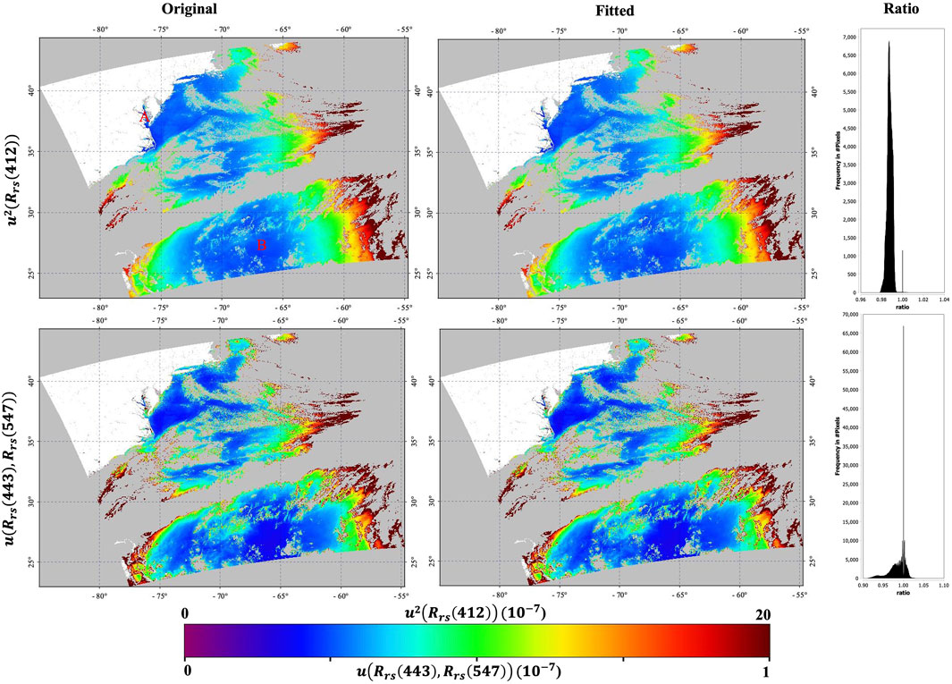
Figure 1. u²(R_rs(412)) and u(R_rs(443), R_rs(547)) from the derivative approach (denoted by “original”) compared with that calculated from the third-degree polynomial fitting (denoted by “fitted”). The ratio is obtained by dividing the fitted value by the original value. MODIS data acquired on 28 January 2012 are used here. Pixels denoted by A and B are used to show the polynomial fitting. The white region is land, and the gray color means no data.

Figure 2

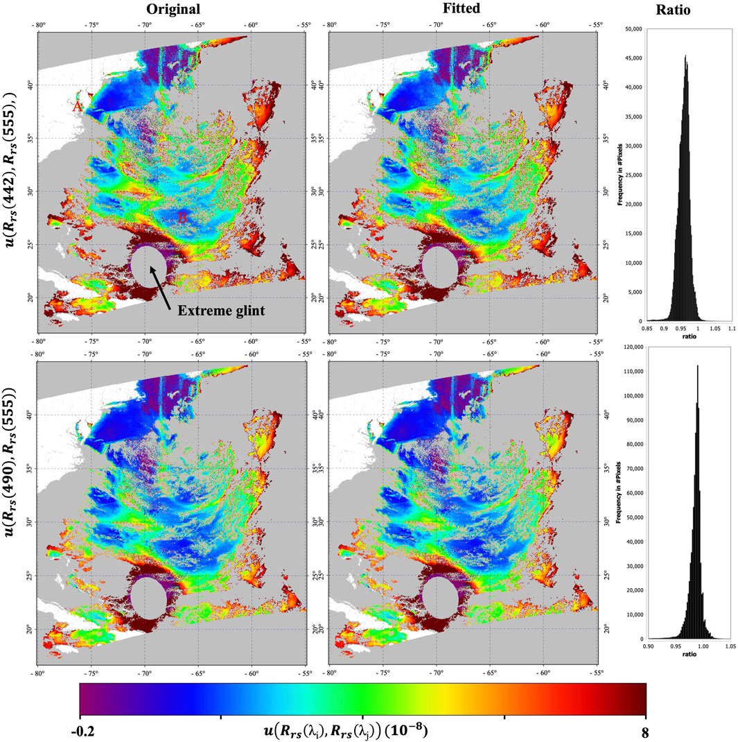
Figure 2. As Figure 1 but for the fitting of u(R_rs(442), R_rs(490)) and u(R_rs(442), R_rs(555)) of OCI data on 13 May 2024. Pixels denoted by A and B are used to show the polynomial fitting. Extreme glint means that the glint coefficient is higher than 0.03.

Figure 3 further shows the comparison between u(R_rs(λ_j), R_rs(λ_i)) calculated from the derivative approach and that derived from third-degree polynomial fitting at the global scale. u(R_rs(λ_j), R_rs(λ_i)) is relatively higher in coastal and high-latitude regions. Like Figure 2, the third-degree polynomial fitted u(R_rs(λ_j), R_rs(λ_i)) matches very well with the original one, showing a similar spatial pattern, with mean ratios (standard deviations) of 0.989 (0.002), 0.99 (0.015), and 0.83(1.866) for u(R_rs(412)), u(R_rs(443), R_rs(547)), and u(R_rs(443), R_rs(667)), respectively. While the distribution is broader for u(R_rs(443), R_rs(667)), the absolute values are small, so this is a ratio of very small numbers.

Figure 3

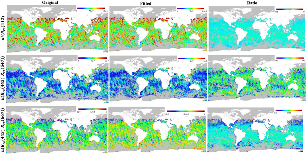
Figure 3. As Figure 1, but at a global scale using MODIS data during 3–10 December 2019.

While Figures 1–3 show that fitted u(R_rs(λ_j), R_rs(λ_i)) has a similar spatial pattern as the original fully computed one, Figure 4 shows a time series u(R_rs(λ_j), R_rs(λ_i)) derived from the fitting compared with the original over MOBY during 2002–2010, which shows consistent temporal variations, although u(R_rs(443), R_rs(667)) exhibits some bias. Considering the small value, such bias should not affect the uncertainty in the downstream products too much.

Figure 4

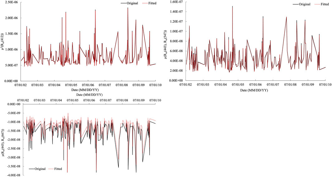
Figure 4. u(R_rs(λ_j), R_rs(λ_i)) derived from the polynomial fitting compared with that derived from the derivative approach based on MODIS data over MOBY during 2002–2010.

4.2 Fitting of u(R_rs(λ_i), R_rs(λ)) as a function of wavelength

Figure 5 shows two examples of the fitting of u(R_rs(412), R_rs(λ)) and u(R_rs(531), R_rs(λ)) versus wavelength over two pixels (denoted by A and B in Figure 1, with pixel A over coastal waters near the Chesapeake Bay and pixel B over open ocean waters of the North Atlantic Ocean. Like Figures 5, 6 shows examples of the fitting of u(R_rs(413), R_rs(λ)) and u(R_rs(530), R_rs(λ)) for OCI over two pixels (denoted by A and B in Figure 2). The high R-squared value (>0.99) indicates the reliability of the fitting. Note the comparatively higher error covariance over coastal waters than over clear waters across visible wavelengths.

Figure 5

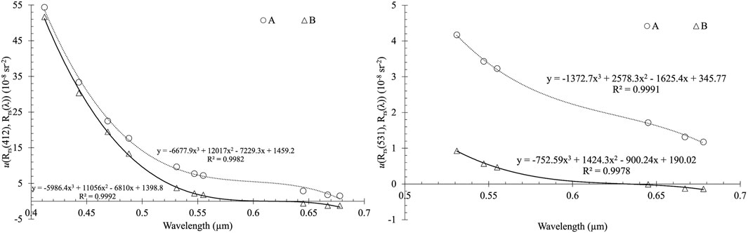
Figure 5. Third-degree polynomial fitting of (A) u(R_rs(412), R_rs(λ)) and (B) u(R_rs(531), R_rs(λ)) versus wavelength over two pixels denoted by A and B in Figure 1. R² is the R-squared value for the fitting.

Figure 6

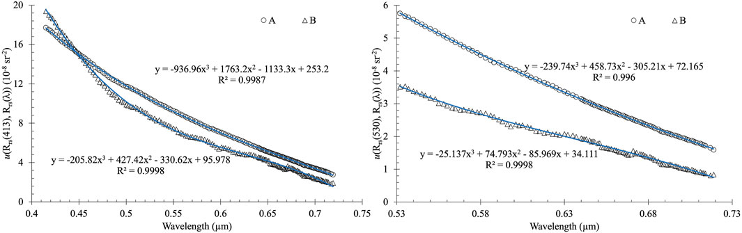
Figure 6. As Figure 5, but for OCI data over two pixels denoted by A (coastal) and B (open ocean) in Figure 2.

4.3 Effect on uncertainty in chl_a and K_d(490)

R_rs(λ) is fundamental to deriving a host of bio-optical and biogeochemical properties of the water column. Taking chl_a and K_d(490) as examples, the effect of using the polynomial approximation for error covariance in R_rs(λ) is evaluated on u²(chl_a) and u²(K_d(490)). Specifically, u²(chl_a) and u²(K_d(490)) calculated using u(R_rs(λ_j), R_rs(λ_i)) derived from the derivative approach are compared with those calculated using u(R_rs(λ_j), R_rs(λ_i)) derived from polynomial fitting. We can see from Figure 7 that the relative uncertainty in chl_a and K_d(490), denoted by δ(chl_a) (u(chl_a) × 100/chl_a) and δ(K_d(490)) (u(K_d(490)) × 100/K_d(490)), calculated using original and polynomial fitted error covariance show similar spatial variation, with the absolute difference smaller than 0.5%.

Figure 7

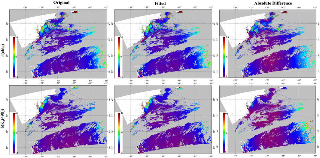
Figure 7. δ(chl_a) and δ(K_d(490)) calculated using the original and the polynomial fitted error covariance in R_rs(λ) retrieved from MODIS data shown in Figure 1. The absolute difference is between δ(chl_a) and δ(K_d(490)) calculated in those two ways.

5 Conclusion

We assessed how well a polynomial fitting can reproduce the full spectral error covariance in R_rs from MODIS and OCI data, with the goal of decreasing the Level-2 file size and therefore facilitating efficient delivery of those products. We found that a third-degree polynomial works well for data processed using the MSEPS algorithm, which is the standard algorithm used in R_rs retrieval for all global multispectral ocean color missions processed by NASA. We first evaluated the fitting by comparing the values numerically to the original error covariance source data, finding ratio close to 1 (typically from 0.95 to 1.05). We also found that using the fitted approximation of the covariance matrix to estimate the uncertainty of the downstream products chl_a and K_d(490) led to only a small absolute difference of the relative uncertainty that was less than 0.5%. Thus, we conclude that the accuracy of the approximation appears sufficient for most data user purposes.

By including the coefficients derived from polynomial fitting rather than the full ∑R_rs, a standard Level-2 file will decrease from ∼231 MB to ∼165 MB for a 5-min granule shown in Figure 1. The standard Level-2 file contains τ_a (869), Ångström exponent, R_rs(λ) at wavelengths from 412–678 nm, chl_a, K_d(490), particulate inorganic carbon (pic), particulate organic carbon (poc), instantaneous photosynthetically available radiation (ipar), normalized fluorescence line height (nflh), and photosynthetically available radiation (par). Taking the OCI 5-min granule in Figure 2 as an example, the Level-2 file would be ∼60 GB, including full ∑R_rs, which decreases to ∼1.7 GB by including the polynomial fitting coefficients.

Another benefit of using the polynomial model to estimate R_rs(λ) error covariance terms comes into play during operational data processing. As highlighted in this study, the full set of sensor bands is not always used in bio-optical algorithms (e.g., two for K_d(490) and four for chl_a). The approach described can thus facilitate dynamic computation of only the ∑R_rs terms required by an algorithm, thereby reducing system memory overheads and improving computational efficiency.

Data availability statement

The raw data supporting the conclusions of this article will be made available by the authors, without undue reservation.

Author contributions

MZ: Conceptualization, Data curation, Investigation, Validation, Writing – original draft, Writing – review and editing. AI: Writing – review and editing. BF: Conceptualization, Funding acquisition, Supervision, Writing – review and editing. AS: Writing – review and editing. PW: Funding acquisition, Writing – review and editing. LM: Writing – review and editing.

Funding

The author(s) declare that financial support was received for the research and/or publication of this article. NASA Terra and Aqua Senior Review for MODIS algorithm maintenance and the NASA PACE Project.

Acknowledgments

We are grateful to NASA’s Ocean Biology Distributed Active Archive Center for making available all the in situ data and MODIS, OCI data used in our analysis.

Conflict of interest

Author MZ was employed by Science Application International Corp. Author LM was employed by Go2Q Pty Ltd.

The remaining authors declare that the research was conducted in the absence of any commercial or financial relationships that could be construed as a potential conflict of interest.

Generative AI statement

The author(s) declare that no Generative AI was used in the creation of this manuscript.

Any alternative text (alt text) provided alongside figures in this article has been generated by Frontiers with the support of artificial intelligence and reasonable efforts have been made to ensure accuracy, including review by the authors wherever possible. If you identify any issues, please contact us.

Publisher’s note

All claims expressed in this article are solely those of the authors and do not necessarily represent those of their affiliated organizations, or those of the publisher, the editors and the reviewers. Any product that may be evaluated in this article, or claim that may be made by its manufacturer, is not guaranteed or endorsed by the publisher.

References

Ahmad, Z., and Franz, B. A. (2015). Ocean color retrieval using multiple-scattering epsilon values. Int. Ocean Color Sci. Meet.

Google Scholar

Cael, B. B., Bisson, K., Boss, E., Dutkiewicz, S., and Henson, S. (2023). Global climate-change trends detected in indicators of ocean ecology. Nature 619, 551–554. doi:10.1038/s41586-023-06321-z

PubMed Abstract | CrossRef Full Text | Google Scholar

Clark, D., Murphy, M., Yarbrough, M., Feinholz, M., Flora, S., Broenkow, W., et al. (2003). MOBY, A radiometric buoy for performance monitoring and vicarious calibration of satellite ocean color sensors: measurement and data analysis protocols. SeaWiFs Postlaunch Tech. Rep. Ser. Available online at: https://www.nist.gov/publications/moby-radiometric-buoy-performance-monitoring-and-vicarious-calibration-satellite-ocean (Accessed December 5, 2024).

Google Scholar

Coddington, O. M., Richard, E. C., Harber, D., Pilewskie, P., Woods, T. N., Chance, K., et al. (2021). The TSIS-1 hybrid solar reference spectrum. Geophys. Res. Lett. 48, e2020GL091709. doi:10.1029/2020GL091709

PubMed Abstract | CrossRef Full Text | Google Scholar

Cox, C., and Munk, W. (1954). Measurement of the roughness of the Sea surface from photographs of the Sun?s glitter. J. Opt. Soc. Am. 44, 838–850. doi:10.1364/JOSA.44.000838

CrossRef Full Text | Google Scholar

Dutkiewicz, S., Hickman, A. E., Jahn, O., Henson, S., Beaulieu, C., and Monier, E. (2019). Ocean colour signature of climate change. Nat. Commun. 10, 578. doi:10.1038/s41467-019-08457-x

PubMed Abstract | CrossRef Full Text | Google Scholar

Fox, N. (2010). A guide to expression of uncertainty of measurements. GEO. Available online at: https://qa4eo.org/docs/QA4EO-QAEO-GEN-DQK-006_v4.0.pdf (Accessed September 10, 2025).

Google Scholar

Hu, C., Feng, L., Lee, Z., Franz, B. A., Bailey, S. W., Werdell, P. J., et al. (2019). Improving satellite global chlorophyll a data products through Algorithm Refinement and data recovery. J. Geophys. Res. Oceans 124, 1524–1543. doi:10.1029/2019JC014941

CrossRef Full Text | Google Scholar

IOCCG (2019). “Uncertainties in Ocean colour remote sensing,” in International Ocean Colour Coordinating Group. Dartmouth, Canada. Available online at: https://ioccg.org/wp-content/uploads/2020/01/ioccg-report-18-uncertainties-rr.pdf (Accessed September 10, 2025).

Google Scholar

Jackson, T., Sathyendranath, S., and Mélin, F. (2017). An improved optical classification scheme for the Ocean Colour Essential climate Variable and its applications. Remote Sens. Environ. 203, 152–161. doi:10.1016/j.rse.2017.03.036

CrossRef Full Text | Google Scholar

JCGM (2011). Evaluation of measurementdata — supplement 2 to the “expression of uncertainty in measurement” -Extension to any number of output quantities.

Google Scholar

Lamquin, N., Mangin, A., Mazeran, C., Bourg, B., Bruniquel, V., and D’Andon, O. F. (2013). Pixel-by-pixel uncertainty propagation in OLCI clear water branch. Available online at: https://user.eumetsat.int/s3/eup-strapi-media/pdf_s3_atbd_olci_l2_un_e9ee7d9041.pdf (Accessed September 11, 2025).

Google Scholar

McKinna, L. I. W., Cetinić, I., Chase, A. P., and Werdell, P. J. (2019). Approach for propagating radiometric data uncertainties through NASA Ocean color algorithms. Front. Earth Sci. 7, 176. doi:10.3389/feart.2019.00176

PubMed Abstract | CrossRef Full Text | Google Scholar

Morel, A., Antoine, D., and Gentili, B. (2002). Bidirectional reflectance of oceanic waters: accounting for Raman emission and varying particle scattering phase function. Appl. Opt. 41, 6289–6306. doi:10.1364/AO.41.006289

PubMed Abstract | CrossRef Full Text | Google Scholar

NASA (2023). Diffuse attenuation coefficient for downwelling irradiance at 490 nm (Kd). Available online at: https://oceancolor.gsfc.nasa.gov/resources/atbd/kd/.

Google Scholar

O’Reilly, J. E., and Werdell, P. J. (2019). Chlorophyll algorithms for ocean color sensors - OC4, OC5 and OC6. Remote Sens. Environ. 229, 32–47. doi:10.1016/j.rse.2019.04.021

PubMed Abstract | CrossRef Full Text | Google Scholar

Stramska, M., and Petelski, T. (2003). Observations of oceanic whitecaps in the north polar waters of the Atlantic. J. Geophys. Res. Oceans 108, 2002JC001321–a. doi:10.1029/2002JC001321

CrossRef Full Text | Google Scholar

Thuillier, G., Floyd, L., Woods, T. N., Cebula, R., Hilsenrath, E., Hersé, M., et al. (2004). Solar irradiance reference spectra for two solar active levels. Adv. Space Res. 34, 256–261. doi:10.1016/j.asr.2002.12.004

CrossRef Full Text | Google Scholar

Wang, M., and Bailey, S. W. (2001). Correction of sun glint contamination on the SeaWiFS ocean and atmosphere products. Appl. Opt. 40, 4790–4798. doi:10.1364/AO.40.004790

PubMed Abstract | CrossRef Full Text | Google Scholar

Zhang, M., Ibrahim, A., Franz, B. A., Ahmad, Z., and Sayer, A. M. (2022). Estimating pixel-level uncertainty in ocean color retrievals from MODIS. Opt. Express 30, 31415–31438. doi:10.1364/OE.460735

PubMed Abstract | CrossRef Full Text | Google Scholar

Zhang, M., Ibrahim, A., Franz, B. A., Sayer, A. M., Werdell, P. J., and McKinna, L. I. (2024). Spectral correlation in MODIS water-leaving reflectance retrieval uncertainty. Opt. Express 32, 2490–2506. doi:10.1364/OE.502561

PubMed Abstract | CrossRef Full Text | Google Scholar