3D colored point cloud classification of a deep-sea cold-water coral and sponge habitat using geometric features and machine learning algorithms

Classification of benthic habitats in the deep sea is instrumental in managing and monitoring marine ecosystems as it provides distinct units for which changes can be quantified over time. These applications require automatic classification approaches with reasonable accuracy to ensure efficiency and robustness. The use of 3D point clouds is currently emerging in deep-sea benthic classification as it allows for high-resolution representation of the 3D structure (i.e., geometry), texture, and composition of complex benthic habitats such as those created by structure-forming cold-water corals. Point clouds were derived from remotely operated vehicle video surveys of three vertical walls (depth range 1400–1900 m) along the Charlie-Gibbs Fracture Zone, North Atlantic. In addition to RGB values, this research incorporated nine geometric features derived from structure-from-motion 3D point clouds to classify coral and sponge colonies. Three unsupervised (k-means (KM), fuzzy c-means (FCM), and Gaussian mixture model (GMM)) and three supervised (decision tree (DT), random forest (RF), and linear discriminant analysis (LDA)) machine learning (ML) algorithms were compared and assessed for accuracy and reliability. The ML classifiers were used to build full-coverage seafloor predictions for three classes, namely, seabed, sponges, and corals. The KM, GMM, and FCM achieved an average overall accuracy of 74.87%, 71.94%, and 70.77%, respectively, while the RF, LDA, and DT achieved 84.50%, 84.01%, and 79.90%, respectively. Overall, the supervised ML classifiers outperformed the unsupervised ML classifiers. In particular, the RF classifier demonstrated the highest overall classification accuracy and F1-score for individual classes, with an average of 89.09%, 67.12%, and 41.60% for the seabed, sponges, and corals, respectively. In addition, the spatial coherence of the point clouds was considered and improved the results’ overall accuracy and F1-score by up to 9% and 12%, respectively. Results showed that incorporating geometric features, traditionally employed in terrestrial and shallow-water LiDAR surveys, in combination with RGB values is suitable for high-resolution deep-sea benthic 3D point clouds classification.

1 Introduction

Seafloor classification has gained the interest of scientists for its importance in supporting activities such as resource management, ecological protection, and monitoring of environmental change (Brown et al., 2012). With the significant changes currently predicted to our oceans, many species are expected to be affected (Talukder et al., 2022). Cold-water corals and sponges are important components of marine benthic ecosystems, as they play critical roles in maintaining high levels of biodiversity (Henry and Roberts, 2017), as well as in carbon cycling and sequestration (Cathalot et al., 2015; Soetaert et al., 2016; Titschack et al., 2016). Moreover, they provide habitat for a range of other organisms, increasing habitat complexity and biodiversity (Henry and Roberts, 2017), yet they are predicted to undergo a significant decrease in extent in the North Atlantic (Morato et al., 2020). This is due to climate change, including ocean acidification, rising temperature, and food supply change (Morato et al., 2020), as well as anthropogenic activities such as bottom trawling, oil exploration and production, and submarine cables (Ragnarsson et al., 2017). Monitoring these habitats at high resolution and in three dimensions (3D) to quantify habitat change is needed, but particularly challenging in the deep sea.

High resolution seafloor classification in coastal zones and shallow waters (i.e., water depth ranges from 1 to 30 m) can be achieved from airborne LiDAR bathymetry data (Zavalas et al., 2014; Parrish et al., 2016; Letard et al., 2021). Many studies have converted the 3D LiDAR point clouds into 2D raster images and then applied classification techniques, similarly to underwater mapping from bathymetric data (Zavalas et al., 2014; Parrish et al., 2016; Letard et al., 2021). However, these studies lose the advantage of considering the 3D geometry of underwater habitats in the classification process. 3D point clouds can provide additional spatial information, especially for complex habitats such as cold-water coral reefs and sponge gardens, producing the more detailed and accurate representations needed for robust monitoring.

Unfortunately, bathymetric LiDAR is not widely available for deep-water habitats, and alternate approaches need to be considered to obtain 3D point clouds. Underwater videos recorded using high-definition (HD) cameras mounted on remotely operated vehicles (ROVs) are valuable remote sensing tools for monitoring changes and distribution of benthic habitats with high spatial and temporal resolution (Piazza et al., 2019; Price et al., 2019; McGeady et al., 2023). These videos can, in turn, be converted from 2D images to 3D point clouds using photogrammetric reconstruction methods such as structure-from-motion (SfM) (Robert et al., 2017; Pierce et al., 2021; De Oliveira et al., 2021; Ventura et al., 2023). SfM is a photogrammetric technique utilized for generating 3D models from sequences of overlapping 2D images, which can deal with sets of unordered and heterogeneous images without prior knowledge of the camera parameters (Westoby et al., 2012). Similar to bathymetric LiDAR, geometric features (e.g., linearity, planarity, scattering) based on eigenvalues and eigenvectors of neighborhood points can be derived (Weinmann et al., 2015; Hackel et al., 2016; Thomas et al., 2018; Morsy and Shaker, 2022), but one advantage over LiDAR is that RGB (Red, Green, and Blue) values of points are also available.

Several attempts have been carried out to automate the classification process of underwater images, with recent advances in computer vision suggesting various ML algorithms for benthic classification (e.g., Pierce et al., 2021; Mohamed et al., 2022; Ternon et al., 2022) and 3D point cloud classification for shallow-water applications (e.g., Parrish et al., 2016; Pierce et al., 2021; Letard et al., 2022). ML classifiers can be categorized into unsupervised or supervised. Unsupervised ML classifiers first cluster points based on spectral and/or geometric properties using algorithms, such as k-means, and fuzzy c-means, among others (Lucieer and Lamarche, 2011; Mohamed et al., 2022). The obtained clusters are then assigned to predefined classes. Unsupervised ML classifiers do not require prior knowledge of the area of interest, as no training samples are used. In addition, the analyst has only control over selecting the number of clusters, number of iterations, and convergence thresholds. Unsupervised methods may result in unrepresentative classes and are time-consuming to interpret and assign clusters to their associated classes (Mather and Tso, 2016). On the other hand, supervised ML classifiers (e.g., decision tree, support vector machines, and random forests, among others) create models that have learned based on a representative training dataset and are therefore able to generalize unseen data (Mahmood et al., 2018; Mahmood et al., 2020; De Oliveira et al., 2021). However, in order to derive ecologically meaningful information, manual annotations of a large number of underwater images are required, a process which is tedious, error-prone, and time-consuming (Mahmood et al., 2020; Mather and Tso, 2016). For instance, 10–30 min can be required for a marine expert to produce fully annotated pixel-level labels for a single image (Mahmood et al., 2018). Currently, manual annotations are required for result assessment of both supervised and unsupervised ML classifiers, and remains a major bottleneck for benthic studies using imagery, highlighting the pressing need to automate this process (Yuval et al., 2021).

The application of ML classifiers for deep-sea benthic classification has not been explored extensively. However, De Oliveira et al. (2021), De Oliveira et al. (2022) evaluated several 3D point-based ML classification methods for cold-water coral reefs identification, while Price et al. (2021) classified 3D point clouds of deep-sea habitats into corals and non-corals. In this research, we consider three unsupervised and three supervised ML classifiers for deep-sea benthic classification of corals and sponges. The ML classifiers incorporate geometric features along with RGB values and are evaluated against expert manual annotations for multi-class benthic classification of deep-sea vertical cliffs inhabited by cold-water coral and sponges.

2 Materials and methods

2.1 Study area and data acquisition

The Charlie-Gibbs Fracture Zone (CGFZ), located at 53° 15′49″N and 35° 31′12″W (Figure 1), consists of two parallel fractures which offset the Mid-Atlantic Ridge by about 370 km. The highly variable seafloor bathymetry (700–4,500 m) causes a heterogeneous environment characterized by nutrient-rich water mass exchanges, creating diverse and biologically productive deep-sea ecosystems (Calvert and Whitmarsh, 1986; Alt et al., 2019; Skolotnev et al., 2021). This makes the CGFZ a recognized highly biodiverse area of ecological importance (Mortensen et al., 2008). Hence, the CGFZ’s seafloor and water column in the south (OSPAR, 2010) and the water column in the north were declared High Seas Marine Protected Areas (OSPAR, 2012). However, the presence of ecosystem engineers, such as cold-water corals and sponges, in the northern area highlights the need for detailed surveys and high-resolution mapping to help support decisions on its protection status (Keogh et al., 2022).

Figure 1

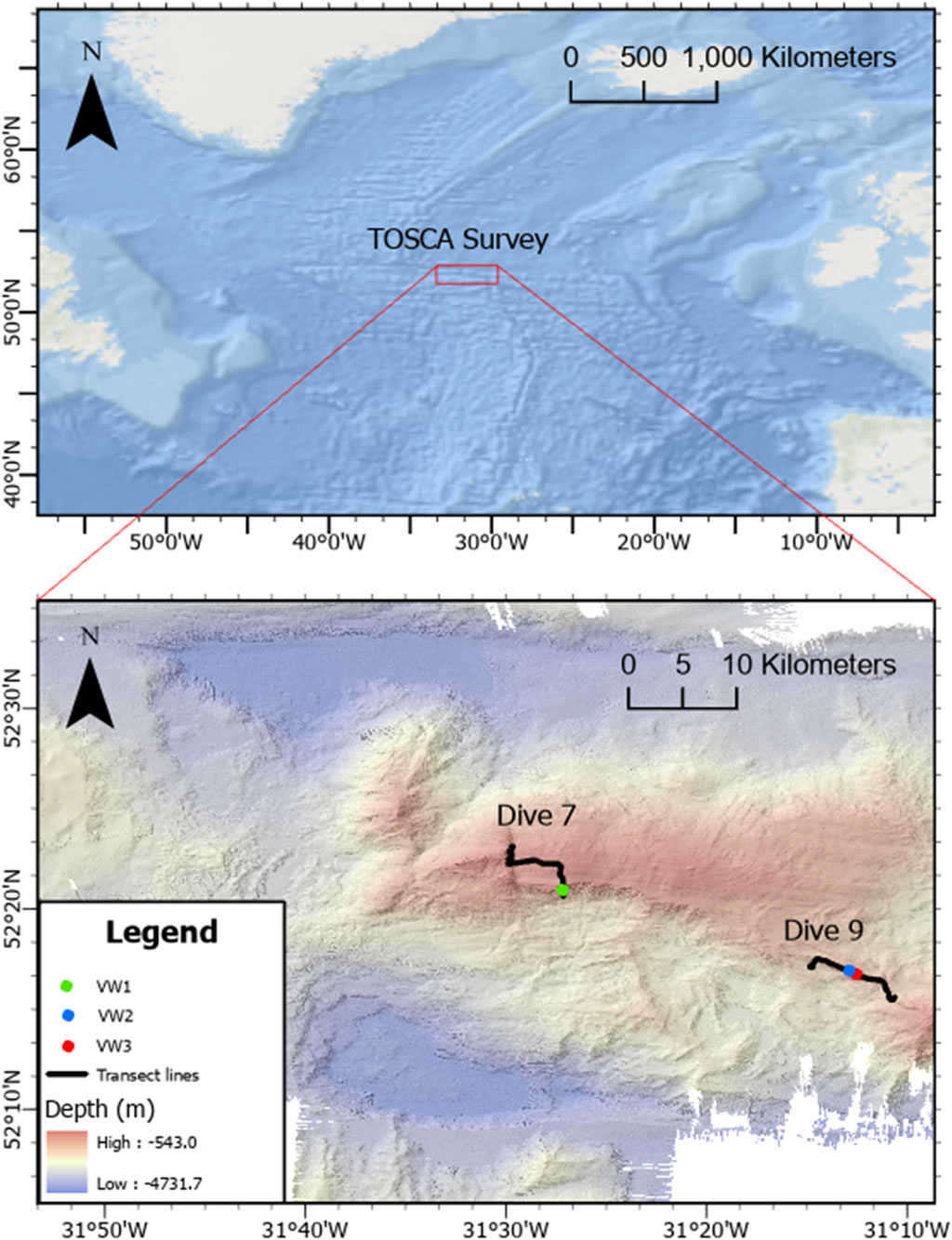
Figure 1. Upper: Location of the Charlie-Gibbs Fracture Zone (CGFZ) with the Tectonic Ocean Spreading at the Charlie-Gibbs Fracture Zone (TOSCA) survey marked by a red box. Bathymetry background is a World Ocean Basemap obtained from ArcGIS Pro. Lower: Detailed bathymetry of the TOSCA survey, transect locations of Dive 7 and Dive 9, and locations of vertical walls (VWs) along survey tracks.

In summer 2018, the CGFZ was surveyed during the Tectonic Ocean Spreading of the Charlie-Gibbs Fracture Zone’s (TOSCA) expedition onboard the research vessel Celtic Explorer (CE18008) (Figure 1). A HD oblique-facing camera, Kongsberg Maritime OE14-502a HDTV, was mounted on the ROV Holland I to video record (1080i resolution at 25 frames per second) benthic habitats. The position of the ROV was continuously recorded using Ultra Short Baseline (USBL) systems (IXSEA GAPS USBL and Sonardyne Ranger 2 USBL). One image per second extracted from the video sections of two dives: Dive 7 and Dive 9, (Figure 1), were used to produce dense point clouds of three vertical walls (VWs): VW1 from Dive 7; VW2 and VW3 from Dive 9. Dive 7 exhibited a high density of Scleractinian corals, while Dive 9 exhibited a high abundance of Demospongiae and Hexactinellid sponges. Both vertical walls also exhibited a scatter of corals order Scleralcyonacea.

2.2 Methodology

The seafloor classification workflow, Figure 2, started with 3D point cloud reconstruction from underwater images using the SfM technique, followed by manual annotation into three classes: seabed, sponges, and corals (details provided in Section 3.1). Nine geometric features were subsequently derived from the 3D point clouds and utilized as input for the ML classifiers (three unsupervised and three supervised ML algorithms) in addition to the RGB values of the point clouds. The unsupervised ML algorithms were k-means (KM), fuzzy c-means (FCM), and Gaussian mixture model (GMM), while the supervised ML algorithms were decision tree (DT), random forest (RF), and quadratic discriminant analysis (QDA). As both, the unsupervised and supervised ML classifiers employed are point-based classification methods, which can suffer from salt and pepper artefacts (Liang et al., 2021), the spatial coherence of the point clouds was considered to improve classification accuracy. The six classifiers were then evaluated in terms of overall accuracy as well as recall, precision, and F1-score for individual classes.

Figure 2

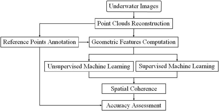
Figure 2. Seafloor classification workflow.

2.2.1 Point clouds reconstruction and reference points annotation

Underwater images were extracted from the HD videos as a frame per second using Blender software (version 2.92) (Blender Foundation, 2021). The coordinates of each frame were obtained from the USBL data and exported as CSV files. The images and coordinates files were then imported to Agisoft Metashape software (version 1.6.1) (Agisoft, 2020), where the coordinates of the images were projected to UTM zone 25N. The 3D point clouds were reconstructed by applying the following steps in Agisoft Metashape software: 1) creating a sparse point cloud, 2) masking of ROV parts from images, 3) scaling the reconstruction based on two lasers separated by 10 cm, 4) optimizing camera alignment 5) creating a dense point cloud, 6) cleaning, and 7) exporting the dense point clouds as XYZ files (more details on the reconstructions are available in Yánez-Suárez et al. (2025)). Figure 3 shows the 3D point clouds of the three vertical walls, and their specifications are provided in Table 1. Corals and sponges (>4 cm) were manually annotated within the dense point clouds using the free-form selection tool in Agisoft Metashape software and assigned classes (Marcillat et al., 2024). Approximately 7% (600,192 points), 15% (2,648,414 points), and 10% (1,066,139 points) of the total number of points of VW1, VW2, and VW3, respectively were labeled as reference data (i.e., ground truth), with the seabed class accounting for 51%–72% of the annotations (Table 1).

Figure 3

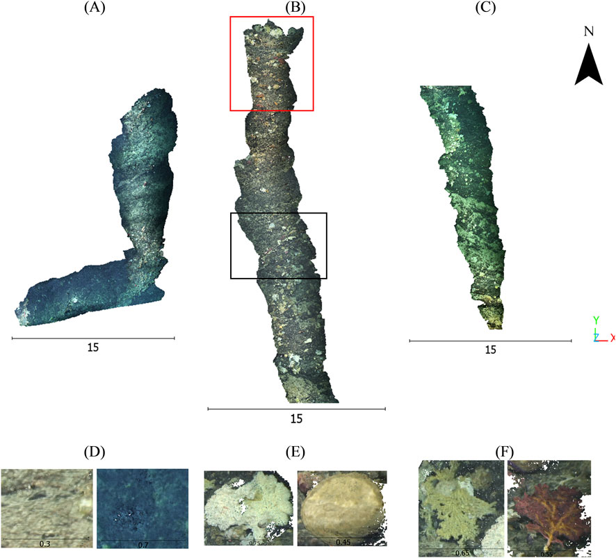
Figure 3. 3D point cloud reconstructions of (A) vertical wall 1 (VW1), (B) vertical wall 2 (VW2), and (C) vertical wall 3 (VW3); with examples of the three classes annotated: (D) seabed, (E) sponges, and (F) corals. Scale is in meter. A portion of the data in the red box is displayed in Figures 4, 6, while the black box is displayed in Figure 5.

Table 1

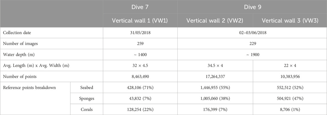
Table 1. Dataset specifications.

2.2.2 Geometric features computation

Nine geometric features were derived from SfM-generated point clouds. The features included eight eigenvalues-based features (Weinmann et al., 2015), namely, linearity (L), planarity (P), Sphericity or Scattering (S), omni-variance (O), anisotropy (A), Eigen entropy (E), surface variation (SV), and sum (∑), in addition to verticality (V) (Demantké et al., 2012) (Table 2). These features rely on surrounding neighborhood points, and a neighborhood selection method must be specified. Previously, studies have investigated three standard neighborhood selection methods, namely, K-nearest neighbor, spherical, and cylindrical (Weinmann et al., 2014; Thomas et al., 2018; Mohamed et al., 2021). In this research, the spherical neighborhood method was applied as it is suitable for a dataset with uniform point density. Thus, for query point x, all neighbor points within a sphere with a predefined radius r were considered. After testing various values, a 5 cm radius was chosen to maintain a balance between including sufficient neighboring points for statistical robustness and avoiding outliers that could skew the results. This choice ensured that the analysis effectively captured relevant geometric features without introducing excessive noise from distant points. A covariance matrix (Cov) was then derived as defined in Equation 1 (Jutzi and Gross, 2009). The eigenvalues (λ₁, λ₂, λ₃) and eigenvectors (ν₁, ν₂, ν₃) were then calculated and used for geometric features computation.

$\text{Cov}=\frac{1}{N}{\displaystyle \sum _{i=1}^N}\left(x_i-\overline{x}\right){\left(x_i-\overline{x}\right)}^T(1)$

where:

Table 2

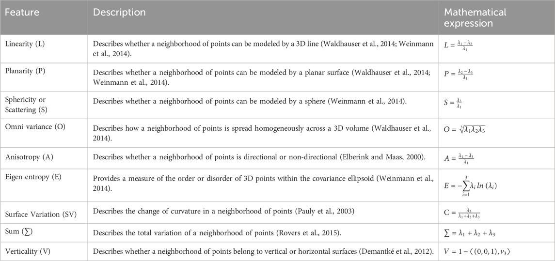
Table 2. Geometric features description. λ₁, λ₂ and λ₃ are the eigenvalues, and ν₃ is the third eigenvector.

N = number of points within the neighborhood

x_i = coordinates array of point i.

$\overline{x}$ = mean coordinates array

The point clouds of the three vertical walls were imported to the CloudCompare software (v2.12.0) (CloudCompare, 2022), and the nine geometric features were computed based on a spherical neighborhood (5 cm radius) (Figure 4). Combined with each point’s RGB values, twelve features (R, G, B, L, P, S, O, A, E, SV, Σ, and V) were subsequently used in the classification process.

Figure 4

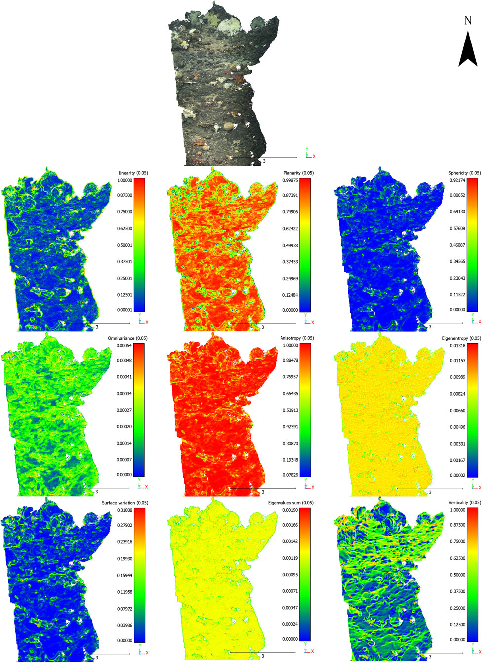
Figure 4. A portion of the original point cloud from vertical wall 2 (VW2) with all geometric features. Feature descriptions are provided in Table 2. Geometric features were computed from neighbor points within a sphere of 0.05 m radius. Scale is in meter.

2.2.3 Training and testing datasets

The annotated data were divided into two parts: training and testing. The training part was used to train a supervised model, and the model was then evaluated with the testing portion of the dataset. Previous studies have randomly selected ML classifiers’ training/testing datasets (Zavalas et al., 2014; Mohamed et al., 2018; Mohamed et al., 2020; Letard et al., 2021). However, this introduced bias because of the high spatial correlation between training and testing datasets. Therefore, in this research, the annotated data were divided into four spatially continuous parts, each of which was used in turn as the testing dataset (25%), while the remaining parts were used as the training dataset (75%). In addition, all training points within a sphere of a 5 cm radius around the testing points were removed to limit the effect of spatial autocorrelation (Letard et al., 2022). The data division, point cloud classification using unsupervised and supervised ML, and accuracy assessment were implemented using the Python programming language, mainly utilizing the scikit-learn library (Pedregosa et al., 2011).

2.2.4 Unsupervised ML algorithms

As aforementioned, three unsupervised algorithms were applied in this research. KM works by partitioning a dataset into a set number of clusters, k, predefined by the analyst (MacQueen, 1967). FCM is a soft clustering algorithm where each data point is assigned a likelihood or probability score of belonging to that cluster (Bezdek et al., 1984). GMM is a probabilistic clustering algorithm that separates the data points into a finite number of Gaussian distributions (i.e., components) (Maugis et al., 2009). GMM, unlike KM, considers the variances of clusters. In addition, it is a soft clustering algorithm since it provides the probability that a given data point belongs to each possible cluster (He et al., 2010). The three algorithms are described in detail in the Supplementary Section 1.

Scaling of the input features is always required as a preprocessing step for unsupervised ML algorithms (Coates and Ng, 2012). This is essential when comparing measurements with different units because features measured at different scales do not contribute equally to the analysis and might create a bias. Therefore, the twelve features were first standardized by removing the mean (i.e., mean = 0) and scaled to unit variance (i.e., standard deviation = 1). As, the output clusters of the unsupervised ML do not always correspond to informational classes, one or more clusters were manually assigned to one of the predefined classes (e.g., seabed, sponges, or corals) based on three criteria: 1) the visual interpretation of the results, 2) the highest OA, and 3) the number of points of each class was proportional to the reference data. We estimated the optimal number of clusters (k = 6) using the elbow method (Marutho et al., 2018).

2.2.5 Supervised ML algorithms

Three supervised algorithms, based on different principles, were employed in this research. DT is a rule-based learning that conducts a series of hierarchically organized nodes and branches (Quinlan, 1986). RF is an ensemble algorithm consisting of multiple decision trees, in which each decision tree provides a vote to assign each class to an input point (Breiman, 2001). Ultimately, each point is assigned to the most frequent class among all trees. LDA is a statistical model that fits a Gaussian density function to each class and detects a linear boundary between them (Ye and Yu, 2005). It is easily computed and has no hyperparameters to tune. The three algorithms are described in detail in the Supplementary Section 2.

The first step in supervised ML classification was to define different parameters for each classifier. For DT and RF parameters settings, the function to measure the quality of a split was set to “Gini impurity,” and the class weight was set to “balanced” to consider the percentage of classes in the training dataset while creating the model. The “balanced” mode adjusts the importance (weights) of different classes based on their frequency in the training dataset. This adjustment is crucial in scenarios where some classes have significantly more samples than others (class imbalance). The weights are determined in such a way that classes with fewer samples receive higher weights, while classes with many samples receive lower weights. This helps the model pay more attention to underrepresented classes during training. For hyperparameters estimation, a grid search was conducted to estimate the number of features to be used in splitting a node and the maximum depth of the tree for both the DT and RF classifiers, in addition to the number of trees in the forest for the RF classifier. As a result of the grid search, the number of features was set to the square root “sqrt” of the input features. The maximum depth of the tree was set to “None,” meaning that the nodes were expanded until all leaves were pure or until all leaves contained less than the minimum split samples (i.e., 2). The number of trees in RF was set to 300. On the other hand, the parameters of the LDA classifier were set to the default settings.

2.2.6 Spatial coherence

Generally, point-based classification methods produced noisy results, known as salt and pepper artefacts (Liang et al., 2021). This is attributed to the fact that they do not consider the spatial coherence of points’ neighborhoods. Each point was classified according to its RGB values and position in the feature space. Thus, the probability of a data point belonging to a particular class was affected significantly by its neighbors. Therefore, spatial coherence was considered by applying a max voting 3D filter. This filter assigned each point to the class that occurred most frequently in its neighborhood within a sphere of 2 cm radius. This value was specified because any object with a dimension less than 4 cm was not labeled during reference data annotation.

2.2.7 Accuracy assessment

The accuracy assessment for benthic habitat classification was conducted using the retained portion of the annotated reference data (i.e., the testing dataset). The confusion matrix was constructed, and accuracy metrics were computed, including overall accuracy (OA), precision, recall, and F1-score as given in Equations 2–5, respectively.

$OA=\frac{TP+TN}{TP+TN+FP+FN}(2)$

$Precision=\frac{TP}{TP+FP}(3)$

$Recall=\frac{TP}{TP+FN}(4)$

$F1-score=\frac{2*Precision*Recall}{Precision+Recall}(5)$

Where true positive (TP), false positive (FP), true negative (TN), and false negative (FN) represent the number of points of correctly identified class, incorrectly identified class, correctly rejected class, and incorrectly rejected class, respectively. The OA denotes the ratio of correctly predicted data to the total observations (Congalton, 1991), precision refers to the ratio of correctly predicted positive data to the total predicted positive data, recall refers to the ratio of correctly predicted positive data to all observations in the actual class, and F1-Score is the weighted average of precision and recall (Goutte and Gaussier, 2005).

3 Results

3.1 Unsupervised ML classification

For the unsupervised ML classifiers (KM, FCM, or GMM), six clusters were identified as optimal (see Supplementary Figure S1), and assigned to the three classes. The KM classifier demonstrated the highest average OA across all walls with 74.87%, followed by GMM with 71.94%, and then FCM with 70.77% (Table 3; Supplementary Table S1). Regarding the individual classes, KM obtained the highest average F1-score, 83.08% and 52.94%, for seabed and sponges, respectively, while GMM revealed the highest average F1-score of 25.22% for corals. For all classifiers, corals (orange ellipses in Figure 5) were partially classified, with only a portion of the points correctly assigned and many points incorrectly identified as sponges (Figure 5; Supplementary Figure S2). On the other hand, sponges (black ellipses in Figure 5) were correctly classified in most locations using KM and FCM, while GMM misclassified some as seabed reducing its performance. FCM produced the noisiest results among the three classifiers.

Table 3

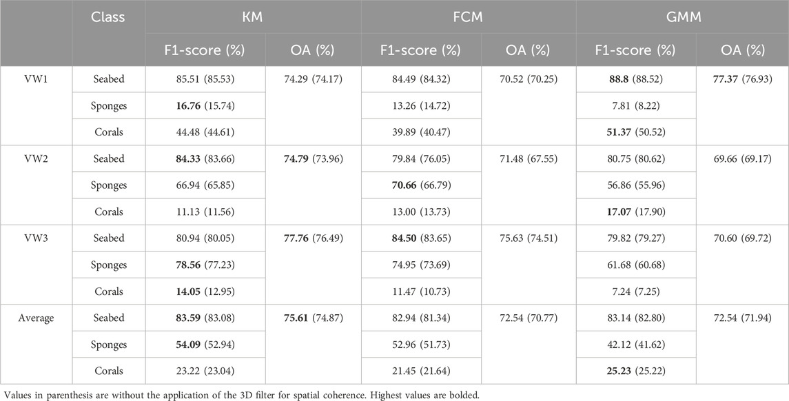
Table 3. Accuracy metrics (overall accuracy (OA) and F1-score) of the three vertical walls (VWs) from the three unsupervised classifiers (KM: K-Means, FCM: Fuzzy C-Means, and GMM: Gaussian Mixture Model).

Figure 5

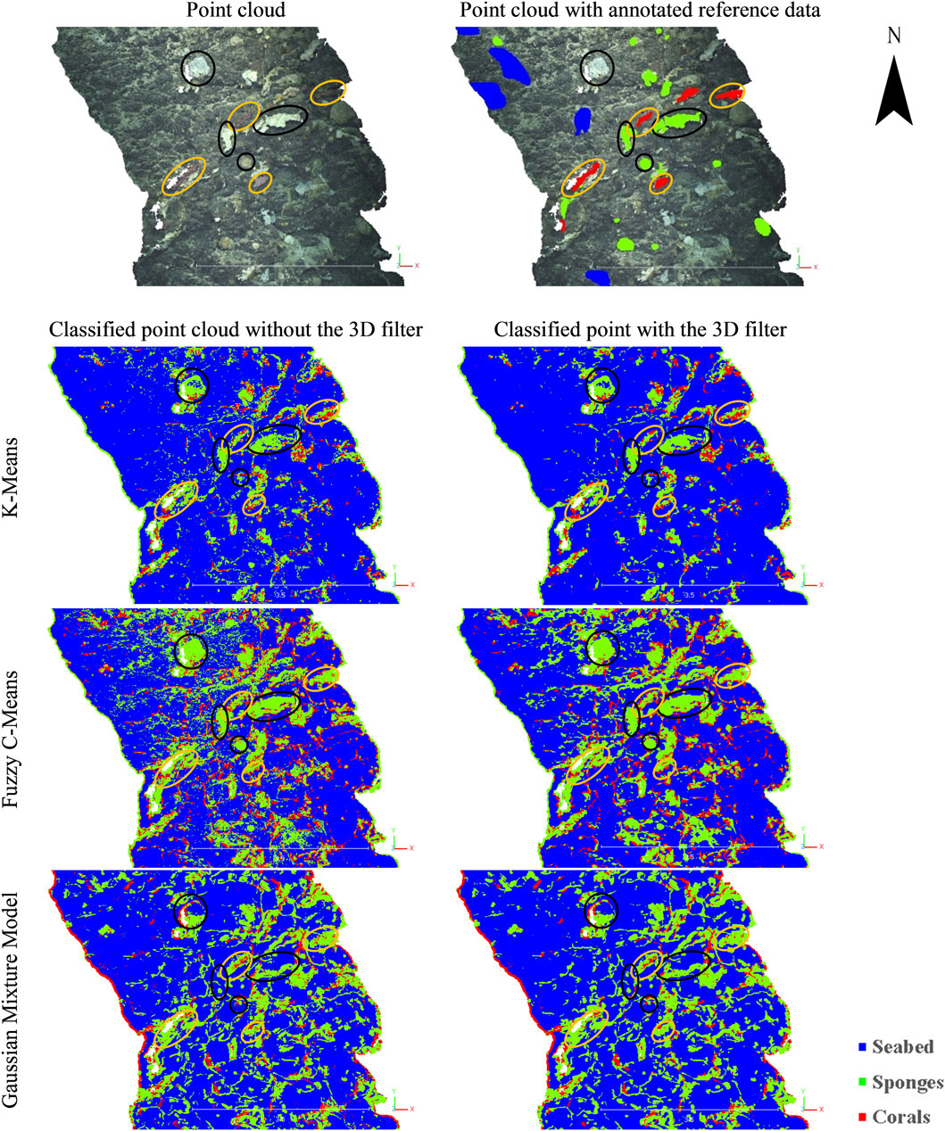
Figure 5. Portion of the classified point clouds from vertical wall 2 (VW2) based on the unsupervised classifiers before (left) and after (right) the application of the 3D filter. First row: Point cloud (left) and with annotated reference data (right). Examples of coral and sponge colonies are shown as orange and black ellipses, respectively.

3.2 Supervised ML classification

The RF classifier demonstrated the highest average OA of all walls with 84.50%, followed by LDA with 84.01%, and then DT with 79.90% (Table 4; Supplementary Table S2). Regarding the individual classes, LDA revealed the highest average F1-score, with 89.62%, 70.08%, and 43.79% for seabed, sponges, and corals, respectively. DT and RF correctly labeled most sponges and some corals (Figure 6; Supplementary Figure S3). However, DT produced noisy results, which reduced its overall performance. LDA misclassified some sponges as corals or seabed (black ellipses 2 and 3, respectively in Figure 6) and misclassified corals as sponges (Figure 6, orange ellipse a). The three classifiers failed in labeling some corals (Figure 6, orange ellipse b).

Table 4

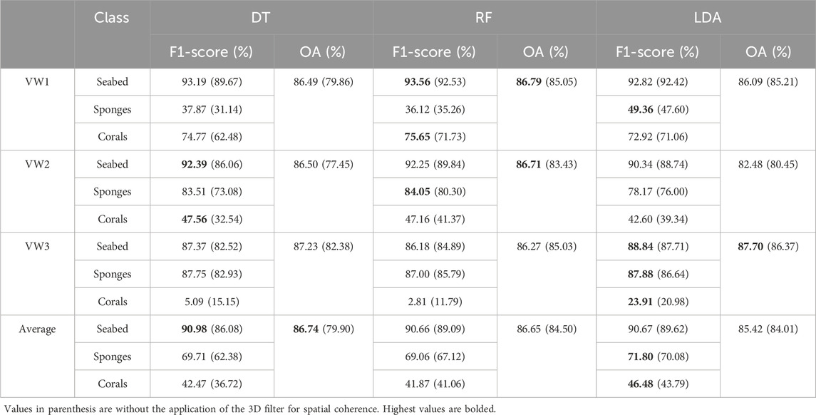
Table 4. Accuracy metrics (overall accuracy (OA) and F1-score) of the three vertical walls (VWs) from the three supervised classifiers (DT: Decision Tree, RF: Random Forest, and LDA: Linear Discriminant Analysis).

Figure 6

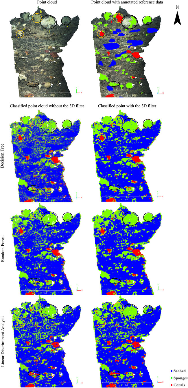
Figure 6. Portion of the classified point clouds from vertical wall 2 (VW2) based on the supervised classifiers before (left) and after (right) the application of the 3D filter. First row: Point cloud (left) and with annotated reference data (right). Examples of coral and sponge colonies are shown as orange ellipses (a, b) and black ellipses (1, 2 and 3), respectively. The point cloud in the orange ellipse “a” was correctly classified as corals using decision tree and random forest classifiers but misclassified as sponges using linear discriminant analysis. The point cloud in the orange ellipse “b” was misclassified as sponges by all classifiers. The point cloud in the black ellipse “1” was correctly classified as sponges by all classifiers. The point cloud in the black ellipses “2” and “3” were correctly classified as sponges using decision tree and random forest classifiers but misclassified as corals using linear discriminant analysis.

3.3 The impact of spatial coherence (3D filter)

The application of spatial coherence (3D filter) improved the accuracy and appearance of the results (Columns to the right of Figures 5, 6; Supplementary Figures S4, S5). The average overall classification accuracies increased by 0.6%–6.8%. For the unsupervised ML classification, the OA improved by less than 2%, except for the FCM classifier of VW2, which showed an improvement of about 4% (Table 3; Supplementary Table S3). However, this did not affect the ranking of the best-performing ML classifier overall or for individual classes. An improvement of the OA and F1-score was achieved for supervised ML classification, ranging from 1% to 4% from the RF and LDA classifiers (Table 4; Supplementary Table S4). LDA remained with the highest average F1-score for sponges and corals, but RF demonstrated the highest average F1-score for seabed with 90.98%. The most significant improvement following spatial filtering was observed with the DT classifier, particularly for VW2, which showed a 9% increase in OA and a 15% increase in F1-score for corals. This brought the performance of DT on par with the other two approaches. Increasing the search radius to 5 cm improved further the accuracy, but classes with low proportions, and smaller colonies, started to disappear.

3.4 Importance of color and geometric features

To investigate the impact of geometric features on classification performance, we compared the use of RGB features alone with nine geometric features using RF classifier for VW1 (from Dive 7) and VW2 (from Dive 9). The OA for VW2 was similar for both feature sets, with values of 70.26% for RGB features and 73.02% for the nine geometric features. In contrast, VW1 exhibited a substantial improvement, with an OA of 40.62% for RGB features and 77.40% for the nine geometric features. This disparity is further illustrated in the feature importance figure (Figure 7), which indicates that geometric features play a more significant role in the classification process for VW1 compared to VW2 and VW3.

Figure 7

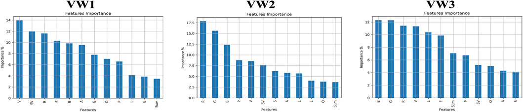
Figure 7. Features importance plots of the twelve features based on the random forest classifier for the three vertical walls (VWs). These features are Red (R), Green (G), Blue (B), linearity (L), planarity (P), sphericity (S), omni-variance (O), anisotropy (A), Eigen entropy (E), surface variation (SV), verticality (V), and sum.

The contribution of the twelve features to the classification process was computed based on the RF classifier (Figure 7). The classifier identified colors, as captured by RGB, to be most informative in assigning points to classes, particularly for VW2 and VW3. This is likely due to varying illumination of those walls compared to VW1 (see Figure 3). Following the RGB features, the most significant contributions came from verticality (V), surface variation (SV), sphericity (S), planarity (P), and linearity (L).

Planarity (P) was particularly successful at separating the seabed class, which was mainly considered a planar surface (Nanson et al., 2023) as opposed to coral and sponges, which showed higher surface variation (SV) (Díaz et al., 2023). Sphericity (S) helped detect sponges as many taxa (e.g., Geodia) exhibited spherical shapes (Santavy et al., 2013), while the verticality (V) feature mainly detected sponges (e.g., cup like and Hexactinellids) and corals (e.g., Plexauridae), which were naturally growing away from the wall (Kenchington et al., 2015). The linearity (L) feature detected other corals with branched shapes such as various species of the orders Antipatharia and Scleralcyonacea (Santavy et al., 2013).

4 Discussion

The 3D point clouds generated from underwater images provided a precise 3D representation of the seafloor habitat created by corals and sponges. These point clouds were analyzed based on their geometry using ML algorithms to categorize the seabed into ecologically meaningful classes representing taxa. We considered a wide range of ML algorithms with various clustering principles, including hard clustering (KM), soft clustering (FCM), and probabilistic clustering (GMM), as well as learning principles, including rule-based (DT), ensemble-based (RF), and probabilistic-based (LDA), to classify the underwater environment into three categories; seabed, sponges, and corals. The supervised ML classifiers achieved an average overall accuracy of 86.74%, 86.65%, and 85.42% from DT, RF, and LDA, respectively; while the unsupervised ML classifiers achieved an average overall accuracy of 75.61%, 72.54%, and 72.54% from KM, FCM, and GMM, respectively.

The supervised ML classifiers generally demonstrated higher accuracy metrics than the unsupervised classifiers. This is because the supervised ML classifiers rely on annotated points (i.e., training datasets) representing the actual classes to learn (Calvert et al., 2015). This is comparable with other studies which applied supervised ML classifiers (e.g., Mohamed et al., 2020; De Oliveira et al., 2021; De Oliveira et al., 2022). Of the unsupervised classifiers considered, KM demonstrated the highest OA for VW2 and VW3, while the GMM classifier revealed the highest OA for VW1. A higher percentage of sponges and corals were identified in VW2 and VW3, at 45% and 48%, respectively (see Table 1) leading to spherical clusters based on geometric features and RGB values. The KM algorithm is known to be particularly effective for identifying these types of clusters (Patel and Kushwaha, 2020; Mohamed et al., 2022; An et al., 2023), as also exemplified with our results. Conversely, GMM utilizes a probabilistic framework, which facilitates the handling of uncertainty and overlapping data points. This is relevant for VW1, where the seabed class dominated (∼71% of the data points), making GMM suitable for scenarios where data points may belong to multiple clusters (Patel and Kushwaha, 2020; An et al., 2023). In general, the KM classifier was fast and easy to implement and achieved good results compared to other unsupervised classifiers, especially FCM (Rong, 2011; Cebeci and Yildiz, 2015; Mohamed et al., 2022).

For the supervised classification, DT creates biased tree if some classes dominated (i.e., seabed in our case). This is attributed to DT’s aim to maximize node purity, leading to prioritization of the majority class. As a consequence, the tree may over-fit to the majority class, compromising its ability to effectively learn the decision boundaries for the minority classes, which in our case would be the ecologically important coral and sponge classes (Cieslak and Chawla, 2008; De Ville, 2013). On the other hand, RF fits several decision trees on various sub-samples of the dataset and uses averaging to improve the predictive accuracy and control over-fitting. LDA revealed the highest OA for VW3, but RF achieved highest OA for VW1 and VW2 and either close or higher F1-scores for individual classes. This suggests that RF might be more suitable for benthic classification than LDA or DT (Conti et al., 2019; Letard et al., 2021; De Oliveira et al., 2022). This may be because LDA assumes Gaussian distributions in the feature space, which cannot be guaranteed for the acquired data (Weinmann et al., 2015). In addition, the same covariance matrix is assumed for each class, and therefore only the means vary. Consequently, the LDA classifier has a conceptual limitation that may limit its application to benthic studies.

Incorporating geometric features in the classification process helped detect the 3D shapes of different corals and sponges (e.g., orange and black ellipses in Figure 8) and predict their distribution across the walls. Verticality (V), in specific, provides valuable insights into the structural characteristics of the seabed. For instance, corals typically exhibit a more vertical orientation due to their growth patterns, which is significantly different from the more horizontal or flat surfaces of the seabed (Kenchington et al., 2015). This distinction is crucial for accurate classification, as it allows for the identification of coral reefs, which are vital ecosystems. Additionally, sponges may display varying degrees of verticality depending on their species and growth conditions (Santavy et al., 2013). By using verticality, ML models can better classify these organisms based on their structural features, thus enhancing the overall accuracy of seabed classification efforts.

Figure 8

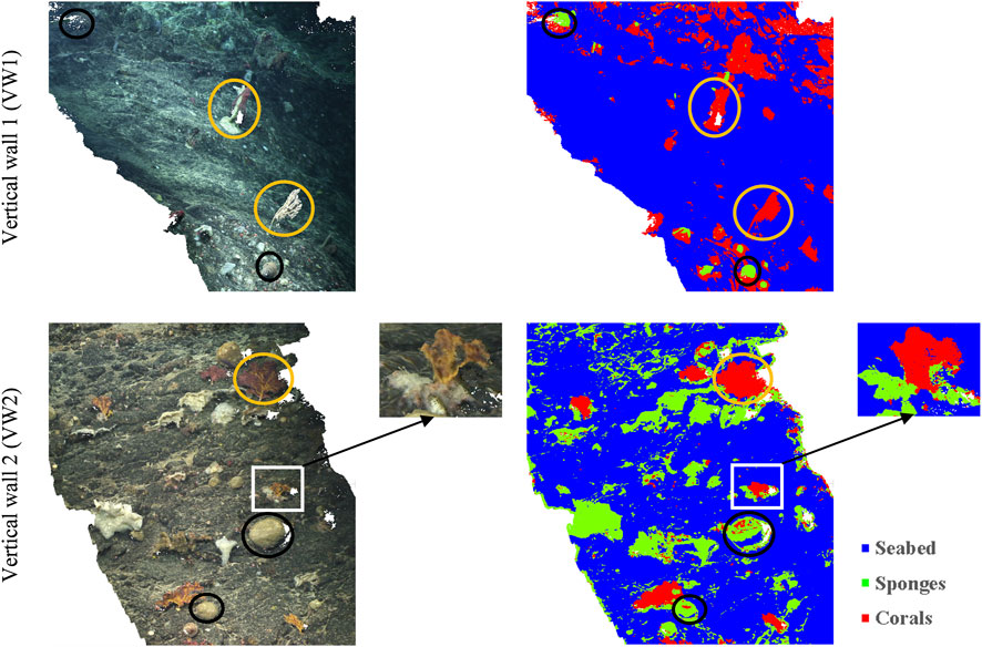
Figure 8. Examples of classified point clouds using random forest with the 3D filter. Examples of 3D corals and sponges are shown in orange and black ellipses, respectively. The point cloud in the white box shows correctly classified corals over sponges.

The full coverage predictions showed variation across space, with corals tending to be distributed in the northern and southeren portions of VW1. On the other hand, dense sponges’ aggregations were located in the northern and western areas of VW2 and VW3, respectively. Sparse areas of sponges and corals were observed in VW1 and VW2/VW3, respectively (Figure 9). The highest proportion class (i.e., seabed) represented in the reference data generally had the highest classification scores, except for VW3, where the recall and F1-score of sponges were also high. VW3 was the wall with the highest representation of sponges in the annotation data. The F1-score for corals, on the other hand, was the lowest, which may be partly due to their more variable morphology and size, as well as lower coverage compared to sponges and seabed classes.

Figure 9

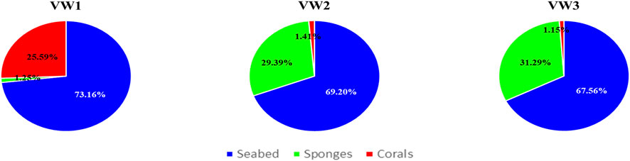
Figure 9. Predicted percentage cover of each class for all vertical walls based on the best classifier (random forest for vertical wall 1 (VW1) and VW2, and linear discriminant analysis for VW3).

Although relatively high OAs were achieved for all walls, the presented work suffers from the limitations of underwater imagery (O’Byrne et al., 2018). Inadequate illumination and variable water turbidity caused poor image quality in certain areas. This is obvious from the 3D point reconstruction of different walls, where VW1 exhibited a colder color, and VW3 exhibited a warmer color (Figure 3). VW2 showed the lowest OA using unsupervised or supervised ML classifiers among the three tested walls. This is most likely the results of varying illumination along the wall, with the southern section being significantly darker than the northern section. The variable water properties also caused low contrast and color distortion, leading to occasional blurred images (Lu et al., 2015). Currents may also cause benthic habitats to appear differently from various camera angles (Lim et al., 2020). This can be particularly problematic when studying cold-water corals on vertical walls as these corals tend to prefer high-current areas where the complex topography is likely to interact with local currents (Robert et al., 2020). Thus, future studies should consider RGB values correction and/or image enhancement to improve the contrast of underwater habitats (Han et al., 2018). Promising avenues include enhancing underwater images by removing the attenuation effects (Akkaynak and Treibitz, 2019; Zhang et al., 2022), color restoration by estimating of both light conditions and the optical properties of the medium (water) in real-time (Nakath et al., 2021), and combining a physical imaging formation model with a multiscale deep neural network to enhance underwater image quality (Li et al., 2022).

Several studies have evaluated deep learning models for seabed classification of 2D imagery (Jackett et al., 2023; Prado et al., 2023; Lowe et al., 2025) or shallow-water coral data (Hopkinson et al., 2020). These models have demonstrated superior generalization capabilities (Schürholz and Chennu, 2023). However, their application in seabed classification presents significant challenges, primarily due to the need for extensive labeled datasets (Wan et al., 2022). While powerful in capturing complex patterns, these models require a substantial investment of time and resources in the labeling process, which is often labor-intensive and demands expert knowledge to ensure accuracy (Garone et al., 2023). This barrier can limit the feasibility of implementing deep learning techniques in deep-sea settings where such comprehensive datasets are not readily available (Wan et al., 2022).

In our research, we focused on evaluating the effectiveness of using geometric features with RGB based on existing supervised and unsupervised classification models before considering the adoption of more complex architectures, such as convolutional neural networks (Hopkinson et al., 2020; Loureiro et al., 2024). Future studies may benefit from exploring the integration of deep learning models to leverage geometric features for enhanced classification accuracy.

5 Conclusion

The recent development of SfM significantly increases our ability to map at very high-resolution deep-sea environments using simple cameras mounted on ROVs, yet its application for seafloor and taxa classification has remained limited. One of the advantages of using 3D point clouds for seafloor classification is that they provide a more detailed and accurate representation of complex structures, from which quantitative measures such as volume–and with the addition of samples, eventually biomass–can be derived. In addition, the use of SfM point clouds can also be achieved from archival imagery (Bennecke et al., 2016) while the use of ML algorithms considerably lowered the exhaustive manual annotation process of underwater imagery. Generally, the supervised ML classifiers outperformed the unsupervised ML classifiers, with RF demonstrating more consistent results than all other classifiers except for LDA for certain individual classes. As such, future investigations could investigate combining two or more classifiers to maximize their usefulness.

3D point clouds created highly detailed visualizations of the seafloor that can help understand the geology and ecology of the ocean floor and assess the health of marine ecosystems by enabling quantitative measurements over time. This information is crucial for understanding the response of ecosystems to climate change and sustainably managing our oceans. The presented classification methods could help track the spatial distribution of corals and sponges more efficiently in the future, aiding in conservation efforts and monitoring of Marine Protected Areas.

Data availability statement

The raw data supporting the conclusions of this article will be made available by the authors, without undue reservation.

Author contributions

SM: Conceptualization, Data curation, Formal Analysis, Investigation, Methodology, Software, Validation, Visualization, Writing – original draft, Writing – review and editing. AY-S: Data curation, Methodology, Visualization, Writing – review and editing. KR: Conceptualization, Funding acquisition, Methodology, Project administration, Resources, Supervision, Writing – review and editing, Writing – original draft.

Funding

The authors declare that financial support was received for the research and/or publication of this article. Data were collected during the TOSCA expedition (Marine Institute, Ireland) onboard the RV Celtic Explorer. Research funding was provided by the Ocean Frontier Institute, through an award from the Canada First Research Excellence Fund as part of the project “Benthic Ecosystem Mapping and Engagement” (BEcoME). Further funding was provided by a Canada Research Chair in Ocean Mapping and A-B. Yanez-Suarez was supported by an “Natural Sciences and Engineering Research Council” Discovery Grant to PI Katleen Robert.

Conflict of interest

The authors declare that the research was conducted in the absence of any commercial or financial relationships that could be construed as a potential conflict of interest.

Generative AI statement

The authors declare that no Generative AI was used in the creation of this manuscript.

Any alternative text (alt text) provided alongside figures in this article has been generated by Frontiers with the support of artificial intelligence and reasonable efforts have been made to ensure accuracy, including review by the authors wherever possible. If you identify any issues, please contact us.

Publisher’s note

All claims expressed in this article are solely those of the authors and do not necessarily represent those of their affiliated organizations, or those of the publisher, the editors and the reviewers. Any product that may be evaluated in this article, or claim that may be made by its manufacturer, is not guaranteed or endorsed by the publisher.

Supplementary material

The Supplementary Material for this article can be found online at: https://www.frontiersin.org/articles/10.3389/frsen.2025.1680353/full#supplementary-material

References

Agisoft (2020). Agisoft metashape. Available online at: https://www.agisoft.com.

Google Scholar

Akkaynak, D., and Treibitz, T. (2019). “Sea-thru: a method for removing water from underwater images,” in Proceedings of the IEEE/CVF conference on computer vision and pattern recognition, 1682–1691.

Google Scholar

Alt, C. H., Kremenetskaia, A., Gebruk, A. V., Gooday, A. J., and Jones, D. O. (2019). Bathyal benthic megafauna from the mid-atlantic ridge in the region of the charlie-gibbs fracture zone based on remotely operated vehicle observations. Deep Sea Res. Part I Oceanogr. Res. Pap. 145, 1–12. doi:10.1016/j.dsr.2018.12.006

CrossRef Full Text | Google Scholar

An, Q., Rahman, S., Zhou, J., and Kang, J. J. (2023). A comprehensive review on machine learning in healthcare industry: classification, restrictions, opportunities and challenges. Sensors 23 (9), 4178. doi:10.3390/s23094178

PubMed Abstract | CrossRef Full Text | Google Scholar

Bennecke, S., Kwasnitschka, T., Metaxas, A., and Dullo, W. C. (2016). In situ growth rates of deep-water octocorals determined from 3D photogrammetric reconstructions. Coral Reefs 35, 1227–1239. doi:10.1007/s00338-016-1471-7

CrossRef Full Text | Google Scholar

Bezdek, J. C., Ehrlich, R., and Full, W. (1984). FCM: the fuzzy c-means clustering algorithm. Comput. and geosciences 10 (2-3), 191–203. doi:10.1016/0098-3004(84)90020-7

CrossRef Full Text | Google Scholar

Blender Foundation (2021). Blender. Available online at: https://www.blender.org/download/releases/2-92.

Google Scholar

Breiman, L. (2001). Random forests. Mach. Learn. 45, 5–32. doi:10.1023/a:1010933404324

CrossRef Full Text | Google Scholar

Brown, C. J., Sameoto, J. A., and Smith, S. J. (2012). Multiple methods, maps, and management applications: purpose made seafloor maps in support of ocean management. J. Sea Res. 72, 1–13. doi:10.1016/j.seares.2012.04.009

CrossRef Full Text | Google Scholar

Calvert, A. J., and Whitmarsh, R. B. (1986). The structure of the Charlie–Gibbs Fracture zone. J. Geol. Soc. 143 (5), 819–821. doi:10.1144/gsjgs.143.5.0819

CrossRef Full Text | Google Scholar

Calvert, J., Strong, J. A., Service, M., McGonigle, C., and Quinn, R. (2015). An evaluation of supervised and unsupervised classification techniques for marine benthic habitat mapping using multibeam echosounder data. ICES J. Mar. Sci. 72 (5), 1498–1513. doi:10.1093/icesjms/fsu223

CrossRef Full Text | Google Scholar

Cathalot, C., Van Oevelen, D., Cox, T. J., Kutti, T., Lavaleye, M., Duineveld, G., et al. (2015). Cold-water coral reefs and adjacent sponge grounds: hotspots of benthic respiration and organic carbon cycling in the deep sea. Front. Mar. Sci. 2, 37. doi:10.3389/fmars.2015.00037

CrossRef Full Text | Google Scholar

Cebeci, Z., and Yildiz, F. (2015). Comparison of k-means and fuzzy c-means algorithms on different cluster structures. J. Agric. Inf. 6 (3). doi:10.17700/jai.2015.6.3.196

CrossRef Full Text | Google Scholar

Cieslak, D. A., and Chawla, N. V. (2008). “Learning decision trees for unbalanced data,”Mach. Learn. Knowl. Discov. Databases Eur. Conf. ECML PKDD 2008, Antwerp, Belg. Sept. 15-19, 2008, Proc. Part I, 19. 241–256. doi:10.1007/978-3-540-87479-9_34

CrossRef Full Text | Google Scholar

CloudCompare (2022). CloudCompare. Available online at: https://www.cloudcompare.org/.

Google Scholar

Coates, A., and Ng, A. Y. (2012). “Learning feature representations with k-means,” in Neural networks: tricks of the trade. Second Edition (Berlin, Heidelberg: Springer Berlin Heidelberg), 561–580.

CrossRef Full Text | Google Scholar

Congalton, R. G. (1991). A review of assessing the accuracy of classifications of remotely sensed data. Remote Sens. Environ. 37 (1), 35–46. doi:10.1016/0034-4257(91)90048-b

CrossRef Full Text | Google Scholar

Conti, L. A., Lim, A., and Wheeler, A. J. (2019). High resolution mapping of a cold water coral mound. Sci. Rep. 9 (1), 1016. doi:10.1038/s41598-018-37725-x

PubMed Abstract | CrossRef Full Text | Google Scholar

De Oliveira, L. M. C., Lim, A., Conti, L. A., and Wheeler, A. J. (2021). 3D classification of cold-water coral reefs: a comparison of classification techniques for 3D reconstructions of cold-water coral reefs and seabed. Front. Mar. Sci. 8, 640713. doi:10.3389/fmars.2021.640713

CrossRef Full Text | Google Scholar

De Oliveira, L. M. C., Lim, A., Conti, L. A., and Wheeler, A. J. (2022). High-resolution 3D mapping of cold-water coral reefs using machine learning. Front. Environ. Sci. 10, 1044706. doi:10.3389/fenvs.2022.1044706

CrossRef Full Text | Google Scholar

De Ville, B. (2013). Decision trees. Wiley Interdiscip. Rev. Comput. Stat. 5 (6), 448–455. doi:10.1002/wics.1278

CrossRef Full Text | Google Scholar

Demantké, J., Vallet, B., and Paparoditis, N. (2012). Streamed vertical rectangle detection in terrestrial laser scans for facade database production. ISPRS Ann. Photogramm. Remote Sens. Spat. Inf. Sci. 1 (September), 99–104. doi:10.5194/isprsannals-I-3-99-2012

CrossRef Full Text | Google Scholar

Díaz, M. C., Nuttall, M., Pomponi, S. A., Rützler, K., Klontz, S., Adams, C., et al. (2023). An annotated and illustrated identification guide to common mesophotic reef sponges (Porifera, Demospongiae, Hexactinellida, and Homoscleromorpha) inhabiting flower garden banks national marine sanctuary and vicinities. ZooKeys 1161, 1–68. doi:10.3897/zookeys.1161.93754

PubMed Abstract | CrossRef Full Text | Google Scholar

Elberink, S. O., and Maas, H. G. (2000). The use of anisotropic height texture measures for the segmentation of airborne laser scanner data. Int. archives photogrammetry remote Sens. 33, 678–684.

Google Scholar

Garone, R. V., Birkenes Lønmo, T. I., Schimel, A. C. G., Diesing, M., Thorsnes, T., and Løvstakken, L. (2023). Seabed classification of multibeam echosounder data into bedrock/non-bedrock using deep learning. Front. Earth Sci. 11, 1285368. doi:10.3389/feart.2023.1285368

CrossRef Full Text | Google Scholar

Goutte, C., and Gaussier, E. (2005). “A probabilistic interpretation of precision, recall and F-score, with implication for evaluation,”Adv. Inf. Retr. 27th Eur. Conf. IR Res. ECIR 2005, Santiago de Compostela, Spain, March 21-23, 2005, 27. 345–359. doi:10.1007/978-3-540-31865-1_25

CrossRef Full Text | Google Scholar

Hackel, T., Wegner, J. D., and Schindler, K. (2016). Fast semantic segmentation of 3D point clouds with strongly varying density. ISPRS Ann. photogrammetry, remote Sens. spatial Inf. Sci. 3, 177–184. doi:10.5194/isprsannals-iii-3-177-2016

CrossRef Full Text | Google Scholar

Han, M., Lyu, Z., Qiu, T., and Xu, M. (2018). A review on intelligence dehazing and color restoration for underwater images. IEEE Trans. Syst. Man, Cybern. Syst. 50 (5), 1820–1832. doi:10.1109/tsmc.2017.2788902

CrossRef Full Text | Google Scholar

He, X., Cai, D., Shao, Y., Bao, H., and Han, J. (2010). Laplacian regularized gaussian mixture model for data clustering. IEEE Trans. Knowl. Data Eng. 23 (9), 1406–1418. doi:10.1109/tkde.2010.259

CrossRef Full Text | Google Scholar

Henry, L. A., and Roberts, J. M. (2017). “Global biodiversity in cold-water coral reef ecosystems,” in Marine animal forests: the ecology of benthic biodiversity hotspots, 235–256.

Google Scholar

Hopkinson, B. M., King, A. C., Owen, D. P., Johnson-Roberson, M., Long, M. H., and Bhandarkar, S. M. (2020). Automated classification of three-dimensional reconstructions of coral reefs using convolutional neural networks. PloS one 15 (3), e0230671. doi:10.1371/journal.pone.0230671

PubMed Abstract | CrossRef Full Text | Google Scholar

Jackett, C., Althaus, F., Maguire, K., Farazi, M., Scoulding, B., Untiedt, C., et al. (2023). A benthic substrate classification method for seabed images using deep learning: application to management of deep-sea coral reefs. J. Appl. Ecol. 60 (7), 1254–1273. doi:10.1111/1365-2664.14408

CrossRef Full Text | Google Scholar

Jutzi, B., and Gross, H. (2009). Nearest neighbour classification on laser point clouds to gain object structures from buildings. Int. Archives Photogrammetry, Remote Sens. Spatial Inf. Sci. 38 (Part 1), 4–7.

Google Scholar

Kenchington, E., Beazley, L., Murillo, F. J., Tompkins MacDonald, G., and Baker, E. (2015). Coral, sponge, and other vulnerable marine ecosystem indicator identification guide, NAFO area. NAFO Scientific Council Studies, Nova Scotia.

Google Scholar

Keogh, P., Command, R. J., Edinger, E., Georgiopoulou, A., and Robert, K. (2022). Benthic megafaunal biodiversity of the Charlie-Gibbs fracture zone: spatial variation, potential drivers, and conservation status. Mar. Biodivers. 52 (5), 55–18. doi:10.1007/s12526-022-01285-1

PubMed Abstract | CrossRef Full Text | Google Scholar

Letard, M., Collin, A., Corpetti, T., Lague, D., Pastol, Y., and Mury, A. (2021). “Classification of coastal and estuarine ecosystems using full-waveform topo-bathymetric lidar data and artificial intelligence,” in Oceans 2021: san diego–porto (IEEE), 1–10.

CrossRef Full Text | Google Scholar

Letard, M., Collin, A., Corpetti, T., Lague, D., Pastol, Y., and Ekelund, A. (2022). Classification of land-water continuum habitats using exclusively airborne topobathymetric LiDAR green waveforms and infrared intensity point clouds. Remote Sens. 14 (2), 341. doi:10.3390/rs14020341

CrossRef Full Text | Google Scholar

Li, F., Lu, D., Lu, C., and Jiang, Q. (2022). Underwater imaging Formation model-embedded multiscale deep neural network for underwater image enhancement. Math. Problems Eng. 2022 (1), 1–11. doi:10.1155/2022/8330985

CrossRef Full Text | Google Scholar

Liang, H., Li, N., and Zhao, S. (2021). Salt and pepper noise removal method based on a detail-aware filter. Symmetry 13 (3), 515. doi:10.3390/sym13030515

CrossRef Full Text | Google Scholar

Lim, A., Wheeler, A. J., Price, D. M., O’Reilly, L., Harris, K., and Conti, L. (2020). Influence of benthic currents on cold-water coral habitats: a combined benthic monitoring and 3D photogrammetric investigation. Sci. Rep. 10 (1), 19433. doi:10.1038/s41598-020-76446-y

PubMed Abstract | CrossRef Full Text | Google Scholar

Loureiro, G., Dias, A., Almeida, J., Martins, A., Hong, S., and Silva, E. (2024). A survey of seafloor characterization and mapping techniques. Remote Sens. 16 (7), 1163. doi:10.3390/rs16071163

CrossRef Full Text | Google Scholar

Lowe, S. C., Misiuk, B., Xu, I., Abdulazizov, S., Baroi, A. R., Bastos, A. C., et al. (2025). BenthicNet: a global compilation of seafloor images for deep learning applications. Sci. Data 12 (1), 230. doi:10.1038/s41597-025-04491-1

PubMed Abstract | CrossRef Full Text | Google Scholar

Lu, H., Li, Y., Zhang, L., and Serikawa, S. (2015). Contrast enhancement for images in turbid water. J. Opt. Soc. Am. A 32 (5), 886–893. doi:10.1364/josaa.32.000886

PubMed Abstract | CrossRef Full Text | Google Scholar

Lucieer, V., and Lamarche, G. (2011). Unsupervised fuzzy classification and object-based image analysis of multibeam data to map deep water substrates, Cook Strait, New Zealand. Cont. Shelf Res. 31 (11), 1236–1247. doi:10.1016/j.csr.2011.04.016

CrossRef Full Text | Google Scholar

MacQueen, J. (1967). “Classification and analysis of multivariate observations,” in 5th Berkeley symp. Math. Statist. Probability (Los Angeles LA USA: University of California), 281–297.

Google Scholar

Mahmood, A., Bennamoun, M., An, S., Sohel, F. A., Boussaid, F., Hovey, R., et al. (2018). Deep image representations for coral image classification. IEEE J. Ocean. Eng. 44 (1), 121–131. doi:10.1109/joe.2017.2786878

CrossRef Full Text | Google Scholar

Mahmood, A., Ospina, A. G., Bennamoun, M., An, S., Sohel, F., Boussaid, F., et al. (2020). Automatic hierarchical classification of kelps using deep residual features. Sensors 20 (2), 447. doi:10.3390/s20020447

PubMed Abstract | CrossRef Full Text | Google Scholar

Marcillat, M., Van Audenhaege, L., Borremans, C., Arnaubec, A., and Menot, L. (2024). The best of two worlds: reprojecting 2D image annotations onto 3D models. PeerJ 12, e17557. doi:10.7717/peerj.17557

PubMed Abstract | CrossRef Full Text | Google Scholar

Marutho, D., Handaka, S. H., and Wijaya, E. (2018). “The determination of cluster number at k-mean using elbow method and purity evaluation on headline news,” in 2018 international seminar on application for technology of information and communication (IEEE), 533–538.

Google Scholar

Mather, P., and Tso, B. (2016). Classification methods for remotely sensed data. Boca Raton, FL, United States: CRC Press. doi:10.1201/9781420090741

CrossRef Full Text | Google Scholar

Maugis, C., Celeux, G., and Martin-Magniette, M. L. (2009). Variable selection for clustering with Gaussian mixture models. Biometrics 65 (3), 701–709. doi:10.1111/j.1541-0420.2008.01160.x

PubMed Abstract | CrossRef Full Text | Google Scholar

McGeady, R., Runya, R. M., Dooley, J. S., Howe, J. A., Fox, C. J., Wheeler, A. J., et al. (2023). A review of new and existing non-extractive techniques for monitoring marine protected areas. Front. Mar. Sci. 10, 1126301. doi:10.3389/fmars.2023.1126301

CrossRef Full Text | Google Scholar

Mohamed, H., Nadaoka, K., and Nakamura, T. (2018). Assessment of machine learning algorithms for automatic benthic cover monitoring and mapping using towed underwater video camera and high-resolution satellite images. Remote Sens. 10 (5), 773. doi:10.3390/rs10050773

CrossRef Full Text | Google Scholar

Mohamed, H., Nadaoka, K., and Nakamura, T. (2020). Towards benthic habitat 3D mapping using machine learning algorithms and structures from motion photogrammetry. Remote Sens. 12 (1), 127. doi:10.3390/rs12010127

CrossRef Full Text | Google Scholar

Mohamed, M., Morsy, S., and El-Shazly, A. (2021). Evaluation of data subsampling and neighbourhood selection for mobile LiDAR data classification. Egypt. J. Remote Sens. Space Sci. 24 (3), 799–804. doi:10.1016/j.ejrs.2021.04.003

CrossRef Full Text | Google Scholar

Mohamed, H., Nadaoka, K., and Nakamura, T. (2022). Automatic semantic segmentation of benthic habitats using images from towed underwater camera in a complex shallow water environment. Remote Sens. 14 (8), 1818. doi:10.3390/rs14081818

CrossRef Full Text | Google Scholar

Morato, T., González-Irusta, J. M., Dominguez-Carrió, C., Wei, C. L., Davies, A., Sweetman, A. K., et al. (2020). Climate-induced changes in the suitable habitat of cold-water corals and commercially important deep-sea fishes in the North Atlantic. Glob. Change Biol. 26 (4), 2181–2202. doi:10.1111/gcb.14996

PubMed Abstract | CrossRef Full Text | Google Scholar

Morsy, S., and Shaker, A. (2022). Evaluation of LiDAR-Derived features relevance and training data minimization for 3D point cloud classification. Remote Sens. 14 (23), 5934. doi:10.3390/rs14235934

CrossRef Full Text | Google Scholar

Mortensen, P. B., Buhl-Mortensen, L., Gebruk, A. V., and Krylova, E. M. (2008). Occurrence of deep-water corals on the Mid-Atlantic Ridge based on MAR-ECO data. Deep Sea Res. Part II Top. Stud. Oceanogr. 55 (1-2), 142–152. doi:10.1016/j.dsr2.2007.09.018

CrossRef Full Text | Google Scholar

Nakath, D., She, M., Song, Y., and Köser, K. (2021). “In-situ joint light and medium estimation for underwater color restoration,” in Proceedings of the IEEE/CVF international conference on computer vision, 3731–3740.

Google Scholar

Nanson, R., Arosio, R., Gafeira, J., McNeil, M., Dove, D., Bjarnadóttir, L., et al. (2023). “A two-part seabed geomorphology classification scheme,” in Part 2: geomorphology classification framework and glossary.

Google Scholar

OSPAR (2010). OSPAR decision 2010/2 on the establishment of the charlie-Gibbs South Marine protected area, 1–5.

Google Scholar

OSPAR (2012). OSPAR decision 2012/1 on the establishment of the charlie-gibbs north high Seas marine protected area, 1–5.

Google Scholar

O’Byrne, M., Schoefs, F., Pakrashi, V., and Ghosh, B. (2018). An underwater lighting and turbidity image repository for analysing the performance of image-based non-destructive techniques. Struct. Infrastructure Eng. 14 (1), 104–123. doi:10.1080/15732479.2017.1330890

CrossRef Full Text | Google Scholar

Parrish, C. E., Dijkstra, J. A., O'Neil-Dunne, J. P., McKenna, L., and Pe'eri, S. (2016). Post-Sandy benthic habitat mapping using new topobathymetric lidar technology and object-based image classification. J. Coast. Res. 76 (10076), 200–208. doi:10.2112/si76-017

CrossRef Full Text | Google Scholar

Patel, E., and Kushwaha, D. S. (2020). Clustering cloud workloads: K-means vs gaussian mixture model. Procedia Comput. Sci. 171, 158–167. doi:10.1016/j.procs.2020.04.017

CrossRef Full Text | Google Scholar

Pauly, M., Keiser, R., and Gross, M. (2003). “Multi-scale feature extraction on point-sampled surfaces,”Comput. Graph. forum, 22, 281–289. doi:10.1111/1467-8659.00675

CrossRef Full Text | Google Scholar

Pedregosa, F., Varoquaux, G., Gramfort, A., Michel, V., Thirion, B., Grisel, O., et al. (2011). Scikit-learn: machine learning in Python. J. Mach. Learn. Res. 12 (Oct), 2825–2830.

Google Scholar

Piazza, P., Cummings, V., Guzzi, A., Hawes, I., Lohrer, A., Marini, S., et al. (2019). Underwater photogrammetry in Antarctica: Long-term observations in benthic ecosystems and legacy data rescue. Polar Biol. 42 (6), 1061–1079. doi:10.1007/s00300-019-02480-w

CrossRef Full Text | Google Scholar

Pierce, J., Butler IV, M. J., Rzhanov, Y., Lowell, K., and Dijkstra, J. A. (2021). Classifying 3-D models of coral reefs using structure-from-motion and multi-view semantic segmentation. Front. Mar. Sci. 1623. doi:10.3389/fmars.2021.706674

CrossRef Full Text | Google Scholar

Prado, E., Abad-Uribarren, A., Ramo, R., Sierra, S., González-Pola, C., Cristobo, J., et al. (2023). Describing polyps behavior of a deep-sea gorgonian, Placogorgia sp., using a deep-learning approach. Remote Sens. 15 (11), 2777. doi:10.3390/rs15112777

CrossRef Full Text | Google Scholar

Price, D. M., Robert, K., Callaway, A., Hall, R. A., and Huvenne, V. A. (2019). Using 3D photogrammetry from ROV video to quantify cold-water coral reef structural complexity and investigate its influence on biodiversity and community assemblage. Coral Reefs 38 (5), 1007–1021. doi:10.1007/s00338-019-01827-3

CrossRef Full Text | Google Scholar

Price, D. M., Lim, A., Callaway, A., Eichhorn, M. P., Wheeler, A. J., Lo Iacono, C., et al. (2021). Fine-scale heterogeneity of a cold-water coral reef and its influence on the distribution of associated taxa. Front. Mar. Sci. 218, 556313. doi:10.3389/fmars.2021.556313

CrossRef Full Text | Google Scholar

Quinlan, J. R. (1986). Induction of decision trees. Mach. Learn. 1, 81–106. doi:10.1023/a:1022643204877

CrossRef Full Text | Google Scholar

Ragnarsson, S. Á., Burgos, J. M., Kutti, T., van den Beld, I., Egilsdóttir, H., Arnaud-Haond, S., et al. (2017). “The impact of anthropogenic activity on cold-water corals,” in Marine animal forests: the ecology of benthic biodiversity hotspots, 989–1023.

Google Scholar

Robert, K., Huvenne, V. A., Georgiopoulou, A., Jones, D. O., Marsh, L., Do Carter, G., et al. (2017). New approaches to high-resolution mapping of marine vertical structures. Sci. Rep. 7 (1), 9005. doi:10.1038/s41598-017-09382-z

PubMed Abstract | CrossRef Full Text | Google Scholar

Robert, K., Jones, D. O., Georgiopoulou, A., and Huvenne, V. A. (2020). Cold-water coral assemblages on vertical walls from the Northeast Atlantic. Divers. Distributions 26 (3), 284–298. doi:10.1111/ddi.13011

CrossRef Full Text | Google Scholar

Rong, C. (2011). “Using Mahout for clustering Wikipedia's latest articles: a comparison between k-means and fuzzy c-means in the cloud,” in 2011 IEEE third international conference on cloud computing technology and science (IEEE), 565–569.

Google Scholar

Rovers, A., De Vreede, I., Rook, M., Psomadaki, S., Nagelkerke, T., and Verbree, E. (2015). Semantically enriching point clouds: the case of street levels. Geomatics Synth. Proj. 2015/16.

Google Scholar

Santavy, D. L., Courtney, L. A., Fisher, W. S., Quarles, R. L., and Jordan, S. J. (2013). Estimating surface area of sponges and gorgonians as indicators of habitat availability on Caribbean coral reefs. Hydrobiologia 707 (1), 1–16. doi:10.1007/s10750-012-1359-7

CrossRef Full Text | Google Scholar

Schürholz, D., and Chennu, A. (2023). Digitizing the coral reef: machine learning of underwater spectral images enables dense taxonomic mapping of benthic habitats. Methods Ecol. Evol. 14 (2), 596–613. doi:10.1111/2041-210x.14029

CrossRef Full Text | Google Scholar

Skolotnev, S., Sanfilippo, A., Peyve, A., Nestola, Y., Sokolov, S., and Ligi, M. (2021). Seafloor spreading and tectonics at the Charlie gibbs transform System (52-53°N, Mid Atlantic Ridge): preliminary results from R/V AN strakhov expedition S50. Ofioliti. doi:10.4454/ofioliti.v46i1.539

CrossRef Full Text | Google Scholar

Soetaert, K., Mohn, C., Rengstorf, A., Grehan, A., and van Oevelen, D. (2016). Ecosystem engineering creates a direct nutritional link between 600-m deep cold-water coral mounds and surface productivity. Sci. Rep. 6 (1), 35057. doi:10.1038/srep35057

PubMed Abstract | CrossRef Full Text | Google Scholar

Talukder, B., Ganguli, N., Matthew, R., Hipel, K. W., and Orbinski, J. (2022). Climate change-accelerated ocean biodiversity loss and associated planetary health impacts. J. Clim. Change Health 6, 100114. doi:10.1016/j.joclim.2022.100114

CrossRef Full Text | Google Scholar

Ternon, Q., Danet, V., Thiriet, P., Ysnel, F., Feunteun, E., and Collin, A. (2022). Classification of underwater photogrammetry data for temperate benthic rocky reef mapping. Estuar. Coast. Shelf Sci. 270, 107833. doi:10.1016/j.ecss.2022.107833

CrossRef Full Text | Google Scholar

Thomas, H., Goulette, F., Deschaud, J. E., Marcotegui, B., and LeGall, Y. (2018). “Semantic classification of 3D point clouds with multiscale spherical neighborhoods,” in 2018 International conference on 3D vision (3DV) (IEEE), 390–398.

CrossRef Full Text | Google Scholar

Titschack, J., Fink, H. G., Baum, D., Wienberg, C., Hebbeln, D., and Freiwald, A. (2016). Mediterranean cold-water corals–an important regional carbonate factory? Depositional Rec. 2 (1), 74–96. doi:10.1002/dep2.14

CrossRef Full Text | Google Scholar

Ventura, D., Grosso, L., Pensa, D., Casoli, E., Mancini, G., Valente, T., et al. (2023). Coastal benthic habitat mapping and monitoring by integrating aerial and water surface low-cost drones. Front. Mar. Sci. 9, 1096594. doi:10.3389/fmars.2022.1096594

CrossRef Full Text | Google Scholar

Waldhauser, C., Hochreiter, R., Otepka, J., Pfeifer, N., Ghuffar, S., Korzeniowska, K., et al. (2014). “Automated classification of airborne laser scanning point clouds,” in Solving computationally expensive engineering problems: methods and applications (Springer International Publishing), 269–292.

CrossRef Full Text | Google Scholar

Wan, J., Qin, Z., Cui, X., Yang, F., Yasir, M., Ma, B., et al. (2022). MBES seabed sediment classification based on a decision fusion method using deep learning model. Remote Sens. 14 (15), 3708. doi:10.3390/rs14153708

CrossRef Full Text | Google Scholar

Weinmann, M., Jutzi, B., and Mallet, C. (2014). Semantic 3D scene interpretation: a framework combining optimal neighborhood size selection with relevant features. ISPRS Ann. Photogrammetry, Remote Sens. Spatial Inf. Sci. 2 (3), 181–188. doi:10.5194/isprsannals-ii-3-181-2014

CrossRef Full Text | Google Scholar

Weinmann, M., Jutzi, B., Hinz, S., and Mallet, C. (2015). Semantic point cloud interpretation based on optimal neighborhoods, relevant features and efficient classifiers. ISPRS J. Photogrammetry Remote Sens. 105, 286–304. doi:10.1016/j.isprsjprs.2015.01.016

CrossRef Full Text | Google Scholar

Westoby, M. J., Brasington, J., Glasser, N. F., Hambrey, M. J., and Reynolds, J. M. (2012). Structure-from-Motion’photogrammetry: a low-cost, effective tool for geoscience applications. Geomorphology 179, 300–314. doi:10.1016/j.geomorph.2012.08.021

CrossRef Full Text | Google Scholar

Yánez-Suárez, A. B., Van Audenhaege, L., Eddy, T. D., and Robert, K. (2025). Fine-scale variability in habitat selection and niche differentiation between sponges and cold-water corals on vertical walls of the Charlie-Gibbs Fracture Zone. Deep Sea Res. Part II Top. Stud. Oceanogr. 219, 105437. doi:10.1016/j.dsr2.2024.105437

CrossRef Full Text | Google Scholar

Ye, J., and Yu, B. (2005). Characterization of a family of algorithms for generalized discriminant analysis on undersampled problems. J. Mach. Learn. Res. 6 (4).

Google Scholar

Yuval, M., Alonso, I., Eyal, G., Tchernov, D., Loya, Y., Murillo, A. C., et al. (2021). Repeatable semantic reef-mapping through photogrammetry and label-augmentation. Remote Sens. 13 (4), 659. doi:10.3390/rs13040659

CrossRef Full Text | Google Scholar

Zavalas, R., Ierodiaconou, D., Ryan, D., Rattray, A., and Monk, J. (2014). Habitat classification of temperate marine macroalgal communities using bathymetric LiDAR. Remote Sens. 6 (3), 2154–2175. doi:10.3390/rs6032154

CrossRef Full Text | Google Scholar

Zhang, W., Wang, Y., and Li, C. (2022). Underwater image enhancement by attenuated color channel correction and detail preserved contrast enhancement. IEEE J. Ocean. Eng. 47 (3), 718–735. doi:10.1109/joe.2022.3140563

CrossRef Full Text | Google Scholar