 Alfonso Delgado-Bonal
 Alexander Marshak
 Yuekui Yang
- 1Earth Sciences Division, NASA Goddard Space Flight Center, Greenbelt, MD, United States
- 2Goddard Earth Sciences Technology and Research II, University of Maryland Baltimore County, Baltimore, MD, United States
Satellite-derived reflectance and cloud retrievals are highly sensitive to spatial scale. Coarser pixels exaggerate cloud fraction, bias optical thickness and height estimates because unresolved subpixel variability violates plane-parallel assumptions. Here, we use DSCOVR/EPIC Level-1 reflectance (317–780 nm) and Level-2 cloud products (binary cloud mask, effective cloud height, ice/liquid optical thickness) to quantify these effects. Full-disk images were down-sampled to eight resolutions of 1,024, 512, 256, 128, 64, 32, 16, and 8 pixels across the disk at ∼12, 25, 50, 100, 200, 400, 800, and 1,600 km per pixel, respectively. Reflectances were aggregated by simple averaging: cloud masks by five subpixel thresholds (≥1, ≥25, ≥50, ≥75, and 100% cloudy), and cloud height and optical thickness by mean values when ≥50% of subpixels were valid. Global means of reflectance, cloud fraction, cloud height, and optical thickness were then calculated at each scale and threshold. While reflectance averages remained constant to within 1% across all scales, the cloud fraction rose steeply under permissive thresholds as resolution coarsened. Mean cloud height and optical thickness also increased, reflecting the dominance of taller, thicker clouds in coarse-pixel averages. These results quantify resolution-driven biases in EPIC cloud products and underscore the value of high-resolution observations and heterogeneity-aware retrieval methods for robust cloud characterization.
1 Introduction
1.1 Spatial resolution of Earth observations
Spatial resolution profoundly affects satellite-derived measurements of cloud fraction. Coarse spatial resolution tends to overestimate cloud cover because partially cloud-filled pixels are counted as fully cloudy. For example, when degrading imagery from 15 m to 1 km resolution, the mean cloud fraction in trade-wind cumulus scenes was observed to quadruple, while the total number of detected clouds dropped by a factor of 26 (De Vera et al., 2024). This occurs because many small clouds that are individually resolved at 15 m become merged into large cloudy pixels at 1 km. Jones et al. (2012) consistently found that a pixel size of approximately 80 m or finer is needed to measure cloud fraction with 0.01 accuracy, whereas sensors (∼1 km resolution) typical incur substantial biases. These findings echo early studies: even back in the 1970s, researchers noted that coarse-resolution imagers (kilometer-scale) overestimated cloud cover compared to high-resolution data (Shenk and Salomonson, 1972). Using a high-resolution imager (e.g., Landsat at 30 m) generally yields lower and more accurate cloud fraction than a coarse imager (e.g., MODIS at 1 km) viewing the same scene because the coarse sensor sees diffuse cloudiness whereas a fine sensor sees clear gaps.
Similar scale-dependence was found in cloud parameters. Pierrehumbert (1996) examined outgoing long-wave radiances over deep convective systems in the western tropical Pacific and found that when measurements are averaged over coarse footprints (tens to hundreds of kilometers), peak brightness temperatures are systematically underestimated compared to ∼1 km observations because small, warm-cloud elements are smoothed out. Oreopoulos and Davies (1998) showed that converting high-resolution optical-depth retrievals into scene albedo at kilometer-scale resolution introduces a positive bias: fine-scale variability in optical thickness is lost, raising the mean albedo.
If a retrieval algorithm assumes that each pixel is homogeneously filled by cloud (a plane-parallel assumption), unresolved subpixel variability can introduce systematic errors known as plane-parallel biases (Cahalan et al., 1994; Oreopoulos and Cahalan, 2005). Broken or heterogeneous clouds typically reflect 15%–20% less sunlight than a plane-parallel (uniform) cloud of equivalent mean optical thickness, due to 3-D radiative effects such as side illumination and internal shadowing (Loeb et al., 1998). As a result, algorithms that ignore subpixel cloud heterogeneity tend to provide biased estimates of cloud radiative properties when the resolution is coarse. Loeb and Coakley (1998) demonstrated that even overcast stratocumulus decks, when observed at 4 km resolution (AVHRR), showed systematic biases in retrieved cloud optical depth depending on sun-view geometry. This indicates that subpixel variations in cloud top height or density (which are smoothed out at low resolution) can lead to biased reflectances and hence biased optical depth retrievals. On the other hand, radiation at small scales also smooths horizontally fluctuating extinction fields in clouds, thus retrieving a smoother cloud field (Marshak et al., 1995; Davis et al., 1997).
More recent studies have used large-eddy simulations and multi-resolution data to quantify such biases. Zhang et al. (2016) showed that ignoring subpixel reflectance variations leads to significant biases in satellite retrievals of cloud optical thickness and droplet effective radius (re). The impact of 3D radiative effects on cloud droplet size retrievals was first analyzed by Marshak et al., 2006. In the MODIS (1 km) bispectral method, subpixel variability in visible channel reflectance can cause an overestimation of re because the algorithm assumes a single uniform cloud in each pixel. Heterogeneous clouds with bright and dark parts violate this assumption. Zhang et al. (2012) described what they term the “plane-parallel re bias” whereby subpixel variability in cloud optical thickness at MODIS-like (∼1 km) scales leads to systematically inflated droplet effective radii. Because the inversion from reflectance to re assumes a homogeneous cloud layer, the nonlinear relationship between reflectance and optical thickness causes the mean reflectance of a heterogeneous pixel to correspond to an artificially higher optical thickness (and thus a larger re) than the true subpixel mean. They showed that retrievals at 3.7 µm generally exceed those at 2.1 µm in scenes with strong internal reflectance variance. Such biases are most severe for pixels with strong internal reflectance variance (often quantified by a heterogeneity index—Di Girolamo et al., 2010).
1.2 Earth as an exoplanet: inferring planetary properties from low-resolution views
On the other hand, researchers have explored how Earth’s appearance changes when viewed at extremely low spatial resolutions as an analog for disk-integrated exoplanet observations. These studies leverage Earth observation instruments to simulate the data a distant observer might see, essentially treating Earth as a single “pixel” (or a few pixels) in order to test what planetary properties could be retrieved.
One landmark example is the analysis of Earth by the EPOXI mission (2005–2013), which repurposed the Deep Impact spacecraft. Cowan et al. (2009) obtained multi-band light curves of the full Earth (at gibbous phase when half of the Earth is illuminated) and demonstrated that Earth’s disk-averaged reflectance varies by ∼15–30% with rotation, primarily due to the changing view of oceans versus continents. By applying principal component analysis to simulated “exoEarth” light curves, they found that 98% of the daily color variation can be explained by just two dominant components. These two eigen-components were interpreted as representing cloud-free land versus ocean; indeed, using the time-varying signals, Cowan et al. (2009) reconstructed rough longitudinal maps where one component tracked high-reflectance land (e.g., Africa and Eurasia) and the other corresponded to dark ocean water. Despite Earth’s substantial cloud cover during the observations, the method could distinguish surface types. This result suggests that with time-resolved, multi-wavelength photometry, it is feasible to detect oceans or continents on an Earth-like exoplanet by their rotational “signature” in the disk-integrated brightness. Notably, the study found the strongest land–ocean contrast in the near-infrared bands, indicating that those wavelengths might be optimal for identifying an exoplanet’s ocean glint or vegetation signals (Wen et al., 2025).
Another key study by Robinson et al. (2011) focused on validating physics-based Earth models against actual disk-integrated data. They used EPOXI observations to calibrate a 3-D spectral model of Earth, asking how low a resolution could be to still reproduce the observed brightness and spectra. The conclusion was that the model required a minimum of roughly 100 pixels across Earth’s disk (along with incorporating multiple cloud layers) to match the real light curves and spectra within a few percent. In other words, treating Earth as a 1024-pixel image versus a 32-pixel image is not trivial: at very coarse resolutions (e.g., 32 pixels for the whole planet), important spatial information is lost, and the model fit to actual data deteriorates. The ∼100-pixel threshold found by Robinson et al. (2011) corresponds to approximately 1°–2° spatial resolution, implying that to infer detailed climate properties (like cloud fraction, surface albedo) of an Earth-like planet, one would need observations fine enough to resolve on the order of hundreds of kilometers on the planet’s surface. This provides a scaling law of sorts: below a certain resolution, retrievals of planetary characteristics become significantly less reliable, even if multiple wavelengths are used.
Finally, modern Earth-observing instruments have been explicitly used as “Exoplanet Earth” experiments. In previous research, the DSCOVR satellite’s EPIC camera, which views the full sunlit Earth from Lagrange-1, has been leveraged to generate single-pixel time series. Jiang et al. (2018) compiled 2 years of EPIC multiband images and compressed them into synthetic disk-integrated fluxes (one data point per image) to test what could be learned about an unknown planet. Impressively, by analyzing the variability in these EPIC light curves, they could recover Earth’s rotation period, identify recurrent cloud patterns, infer the presence of differentiated surface types (land/ocean), and even deduce Earth’s orbital parameters like the year length. They also explored how the observed signal changes with phase angle and what minimum sampling rate is needed to discern diurnal cycles. Their work demonstrated that disk-integrated Earth spectral observations contain rich information and that even a single-point photometric time series, if measured in multiple wavelengths over time, can reveal multiple fundamental properties of the planet. This serves as a proof-of-concept that exoplanet characterization (e.g., identifying an Earth-like planet’s clouds and continents) is possible with low-resolution data, given sufficient temporal coverage and spectral bands.
In this study, we use DSCOVR/EPIC observations to quantify how spatial resolution and sub-pixel aggregation criteria influence global reflectance and cloud-property retrievals. We describe the data and methodology in Section 2 and present the results of our analysis in Section 3.
2 Methodology
DSCOVR’s Earth Polychromatic Imaging Camera’s (EPIC) Level 1 data consist of calibrated top-of-atmosphere radiances (and derived reflectances) measured across ten narrow spectral bands spanning 317 nm (UV) to 780 nm (near-IR). The Level 1B products have been corrected for instrumental effects (e.g., dark current, flat field, stray light) and geolocated to provide per-pixel radiometric measurements of the sunlit Earth disk from the L1 Lagrange point (Marshak et al., 2018; Cede et al., 2025).
EPIC Level 2 cloud products build directly on the calibrated Level 1 radiances to deliver three core cloud parameters: (1) a binary cloud mask; (2) effective cloud height; (3) cloud optical thickness at each 10 × 10 km (nominal) pixel across the entire sunlit Earth disk (Yang et al., 2019; Yang et al., 2025). The cloud product algorithm adopts a surface-type-based threshold method for cloud masking by using the reflectance at the 388, 680, and 780 nm and O2 A- and B-band channels (764 nm and 688 nm, respectively).
EPIC infers the effective cloud height by exploiting the differential absorption of the oxygen A-band at approximately 764 nm. Clouds at higher altitudes lie above more of the atmospheric column and so exhibit stronger relative absorption features. By comparing the measured A-band depth to a suite of radiative-transfer look-up tables spanning pressures from the surface to the tropopause, the algorithm assigns an “effective” cloud pressure (and thus height) to each cloudy pixel, with an accuracy of a few hundred meters under clear viewing conditions.
Finally, EPIC retrieves separate optical-thickness values for liquid and ice clouds by matching the measured reflectances in the visible and near-IR channels (e.g., 680 nm versus 780 nm), providing the most likely thermodynamic phase for each cloudy pixel (Yang et al., 2019). These Level 2 products enable quantitative studies of cloud fraction, vertical structure, and radiative impact at high temporal cadence and full-disk coverage (Delgado-Bonal et al., 2020; Delgado-Bonal et al., 2021; Delgado-Bonal et al., 2022; Delgado-Bonal et al., 2024).
Because DSCOVR follows a Lissajous orbit about the Sun–Earth Lagrange 1 point, the instantaneous distance between EPIC and Earth varies by several percent over its ∼6-month libration cycle (Marshak et al., 2021). As shown in Figure 1, this Earth–EPIC distance has ranged from roughly 1.38 × 10⁶ km to 1.62 × 10⁶ km since the start of operations in 2015. In our study, to ensure consistency across resolutions, each EPIC frame is first cropped precisely to the terrestrial disk, thereby excluding off-Earth background and ensuring that the analysis focuses on valid pixels.
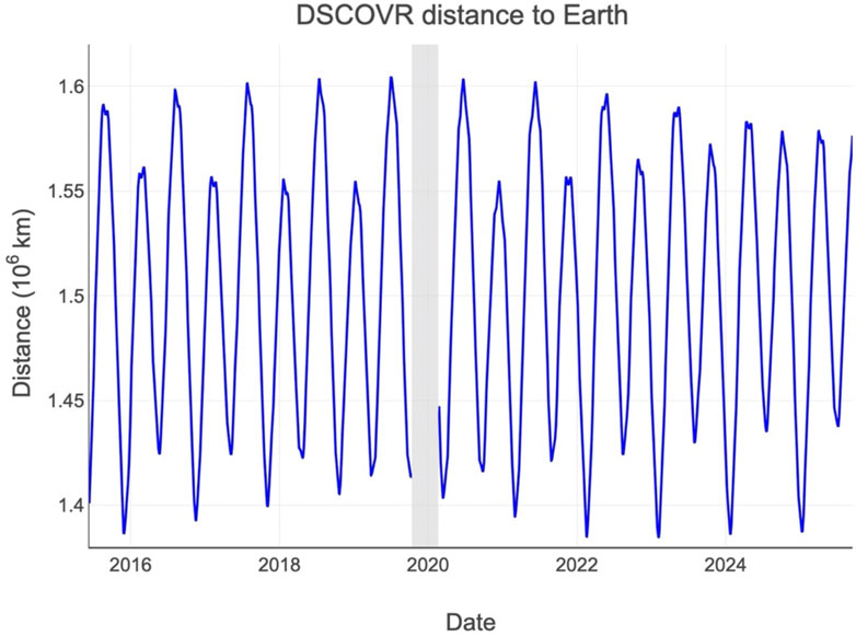
Figure 1. Distance between Earth and DSCOVR (in 106 km). Shadowed area shows the spacecraft’s safe hold period (from 27 June 2019, to 19 February 2020).
To simulate coarser resolutions, we down-sampled each cropped image to eight target sizes (1,024, 512, … , 8 pixels per side, or ∼12, 25, 50, 100, 200, 400, 800, 1,600 km, respectively). We define a “superpixel” as a contiguous N × N block of original image pixels aggregated into one lower-resolution cell. For our reflectance bands, we preserved the dominant spectral features by averaging the valid pixels within each superpixel, retaining that mean value only when more than 50% of its constituent pixels contained valid data. For the cloud fraction binary mask, we implemented five distinct threshold rules that designate a superpixel as “cloudy” if at least one pixel is cloudy, more than 25% of the pixels are cloudy, or ≥50%, ≥75%, or 100% - all the pixels of its constituent high-resolution pixels are cloudy. This allowed us to explore the sensitivity of cloud-fraction estimates to different sub-pixel classification assumptions. We then computed “cloud fraction” as the ratio of cloudy to total valid pixels for each combination of observation, resolution, and threshold rule.
When we resample the Level-2 EPIC cloud-height and optical-thickness fields onto coarser grids, each superpixel was formed by grouping together a block of the original high-resolution pixels. Within each block, we distinguished valid cloud retrievals (pixels with height or thickness values) from clear-sky or background pixels, which are recorded as NaN. We then counted how many subpixels carry valid retrievals: if at least 50% of the block is valid, we computed the superpixel’s value as the arithmetic mean of those retrievals, effectively ignoring the NaNs. For instance, if three of four subpixels report cloud height and one is clear-sky (NaN), the superpixel height is simply the average of the three cloud heights. Conversely, if fewer than half of the subpixels contain valid information (for example, one cloudy pixel and three clear), then the entire superpixel was set to NaN, preventing clear-sky-dominated areas from skewing our aggregated statistics. After calculating the superpixels, we averaged the full disk for each resolution.
3 Results
EPIC acquires all ten spectral bands at a native nadir sampling of approximately 8 km × 8 km, but it performs a 2 × 2 onboard pixel-averaging (binning) for every band except the 443 nm (blue) channel to stay within the spacecraft’s downlink budget. For example, Figure 2 illustrates how a more aggressive down-sampling affects the binary cloud mask of one EPIC image using the 50% threshold rule. This corresponds to a ground sampling distance of: roughly ∼6400 km at 2 × 2 resolution; 3200 km at 4 × 4; 1,600 km at 8 × 8; 800 km at 16 × 16; 400 km at 32 × 32; 200 km at 64 × 64; 100 km at 128 × 128; 50 km at 256 × 256; 25 km at 512 × 512; finally, just 12 km at 1,024 × 1,024. Thus, as we move from the coarsest (2 px) to the finest (1,024 px) grid, the effective pixel size shrinks by more than three orders of magnitude, from continental scales (∼6400 km) down to mesoscale features (12 km).
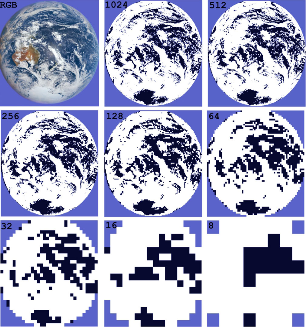
Figure 2. Binary cloud mask heatmap for down-sampled resolutions using the 50% threshold rule from 1,024 px to 8 px. Pixel size is approximately 10 km at native resolution and 1,600 km at 8 px.
3.1 Reflectances
Unlike atmospheric properties (cloudy/clear), top-of-atmosphere reflectance is fundamentally a continuous, smoothly varying field. When studying the implications of spatial scaling, averaging or majority-voting blocks of pixels have very little impact on its global mean. EPIC’s radiometric calibration produces relatively noise-free reflectance maps that vary gradually on scales of tens to hundreds of kilometers. Even in extreme down-sampling from 1,024 × 1,024 down to 8 × 8 pixels (from 12 × 12 km2 to 1600 × 1600 km2), the spatial smoothing inherent in coarse gridding simply blurs fine detail but preserves the overall brightness. Since each superpixel value is ultimately an average of many highly correlated neighbors, the disk-integrated mean reflectance hardly budges.
Figure 3 presents the reflectance time series in multiple spectral bands for selected days in 2020. The daily amplitude (vertical variability) mostly reflects the changing land–ocean composition within each scene, while each wavelength also exhibits its own seasonal cycle. To illustrate the impact of spatial aggregation, we show results at four resolutions: 512 px, 128 px, 32 px, and 8 px.
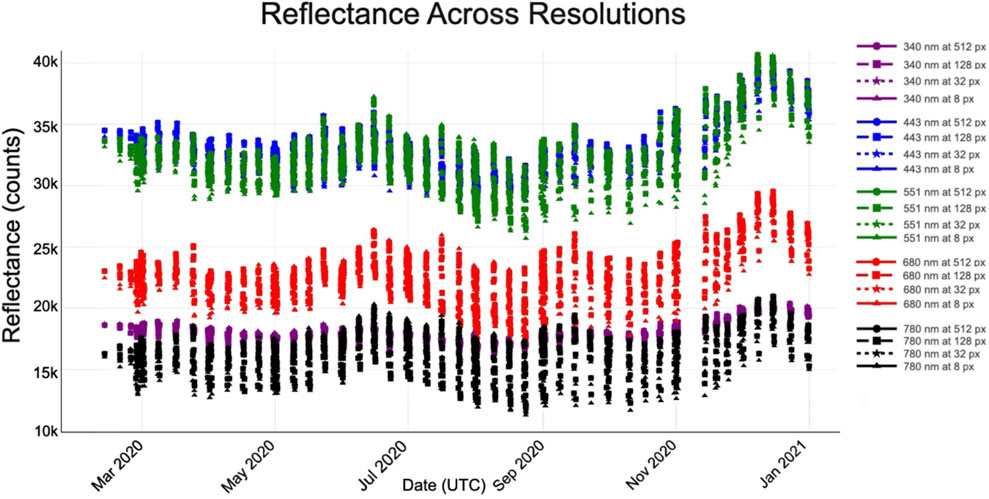
Figure 3. Mean top-of-atmosphere reflectance as a function of spatial resolution for five EPIC spectral bands (340, 443, 551, 680, and 780 nm). Each line shows the aggregated reflectance at super-pixel sizes of 512, 128, 32, and 8 pixels (∼25, 100, 400, and 1,600 km), illustrating how coarsening the grid preserves the spectral signal. The vertical variability within each day is mostly due to the changes in the land/ocean fraction of each image as the Earth rotates.
Figure 4 provides a close-up comparison of the globally integrated reflectances on two summer days. Across every wavelength, the various pixel resolutions yield virtually identical values, with only the 8px line differing by less than 1%. As Earth rotates, EPIC samples change surface characteristics, which in turn alters both the intensity and spectral composition of the reflected radiation field. As seen in the figure, this natural temporal modulation of the radiation measurements is by far more impactful than the resolution effects.
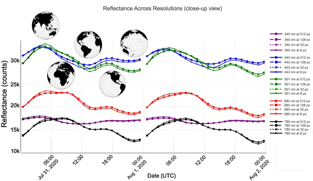
Figure 4. Close-up view of Figure 1 showing the five wavelengths at selected spatial resolutions. Reflectances remain nearly invariant under resolution scaling, with only the coarsest sampling (8 px) exhibiting noticeable deviations from the other resolutions.
Beyond spatial-resolution effects, several geophysical and observational factors introduce substantial variability in EPIC radiances. First, changes in solar zenith angle throughout the day modulate atmospheric path length and scattering geometry, directly altering observed reflectances (Marshak et al., 2021). Second, fluctuations in atmospheric constituents such as aerosols and water vapor can significantly perturb radiance fields. Elevated aerosol loading increases scattering in the UV and visible, while variable precipitable water vapor primarily affects absorption in near-infrared bands (Cede et al., 2025; Yang et al., 2019). Third, clouds are inherently the largest source of radiance variability; their fractional coverage, vertical extent, and optical thickness can alter disk-integrated reflectances by tens of a percent on diurnal timescales (Delgado-Bonal et al., 2020; Delgado-Bonal et al., 2021; Delgado-Bonal et al., 2024). Finally, surface bidirectional reflectance distribution function (BRDF) anisotropy, driven by land-cover type and sun–sensor geometry, introduces additional modulation in the signal, particularly over bright deserts and vegetated regions (Loeb and Coakley, 1998; Oreopoulos and Davies, 1998).
The relative contribution of these factors depends on wavelength, time of day, and scene type. For example, solar zenith effects dominate shortwave variability over the ocean, whereas aerosol and water vapor absorption are more important in polluted or humid regions. Cloud variability generally exceeds surface BRDF effects in magnitude, but the latter can still bias apparent albedo when not properly accounted for. Disentangling these contributions is therefore essential for interpreting radiance time series and for isolating scale-driven biases from true geophysical variability.
3.2 Cloud fraction
Although reflectance changes linearly under spatial aggregation such that the mean of means remains almost unchanged, cloud metrics exhibit pronounced non-linearity because they derive from binary, threshold-based classifications. Higher spatial resolution effectively disentangles mixed clear-sky and cloudy pixels, exposing low-coverage regions that coarse sensors subsume into wholly cloudy pixels. Consequently, while aggregated reflectance curves remain nearly invariant across resolutions, cloud fraction and related cloud property estimates display a strong dependence on pixel size.
Real clouds exhibit sharp edges and small-scale variability: broken cumulus fields, thin cirrus veils, and sub-pixel clear-sky holes. At high resolution, EPIC picks up those clear-sky breaks, so the overall cloud fraction is driven down by the numerous small clear pixels. However, as resolution degrades, each coarse superpixel inevitably contains at least one cloudy measurement, and under any threshold rule that admits partial cloudiness, that superpixel becomes classified as 100% cloudy. Thus, cloud fraction and related metrics (height and optical thickness) climb steeply at coarse resolution, even though the true, sub-pixel cloud fraction has not changed.
Figure 5 shows cloud fraction as a function of spatial resolution and threshold choice, highlighting the profound impact of both pixel size and the aggregation rule on what we call “cloudy.” In our analysis, the “one-pixel” threshold (where any presence of cloud in a superpixel marks it as fully cloudy) produces the highest cloud fractions at all resolutions, reflecting the most permissive criterion. At the finest resolution (1,024 × 1,024), this threshold already yields a cloud fraction well above 0.7, rising to unity as the coarse grid approaches a few pixels across the disk. By contrast, the “100%” threshold (i.e., requiring every sub-pixel to be cloudy) delivers the lowest estimates, demonstrating that only completely overcast superpixels survive at coarse scales. Intermediate thresholds (25%, 50%, and 75%) span this envelope but themselves exhibit strong resolution dependence—at fine resolution, they converge towards similar values (as individual pixels are small and often uniformly cloudy or clear), yet as resolution degrades, the curves diverge, with lower thresholds climbing more steeply toward unity.
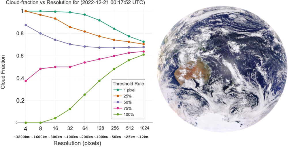
Figure 5. Cloud-fraction values as a function of spatial resolution in log-scale for a single EPIC observation (2022–12-21). Five threshold rules are shown (“1 pixel,” “25%,” “50%,” “75%,” and “100%”) indicating the minimum number or fraction of cloudy sub-pixels required to classify a super-pixel as cloudy. This plot highlights how both grid coarsening and threshold choice jointly affect the estimated cloud fraction. Resolutions of 1,024, 512, 256, 128, 64, 32, 16, and 8 pixels correspond to ∼12, 25, 50, 100, 200, 400, 800, and 1,600 km, respectively.
These patterns mirror classic studies of cloud-fraction sensitivity. As Hobbs and Rangno (1998) and later Jones et al. (2012) have shown, coarse pixels inevitably contain at least some cloudy sub-pixels, so permissive thresholds severely overestimate cover. Meanwhile, the conventional majority-vote rule of a 50% threshold lies between these extremes but still overestimates by tens of a percent at kilometer-scale grids.
Physically, these differences arise because cloud fields are highly heterogeneous on sub-kilometer scales (Davis et al., 1999; Gerber et al., 2001). Broken cumulus and thin cirrus interweave clear sky and cloud, so even a modest aggregation window will almost always include some cloudy footprints. With a 25% rule, only a few cloudy pixels suffice to classify the entire superpixel as cloudy, artificially merging broken fields into nearly overcast scenes. Conversely, the “100%” rule demands truly homogeneous clouds and thus preserves the small clear gaps that coarse mean methods would otherwise smooth over. This tension between aggregation and true sub-pixel variability underlies the plane-parallel biases in optical property retrievals noted, for example, by Loeb and Coakley (1998) and Zhang et al. (2016).
3.3 Cloud height and cloud optical thickness
Figure 6 shows a panel with daily mean cloud-effective height (top row) and cloud optical thickness (bottom row) as functions of spatial resolution, separated into low clouds (tops below 5,000 m whose most likely thermodynamic phase is liquid) and high clouds (tops above 5,000 m whose most likely thermodynamic phase is ice). The results indicate a systematic tendency for both quantities to increase as resolution becomes coarser. For low clouds, degrading the resolution from approximately 12 km to 400 km raises the retrieved mean cloud height by nearly 1 km and produces a marked increase in optical thickness. High clouds exhibit more stability, with mean values remaining closer across most resolutions, but at the coarsest sampling, the distributions display slightly higher scatter and a modest upward shift in optical thickness. Similar resolution-driven biases have been documented when comparing ASTER (15 m), MISR (275 m), and MODIS (1 km) cloud retrievals, underscoring that coarse sampling systematically alters the statistical distribution of cloud properties (Zhao and Di Girolamo, 2007; Marchand et al., 2010; Mitra et al., 2021; Li et al., 2016).
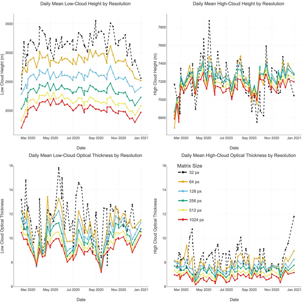
Figure 6. Daily mean cloud-effective height and cloud optical thickness as functions of spatial resolution, shown separately for low (<5 km; left panels) and high clouds (>5 km; right panels). A 50% threshold rule was applied, retaining a coarse pixel only when at least half of its subpixels contained valid retrievals. As spatial resolution degrades from ∼12 km (1,024 px) to ∼400 km (32 px), low clouds exhibit a pronounced resolution dependence: the mean cloud-top height rises by nearly 1 km, and the mean optical thickness increases substantially, indicating that subpixel mixing and preferential sampling bias retrievals toward taller and optically thicker clouds. By contrast, high-cloud heights and optical thicknesses remain comparatively stable across most resolutions, with only the coarsest sampling showing greater variability.
The underlying causes of these biases lie in both sampling effects and nonlinear averaging. Under the 50% thresholding rule used in our analysis, a coarse pixel is retained only if at least half of its subpixels contain valid cloud retrievals. Thin or spatially sparse low clouds often fail this criterion when aggregated and are therefore excluded at coarse resolution. In contrast, larger contiguous regions of thick or tall clouds are more likely to meet the threshold and thus dominate the retained sample. This preferential sampling skews the distribution toward the tallest and most optically dense clouds as resolution degrades (Zhao and Di Girolamo, 2007; Marchand et al., 2010; Mitra et al., 2021).
Nonlinear radiative effects further amplify this shift. When clear, thin, and thick cloud subpixels are averaged together within a coarse pixel, the reflectance–optical thickness relationship is not linear. Because reflectance responds disproportionately to large optical depths, the coarse-pixel mean corresponds to a τ higher than the simple average of its subpixels—a manifestation of the well-known plane-parallel bias (Davis et al., 1997; Zhang et al., 2012; Cornet et al., 2018). A similar radiative weighting occurs for cloud height, where tall cloud elements within a pixel can dominate the signal and pull the effective height upward. Together, preferential sampling and nonlinear averaging explain why both height and optical thickness rise at coarse resolution.
A second, equally important outcome is the increase in variability of the retrieved properties as the resolution decreases. For low clouds, the scatter in both height and optical thickness grows substantially with pixel size, reflecting the fact that coarse pixels blend highly heterogeneous cloud fields in different proportions from scene to scene. In one coarse pixel, a few deep convective towers may drive the retrieval, while in another, more homogeneous stratiform clouds dominate. This mixing produces greater scene-to-scene fluctuations because each coarse retrieval collapses diverse cloud populations into a single value.
To better illustrate the scaling behavior and scene-to-scene variability, Figure 7 shows how cloud effective heights vary with spatial resolution for two EPIC snapshots taken on the same day at different times. The 17 UTC scene (centered on the Americas) and the 11 UTC scene (dominated by Africa) are each plotted with low-cloud heights on the left and high-cloud heights on the right. Superpixel sizes range from 32 to 1,024 px, corresponding roughly from 400 km down to 12 km per pixel along the x-axis, while the y-axis reports the disk averaged height in meters. We observe a clear change in scaling behavior below 64 px (∼200 km), depending on the scene that EPIC observes, for both low and high clouds. These contrasts highlight that retrievals made at spatial scales coarser than roughly 200 km per pixel are prone to significant aggregation artifacts, but we also note that part of the difference between the two cases may reflect underlying variations in meteorological conditions, cloud regimes, and viewing geometry across the Americas and Africa. Thus, the distinct behaviors seen in Figure 7 likely result from an interplay between resolution-driven sampling effects and regional scene characteristics.
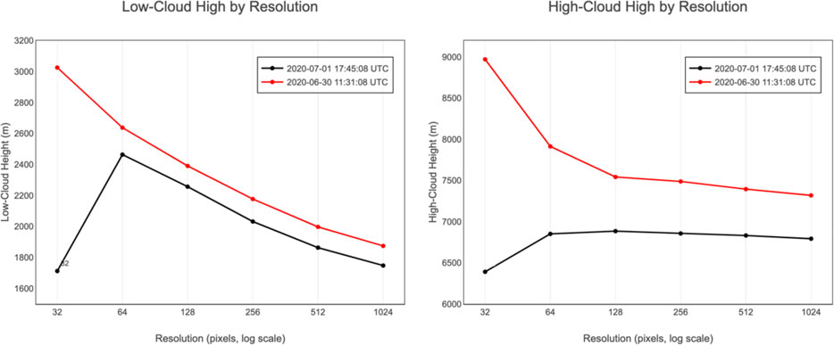
Figure 7. Cloud-effective height for two EPIC images of the same day as a function of spatial resolution with a 50% threshold rule. The EPIC field of view at 17 UTC captures the Americas in the center of the image, while 11 a.m. is dominated by Africa (see Figure 3). Left: low-cloud heights; right: high-cloud heights. The x-axis shows superpixel size (32–1,024 px), and the y-axis gives cloud height in meters. Scaling properties change drastically at 64 pixels (∼200 km per pixel).
4 Conclusion
Our analysis reveals that while global-mean top-of-atmosphere reflectance remains essentially invariant (±1%) when down-sampled from 1,024 × 1,024 to 8 × 8 pixels—owing to the smoothly varying nature of reflectance fields—retrieved cloud properties exhibit pronounced, resolution-dependent biases. As spatial resolution coarsens, cloud fraction changes sharply depending on the selected threshold rule. Our multi-threshold curves quantify how the choice of threshold, and thus the assumed homogeneity of a superpixel, influence cloud fraction with resolution. For applications ranging from climate model evaluation to exoplanet analog studies, these findings underscore that both spatial scale and classification rule must be reported. Ultimately, high-resolution observations (tens of meters) remain essential to benchmark and correct the biases inherent in kilometer-scale cloud products.
When we set a 50% threshold for cloud-effective height and optical thickness, the mean values increased as resolution coarsened: coarser grids preferentially retain taller, thicker cloud features while discarding thin or invalid subpixels (ignoring small clouds), skewing the global averages upward by several hundred meters in height and tens of percent in optical thickness.
Biases in coarse-resolution cloud fields can substantially distort estimates of Earth’s energy balance and cloud radiative forcing. Low-level liquid clouds primarily cool the planet by reflecting incoming solar radiation (negative shortwave forcing) but also contribute a lesser greenhouse warming by trapping outgoing longwave radiation. Overestimating cloud-top height enhances the layer’s longwave emissivity, thereby exaggerating the amount of outgoing longwave radiation that is trapped. Overestimating cloud optical thickness directly leads to inflated albedo values, which in turn exaggerates the magnitude of shortwave cooling. As a result, top-of-atmosphere radiative fluxes derived from coarse-resolution products will be biased toward both stronger cooling and stronger warming effects than reality. Similarly, overestimating the height and thickness of high-altitude cirrus amplifies their positive longwave forcing, further skewing modeled radiative balances.
Data availability statement
The original contributions presented in the study are included in the article/supplementary material; further inquiries can be directed to the corresponding author.
Author contributions
AD-B: Conceptualization, Writing – review and editing, Writing – original draft, Formal Analysis, Investigation. AM: Methodology, Visualization, Conceptualization, Writing – review and editing, Supervision. YY: Conceptualization, Writing – review and editing, Supervision, Methodology.
Funding
The author(s) declare that financial support was received for the research and/or publication of this article. AD-B is supported by the DSCOVR Science Management project and the DSCOVR Science Team Program. AM acknowledges funding support from the DSCOVR Science Management project. YY acknowledges funding support from the NASA DSCOVR Science Team Program.
Conflict of interest
The authors declare that the research was conducted in the absence of any commercial or financial relationships that could be construed as a potential conflict of interest.
The author(s) declared that they were an editorial board member of Frontiers at the time of submission. This had no impact on the peer review process and the final decision.
Generative AI statement
The author(s) declare that no Generative AI was used in the creation of this manuscript.
Any alternative text (alt text) provided alongside figures in this article has been generated by Frontiers with the support of artificial intelligence and reasonable efforts have been made to ensure accuracy, including review by the authors wherever possible. If you identify any issues, please contact us.
Publisher’s note
All claims expressed in this article are solely those of the authors and do not necessarily represent those of their affiliated organizations, or those of the publisher, the editors and the reviewers. Any product that may be evaluated in this article, or claim that may be made by its manufacturer, is not guaranteed or endorsed by the publisher.
References
Cahalan, R. F., Ridgway, W., Wiscombe, W. J., Bell, T. L., and Snider, J. B. (1994). The albedo of fractal stratocumulus clouds. J. Atmos. Sci. 51, 2434–2455. doi:10.1175/1520-0469(1994)051<2434:taofsc>2.0.co;2
Cede, A., Rajagopalan, R., Yu, Y., Marshak, A., Herman, J., Huang, L. K., et al. (2025). EPIC and NISTAR radiometric stability assessment using ERA5 reanalysis data. Front. Remote Sens 6, 1646764. doi:10.3389/frsen.2025.1646764
Cornet, C., C.-Labonnote, L., Waquet, F., Szczap, F., Deaconu, L., Parol, F., et al. (2018). Cloud heterogeneity on cloud and aerosol above cloud properties retrieved from simulated total and polarized reflectances. Atmos. Meas. Tech. 11, 3627–3643. doi:10.5194/amt-11-3627-2018
Cowan, N. B., Agol, E., Meadows, V. S., Robinson, T., Livengood, T. A., Deming, D., et al. (2009). Alien maps of an ocean-bearing world. Astrophysical J. 700* (2), 915–923. doi:10.1088/0004-637X/700/2/915
Davis, A., Marshak, A., Cahalan, R., and Wiscombe, W. (1997). The landsat scale-break in stratocumulus as a three-dimensional radiative transfer effect, implications for cloud remote sensing. J. Atmos. Sci. 54, 241–260. doi:10.1175/1520-0469(1997)054<0241:tlsbis>2.0.co;2
Davis, A., Marshak, A., Gerber, H., and Wiscombe, W. (1999). Horizontal structure of marine boundary layer clouds from centimeter to kilometer scales. J. Geophys. Res. 104, 6123–6144. doi:10.1029/1998jd200078
De Vera, M. V., Di Girolamo, L., Zhao, G., Rauber, R. M., Nesbitt, S. W., and McFarquhar, G. M. (2024). Observations of the macrophysical properties of cumulus cloud fields over the tropical western Pacific and their connection to meteorological variables. Atmos. Chem. Phys. 24 (9), 5603–5623. doi:10.5194/acp-24-5603-2024
Delgado-Bonal, A., Marshak, A., Yang, Y., and Oreopoulos, L. (2020). Daytime variability of cloud fraction from DSCOVR/EPIC observations. J. Geophys. Res. 125 (10), e2019JD031488. doi:10.1029/2019JD031488
Delgado-Bonal, A., Marshak, A., Yang, Y., and Oreopoulos, L. (2021). Global daytime variability of clouds from DSCOVR/EPIC observations. Geophys. Res. Lett. 48, e2020GL091511. doi:10.1029/2020GL091511
Delgado-Bonal, A., Marshak, A., Yang, Y., and Oreopoulos, L. (2022). Cloud height daytime variability from DSCOVR/EPIC and GOES-R/ABI observations. Front. Remote Sens. 3, 780243. doi:10.3389/frsen.2022.780243
Delgado-Bonal, A., Marshak, A., Yang, Y., and Oreopoulos, L. (2024). Global cloud optical depth daily variability based on DSCOVR/EPIC observations. Front. Remote Sens. 5, 1390683. doi:10.3389/frsen.2024.1390683
Di Girolamo, L., Liang, L., and Platnick, S. (2010). A global view of one-dimensional solar radiative transfer through oceanic water clouds. Geophys. Res. Lett. 37, L18809. doi:10.1029/2010GL044094
Gerber, H., Jensen, J., Davis, A., Marshak, A., and Wiscombe, W. (2001). Spectral density of cloud liquid water content at high frequencies. J. Atmos. Sci. 58, 497–503. doi:10.1175/1520-0469(2001)058<0497:sdoclw>2.0.co;2
Hobbs, P. V., and Rangno, A. L. (1998). Microstructures of low and middle-level clouds over the beaufort sea. Q. J. R. Meteorol. Soc. 124, 2035–2071. doi:10.1002/qj.49712455012
Jiang, J. H., Li, J. L., Olsen, K., Zhai, C., Yung, Y. L., Crisp, D., et al. (2018). Using deep space climate observatory measurements to study the Earth as an exoplanet. Astronomical J. 156 (1), 26. doi:10.3847/1538-3881/aac6e2
Jones, A. L., Di Girolamo, L., and Zhao, G. (2012). Reducing the resolution bias in cloud fraction from satellite derived clear-conservative cloud masks. J. Geophys. Res. 117, D12201. doi:10.1029/2011JD017195
Li, J. L., Zhang, Z., and Di Girolamo, L. (2016). A framework based on 2-D taylor expansion for quantifying the impacts of subpixel reflectance variance and covariance on cloud optical thickness and effective radius retrievals based on the bispectral method. J. Geophys. Res. Atmos. 121 (17), 10,233–10,248.
Loeb, N. G., and Coakley, J. A. (1998). Inference of marine stratus cloud optical depths from satellite measurements: does 1D theory apply? J. Clim. 11, 215–233. doi:10.1175/1520-0442(1998)011<0215:IOMSCO>2.0.CO;2
Loeb, N. G., Varnai, T., and Winker, D. M. (1998). Influence of subpixel scale cloud top structure on reflectances from overcast stratiform cloud layers. J. Atmos. Sci. 55 (19), 2960–2973. doi:10.1175/1520-0469(1998)055<2960:IOSSCT>2.0.CO;2
Marchand, R., Ackerman, T., Smyth, M., and Rossow, W. B. (2010). A review of cloud top height and optical depth histograms from MISR, ISCCP, and MODIS. J. Geophys. Res. 115, D16206. doi:10.1029/2009JD013422
Marshak, A., Davis, A., Wiscombe, W., and Cahalan, R. (1995). Radiative smoothing in fractal clouds. J. Geophys. Res. 100 (D12), 26247–26261. doi:10.1029/95JD02895
Marshak, A., Platnick, S. E., Varnai, T., Wen, G., and Cahalan, R. F. (2006). Impact of three-dimensional radiative effects on satellite retrievals of cloud droplet sizes. J. Geophys. Res. 111 (D9), D09207. doi:10.1029/2005JD006686
Marshak, A., Herman, J., Szabo, A., Blank, K., Cede, A., Carn, S., et al. (2018). Earth observations from DSCOVR/EPIC instrument. Bull. Amer. Meteor. Soc. (BAMS) 9, 1829–1850. doi:10.1175/BAMS-D-17-0223.1
Marshak, A., Delgado-Bonal, A., and Knyazikhin, Y. (2021). Effect of scattering angle on Earth reflectance. Front. Remote Sens. 2, 719610. doi:10.3389/frsen.2021.719610
Mitra, A., Di Girolamo, L., Hong, Y., Zhan, Y., and Mueller, K. J. (2021). Assessment and error analysis of Terra-MODIS and MISR cloud-top heights through comparison with ISS-CATS lidar. J. Geophys. Res. Atmos., 126. doi:10.1029/2020JD034281
Oreopoulos, L., and Cahalan, R. F. (2005). Cloud inhomogeneity from MODIS. J. Clim. 18, 5110–5124. doi:10.1175/JCLI3591.1
Oreopoulos, L., and Davies, R. (1998). Plane parallel albedo biases from satellite observations. Part I: dependence on resolution and other factors. J. Clim. 11 (4), 919–932. doi:10.1175/1520-0442(1998)011<0919:PPABFS>2.0.CO;2
Pierrehumbert, R. T. (1996). Anomalous scaling of high cloud variability in the tropical Pacific. Geophys. Res. Lett. 23 (8), 1095–1098. doi:10.1029/96GL01121
Robinson, T. D., Meadows, V. S., Crisp, D., Deming, D., A'Hearn, M. F., Charbonneau, D., et al. (2011). Earth as an extrasolar planet: earth model validation using EPOXI Earth observations. Astrobiology 11 (5), 393–408. doi:10.1089/ast.2011.0642
Shenk, W. E., and Salomonson, V. V. (1972). A simulation study exploring the effects of sensor spatial resolution on estimates of cloud cover from satellites. J. Appl. Meteor. Climatol. 11, 214–220. doi:10.1175/1520-0450(1972)011<0214:ASSETE>2.0.CO;2
Wen, G., Marshak, A., Su, W., and Weatherhead, E. (2025). Hourly, daily, and monthly variabilities of spectral reflectance and shortwave flux from EPIC observations. Front. Remote Sens. 6, 1657038. doi:10.3389/frsen.2025.1657038
Yang, Y., Meyer, K., Wind, G., Zhou, Y., Marshak, A., Platnick, S., et al. (2019). Cloud products from the earth polychromatic imaging camera (EPIC): algorithms and initial evaluation. Atmos. Meas. Tech. 12, 2019–2031. doi:10.5194/amt-12-2019-2019
Yang, Y., Bhatta, S., and Delgado-Bonal, A. (2025). Decadal observations of global daytime cloud properties from DSCOVR–EPIC. Front. Remote Sens. 6, 1632157. doi:10.3389/frsen.2025.1632157
Zhang, Z., Ackerman, A. S., Feingold, G., Platnick, S., Pincus, R., and Xue, H. (2012). Effects of cloud horizontal inhomogeneity and drizzle on remote sensing of cloud droplet effective radius: case studies based on large-eddy simulations. J. Geophys. Res. Atmos. 117 (D19). doi:10.1029/2012JD017655
Zhang, Z., Werner, F., Cho, H., Wind, G., Platnick, S., Ackerman, A. S., et al. (2016). A framework based on 2-D taylor expansion for quantifying the impacts of subpixel reflectance variance and covariance on cloud optical thickness and effective radius retrievals based on the bispectral method. J. Geophys. Res. 121, 7007–7025. doi:10.1002/2016JD024837
Keywords: spatial resolution, cloud fraction, plane-parallel biases, cloud optical thickness, droplet effective radius, earth observation instruments, exoplanet observations, disk-integrated data
Citation: Delgado-Bonal A, Marshak A and Yang Y (2025) Size matters: the influence of pixel resolution on DSCOVR/EPIC reflectance and cloud metrics. Front. Remote Sens. 6:1683919. doi: 10.3389/frsen.2025.1683919
Received: 11 August 2025; Accepted: 13 October 2025;
Published: 12 November 2025.
Edited by:
Sawaid Abbas, University of the Punjab, PakistanReviewed by:
Dongchen Li, Texas A and M University, United StatesHong Chen, University of Colorado Boulder, United States
Copyright © 2025 Delgado-Bonal, Marshak and Yang. This is an open-access article distributed under the terms of the Creative Commons Attribution License (CC BY). The use, distribution or reproduction in other forums is permitted, provided the original author(s) and the copyright owner(s) are credited and that the original publication in this journal is cited, in accordance with accepted academic practice. No use, distribution or reproduction is permitted which does not comply with these terms.
*Correspondence: Alfonso Delgado-Bonal, YWxmb25zby5kZWxnYWRvYm9uYWxAbmFzYS5nb3Y=