Application of radon transform to multi-angle measurements made by the research scanning polarimeter: a new approach to cloud tomography. Part II: examples of retrievals from CAMP2Ex dataset

In Part II of the series we present results of application of our recently developed tomographic technique to real measurements made by the Research Scanning Polarimeter (RSP). This instrument served as a prototype for the Aerosol Polarimetery Sensor launched on-board the NASA Glory satellite. The retrieval algorithms developed for the Research Scanning Polarimeter were adopted for analysis of the measurements by the space-borne polarimeters on the recently launched NASA's Plankton, Aerosol, Cloud Ocean Ecosystem (PACE) satellite. The RSP is an airborne along-track scanner with uniquely high angular resolution and high frequency of measurements. Besides characterization of liquid-water cloud droplet sizes the RSP observations also provide for derivation of 2D fields of extinction coefficient inside the cloud using a tomographic technique described in Part I of the series. This technique utilizes the family of cloud shapes derived using “cutout” method, which can be interpreted as level curves of an abstract “reflectance density”. The latter is then used for derivation of the directional cloud optical thickness (dCOT) tomogram, a collection of dCOTs is parameterized by the angles and offsets of the view rays (chords). After this, the inverse Radon Transform (the mathematical basis of the X-ray computed tomography) is applied to the dCOT tomogram yielding 2D spatial distribution of the extinction coefficient. The later can be converted into droplet number concentration using the droplet size profiles derived from the RSP’s polarized reflectance measurements. After successful tests on synthetic data, this technique was applied to real RSP measurements from NASA’s Cloud, Aerosol and Monsoon Processes Philippines Experiment (${\text{CAMP}}^2$Ex) conducted in the vicinity of the Philippines during the Southwest Monsoon (August–September 2019). We have investigated the interiors of a number of clouds observed during ${\text{CAMP}}^2$Ex focusing on Cu and CuCg (Tcu) cases, two of which are presented in this paper. Our retrievals were compared with the correlative measurements by lidar (HSRL-2) and cloud radar (APR-3) that were deployed on the same airborne platform (NASA’s P-3B) during this field experiment.

1 Introduction

Cloud tomography is a common name for a number of remote sensing techniques aiming to estimate the structure of cloud interior from optical measurements made outside the cloud. The typical outputs of such algorithms are 2D or 3D fields of droplet extinction coefficients and number concentrations. Such information is usually provided by in situ measurements made inside cloud. Tomographic retrievals, while being less accurate, can complement localized in situ measurements (when available) by yielding the instant microphysical structure of the cloud as a whole.

The cloud tomography algorithm used in this study was introduced by Alexandrov et al. (2021) hereinafter referred to as Part I. In this study we demonstrate the performance of this algorithm on real measurements made by the Research Scanning Polarimeter (RSP).

Tomography (from Greek word $\tau o\mu o\varsigma$, tomos, meaning “slice”) is a retrieval technique inverting 2D spatial density from a dataset of integrals of this density taken over a number of transect lines (chords). Each of these integrals is derived from the measured attenuation of a ray sent through the object and captured by detector on the other side. The collection of such integrals parameterized by angles and offsets of these rays constitutes a 2D dataset called “tomogram”. The 2D density can be restored back from its tomogram using the inverse Radon transform, introduced in 1917 by Austrian mathematician Johann Radon (Radon, 1917; Radon and Parks, 1986). This transform serves as the mathematical basis for X-ray computed tomography commonly known as CT scan in medicine. While the term “tomography” in a strict sense is related to essentially active measurements, it is commonly used in cloud remote sensing to describe any technique for estimation of cloud interior structure basing on passive remote optical measurements. Several such techniques currently being developed (e.g., Martin and Hasekamp, 2018; Levis et al., 2020; Doicu et al., 2022a; Doicu et al., 2022b; Tzabari et al., 2022; Loveridge et al., 2023) are based on least-square-fit (LSF) optimization in a multi-dimensional space of 3D cloud configurations. In this approach extensive 3D RT computations need to be performed on each iterative optimization step.

In Part I of this series we presented a new algorithm for inversion of the internal cloud structure which, while relying on passive optical measurements, is closer to the original tomography as it is based on Radon transform rather than LSF techniques. Passive measurements cannot be used directly for the construction of a proper tomogram, defined as the directional cloud optical thickness (dCOT) as a function of angle and offset of the viewing ray. However, such measurements allow for estimation of the tomogram using a certain heuristic approach that does not require 3D RT computations. This approach utilizes the family of cloud shapes derived using “cutout” technique (Alexandrov et al., 2016a) and corresponding to a number of thresholds in measured total reflectance used to separate bright cloud from its darker background. These shapes can be interpreted as level curves of an abstract “reflectance density”, which is then used for deriving the dCOT tomogram based on a proxy formula relating reflectance to dCOT. Once the tomogram is constructed, inverse Radon transform is applied to it yielding a 2D field of the extinction coefficient. This extinction field is defined up to an unknown constant factor and, thus, requires calibration using independent measurements.

The described tomographic retrieval algorithm was designed for application to the Research Scanning Polarimeter measurements, while it can be adapted to data from other similar sensors. The RSP (Cairns et al., 1999) is an airborne high-resolution along-track scanner which provides a sufficient number of view rays at relevant spatial resolution to constrain cloud shapes (Alexandrov et al., 2016a). Other RSP retrieval products are described in the next section.

The new tomographic technique was refined and validated in Part I using a synthetic dataset composed of simulated RSP measurements generated by the 3D radiative transfer (RT) model called “Monte Carlo code for the phYSically correct Tracing of photons In Cloudy atmospheres” (MYSTIC (Mayer, 2009; Emde et al., 2010)). This model was applied to a LES dataset with 100-m horizontal and 40-m vertical resolution representing a shallow maritime convection cloud field. The tomographic retrievals of the extinction coefficient from this dataset appeared to be unbiased in value while having the standard deviation of the difference with the LES values ${\sigma }_k=0.01$ ${\text{m}}^{-1}$ (13.7% of the LES dataset’s maximum). Note that 98% of the retrieved values of $k_{\text{ext}}$ laid within $2{\sigma }_k=0.02$ ${\text{m}}^{-1}$ from their LES counterparts. The extinction coefficient values were then converted into these of cloud droplet number concentration $N_c$ using the profiles of effective radius $(r_{\text{eff}})$ and variance $(v_{\text{eff}})$ of the droplet size distributions (DSDs) derived from the simulated RSP’s polarized reflectance measurements made along the cloud’s side. The comparison of the $N_c$ retrievals with the corresponding LES values showed the standard deviation of the difference ${\sigma }_n=12.3$ ${\text{cm}}^{-3}$ (17% of the maximal $N_c$), while 95.3% of the points in the scatter plot lay within the $2{\sigma }_n$-corridor. The correlation between the RSP and LES $N_c$ values was 80%.

In this paper we present the results of application of our tomographic retrieval algorithm to real RSP measurements made during NASA’s Cloud, Aerosol and Monsoon Processes Philippines Experiment (${\text{CAMP}}^2$Ex) (Reid et al., 2023) conducted in the vicinity of the Philippines in August–September 2019. This field campaign took place during the Southeast Monsoon season, which is characterized by abundance of moisture and strong convections producing wide variety of cloud types and shapes.

2 The RSP measurements and retrievals

The RSP served as a prototype for the satellite Aerosol Polarimetery Sensor (APS) built for the NASA Glory Project (Mishchenko, 2006; Mishchenko et al., 2007). The cloud retrieval algorithms developed for the RSP were recently adopted for use with the measurements of the spaceborne polarimeters on the Plankton, Aerosol, Cloud Ocean Ecosystem (PACE) satellite mission (Werdell and Coauthors, 2019). During the past decades the RSP has been deployed during numerous NASA field campaigns (see, e.g., Alexandrov et al., 2015; Alexandrov et al.,2016a; Alexandrov et al.,2016b; Sinclair et al., 2017; Alexandrov et al., 2018; Sinclair et al., 2019).

The field of view of the RSP is 14 mrad while measurements are made along track at 0.8$°$ intervals within $\pm 60°$ from nadir. This corresponds to the spatial resolution of about 200 m for high-altitude NASA ER-2 aircraft and to less than 100 m for slower NASA airplanes (P-3B, B-200, UC-12, C-130) which fly at lower altitudes (Alexandrov et al., 2016a).

The RSP’s measurements of total and polarized reflectances in 9 spectral channels are used for a number of different kinds of retrievals. The corresponding measurement geometries and the view-line aggregation schemes are presented in Figure 1. The RSP’s polarized reflectance measurements in the rainbow (cloud bow) scattering range (135$°$–165$°$) are being routinely used for retrieval of droplet size distributions in liquid-water clouds (Alexandrov et al., 2012a; b, 2020).

Figure 1

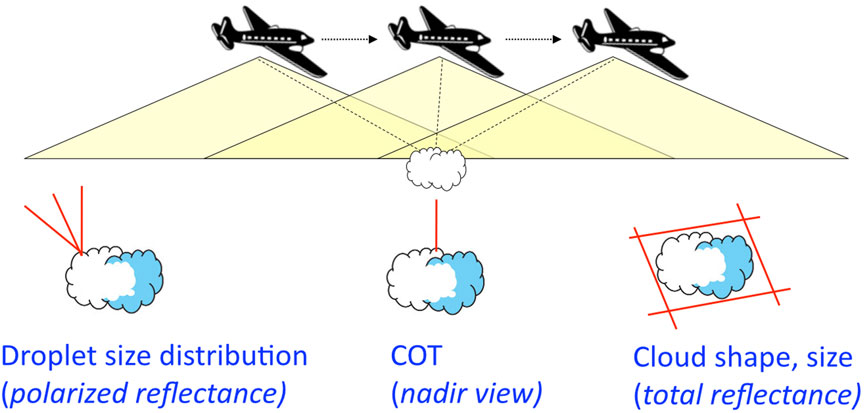
Figure 1. Schematic representation of the RSP’s measurement geometry (top) and the view-line aggregations used for different types of retrievals (bottom). This figure is reproduced from Part I.

The operational algorithm for retrieval of COT from RSP-measured total reflectances at nadir view is a modification of the legacy bi-spectral technique (Nakajima and King, 1990). In the RSP algorithm no absorbing spectral channels are used, while the droplet effective radius is retrieved from the polarized reflectance (Alexandrov et al., 2012a). It is then used to derive the COT value from the look-up table (LUT) computed for non-absorbing 863-nm channel. This LUT is based on plain-parallel radiative transfer computations, thus, the retrieved COT can be biased low in the presence of 3D radiative effects (such as light escape from broken cloud’s sides or shadowing at low sun angles). A correction technique for such biases has been recently suggested by Alexandrov et al. (2024) and Alexandrov et al. (2025). In addition to this, the cloud top heights (CTH) are derived from the RSP data using a stereo block-correlation algorithm (Sinclair et al., 2017).

3 Radon transform

In Part I and in this study we use the implementation of Radon transform from the standard Interactive Data Language (IDL v.8.4) library (RADON function) with the ramp filter added. The geometric setup of the method is schematically shown in Figure 2 (left), while more detailed description can be found in Part I. The 2D field to be determined is the spatial distribution of the cloud extinction coefficient $k_{\text{ext}}(x,y)$ (measured in ${\text{m}}^{-1}$). Its integral over a linear transect (chord) through the cloud (characterized by the angle $\psi$ and the offset $\rho$) yields the directional COT (dCOT). The resulting value of dCOT is attributed to a point with the coordinates $(\psi ,\rho )$ in the Radon space, as shown in Figure 2 (right), and enters the tomogram ${\tau }_{\text{d}}(\psi ,\rho )$. The inverse Radon transform providing the extinction coefficient distribution derived from the tomogram is called “filtered backprojection”. This procedure has two steps: first, the ramp filter is applied to ${\tau }_{\text{d}}(\psi ,\rho )$ in $\rho$-direction, then the backprojection itself is applied to the result yielding the inverted extinction field $k_{\text{ext}}^{\prime }(x,y)$. The inverse Radon transform is not exact, meaning that $k_{\text{ext}}^{\prime }(x,y)$ may slightly differ from the original $k_{\text{ext}}(x,y)$ in spatial structure. The inverted density is also defined up to an unknown constant factor, which must be determined using a calibration procedure based on an independent data source.

Figure 2

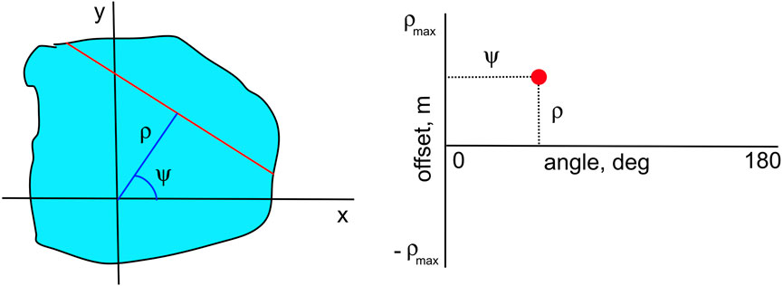
Figure 2. Radon transform geometry: Left: in the physical space the extinction coefficient (light blue) is integrated along the chord (red) parameterized by the angle $\psi$ and the offset $\rho$ in order to get the directional COT ${\tau }_{\text{d}}(\psi ,\rho )$; Right: the representation (red dot) of the location where this chord’s value ${\tau }_{\text{d}}(\psi ,\rho )$ is placed in the Radon’s tomogram. This plot is reproduced from Part I.

In Part I we tested the performance of the IDL RADON function by applying it to a synthetic distribution $k_{\text{ext}}(x,y)$ to compute the tomogram, and then inverting $k_{\text{ext}}^{\prime }(x,y)$ from this tomogram. Calibration was made by matching COT computed from $k_{\text{ext}}^{\prime }(x,y)$ to this from $k_{\text{ext}}(x,y)$. The inverted field appeared to be almost identical to the initial extinction distribution, so the test was successful.

4 Examples from CAMP²Ex dataset

The NASA Cloud, Aerosol and Monsoon Processes Philippines Experiment (${\text{CAMP}}^2$Ex) (Reid et al., 2023) was conducted from Clark International Airport in the Philippines from August 25 to 5 October 2019. Its goal was to improve understanding of interacting aerosol, cloud, and radiation processes within southeast monsoon system. The observations during the campaign were focused on liquid-water and mixed-phase clouds, such as fair weather cumulus (Cu), cumulus congestus (CuCg, also called towering cumulus, Tcu), and altocumulus. Attention was paid to organization of cloud systems and their evolution towards deeper convections. The RSP was deployed on board NASA's P-3B aircraft together with a broad range of other remote sensing and in situ sampling instruments. In this study we are particularly interested in the correlative measurements made by the High Spectral Resolution Lidar (HSRL-2) and the Airborne Third Generation Precipitation Radar (APR-3), which also provides cloud retrievals from its W-band. We will show comparisons of our tomographic retrievals with the data from these two instruments later in the paper. Besides the P-3B payload, measurements were made during this field experiment by instruments on board Stratton Park Engineering Company's (SPEC) Learjet 35 aircraft and at a Manila Observatory ground site.

We will demonstrate performance of our tomographic algorithm on two examples from ${\text{CAMP}}^2$Ex involving different cloud types: Cu cloud observed on 25 August 2019 between 04:23 and 04:24 UTC and CuCg (Tcu) cloud observed on 9 September 2019 between 01:42 and 01:43 UTC. Below we will identify these clouds as Cloud 1 and Cloud 2 respectively. We will apply the tomographic inversion procedure to these clouds step-by-step focusing on cloud-type related differences between these two cases. The corresponding COT time series derived from the RSP data are presented in Figure 3. It is seen from these plots that Cloud 2 is almost three times optically thicker than Cloud 1 (COT of 60 vs. 20 at the maxima).

Figure 3

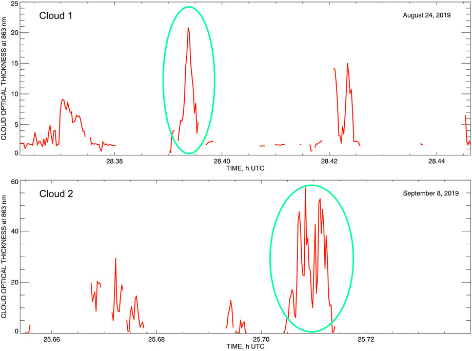
Figure 3. The COT time series derived from the RSP measurements. The two clouds used as examples in this study are singled out by green ellipses. Top: Cu cloud observed on 25 August 2019 between 04:23 and 04:24 UTC. Bottom: CuCg (Tcu) cloud observed on 9 September 2019 between 01:42 and 01:43 UTC. Note that the data in these plots are conventionally labeled by the dates of the flights’ departures (August 24 and September 8 respectively), thus, making the time stamps to run well over 24 h.

4.1 Cloud shapes

We use the “cutout” technique introduced by Alexandrov et al. (2016a) to derive 2D cloud shapes from the RSP measurements (an alternative name used for similar techniques in literature is “space carving” (e.g., Lee et al., 2018; Levis et al., 2020)). This technique uses 1D angular cloud masks constructed for each RSP scan. Choosing a cloud/clear-separation threshold $R_{\text{thr}}$ in the measured total reflectance $R$ allows for distinguishing between the bright $(R>R_{\text{thr}})$ cloudy part of the scan from the darker $(R<R_{\text{thr}})$ background part dominated by the ground surface. If the position of the aircraft in space is accurately known, the viewing angles corresponding to the edges of such cloud mask can be used to construct the two view lines “tangent” to the cloud shape in the vertical plane containing the flight path. This is illustrated by plots in Figure 4 where red and blue lines correspond to different edges of the 1D cloud masks. The collection of all such tangent lines obtained during the cloud overflight effectively “cuts out” a polygon (shown in green) containing the cloud cross-section. Then a disc-inscription technique is used to create a realistically-looking cloud shape (shown in blue) within this polygon (see Alexandrov et al. (2016a) and Part I for details).

Figure 4

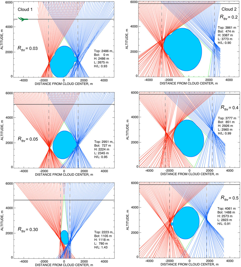
Figure 4. Derivation of the cloud shapes corresponding to various reflectance thresholds $R_{\text{thr}}$. The RSP view rays (red and blue corresponding to different edges of cloud masks) tangent to cloud “surfaces” are used for cutting out polygons (green) in 2D space which are then filled with realistic cloud-shape curves (light blue). Vertical dashed black lines correspond to cloud edges in nadir view. Horisontal black lines show the average aircraft altitudes during the cloud overpasses. Left: Cu case from August 25; Right: CuCg case from September 9.

Cloud shapes derived in such manner are not as universal as those of solid objects: they depend on the brightness thresholds $R_{\text{thr}}$ used for their construction. Higher values of $R_{\text{thr}}$ correspond to smaller cloud cutouts. Also, the optically derived cloud shapes tend to be shifted relative the corresponding physical droplet densities towards the bright side of the cloud.

Figure 4 presents the cloud shapes (and view lines used for their construction) for Cloud 1 (left) and Cloud 2 (right). Plots in each column represent three different reflectance thresholds. Note that the ranges of these thresholds used for the two clouds are quite different: 0.03, 0.05, and 0.3 for Cloud 1 and 0.2, 0.4, and 0.5 for Cloud 2, which appears to be substantially brighter.

Figure 5 (top) shows families of cloud shapes corresponding to a number of $R_{\text{thr}}$ values constructed for our two clouds. While theoretically these families are expected to be nested, in the case of real data it is not always the case because of view-ray construction uncertainties and also some ambiguities in inscribing smooth shapes into the cutout polygons. As the result, some of the shape curves corresponding to different $R_{\text{thr}}$ may be very close to each other at some places or even intersect. However, both families still look close to being nested with the curves corresponding to higher $R_{\text{thr}}$ located “mostly” inside those corresponding to smaller threshold values. The remaining irregularities are taken care of by the algorithm described below.

Figure 5

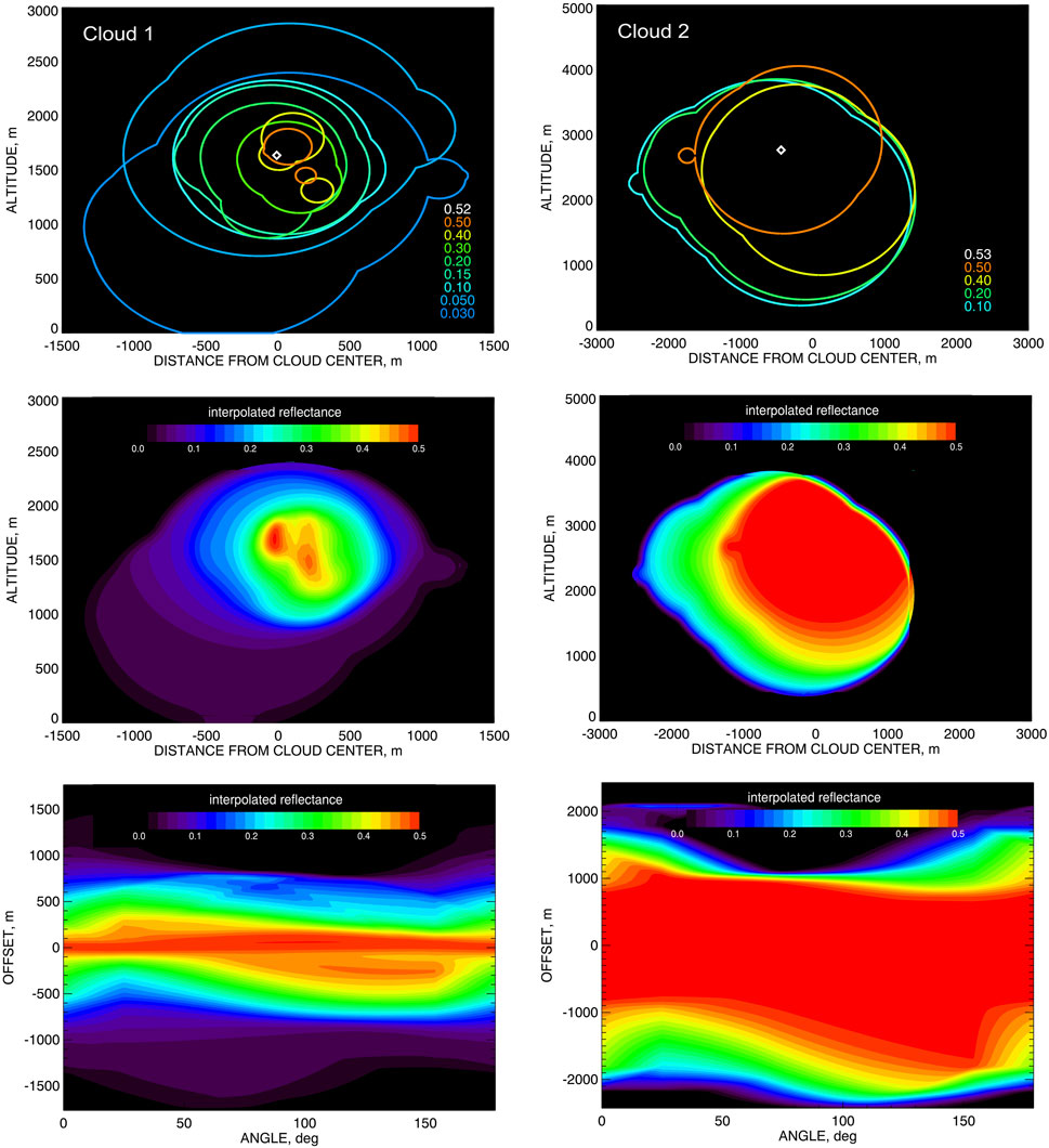
Figure 5. Top: The nested families of cloud shapes corresponding to a number of different reflectance thresholds, the maximal observed reflectance values are assigned to the point at the cloud’s center (depicted by white diamond). Middle: The abstract reflectance-proxy distributions (RPD) computed by interpolation between the curves in the top plots assuming that each point of each curve is assigned the value equal to the corresponding brightness threshold $R_{\text{thr}}$. Bottom: The reflectance tomograms computed for the RPs from middle plots by taking the maxima along the chords. Left: Cloud 1 case from August 25; Right: Cloud 2 case from September 9.

4.2 Reflectance-proxy distribution and its tomogram

The reflectance values $R=R_{\text{thr}}$ are observed only in the directions of the view rays tangent to the corresponding cloud shapes, as it is seen in Figure 4. We extend the notion of reflectance assuming that the value of $R_{\text{thr}}$ can be assigned to all points of the shape curve regardless whether or not there are actual view rays passing through them. Note that for some points near cloud top and bottom such view rays, if existed, would be close to horizontal, which is inconsistent with the RSP’s measurement geometry. Assigning the $R_{\text{thr}}$ values to the points in the shape curves rather than to the view rays allows us to consider the cloud shapes in Figure 5 (top) as level curves of an abstract function in 2D domain occupied by the cloud. We call this function the “reflectance-proxy” (RP) distribution or RPD.

The RP values at the points belonging to the curves in Figure 5 (top) are then interpolated to points in-between the curves, thus, creating the full RPD in the 2D domain bounded by the shape curve with the lowest $R_{\text{thr}}$. For each point $P$ in this domain we first select the two level curves between which it is located. Then, we assign the weights for the RP values of the two curves basing on the shortest distances from $P$ to these curves. These weights are then used to compute the linearly interpolated RP value assigned to $P$. This procedure effectively corrects the deviations of the shape-curve family from being nested by discarding the parts of the shape curves corresponding to higher RP values located outside the interior of the curves with lower RPs. Further moving-average smoothing of the RPD helps to remove remaining interpolation irregularities. The resulting RPDs for Clouds 1 and 2 are shown in Figure 5 (middle).

The RPD is a supporting construction allowing for interpolation of the reflectances observed at the actual view rays to all possible view rays (chords) from a high-resolution grid of angles $\psi$ and offsets $\rho$ (relative to a chosen cloud center). In order to do this, we assign the RP value to each chord crossing the RPD domain depending on the RPD’s level curve to which this chord is tangent. The RPDs constructed in Part I and in this study monotonically increase towards the cloud center. Thus, the RP value corresponding to the level curve to which the chord is tangent (rather than crossing) is the maximum of the RPD along this chord. (The procedure of RP value assignment in more complicated cases is outlined in Part I.) The chords’ RP values are then combined into a function on the grid of angles and offsets, which is called the RP tomogram $R_{\text{tom}}(\psi ,\rho )$. It can be defined with very fine resolution, e.g., we use 1$°$ in angle and 1 m in offset. The RP tomograms for Clouds 1 and 2 are presented in Figure 5 (bottom).

4.3 dCOT tomogram

Construction of the RP tomogram is the most computationally expensive step of our analysis. Ones the RP tomogram is obtained, it can be easily converted into dCOT tomogram using a proxy formula, which was introduced and validated using synthetic data in Part I. In this study we use a simplified version of this relationship between the dCOT tomogram ${\tau }_{\text{tom}}(\psi ,\rho )$ and the RP tomogram $R_{\text{tom}}(\psi ,\rho )$:

${\tau }_{\text{tom}}\left(\psi ,\rho \right)=-\ln \left[1-\frac{2}{b}{R}_{\text{tom}}\left(\psi ,\rho \right)\right],(1)$

which does not include the chord-length-tomogram factor. The latter is helpful in the cases of more complicated cloud shapes (e.g., column-like as in Part I), while for the clouds analyzed in this study it does not make any notable difference. The parameter $b$ in Equation 1 plays the role of backscattering coefficient and is assumed to be a constant; we use $b=0.1$.

The dCOT tomograms for the Clouds 1 and 2 are presented in Figure 6 (top). The value scales in these plots are arbitrary since the inverse Radon transform of a dCOT tomogram is defined up to an arbitrary constant factor, so the dCOT tomogram itself can be also defined up to such a factor (thus, no color bars are shown).

Figure 6

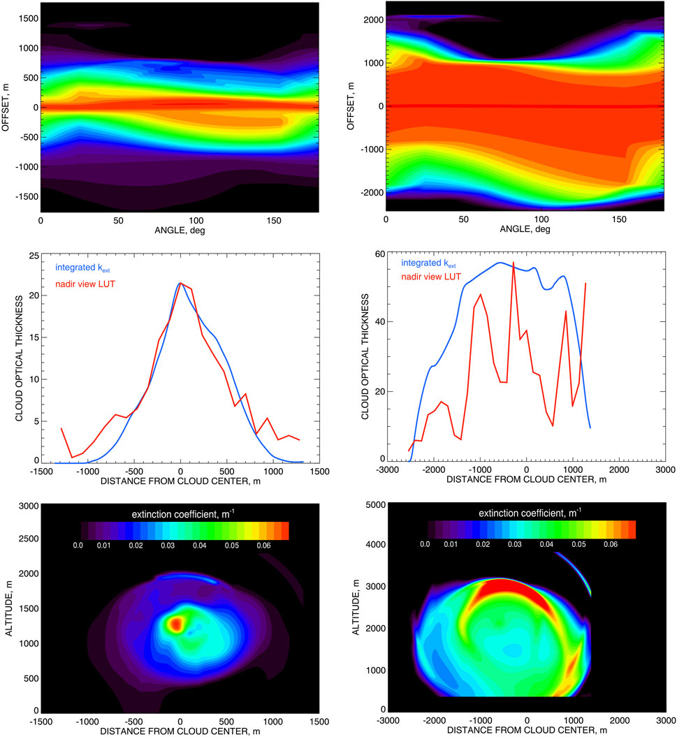
Figure 6. Top: The dCOT tomograms ${\tau }_{\text{tom}}(\psi ,\rho )$ derived from $R_{\text{tom}}(\psi ,\rho )$ shown in Figure 5 (bottom) using the proxy relation Equation 1 (no color bar is shown since the units here are arbitrary). Middle: COTs derived by application of the RSP LUT algorithm to nadir-view reflectances (red) and by integration of the backprojected $k_{\text{ext}}$ field subsequently scaled to match the RSP LUT COT maximum (blue). Bottom: The spatial distribution of the extinction coefficient derived from ${\tau }_{\text{tom}}$ using inverse Radon transform and calibrated by matching the RSP COT from middle plot. Left: Cloud 1 case from August 25; Right: Cloud 2 case from September 9.

dCOT tomogram can be used to define the “optical aspect ratio” of the cloud as

$A_{\text{opt}}=\frac{\max {\tau }_{\text{tom}}\left(90°,\rho \right)}{\max {\tau }_{\text{tom}}\left(0°,\rho \right)}.(2)$

It provides a single number independent of cloud shape corresponding to a specific reflectance threshold. These cloud shapes may have different aspect ratios as can be seen in Figure 4. For Cloud 1 $\max {\tau }_{\text{tom}}(90°,\rho )=0.1896$ and $\max {\tau }_{\text{tom}}(0°,\rho )=0.1870$. Note that despite both these numbers are defined up to a common arbitrary constant factor, their ratio $A_{\text{opt}}=1.014$ does not have this ambiguity.

4.4 Extinction coefficient density and its calibration

The initial extinction coefficient densities (extinction distributions) in both cases were computed by application of inverse Radon transform to the dCOT tomograms presented in Figure 6 (top). However, as we mentioned above, these distributions are defined up to an arbitrary constant factors and need to be calibrated. The calibration factor in each case has to be determined from an additional retrieved parameter. The most obvious candidate for such parameter is the COT derived from the RSP’s nadir reflectances using the standard operational procedure based on 1D-RT-computed LUT (see Section 2). The calibration procedure is illustrated in Figure 6 (middle). In these panels the COTs derived using the RSP’s nadir-view measurements are shown in red. The blue curves there depict the COTs computed by integration of the initial backprojected $k_{\text{ext}}$ field along vertical dimension. They are subsequently scaled to match their maxima with those of the corresponding RSP-LUT-derived COTs. Particularly good agreement between the shapes of the two COT curves is seen in Figure 6 (middle left) corresponding to Cloud 1. The scaling factors used to match the two curves in each plot are our calibration coefficients that are then applied to the initial extinction distributions resulting in the final retrievals shown in Figure 6 (bottom).

The problem with this calibration algorithm is in the bias of COT retrievals for isolated cloud in the presence of 3D radiative effects. Alexandrov et al. (2024) demonstrated using 3D RT simulations that COT retrievals made assuming a plane-parallel geometry can underestimate the actual values by a factor of four or even larger. This bias is primarily caused by leaking of scattered radiation through the cloud’s sides, which is not accounted for in LUT based on 1D RT computations. Alexandrov et al. (2024) suggested a simple linear formula for correction of the retrieved COT:

${\tau }_{\text{ren}}=\left(1+A\right){\tau }_{\text{meas}}.(3)$

Here ${\tau }_{\text{meas}}$ is the measured COT derived from the total nadir reflectance using LUT based on 1D RT and ${\tau }_{\text{ren}}$ is the renormalized COT value corrected for 3D radiative effects. The renormalization factor depends on the cloud aspect ratio

$A=\frac{H}{L},(4)$

where $H$ and $L$ are the cloud’s vertical and horizontal dimensions respectively. For irregularly shaped cloud these quantities can be defined as maxima of cloud extent in the corresponding directions. The correction formula Equation 3 with cloud aspect ratio defined by Equation 4 was extensively tested and validated by Alexandrov et al. (2024) using 3D RT simulations based on both realistic LES-generated and model “box” clouds. Theoretical basis for this renormalization procedure was provided by Alexandrov et al. (2025).

For moderate COT values $\lesssim 50$ scattering of light by large cloud droplets mostly occurs within the scattering plane so the radiation transfer within the cloud can be considered as two-dimensional. Note that in our cases the scattering plane coincides with the solar principal plane where the RSP makes its measurements, thus, $L$ is the along-track length of the cloud. Both $H$ and $L$ values can be estimated from Figures 5, 6 or derived using Equation 2. We see that for both clouds the aspect ratio $A\approx 1$ meaning that the RSP’s nadir-view-derived COTs (and, therefore, the cloud extinction coefficients) are underestimated by a factor of two. We adjusted the color bars in Figure 6 (bottom) accordingly. The same color bars are used in Figures 7, 8.

Figure 7

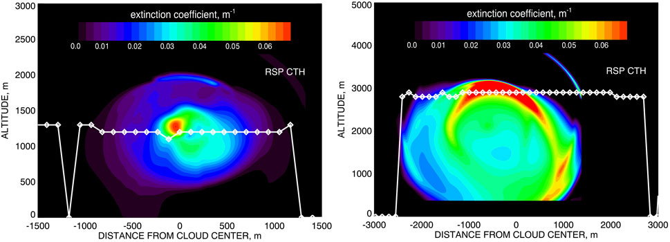
Figure 7. Same as Figure 6 (bottom) but with the RSP-derived cloud top heights (CTH) over-plotted in white. Left: Cloud 1 case from August 25; Right: Cloud 2 case from September 9.

Figure 8

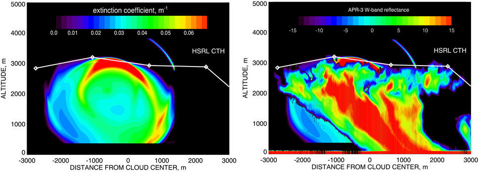
Figure 8. The extinction coefficient distribution in Cloud 2 case (Figure 6 (bottom right)) with over imposed cloud top height derived from HSRL-2 lidar data (left) and W-band reflectance field derived from APR-3 radar measurements (right).

4.5 Cloud top heights and comparison with other instruments

As we mentioned in Section 2, the RSP data processing includes an independent stereo block-correlation algorithm (Sinclair et al., 2017) for determination of cloud top heights (CTH). The results obtained using this algorithm are presented in Figure 7 as white lines plotted over the extinction densities from Figure 6 (bottom). We see a better agreement in CTH for Cloud 2 (right plot) probably because it is larger and optically denser (so our COT-based tomography is more robust).

CTH values are also available from the correlative lidar measurements made by HSRL-2 (Collow et al., 2022; Edwards et al., 2022; Christopoulos et al., 2025). These measurements were not available in the Cloud 1 case, while the results for Cloud 2 are presented in Figure 8 (left) being plotted over the extinction coefficient distribution from Figure 6 (bottom right). In Figure 8 (right) the W-band reflectance field derived from APR-3 radar measurements is also plotted over our extinction distribution. Good agreements (say, within 50 m) in CTH values can bee seen for all three instruments, except for the utmost right part of the plots where our tomographic retrievals cut the cloud’s shape short. Similar discrepancy is present also in Figure 7 (right). The high-resolution radar reflectance field from Figure 8 (right) can provide a possible explanation of this artifact. It shows that at 1,000 m from the center of the cloud it becomes physically (and therefore optically) thin, so while still visible in lidar and radar data (as well as in correlation-based RSP CTH), this part of the cloud was not detected by the dCOT-based tomography.

5 Conclusion

We presented examples of tomographic analyzes of real clouds observed by the RSP during NASA’s ${\text{CAMP}}^2$Ex field experiment conducted in the vicinity of the Philippines in 2019 during the Southeast Monsoon season. During this field campaign the RSP was deployed on-board of NASA’s P3-B aircraft together with a number of other remote-sensing and in situ instruments.

The original tomographic algorithm based on Radon transform and involving collection of cloud shapes corresponding to a number of brightness thresholds was described and validated in Part I of the series. In this study we resolved the issue with calibration of the derived 2D extinction density using the COT renormalization procedure introduced by Alexandrov et al. (2024).

Applicability of our tomographic algorithm to a specific cloud type depends on the cloud geometry that should allow for construction of cloud shapes using tangent view rays (see Section 4.1). The RSP measurements lack near-horizontal view rays, thus, constraining of cloud shape should not significantly rely on them. This means that our technique provides the best results either for “round”clouds (with aspect ratio close to one, e.g., Cu) and those having column-like shape (with higher aspect ratio, e.g., CuCg). Currently the clouds suitable for analysis are selected manually, however some crude preliminary cloud shape characterization may be developed in the future to make cloud selection more automated.

We demonstrated step-by-step performance of our tomographic algorithm on two examples from ${\text{CAMP}}^2$Ex: Cu cloud observed on August 25 and CuCg (Tcu) cloud observed on 9 September 2019. These cases are identified throughout the paper as Cloud 1 and Cloud 2 respectively. Finally, we presented comparisons of our retrievals with cloud top heights from three different sources: independent RSP block-correlation algorithm, lidar (HSRL-2), and radar (APR-3) measurements. The latter two instruments were deployed on the same platform as the RSP during ${\text{CAMP}}^2$Ex. High-resolution radar reflectance measurements provided detailed shape of Cloud 2 including a thin part that was missed in tomographic retrievals.

In our future work we plan to follow the framework of Part I and use the RSP’s polarimetric retrievals of droplet size distribution parameters to convert the extinction coefficients into droplet number concentrations. The latter will then be compared with in situ measurements made in the vicinity of our clouds. We also plan to further refine our algorithm and to consider more examples.

The tomographic algorithm described in this article relies on multi-angle measurements that are used to constrain cloud shapes. This means that it is applicable mostly to data from along-track scanners such as RSP and APS, as well as the proposed multispectral Scanning Polarimeter (ScanPol) (Milinevsky et al., 2019) and particulate observing scanning polarimeter (POSP) (Zhu et al., 2020). The most of imaging instruments make measurements at a single angle (usually at nadir), thus their data cannot be used as input for the tomographic technique presented in this study. The exception is the Hyper-Angular Rainbow Polarimeter (HARP) family of instruments, which have combined imaging and multi-angle capabilities. This family includes airborne AirHARP (McBride et al., 2024) and HARP-2 (Sienkiewicz et al., 2025) currently deployed on PACE satellite platform.

We currently work on a simplified parametric tomographic technique based on certain assumptions about cloud shape and extinction coefficient distribution. This technique does not require multiple view angles and can be applied to nadir-view measurements (including those from imagers). It is entirely analytical, thus, has computational efficiency sufficient for processing satellite data in real time. We plan to apply this technique to data from Ocean Color Imager (OCI) onboard PACE satellite.

Data availability statement

The raw data supporting the conclusions of this article will be made available by the authors, without undue reservation.

Author contributions

MA: Writing – original draft, Investigation, Software, Conceptualization, Writing – review and editing, Methodology. BVD: Writing – review and editing, Methodology, Funding acquisition, Resources, Data curation. BC: Resources, Data curation, Supervision, Methodology, Writing – review and editing, Funding acquisition. AW: Data curation, Software, Writing – review and editing.

Funding

The author(s) declare that financial support was received for the research and/or publication of this article. This research was funded by the NASA Radiation Sciences Program managed by Hal Maring and NASA grants NNH16ZDA001N-CAMP2EX and NNH19ZDA001N-PACESAT.

Acknowledgments

We are tremendously grateful to the ${\text{CAMP}}^2$Ex leadership team that allowed us to obtain such a comprehensive cloud remote sensing dataset. The NASA P-3B pilots, crew and management were immensely supportive and we thank them for all the help they so generously provided. We would like to thank R. Ferrare and C. Hostetler for providing HSRL-2 data. We are also indebted to S. Tanelli and the radar team at JPL for making APR-3 retrievals available to us.

Conflict of interest

Author AW was employed by Autonomic Integra LLC.

The remaining authors declare that the research was conducted in the absence of any commercial or financial relationships that could be construed as a potential conflict of interest.

The author(s) declared that they were an editorial board member of Frontiers, at the time of submission. This had no impact on the peer review process and the final decision.

Generative AI statement

The author(s) declare that no Generative AI was used in the creation of this manuscript.

Any alternative text (alt text) provided alongside figures in this article has been generated by Frontiers with the support of artificial intelligence and reasonable efforts have been made to ensure accuracy, including review by the authors wherever possible. If you identify any issues, please contact us.

Publisher’s note

All claims expressed in this article are solely those of the authors and do not necessarily represent those of their affiliated organizations, or those of the publisher, the editors and the reviewers. Any product that may be evaluated in this article, or claim that may be made by its manufacturer, is not guaranteed or endorsed by the publisher.

References

Alexandrov, M. D., Cairns, B., Emde, C., Ackerman, A. S., and van Diedenhoven, B. (2012a). Accuracy assessments of cloud droplet size retrievals from polarized reflectance measurements by the research scanning polarimeter. Remote Sens. Environ. 125, 92–111. doi:10.1016/j.rse.2012.07.012

CrossRef Full Text | Google Scholar

Alexandrov, M. D., Cairns, B., and Mishchenko, M. I. (2012b). Rainbow fourier transform. J. Quant. Spectrosc. Radiat. Transf. 113, 2521–2535. doi:10.1016/j.jqsrt.2012.03.025

CrossRef Full Text | Google Scholar

Alexandrov, M. D., Cairns, B., Wasilewski, A. P., Ackerman, A. S., McGille, M. J., Yorks, J. E., et al. (2015). Liquid water cloud properties during the polarimeter definition experiment (PODEX). Remote Sens. Environ. 169, 20–36. doi:10.1016/j.rse.2015.07.029

CrossRef Full Text | Google Scholar

Alexandrov, M. D., Cairns, B., Emde, C., Ackerman, A. S., Ottaviani, M., and Wasilewski, A. P. (2016a). Derivation of cumulus cloud dimensions and shape from the airborne measurements by the research scanning polarimeter. Remote Sens. Environ. 177, 144–152. doi:10.1016/j.rse.2016.02.032

CrossRef Full Text | Google Scholar

Alexandrov, M. D., Cairns, B., van Diedenhoven, B., Ackerman, A. S., Wasilewski, A. P., McGill, M. J., et al. (2016b). Polarized view of supercooled liquid water clouds. Remote Sens. Environ. 181, 96–110. doi:10.1016/j.rse.2016.04.002

CrossRef Full Text | Google Scholar

Alexandrov, M. D., Cairns, B., Sinclair, K., Wasilewski, A. P., Ziemba, L., Crosbie, E., et al. (2018). Retrievals of cloud droplet size from the research scanning polarimeter data: validation using in situ measurements. Remote Sens. Environ. 210, 76–95. doi:10.1016/j.rse.2018.03.005

CrossRef Full Text | Google Scholar

Alexandrov, M., Miller, D., Rajapakshe, C., Fridlind, A., van Diedenhoven, B., Cairns, B., et al. (2020). Vertical profiles of droplet size distributions derived from cloud-side observations by the research scanning polarimeter: tests on simulated data. Atmos. Res. 239, 104924. doi:10.1016/j.atmosres.2020.104924

PubMed Abstract | CrossRef Full Text | Google Scholar

Alexandrov, M. D., Emde, C., van Diedenhoven, B., and Cairns, B. (2021). Application of radon transform to multi-angle measurements made by the research scanning polarimeter: a new approach to cloud tomography. Part I: theory and tests on simulated data. Front. Remote Sens. 2, 791130. doi:10.3389/frsen.2021.791130

CrossRef Full Text | Google Scholar

Alexandrov, M., Cairns, B., Emde, C., and van Diedenhoven, B. (2024). Correction of cloud optical thickness retrievals from nadir reflectances in the presence of 3D radiative effects. Part I: concept and tests on 3D RT simulations. Front. Remote Sens. 5, 1397631. doi:10.3389/frsen.2024.1397631

CrossRef Full Text | Google Scholar

Alexandrov, M., Cairns, B., van Diedenhoven, B., and Emde, C. (2025). Correction of cloud optical thickness retrievals from nadir reflectances in the presence of 3D radiative effects. Part II: theory. J. Atmos. Sci. 82, 933–941. doi:10.1175/JAS-D-24-0209.1

CrossRef Full Text | Google Scholar

Cairns, B., Russell, E. E., and Travis, L. D. (1999). “Research scanning polarimeter: calibration and ground-based measurements,”. Polarization: measurement, analysis, and remote sensing. Editors D. H. Goldstein,, and D. B. Chenault (Proc. SPIE, Bellingham, WA), 3754, 186–197. doi:10.1117/12.366329

CrossRef Full Text | Google Scholar

Christopoulos, J. A., Saide, P. E., Ferrare, R., Collister, B., Barton-Grimley, R. A., Scarino, A. J., et al. (2025). Improving planetary boundary layer height estimation from airborne lidar instruments. J. Geophys. Res. Atmos. 130, e2024JD042538. doi:10.1029/2024jd042538

CrossRef Full Text | Google Scholar

Collow, A. B. M., Buchard, V., Colarco, P. R., da Silva, A. M., Govindaraju, R., Nowottnick, E. P., et al. (2022). An evaluation of biomass burning aerosol mass, extinction, and size distribution in GEOS using observations from CAMP²Ex. Atmos. Chem. Phys. 22, 16091–16109. doi:10.5194/acp-22-16091-2022

CrossRef Full Text | Google Scholar

Doicu, A., Doicu, A., Efremenko, D. S., and Trautmann, T. (2022a). Cloud tomographic retrieval algorithms I: surrogate minimization method. J. Quant. Spectrosc. Radiat. Transf. 277, 107954. doi:10.1016/j.jqsrt.2021.107954

CrossRef Full Text | Google Scholar

Doicu, A., Doicu, A., Efremenko, D. S., and Trautmann, T. (2022b). Cloud tomographic retrieval algorithms II: adjoint method. J. Quant. Spectrosc. Radiat. Transf. 285, 108177.

CrossRef Full Text | Google Scholar

Edwards, E.-L., Reid, J. S., Xian, P., Burton, S. P., Cook, A. L., Crosbie, E. C., et al. (2022). Assessment of NAAPS-RA performance in maritime southeast Asia during CAMP²Ex. Atmos. Chem. Phys. 22, 12961–12983. doi:10.5194/acp-22-12961-2022

CrossRef Full Text | Google Scholar

Emde, C., Buras, R., Mayer, B., and Blumthaler, M. (2010). The impact of aerosols on polarized sky radiance: model development, validation, and applications. Atmos. Chem. Phys. 10, 383–396. doi:10.5194/acp-10-383-2010

CrossRef Full Text | Google Scholar

Lee, B., Di Girolamo, L., Zhao, G., and Zhan, Y. (2018). Three-dimensional cloud volume reconstruction from the Multi-angle imaging SpectroRadiometer. Remote Sens. 10, 1858. doi:10.3390/rs10111858

CrossRef Full Text | Google Scholar

Levis, A., Schechner, Y. Y., Davis, A. B., and Loveridge, J. (2020). Multi-view polarimetric scattering cloud tomography and retrieval of droplet size. Remote Sens. 12, 2831. doi:10.3390/rs12172831

CrossRef Full Text | Google Scholar

Loveridge, J., Levis, A., Di Girolamo, L., Holodovsky, V., Foster, L., Davis, A. B., et al. (2023). Retrieving 3D distributions of atmospheric particles using atmospheric tomography with 3D radiative transfer – part 1: model description and Jacobian calculation. Atmos. Meas. Tech. 16, 1803–1847. doi:10.5194/amt-16-1803-2023

CrossRef Full Text | Google Scholar

Martin, W. G. K., and Hasekamp, O. P. (2018). A demonstration of adjoint methods for multi-dimensional remote sensing of the atmosphere and surface. J. Quant. Spectrosc. Radiat. Transf. 204, 215–231. doi:10.1016/j.jqsrt.2017.09.031

CrossRef Full Text | Google Scholar

Mayer, B. (2009). Radiative transfer in the cloudy atmosphere. Eur. Phys. J. Conf. 1, 75–99. doi:10.1140/epjconf/e2009-00912-1

CrossRef Full Text | Google Scholar

McBride, B. A., Martins, J. V., Cieslak, J. D., Fernandez-Borda, R., Puthukkudy, A., Xu, X., et al. (2024). Pre-launch calibration and validation of the airborne hyper-angular rainbow polarimeter (AirHARP) instrument. Atmos. Meas. Tech. 17, 5709–5729. doi:10.5194/amt-17-5709-2024

CrossRef Full Text | Google Scholar

Milinevsky, G., Oberemok, Y., Syniavskyi, I., Bovchaliuk, A., Kolomiets, I., Fesianov, I., et al. (2019). Calibration model of polarimeters on board the Aerosol-UA space mission. J. Quant. Spectrosc. Radiat. Transf. 229, 92–105. doi:10.1016/j.jqsrt.2019.03.007

CrossRef Full Text | Google Scholar

Mishchenko, M. I. (2006). “Glory,” in Earth science reference handbook: a guide to NASA’s Earth science program and Earth observing satellite missions. Editors C. L. Parkinson, A. Ward, and M. D. King (National Aeronautics and Space Administration, Washington, D.C.), 141–147.

Google Scholar

Mishchenko, M. I., Cairns, B., Kopp, G., Schueler, C. F., Fafaul, B. A., Hansen, J. E., et al. (2007). Accurate monitoring of terrestrial aerosols and total solar irradiance: introducing the glory mission. Bull. Amer. Meteorol. Soc. 88, 677–692. doi:10.1175/bams-88-5-677

CrossRef Full Text | Google Scholar

Nakajima, T., and King, M. D. (1990). Determination of the optical thickness and effective particle radius of clouds from reflected solar radiation measurements. Part I: theory. J. Atmos. Sci. 47, 1878–1893. doi:10.1175/1520-0469(1990)047<1878:dotota>2.0.co;2

CrossRef Full Text | Google Scholar

Radon, J. (1917). “Über die Bestimmung von Funktionen durch ihre Integralwerte längs gewisser Mannigfaltigkeiten,” in Berichte über die Verhandlungen der Königlich-Sächsischen Akademie der Wissenschaften zu Leipzig, Mathematisch-Physische Klasse (Leipzig: Teubner), 69, 262–277.

Google Scholar

Radon, J., and Parks, P. C. (1986). On the determination of functions from their integral values along certain manifolds. IEEE Trans. Med. Imaging 5, 170–176. doi:10.1109/tmi.1986.4307775

PubMed Abstract | CrossRef Full Text | Google Scholar

Reid, J., Maring, H., Narisma, G., van den Heever, S., Girolamo, L. D., Ferrare, R., et al. (2023). The coupling between tropical meteorology, aerosol lifecycle, convection, and radiation, during the cloud, aerosol and monsoon processes Philippines experiment (CAMP2Ex). Bull. Amer. Meteorol. Soc. 104, E1179–E1205. doi:10.1175/BAMS-D-21-0285.1

CrossRef Full Text | Google Scholar

Sienkiewicz, N., Martins, J. V., McBride, B. A., Xu, X., Puthukkudy, A., Smith, R., et al. (2025). HARP2 pre-launch calibration: dealing with polarization effects of a wide field of view. Atmos. Meas. Tech. 18, 2447–2462. doi:10.5194/amt-18-2447-2025

CrossRef Full Text | Google Scholar

Sinclair, K., van Diedenhoven, B., Cairns, B., Yorks, J., Wasilewski, A., and McGill, M. (2017). Remote sensing of multiple cloud layer heights using multi-angular measurements. Atmos. Meas. Tech. 10, 2361–2375. doi:10.5194/amt-10-2361-2017

CrossRef Full Text | Google Scholar

Sinclair, K., van Diedenhoven, B., Cairns, B., Alexandrov, M., Moore, R., Crosbie, E., et al. (2019). Polarimetric retrievals of cloud droplet number concentrations. Remote Sens. Environ. 228, 227–240. doi:10.1016/j.rse.2019.04.008

CrossRef Full Text | Google Scholar

Tzabari, M., Holodovsky, V., Shubi, O., Eytan, E., Koren, I., and Shechner, Y. Y. (2022). Settings for spaceborne 3-D scattering tomography of liquid-phase clouds by the CloudCT mission. IEEE Trans. Geosci. Remote. Sens. 60, 1–16. doi:10.1109/tgrs.2022.3198525

CrossRef Full Text | Google Scholar

Werdell, P. J.Coauthors (2019). The plankton, aerosol, cloud, ocean ecosystem (PACE) mission: status, science, advances. Bull. Amer. Meteor. Soc. 100, 1775–1794.

Google Scholar

Zhu, S., Hong, J., Li, Z., Lei, X., Zou, P., Liu, Z., et al. (2020). Radiometer-to-imager in-flight cross calibration and verification. Opt. Express 28, 11001–11015. doi:10.1364/OE.386566

PubMed Abstract | CrossRef Full Text | Google Scholar