Performance of glint correction algorithms for Sentinel-3 OLCI data

Sentinel-3 (A/B) Ocean and Land Colour Imager (OLCI) provides daily global coverage and spectral quality for monitoring optical water quality indicators across diverse aquatic systems. Accurate retrieval of remote sensing reflectance (R_rs) from OLCI imagery requires a series of radiometric correction procedures. Specifically, glint correction algorithms are essential in accounting for the impact of specular reflections from sunlight and skylight at the air-water interface, which can distort the radiance measured at the satellite sensor. Despite its importance, the performance of glint correction algorithms remains underexplored for Sentinel-3 (A/B) OLCI imagery and represents a research gap for its application. In this study, we analyzed the principles and performance of three image-based sunglint correction algorithms and one skyglint correction method across varying intensities of glint effects, using 570 Sentinel-3 (A/B) OLCI imagery acquired between 2020 and 2024. Resulting R_rs retrievals were evaluated against the Aerosol Robotic Network for Ocean Color (AERONET-OC) observations at 11 coastal sites. All proposed sunglint correction methods improved R_rs retrievals compared to no glint correction over various optical water types. Among them, the combination of SCSh (i.e., a sunglint removal method designed for optically shallow waters) and SkyG (i.e., an analytical skyglint removal method) achieved the best overall performance, yielding the lowest absolute error (ε < 58%) and the smallest number of spectra that were significantly overcorrected (n = 99), However, challenges remain in the blue spectral range (400–490 nm), where the glint correction methods performed poorly compared to AERONET-OC observations, especially under medium and high-glint conditions. Moreover, glint-free images were overcorrected for all methods, highlighting the need for reliable glint detection and masking before applying corrections. Our findings demonstrated that while existing glint correction methods can significantly improve data quality under low and medium-glint conditions, the high-glint scenarios continue to pose difficulties. Addressing these limitations is essential to ensure the consistent and accurate use of the Sentinel-3 (A/B) OLCI data for aquatic monitoring.

1 Introduction

Satellite observations play a crucial role in improving the monitoring of aquatic systems. Since the launch of the Coastal Zone Color Scanner (CZCS) in 1978, the first ocean color mission, there have been significant advancements in understanding and correcting atmospheric effects and other factors affecting satellite imagery (Gordon, 2021). Advancements in sensor design and technology have enabled the development of new capabilities over time, leading to significant improvements in spectral, radiometric, and spatial resolution to better address the complexities of aquatic systems (Dierssen et al., 2021). The Sentinel-3 mission, jointly operated by the European Space Agency (ESA) and EUMETSAT, has provided daily aquatic observations since its launch in April 2016, through a constellation of two Ocean and Land Colour Imager (OLCI) sensors (A/B) (Donlon et al., 2012). OLCI captures imagery at 300 m spatial resolution across 21 spectral bands, spanning wavelengths from 400 to 1,020 nm in the visible to near-infrared range, with a high signal-to-noise ratio in visible bands. These capabilities have supported a wide range of aquatic applications in inland, coastal, and open ocean waters (Mishra et al., 2019; Pahlevan et al., 2020; Warren et al., 2021), including monitoring of water clarity and turbidity (Vanhellemont and Ruddick, 2021; Shen et al., 2020; Warren et al., 2021), derivation of water’s inherent optical properties (Xue et al., 2019), analysis of trends in phytoplankton community size (Liu et al., 2021), and forecasting (Schaeffer et al., 2024) and generation of synthetic images (Paulino et al., 2025) for monitoring cyanobacterial harmful algal blooms. Given its open-access nature and broad applicability, Sentinel-3 (A/B) OLCI serves as a valuable data source for aquatic remote sensing, and this study focuses on revisiting sunglint and skyglint (or only glint) correction methodologies to contribute to the reliability and quality of its products.

Glint effects occur from specular reflections of sunlight and skylight at the air-water interface, directed toward the satellite sensor, bypassing interactions with the water column (Cox and Munk, 1954; Kay et al., 2009; Mobley, 2015). These effects are primarily influenced by the state of surface water (i.e., roughness) as well as solar and sensor viewing geometries (Cox and Munk, 1954; Mobley, 2015). Though independent, both sunglint and skyglint can introduce dramatic spectral distortions in satellite imagery. Because glint contributions can far exceed the water-leaving radiance at the Top-Of-Atmosphere (TOA), they represent a dominant source of radiometric distortion in optical satellite imagery over water, affecting the estimations of key Optically Active Components (OACs) such as phytoplankton, colored dissolved organic matter (CDOM), and non-algal particles (NAP) (Kirk, 2011) – thereby limiting the usability of satellite images (Goodman et al., 2008). Thus, correcting or masking out these effects is essential in aquatic applications. Sentinel-3 (A/B) OLCI operates with a 12.6° westward across-track to reduce the sunglint effects (Donlon et al., 2012). However, glint contamination remains a prevalent issue in OLCI imagery (de Lima et al., 2025; Mishra et al., 2019; Paulino et al., 2025), which shows the need for efficient corrections.

Diverse glint removal algorithms, commonly referred to as “deglint” methods, are used in ocean color applications. The most established deglint approach is based on the Cox and Munk model (Cox and Munk, 1954; Cox and Munk, 1955), a statistical method that estimates sunglint radiance contributions using wind speed and direction characteristics. While this method is well-established and widely adopted for medium and coarse-resolution (>100 m) ocean color sensors (Wang and Bailey, 2001), its accuracy is highly dependent on wind speed data, which is a major source of uncertainty and limitation (Chen et al., 2021; Bréon and Henriot, 2006; Fukushima et al., 2009). In contrast, image-based deglint methods have gained increasing popularity in recent decades (Giles et al., 2021; Harmel et al., 2018; Hedley et al., 2005; Kutser et al., 2009; Vanhellemont, 2019). These methods offer several advantages, including (i) they do not rely on water surface roughness assumptions, instead estimating the sunglint signal using specific wavelengths with negligible water signal (e.g., near-infrared and shortwave infrared), (ii) they are broadly applicable because they do not depend on external data (i.e., wind speed/direction), and (iii) they can be easily integrated into operational workflows without significant computational costs. Skyglint removal methodologies, in contrast, are primarily based on Rayleigh-type atmospheric scattering models (Gordon et al., 1988; Vanhellemont and Ruddick, 2018) and are more straightforward compared to sunglint correction techniques. However, validation analyses for glint correction methods in Sentinel-3 (A/B) OLCI images remain scarce, and this gap in validation raises an important and still unresolved question: “Can these deglint methods be reliably applied to correct glint effects in 300 m Sentinel-3 (A/B) OLCI images?”

To address this question, we implemented and validated the three image-based sunglint correction algorithms in 570 Sentinel-3 (A/B) OLCI imagery (2020–2024) under different intensities of glint effects and optical water types. The estimated OLCI R_rs were validated using globally distributed Aerosol Robotic Network for Ocean Color (AERONET-OC) match-up observations at 11 coastal sites. Additionally, we applied a skyglint correction approach together with the sunglint correction to evaluate the potential benefits. Until now, this study has been the most comprehensive assessment of glint correction methods for Sentinel-3 (A/B) OLCI. It analyzes the effectiveness of the approaches under distinct conditions and contributes to building consensus on the best-performing method. A detailed methodology is provided in Section 2. The main results are presented in Section 3, structured into four subsections covering sun and skyglint corrections. The key findings and recommendations are discussed in Section 4, followed by the conclusions in Section 5.

2 Materials and methods

2.1 Sentinel-3 (A/B) OLCI images

Sentinel-3 (A/B) OLCI has provided daily ocean color data since 2016, capturing 21 narrow spectral bands along the visible to near-infrared wavelengths (400–1,020 nm) with a high signal-to-noise ratio (range: 605–2,188 in visible wavelengths) and 14-bit radiometric resolution (Donlon et al., 2012). The OLCI sensor operates in a near-polar, sun-synchronous orbit at an altitude of 815.5 km, crossing the equator at approximately 10:00 a.m. local time. OLCI offers images with a spatial resolution of 300 m and a wide swath of 1,270 km, tilted 12.6° westwards to minimize the sunglint effect. In this study, we utilized Sentinel-3 (A/B) OLCI imagery acquired between 2020 and 2024 (5 years), alongside match-up in situ observations from the AERONET-OC. Sentinel-3 OLCI EFR Level-1 images were acquired, providing calibrated, geolocated, and spatially resampled Top-Of-Atmosphere (TOA) radiances, and then corrected for atmospheric and glint effects (see Section 2.3; Section 2.4). To mitigate the cloud-related artifacts, including shadows and adjacency effects (Feng and Hu, 2016), only cloud-free scenes within a 100-by-100 km window centered on the AERONET-OC sites were selected. Additionally, the images were filtered according to the spectral distortion degree (Section 2.5). Out of the 3,494 verified images, a total of 570 Sentinel-3 (A/B) OLCI images were retained for analysis. For validation purposes, we focused on eight spectral bands (i.e., 400, 413, 443, 490, 510, 560, 620, and 665 nm) that aligned with AERONET-OC observations (Figure 1c).

Figure 1

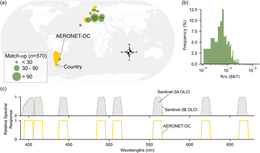
Figure 1. (a) AERONET-OC sites and match-ups (n = 570). (b) Frequency distribution of (log-scale) R_rs (667) obtained from AERONET-OC data. (c) Relative Spectral Response for eight bands of Sentinel-3 (A/B) OLCI and AERONET-OC used for validation. Details about AERONET-OC sites used in this study are available in Table A1 (Supplementary Appendix A).

2.2 Aerosol Robotic Network-ocean color (AERONET-OC)

AERONET-OC is a global network of autonomous above-water radiometers deployed on fixed platforms in inland, coastal, and open ocean waters (Zibordi et al., 2006). For over 2 decades, it has continuously provided records of normalized water-leaving radiance (nLW) and has been widely used to validate a range of ocean color sensors and image-processing approaches (Zibordi et al., 2022; Pahlevan et al., 2021; Melin, 2022; Paulino et al., 2026). Here, we used AERONET-OC Version 3 Level 2.0 data from 11 sites (from 2020 to 2024), with a timeframe of approximately 1.5 h relative to the Sentinel-3 (A/B) OLCI overpass. Match-ups were defined as cloud-free satellite observations (Section 2.1) that spatially and temporally corresponded to AERONET-OC measurements. Figure 1 presents the geographic locations of the AERONET-OC sites and highlights the dataset’s spectral variability through the aquatic reflectance values at 667 nm. The nLW measurements, acquired across the visible spectrum (400–665 nm), were converted to remote sensing reflectance (R_rs, sr⁻¹) by dividing them by the extra-terrestrial solar irradiance (Thuillier et al., 2003) and subsequently adjusted to match the Sentinel-3 (A/B) OLCI bandwidths and central wavelengths using OWT-based linear coefficients. A detailed description of the processing procedures for AERONET-OC data is provided in Paulino et al. (2026). The number of match-ups may vary regarding the number of spectral bands due to differences in the spectral AERONET-OC station settings (Zibordi et al., 2021).

2.3 Atmospheric correction of Sentinel-3 (A/B) OLCI

The atmospheric effect arises from the absorption and scattering of various atmospheric components (Gordon and Wang, 1994a; Gordon, 1997; Vermote et al., 1997), making its removal from satellite images essential for aquatic applications. In aquatic systems, the total signal, TOA reflectance (${\rho }_{TOA}$), can be simplified as the sum of Rayleigh-Aerosol reflectance (${\rho }_{R+A}$), glint effect (${\rho }_g$), and aquatic reflectance (${\rho }_w$), which is the primary objective of atmospheric correction (Equation 1):

${\rho }_{\text{TOA}}=\left[{\rho }_{R+A}+{\rho }_g+t{\rho }_w\right]T_g(1)$

Where t represents the atmospheric diffuse transmission described by Gordon and Wang (1994a) and $T_g$ is the gaseous transmission by water vapor, ozone, and other atmospheric gases. This formulation assumes that adjacency effects (Paulino et al., 2022), as well as the foam and whitecap contributions from the water surface are negligible. This assumption was supported by the characteristics of our selected match-ups, which were limited to cloud-free scenes (Section 2.1) and water pixels located, on average, 17 km from the nearest coastline according to the AERONET-OC station locations, with only three stations situated closer than 3 km, and exhibiting an average aerosol optical thickness of ∼0.11. Under such conditions, adjacency contamination is expected to be minimal (Bulgarelli et al., 2014; Bulgarelli and Zibordi, 2018; Paulino et al., 2022). In addition, all selected Sentinel-3 (A/B) OLCI images were visually inspected to confirm the absence of bright foam streaks or land artifacts, and the spectral shape analysis (Section 2.5) further confirmed this by filtering out any spectrally flat or non-physical signatures associated with foam coverage and whitecaps at visible range (Frouin et al., 1996; Gordon and Wang, 1994b). The ${\rho }_{R+A}$ term was derived using the 6SV radiative transfer model (Kotchenova et al., 2006; Vermote et al., 2006). The 6SV model incorporates prior atmospheric and image data to simulate spectral distortions in satellite images caused by multiple interactions between atmospheric optical components and light. This model is broadly used in land applications but also provides consistent results in aquatic studies (Bassani et al., 2016; Paulino et al., 2025; Pahlevan et al., 2020; Vanhellemont and Ruddick, 2018). In our case, input parameters for the 6SV model included aerosol optical thickness, water vapor, ozone, and altitude data obtained from AERONET-OC. Since AERONET-OC does not provide aerosol optical thickness at 550 nm, these values were interpolated to 550 nm using quadratic fits on a log-log scale (Eck et al., 1999). Additional parameters related to illumination and viewing geometry were extracted from Sentinel-3 (A/B) OLCI metadata. For aerosol characterization, the default 6SV aerosol models (Continental and Maritime) were used, distinguishing between aquatic ecosystems: inland (Continental), coastal (Maritime), and open ocean (Maritime) waters. The ${\rho }_g$ term is discussed in Section 2.4.

2.4 Proposed glint removal methods

In this study, three sunglint removal algorithms (Vanhellemont, 2019; Kutser et al., 2009) based on assumptions derived from satellite images were compared. These algorithms were integrated with an analytical approach to mitigate skyglint effects (Gordon et al., 1988). The sunglint methods were selected considering the image-based concept and their potential for implementation in operational workflows and efficient product generation without significant computational costs or additional data sources. Although statistically based methods may also perform well (Kay et al., 2009), their evaluation was beyond the scope of this study, which focuses on the central principle of image-based solutions already represented by the methods included in our analysis. All selected methods were applied to the atmospherically corrected images with glint (${\rho }_w^{*}$) (i.e., Equation 1 with ${\rho }_g=0$), using a consistent baseline atmospheric correction derived from 6SV to ensure inter-comparability of results. Overall, our validation framework (Figure 2) combined AERONET-OC observations, glint intensity derived from Sentinel-3 (A/B) OLCI images, and Optical Water Types (OWTs).

Figure 2

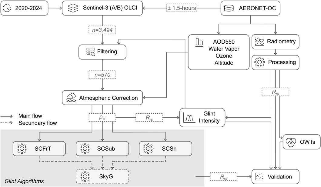
Figure 2. Overall framework for validating glint correction algorithms applied to Sentinel-3 (A/B) OLCI.

2.4.1 SCFrT: Sunglint correction based on fresnel reflectance and atmospheric transmittance using single-band assumption in longer wavelengths

The SCFrT method is defined to correct sunglint effects in higher spatial resolution sensors (e.g., 30 m Landsat and 10 m Sentinel-2) (Vanhellemont, 2019). Like other sunglint correction techniques (Cox and Munk, 1955; Harmel et al., 2018), SCFrT uses the Fresnel reflectance ($r$), which quantifies the proportion of sunlight reflected at the air-water interface. Fresnel reflectance is determined by the water’s refractive index (n), wavelength (λ), and incident angle of sunlight that reaches a wave facet (ω), which is directly correlated to the view and sun zenith angles. The correction of ${\rho }_g$ term in this approach is defined as Equations 2, 3:

${\rho }_w\left(\lambda \right)={\rho }_w^{*}\left(\lambda \right)-{\rho }_g\left(\lambda \right)(2)$

${\rho }_g\left(\lambda \right)={\rho }_w^{*}\left({\lambda }_{ref}\right)·\frac{T\left(\mathrm{\lambda }\right)}{T\left({\mathrm{\lambda }}_{ref}\right)}·\frac{r\left(\mathrm{\omega },n,\mathrm{\lambda }\right)}{r\left(\mathrm{\omega },n,{\mathrm{\lambda }}_{ref}\right)}(3)$

To capture the spectral variation of sunglint, SCFrT uses two ratios relative to a reference wavelength. The first ratio accounts for the fact that sunglint is primarily associated with the direct transmittance (T) of the sunlight, compensating for atmospheric attenuation across the spectrum. The second ratio adjusts for the wavelength-dependent variation in Fresnel reflectance. This method assumes a reference wavelength where water is effectively “dark” (i.e., ${\rho }_w^{*}\left({\lambda }_{ref}\right)=0$), meaning that any observed signal at this wavelength originates from sunglint. This assumption is based on strong water absorption at the reference wavelength, minimal interference from water’s OACs, and low atmospheric diffuse scattering (Harmel et al., 2018). While SCFrT originally uses shortwave-infrared bands (>1,600 nm) as a reference, we adopted the spectral band centered at 1,020 nm to align with the visible to near-infrared range of Sentinel-3 (A/B) OLCI. Additionally, the refractive index n was obtained following (Paulino et al., 2025), and T was derived using 6SV modeling (Section 2.3).

2.4.2 SCSub: Sunglint correction using a direct SUBtraction from longer wavelengths

The SCSub method relies on longer wavelengths and is widely used to remove sunglint effects in aquatic-environment satellite imagery, particularly in turbid waters (Begliomini et al., 2023; Lobo et al., 2014; Maciel et al., 2021). Like SCFrT, it assumes that the shortwave infrared region is strongly absorbed by water and can be utilized in the atmospheric correction (Wang and Shi, 2007; Gordon, 1997), including for removal of sunglint. For this method, any residual signal in this spectral range after atmospheric correction is attributed to sunglint. SCSub further assumes that the sunglint contribution is independent of wavelength and that the amount of sunglint observed in the shortwave infrared is directly related to its contribution in the visible and near-infrared bands. Therefore, to correct this effect, SCSub applies a simple subtraction of the shortwave infrared bands (>1,600 nm) across the visible and near-infrared ranges (similar to that suggested by Mueller and Austin (1995)). In our case, SCSub has been adapted for Sentinel-3 (A/B) OLCI images by considering the spectral band centered at 1,020 nm as a reference.

2.4.3 SCSh: A sunglint correction method for optically SHallow waters

The SCSh method is an empirical approach designed to address sunglint contamination in optically shallow waters, where bottom reflectance significantly influences the near-infrared range (Kutser et al., 2009). SCSh was developed for hyperspectral image applications, and it advances previous sunglint correction techniques that rely on near-infrared-based assumptions (Hedley et al., 2005). SCSh uses the oxygen absorption feature near 760 nm to estimate and correct sunglint contributions, assuming that the magnitude of this effect is proportional to the observed signal. Here, the sunglint-corrected aquatic reflectance is computed as Equations 4, 5:

${\rho }_w\left(\lambda \right)={\rho }_w^{*}\left(\lambda \right)-G\left(\lambda \right)·\frac{D}{D_{\mathit{max}}}(4)$

$D\left({\lambda }^0\right)=\frac{{\rho }_w^{*}\left({\lambda }^{-1}\right)+{\rho }_w^{*}\left({\lambda }^{+1}\right)}{2}-{\rho }_w^{*}\left({\lambda }^0\right)(5)$

The sunglint contribution is modeled using the glint intensity factor (D) and a pure glint spectrum extracted from the image itself (G). The ratio $\frac{D}{D_{\mathit{max}}}$ represents the depth of the oxygen absorption feature at ${\lambda }^0$, normalized by its maximum value. For Sentinel-3 (A/B) OLCI, the spectral bands centered at 754 nm, 761 nm, and 768 nm correspond to ${\lambda }^{-1}$, ${\lambda }^0$, and ${\lambda }^{+1}$, respectively. Values of $D$ close to zero indicate minimal or no sunglint contamination, while higher values correspond to increased sunglint. $G\left(\lambda \right)$ scales the correction across each spectral band, and it is estimated by subtracting the water spectrum at the minimum glint intensity ($D\left({\lambda }^0\right)$ min) from the water spectrum at the maximum glint intensity ($D\left({\lambda }^0\right)$ max). To refine the selection of G, land and cloud-contaminated pixels were removed using a near-infrared band reflectance threshold (${\rho }_w^{*}\left(1020\right)>0.13$), ensuring that sunglint effects at higher intensities are still retained for our analysis. This threshold was empirically defined through visual inspection of multiple images acquired under varying glint conditions.

2.4.4 SkyG: An analytical SKYGlint removal

In this validation scheme, we applied a skyglint correction to Sentinel-3 (A/B) OLCI images, combining it with three proposed sunglint correction algorithms. Skyglint is primarily associated with Rayleigh scattering and tends to introduce more significant distortions at shorter wavelengths, particularly in the blue range. A method for correcting these distortions is SkyG, an adaptation from Gordon et al. (1988), which accounts for the influence of the sun and sensor positions, Fresnel reflectance, and the atmospheric scattering phase function. This correction is expressed as Equations 6–8:

${\rho }_{sky}^g\left(\lambda \right)=\frac{{\tau }_r·[(r\left({\theta }_v,n,\lambda \right)+r({\theta }_s,n,\lambda ))·P_r({\theta }_{+})]}{4·\mathit{cos}{\theta }_s·\mathit{cos}{\theta }_v}(6)$

$P_r\left({\theta }_{+}\right)=\frac{3}{4}·\left(1+co{s}^2{\theta }_{+}\right)(7)$

$\mathit{cos}{\theta }_{+}=-\mathit{cos}{\theta }_s\mathit{cos}{\theta }_v-\mathit{sin}{\theta }_s\mathit{sin}{\theta }_v\cos \Delta \varphi (8)$

Where $r$ is the Fresnel reflectance at the air-water interface for the solar (${\theta }_s$) and view (${\theta }_v$) zenith angles, $\Delta \varphi$ is the relative azimuth angle, ${\tau }_r$ represents the Rayleigh scattering optical thickness, and $P_r$ is the Rayleigh scattering phase function, which characterizes the scattering of skylight by atmospheric gases and molecules as a function of the scattering angle (${\theta }_{+}$). The ${\tau }_r$ term was modeled using 6SV (Section 2.3), while the solar and view angles were retrieved from the Sentinel-3 (A/B) OLCI image metadata. The ${\rho }_{sky}^g$ component was spectrally subtracted from the aquatic reflectance after applying the sunglint correction.

2.5 Classification of the relative glint intensity in Sentinel-3 (A/B) OLCI images

To evaluate glint removal across the selected algorithms, we classified glint intensity into four levels – no-glint, low, medium, and high – based on the spectral similarity between Sentinel-3 (A/B) OLCI and AERONET-OC data. To minimize atmospheric uncertainties, all scenes were processed using the same atmospheric correction baseline, with parameters derived from AERONET (Section 2.3). Within this framework, the no-glint category serves as a reference to verify the consistency of the atmospheric correction, ensuring that the differences observed across glint levels primarily reflect variations in glint intensity rather than residual atmospheric effects (Figure 4). The OLCI R_rs medium spectrum (Section 2.7) extracted at the station located was compared to the match-up AERONET-OC spectrum, which serves as the reference. Glint effects are expected to introduce a positive offset across the spectrum with minimal impact on its shape, although skyglint may cause some distortions in the blue wavelengths. Glint levels were estimated using the Spectral Angle Mapper (d) metric (Kruse et al., 1993) (Equation 9), which quantifies discrepancies in spectral shape between the image and reference spectra. Additionally, the ratio (R) between the two spectra was used to assess glint magnitude (Equations 10, 11):

$d={\cos }^{-1}\left(\frac{{\displaystyle {\sum }_{i=1}^i}〈n{R}_w^0,n{R}_w^1〉}{{\left({\displaystyle {\sum }_{i=1}^i}{\left(n{R}_w^0\right)}^2\right)}^{1/2}{\left({\displaystyle {\sum }_{i=1}^i}{\left(n{R}_w^1\right)}^2\right)}^{1/2}}\right)(9)$

$n{R}_w=\frac{R_{rs}}{{\left[{\displaystyle {\sum }_{i=1}^i}{\left(R_{rs}\right)}^2\right]}^{1/2}}(10)$

$R=\frac{{\displaystyle {\sum }_{i=1}^i}{R}_{rs}^1}{{\displaystyle {\sum }_{i=1}^i}{R}_{rs}^0}(11)$

Where $R_{rs}$ refers to the spectrum of remote sensing reflectance (Section 2.7), $〈n{R}_w^0,n{R}_w^1〉$ represents the product of the normalized reflectance spectrum ($n{R}_w$) for AERONET-OC (0) and Sentinel-3 (A/B) OLCI (1), and i is the number of spectral bands. A d value close to zero indicates high similarity in spectral shapes, while lower values of R suggest more remarkable similarity in magnitude between the spectra. Our dataset (n = 570) was divided into four glint levels: no-glint (n = 18), low (168), medium (237), and high (147), considering the intervals of d ≤ 0.5 AND R ≤ 1.1; 1.1 < R ≤ 2; 2 < R ≤ 3, and R > 3, respectively. Figure 3 illustrates the classification criteria and glint intensities over Sentinel-3 (A/B) OLCI images and their corresponding spectra. Notably, the glint effect becomes visible in Sentinel-3 (A/B) OLCI images at medium and high intensities. This classification revealed that approximately 97% of Sentinel-3 (A/B) OLCI images acquired under cloud-free conditions were affected by some level of glint, reinforcing the importance of this study. Nonetheless, low and medium glint levels accounted for nearly 71% of the dataset, showing that most detected effects were not indicative of severe contamination.

Figure 3

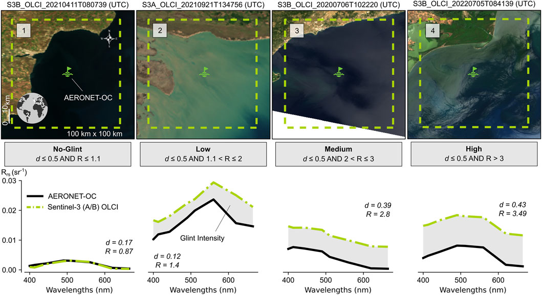
Figure 3. Glint intensities from Sentinel-3 (A/B) OLCI images and spectral shifts related to AERONET-OC observations.

2.6 Optical water types

We also analyzed the performance of glint correction algorithms across various optical water types. OWTs classify water masses based on their optical properties, encompassing both radiometric and biogeochemical parameters related to water composition. These parameters include Secchi disk depth, algae concentration, inorganic particles, and colored dissolved organic matter (Baker and Smith, 1982; Moore et al., 2014; Spyrakos et al., 2018). For this study, we used a set of 23 OWTs provided by Wei et al. (2022), which capture a wide range of optical water complexities, from low to high. In this context, low optical complexity corresponds to clear waters with minimal suspended and dissolved particles, typically found in oceanic waters, while high optical complexity is associated with productive and turbid waters, such as inland and coastal waters (Morel and Prieur, 1977). To simplify the classification of OWTs, we grouped them into five distinct categories (A, B, C, D, and E) using the k-means algorithm (Lloyd, 1982). Group A (OWTs: 1, 2, 3, and 4) represents waters with low optical complexity. Groups B (OWTs: 5, 6, 7, and 8), C (OWTs: 9, 10, 11, 12, and 13), and D (OWTs: 14, 15, 16, 17, and 18) correspond to intermediate optical conditions, while Group E (OWTs: 19, 20, 21, 22, and 23) includes waters with high optical complexity. Further detailed descriptions about the OWT groups are available in Paulino et al. (2026).

2.7 Validation

To ensure consistency with AERONET-OC observations, Sentinel-3 (A/B) OLCI images were transformed from ${\rho }_w$ to R_rs by dividing by π. For the Sentinel-3 (A/B) OLCI pixel extraction, median R_rs spectral data were taken from a 3-by-3 window (equivalent to 900 × 900 m) centered on AERONET-OC sites, excluding the central pixel to avoid platform-induced contamination. For the performance analysis, a set of statistics was calculated to describe the differences between Sentinel-3 (A/B) OLCI and AERONET-OC. The primary metrics included the median symmetric accuracy (ε), symmetric signed percentage bias (β) (Equations 12, 13), and spectral similarity metric d (Section 2.5). ε and β are log-transformed metrics used to minimize problems with outliers and asymmetry (Morley, 2016; Morley et al., 2018), and they are expressed in %. Additional metrics were also considered, such as Mean Absolute Percentage Error (MAPE) and Root Mean Square Error (RMSE) (Equations 14, 15).

$\epsilon \left(\%\right)=100\times \left({10}^Q-1\right)(12)$

$\beta \left(\%\right)=100\times sign\left(Z\right)\left({10}^{\left|Z\right|}-1\right)(13)$

$\text{MAPE}\left(\%\right)=\frac{1}{n}{\displaystyle \sum _{i=1}^n}\left|\frac{M_i-O_i}{M_i}\right|\times 100(14)$

$RMSE\left(s{r}^{-1}\right)=\sqrt{\frac{1}{n}{\displaystyle \sum _{i=1}^n}{\left(M_i-O_i\right)}^2}(15)$

Where M and O refer to measured (AERONET-OC) and observed (Sentinel-3 (A/B) OLCI) values, respectively, n is the sample size, and i represents the spectral bands. $\left(Z=Median\left({\log }_{10}\left(\frac{O_i}{M_i}\right)\right)\right)$ and $\left(Q=Median\left|{\log }_{10}\left(\frac{O_i}{M_i}\right)\right|\right)$. The validation metrics in this study are presented as the average calculated across all eight spectral bands to provide an overall assessment of the deglint method’s performance.

3 Results

3.1 Performance of sunglint removal algorithms under different glint intensities

Scatterplots in Figure 4 compare the R_rs values derived from Sentinel-3 (A/B) OLCI against AERONET-OC observations for three sunglint removal algorithms across varying glint intensities (i.e., No-Glint, Low, Medium, and High). All three methods improved the quality of Sentinel-3 (A/B) OLCI data compared to uncorrected images, especially in the presence of sunglint effect. Under low-glint conditions, SCSub presented the lowest errors, with absolute error (ε) and bias (β) around 37% and 34%, respectively, indicating stronger agreement with spectral content of AERONET-OC. As glint levels increased, all algorithms exhibited greater discrepancies in relation to in situ observations. The high-glint condition produced the most substantial deviations, with both ε and β exceeding 180%. Overall, SCSub achieved the best performance (ε < 85%), while SCFrT and SCSh showed close results, differing by less than 2% (see Fig. A2, Supplementary Appendix A. However, SCSub and SCSh maintained the most consistent performance across glint intensities, with satisfactory results from low to high-glint conditions. In contrast, SCFrT performance degraded under high-glint. Under no-glint images, SCFrT and SCSh were the best-performing models (β < 28%), suggesting that both effectively preserve the water’s spectral response.

Figure 4

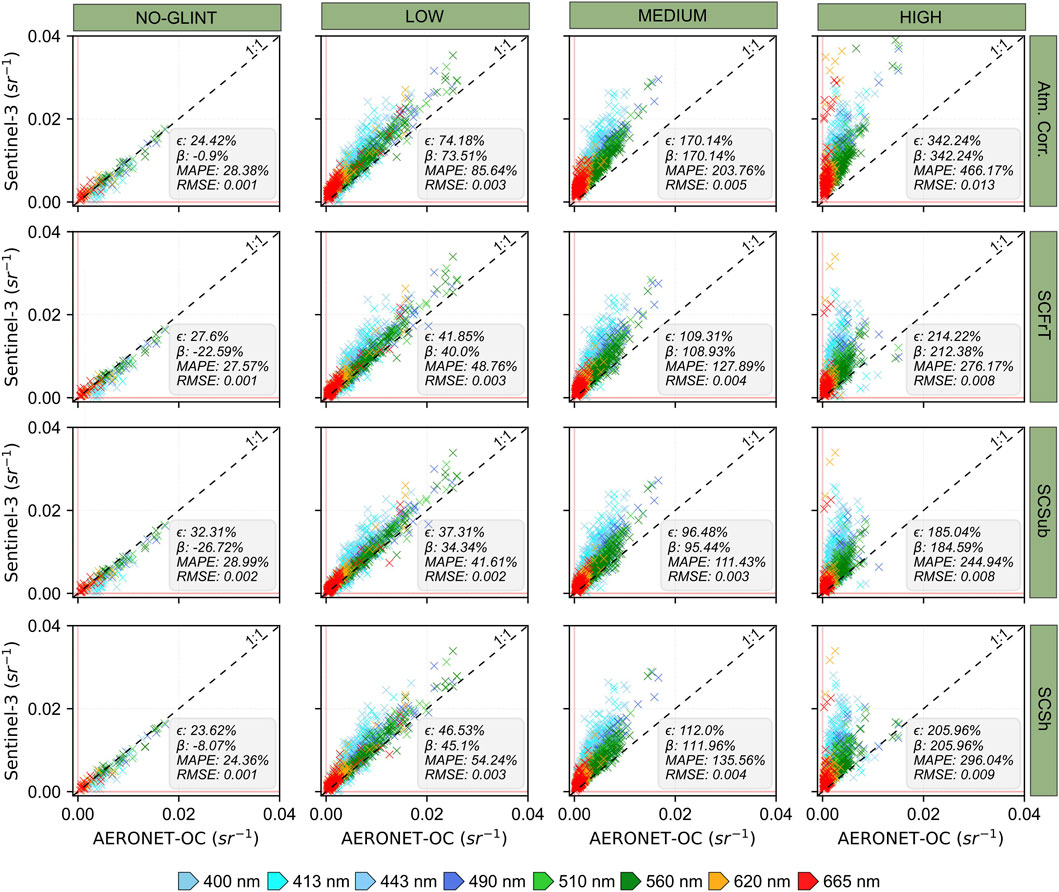
Figure 4. Validation of sunglint methods across various glint intensities. Colors represent the spectral bands (400, 413, 443, 490, 510, 560, 620, and 665 nm) in agreement between Sentinel-3 (A/B) OLCI and AERONET-OC. Failure data was not considered in this analysis (see Table A2, Supplementary Appendix A).

Blue wavelengths (400–490 nm) consistently showed higher errors across all correction methods in the presence of glint, highlighting the challenges in accurately retrieving aquatic reflectance values at shorter wavelengths using simple sunglint corrections. From low to high-glint conditions, the deglint methods showed slightly better agreement in longer wavelengths of the visible range (620 and 665 nm). However, under medium and high-glint intensities, all three algorithms significantly undercorrected R_rs values in wavelengths above 510 nm. Despite these limitations, significant improvements were observed in high-glint conditions when comparing corrected against uncorrected Sentinel-3 (A/B) OLCI data. On average, applied deglint methods reduced absolute errors by more than 128%, demonstrating their value in mitigating glint-induced distortions and enhancing the reliability of R_rs retrievals in glint-contaminated scenes.

Although the glint correction is essential for aquatic remote sensing applications, it involves certain tradeoffs due to occasional method failures (i.e., R_rs spectrum with negative values in any of the bands before or after glint corrections). To account for this factor in our analysis, we quantified the number of match-ups in which such failures occurred (Table A2, Supplementary Appendix A). Among the proposed algorithms, SCSh exhibited the highest number of failures (n = 48); however, this represented less than 9% of the total dataset (n = 570). These findings suggested that, overall, all three methods are generally effective in preventing invalid aquatic reflectance retrievals in Sentinel-3 (A/B) OLCI images across the visible spectral range (400–665 nm).

3.2 Insights from skyglint correction in the blue spectral range

The blue wavelengths (400–490 nm) from OLCI play a crucial role in estimating chlorophyll-a concentrations in the open ocean and CDOM in inland and coastal waters. However, our findings indicated that simple sunglint correction methods alone are not sufficient to achieve satisfactory performance within this range. To address this, we implemented a skyglint correction model (Gordon et al., 1988) in combination with sunglint corrections (Figure 5) to evaluate potential improvements. The inclusion of the skyglint component improved performance across low to high-glint intensities. Absolute errors were below 28% and 67% under low and medium-glint conditions, respectively. For high-glint, improvements were especially evident in the shorter wavelengths (400–560 nm); however, the accuracy remained insufficient to reliably support aquatic applications (ε > 100%). Notably, the blue wavelengths were better corrected with this approach. Conversely, under no-glint conditions, the combined correction performed poorly across all methods, with both ε and β above 53%, and a high incidence of overcorrection failures (Table A2, Supplementary Appendix A). Overall, SCSh + SkyG was the most conservative and reliable performance, showing the best balance between accuracy (Fig. A2; Supplementary Appendix A) and failure rate (Table A2; Supplementary Appendix A). While SCSub + SkyG also achieved low error values, it produced the highest number of failures (n = 137), indicating that this approach may lead to a significant number of invalid pixels in Sentinel-3 (A/B) OLCI images.

Figure 5

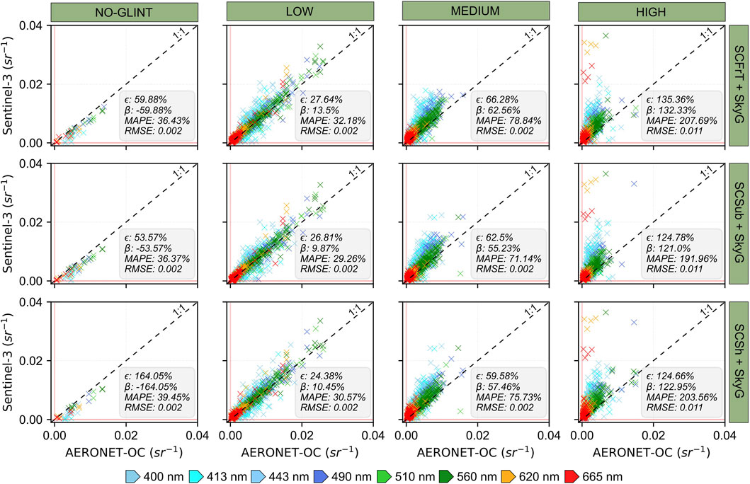
Figure 5. Validation of sunglint methods combined with SkyG across various glint intensities. Colors represent the spectral bands (400, 413, 443, 490, 510, 560, 620, and 665 nm) in agreement between Sentinel-3 (A/B) OLCI and AERONET-OC. Failure data was not considered in this analysis (see Table A2, Supplementary Appendix A).

Spectral similarities are shown in Figure 6. Notably, the blue wavelengths were better represented when skyglint correction was applied. These improvements were primarily observed as a reduction in spectral offset between Sentinel-3 (A/B) OLCI and AERONET-OC, with minor changes to the spectral shape. Low-glint conditions benefited the most from this approach, while medium and high-glint conditions still exhibited residual effects. By checking the AERONET-OC spectra under medium and high-glint, the R_rs values were less than 0.5%, making accurate retrieval particularly challenging under such conditions. Nevertheless, it is relevant to observe a reduction in spectral distortions even under these more extreme conditions. Although SCFrT + SkyG preserved the water spectrum in the valid match-ups (i.e., without failures) compared to other methods, all approaches – including this one – tended to compromise the shorter wavelengths (400–510 nm) when applied to pixels not affected by glint. This observation highlights the importance of using glint masks to guide correction strategies across the Sentinel-3 (A/B) OLCI images, ensuring that corrections are applied only where needed and avoiding unnecessary distortions in glint-free pixels.

Figure 6

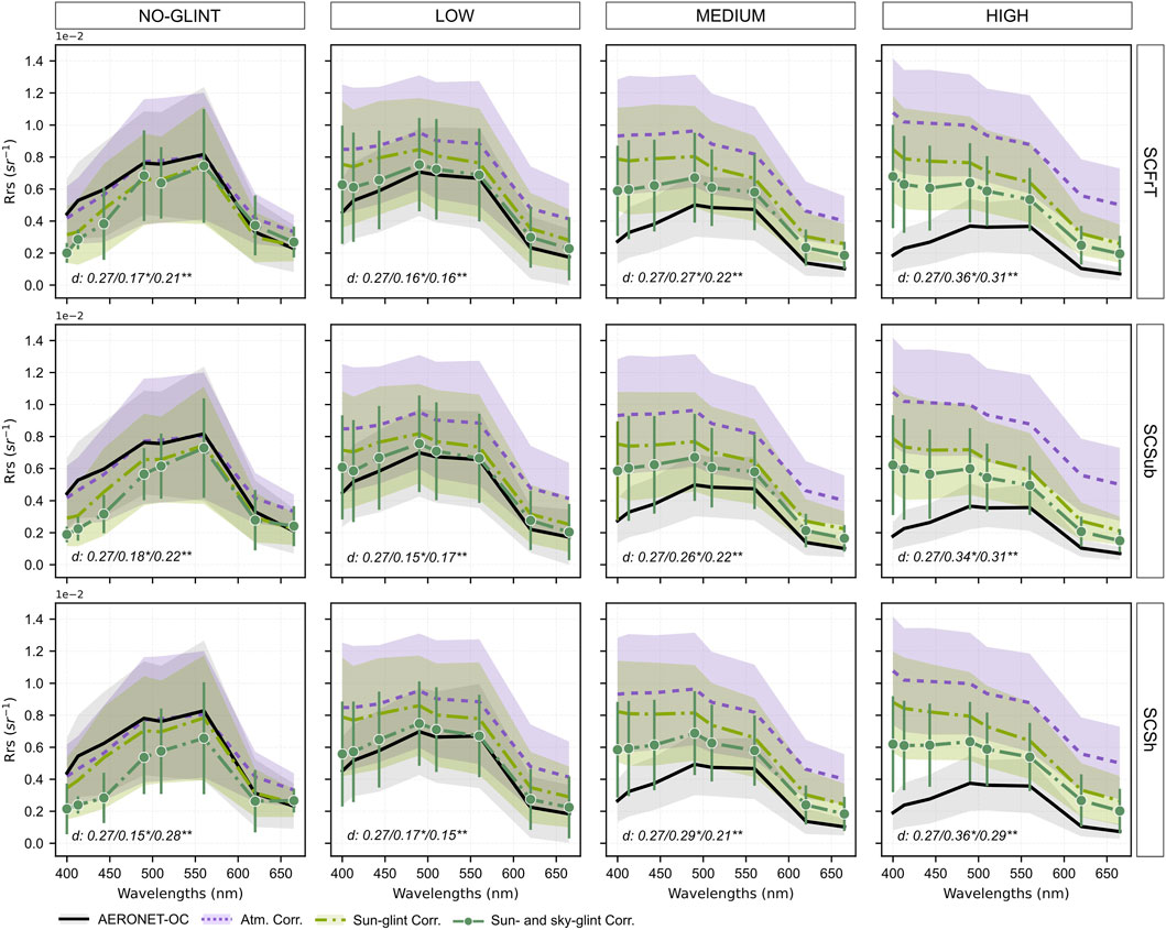
Figure 6. Spectral agreement between AERONET-OC and Sentinel-3 (A/B) OLCI R_rs after applying sunglint correction, as well as after combining sunglint and skyglint corrections. The data represent the mean and standard deviation within a percentile interval (5%–95%). The variable d indicates the average spectral similarity metric, with values marked by (*) and (**) representing those after the sunglint correction and combined sun and skyglint correction, respectively.

3.3 Analyzing the Sentinel-3 (A/B) OLCI image quality under visible glint conditions

The glint intensity classification used in this study (Section 2.5) revealed that when the glint is visible in 300 m Sentinel-3 (A/B) OLCI images, it typically corresponds to a medium- or high-level glint. After applying glint correction, a general reduction in image brightness is observed (Figure 7). To illustrate the performance of the different correction methods, we highlighted four representative cases (I–IV) where the effects of glint correction are clearly visible. Case I (SCFrT + SkyG (a)) shows residual glint effects after correction. Bright zones and glint-related textures remain visible, indicating that the correction method failed to fully remove glint. In Case II (SCSub + SkyG (a)), the corrected image demonstrates overcorrection, where zones previously affected by glint appear darker than their surroundings, suggesting an excessive correction of reflectance values. Case III (SCFrT + SkyG and SCSub + SkyG (c)) highlights overcorrection accompanied by artifact creation. In this case, some zones that were only slightly affected by glint in the original image appear unnaturally bright after correction, producing visual inconsistencies. Case IV (SCSh + SkyG (c)) showcases the benefits of effective glint correction. Previously hidden aquatic features, such as algal blooms, become visible after correction. In (b) and (d), all methods produced close brightness levels, but SCSh + SkyG was the most consistent approach across all examples. It visibly reduced glint while preventing artifacts, indicating that this method is more suitable under medium and high-glint conditions.

Figure 7

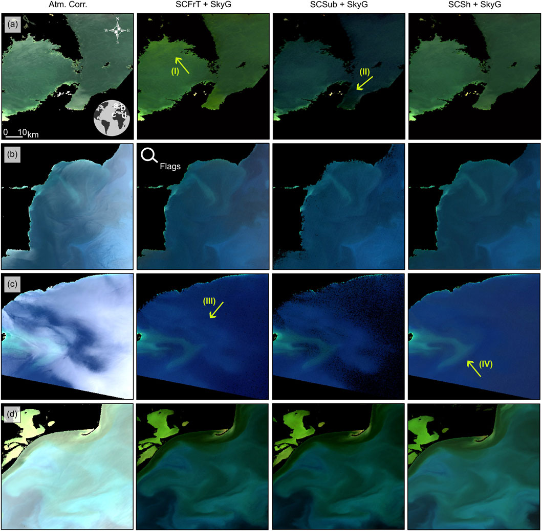
Figure 7. RGB (8-6-4) composite from Sentinel-3 A/B images showing instances where the glint effect is prominent before and after the correction. The narrows indicate specific cases observed post-correction: (I) represents residual glint effect that were not fully removed; (II) overcorrection resulting in dark areas in the images; (III) overcorrection with visual artefacts; and (IV) improved delineation of aquatic spectral features. All visualizations with similar local/date were adjusted using similar contrast and brightness levels to ensure a reliable comparison.

Figure 8 shows a comparison between two Sentinel-3 (A/B) OLCI images acquired on the same day. Panel (a) is strongly affected by glint, while panel (b) was captured under no-glint. In the absence of glint, both images are expected to yield comparable spectral responses over the same time and region. However, as shown in Figure 8f, the image with strong glint effects displays a significant spectral offset compared to both the no-glint and the AERONET-OC observations. Among all correction methods, only SCSh + SkyG (Figure 8e) successfully reduced the glint-induced spectral distortions, producing an R_rs spectrum that closely matches both the no-glint image and the AERONET-OC. The RGB composites (Figures 8c–e) highlight the differences in method performance. While all deglint methods reduced the visual impact of glint, only SCSh + SkyG provided a result visually consistent with the no-glint image reference (Figure 8b). In contrast, the other methods introduced visible overcorrections, suggesting that they may not be suitable for addressing extreme glint problems in Sentinel-3 (A/B) OLCI imagery.

Figure 8

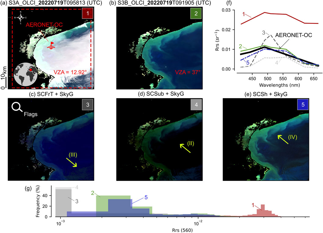
Figure 8. RGB (8-6-4) composite derived from Sentinel-3 OLCI images taken on the same day for sensors A (high-glint) and B (no-glint), as highlighted in plots (a,b) respectively. Additionally, composites from Sentinel-3A OLCI images following correction are presented (c–e) and the spectral agreement between the methods and images against AERONET-OC observation is examined (f,g). The numbers (1–5) in panels (f,g) correspond to the data derived from the images labeled accordingly.

3.4 Glint correction performance across OWTs

In this section, the spectral similarity between Sentinel-3 (A/B) OLCI and AERONET-OC observations is analyzed across various OWTs, ranging from low to high optical complexity (Figure 9). Overall, all three deglint methods (SCFrT, SCSub, and SCSh) demonstrated strong agreement with AERONET-OC, indicating that they are generally capable of preserving the spectral characteristics of different water types. Despite the application of both sun and skyglint corrections, a residual offset across the entire visible range was observed in waters with low optical complexity (Group A), with only minor disagreement in spectral shape (d < 0.15). As optical water complexity increased, the magnitude of spectral deviations also increased, particularly in the shorter wavelengths (400–510 nm), where the residual glint effect remained evident. Group E, representing the most optically complex waters, showed the largest discrepancies between Sentinel-3 (A/B) OLCI image and in situ spectra, with average d values exceeding 0.3. The failure analysis (Table A3, Supplementary Appendix A) revealed that most match-up failures occurred in waters with moderate optical complexity (Group C) (n > 73). Differently, waters in Groups A and E were least affected, with a failure count of less than two failures.

Figure 9

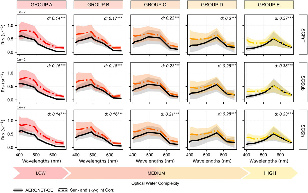
Figure 9. Spectral agreement between Sentinel-3 (A/B) OLCI after glint correction and AERONET-OC considering the different OWTs, ranging from low to high optical complexity (A-to-E groups). The data represent the mean and standard deviation within a percentile interval (5%–95%). The variable d indicates the average spectral similarity metric calculated between spectra.

4 Discussion

Our study assessed existing deglint methods for Sentinel-3 (A/B) OLCI imagery across varying glint intensities and optical water types. Among the proposed approaches, the combination of SCSh and SkyG achieved the best overall performance, with the lowest absolute error (ε < 58%) (Fig. A2, Supplementary Appendix A) and the fewest failure cases (n = 99, 17% of all match-ups) (Table A2, Supplementary Appendix A). This suggests that it is most effectively aligned with AERONET-OC observations while avoiding significant invalid values in the visible range (400–665 nm). Although SCFrT + SkyG and SCSub + SkyG exhibited errors close to SCSh (ε > 62.82%) (Fig. A2, Supplementary Appendix A), they frequently showed an elevated number of failures, approximately 21% (n = 120) and 24% (n = 137), respectively. No single method consistently performed well across all wavelengths and glint conditions, especially in the blue region (400–490 nm) and under the full range of glint intensities (i.e., No-Glint, Low, Medium, and High). While SCSub and SCFrT showed better results under low to medium-glint conditions, only SCSh could effectively minimize the glint effect in high-glint intensity (Figure 8). Achieving accurate aquatic reflectance is a challenge demonstrated in various studies (Maciel et al., 2023; Pahlevan et al., 2021; Vanhellemont and Ruddick, 2021; Warren et al., 2019), and our findings confirmed that glint miscorrection under high-glint conditions could introduce noticeable artifacts in 300 m Sentinel-3 (A/B) OLCI images (Figure 7). Under no-glint conditions, all evaluated methods tended to overcorrect the R_rs spectra. This outcome reinforces the necessity of applying glint masks (Wang and Bailey, 2001) to flag and exclude glint-free areas prior to correction, mainly when using coarser resolution images like Sentinel-3 (A/B) OLCI. All glint correction methods used need to be accompanied by a proper atmospheric correction (i.e., removal of atmospheric scattering and absorption contribution), which is inherently dependent on accurate atmospheric parameters such as aerosol optical thickness, aerosol type, and gaseous transmittance (Harmel et al., 2018). In the results presented, atmospheric correction was performed using on-ground-based products derived from AERONET to ensure high consistency across matchups and to minimize residual atmospheric effects. Unfortunately, AERONET is not dense enough to provide data for all aquatic systems. In such cases, other sources can be used to derive atmospheric parameters, such as those offered by MODIS and VIIRS (Caballero et al., 2025), noting that the global accuracy remains dependent on the quality and regional representativeness of these products.

Including skyglint correction (SkyG) significantly improved the retrievals in the blue wavelengths (Figure 5). Across all glint-intensity categories, reflectance in the blue wavelengths was reduced, bringing the values into closer agreement with AERONET-OC observations. The combination of sunglint methods with SkyG reduced R_rs by nearly threefold (∼65%) relative to the uncorrected values (Fig. A1 and Fig. A2, Supplementary Appendix A), yielding the most accurate results under low to medium-glint conditions, which were the best-resolved scenarios in this study. Even under high-glint conditions, some improvements were observed in the shorter wavelengths, although the overall accuracy remained insufficient for aquatic applications (ε > 100%). These applications typically require error rates to meet the accurate retrieval of OACs in ocean color products (<30%) (Global Climate Observing System, 2016). When considering optical water types (Figure 9), no significant difference was observed between deglint method performance, which means all methods preserved spectral water features. However, waters with higher optical complexity exhibited more pronounced spectral distortions than those with lower optical complexity. The shorter wavelengths (400–510 nm) remained particularly challenging, as their spectral shapes often deviated from those observed in AERONET-OC spectra. This may be due to a residual skyglint effect that is observable under medium and high-glint intensity (Figure 5). Furthermore, the absorption features caused by overlapping phytoplankton and colored dissolved organic matter (CDOM) lead to very low R_rs values in this range (Liu et al., 2021; Song et al., 2015; Zhang et al., 2021), making spectral agreement between Sentinel-3 (A/B) OLCI and AERONET-OC especially difficult to achieve.

All deglint methods tested in this study showed limitations within our processing scheme. A critical challenge in sunglint correction is the dependence on wavelength-specific assumptions. The SCFrT and SCSub methods infer sunglint intensity based on a longer wavelength signal (Vanhellemont, 2019). For Sentinel-3 (A/B) OLCI, we adopted the spectral band centered at 1,020 nm as a reference because it is the longest wavelength available and the most spectrally distant from the visible domain. However, in optically clear waters, atmospheric correction at this spectral range can yield negative reflectance values due to its low signal-to-noise ratio (reference SNR ∼152; Donlon et al., 2012), whereas in shallow or turbid waters, residual water-leaving reflectance can persist beyond 900 nm (Ruddick et al., 2000; Wang et al., 2012). This behavior indicates that the 1,020 nm band cannot always be considered a perfectly dark reference, which may contribute to overcorrection or instability in the SCFrT and SCSub outputs. In our analysis, the spectral behavior remained consistent across glint levels (Figures 6, 9), and no anomalous patterns were observed that would indicate significant contamination by nonzero reflectance at 1,020 nm. These findings suggest that while the use of 1,020 nm introduces potential uncertainty in shallow or highly turbid environments, it provides a practical proxy for glint estimation within the range of conditions analyzed in this study.

The SCSh method offers a reliable alternative for clear and moderately turbid waters by using the oxygen absorption band centered at 761 nm (Kutser et al., 2009). However, because this wavelength lies within the atmospheric oxygen absorption region, uncertainties in gaseous transmittance could bias the inferred glint magnitude, especially over no-glint conditions, as suggested by Kutser et al., 2009. Under this condition, the glint signal is negligible compared to the uncertainties associated with the atmospheric transmission, making the method more sensitive to minor deviations in the 761 wavelengths. Conversely, when glint is present, its contribution to the total radiance dominates these minor uncertainties, reducing their relative influence on the correction accuracy. Similar to the limitations faced with SCFrT and SCSub, obtaining a pure sunglint signal at this wavelength, free from the influence of OACs, can be particularly challenging in highly turbid waters. High concentrations of particles like suspended sediments or phytoplankton tend to scatter light at longer wavelengths (Kirk, 2011), complicating the isolation of pure glint signals. Additionally, this method assumes a variable sunglint intensity across the image and spatially homogeneous water properties, which is not always the case. The methods used implicitly assume a linear relationship between the glint intensity observed in the reference and visible bands, which in reality can vary with atmospheric properties (Kay et al., 2009). The simplification of addressing sunglint solely through spectral relationships also poses intrinsic limitations, since glint intensity is influenced by external factors such as geometry and surface roughness (Cox and Munk, 1954). In Sentinel-3 (A/B) OLCI imagery, these limitations can be particularly critical because the sensor’s wide swath (1,270 km) results in variations in illumination-viewing geometry across the scene (D’Alimonte et al., 2025). As a consequence, glint intensity can vary markedly within the same acquisition, and this partially explains the reduced performance of all tested methods under high-glint conditions.

Another challenge relates to the application of skyglint correction. While we intended to enhance the glint removal in Sentinel-3 (A/B) OLCI images, combining both corrections (sunglint + skyglint) often led to negative R_rs values (>620 nm), resulting in the complete loss of affected pixels (Table A2, Supplementary Appendix A). As such, skyglint correction is best recommended when shorter wavelengths are the primary focus in aquatic applications. For example, conventional bio-optical algorithms dedicated to open ocean waters estimate chlorophyll-a, an algal pigment used as a proxy for primary productivity (Matthews, 2017), relying on blue-green ratios (443/490 nm–560 nm) (O’Reilly et al., 1998). Also, inland and coastal waters may use these wavelengths to estimate CDOM (e.g., 412, 443, and 490 nm) (Bonelli et al., 2021; Huang et al., 2022) and the Secchi depth (e.g., 490 nm) (Maciel et al., 2023).

Sentinel-3 (A/B) OLCI is a key ocean color sensor that has provided nearly a decade of high-quality multispectral data critical for aquatic studies. Given its proven performance, there is a significant opportunity for synergistic use of Sentinel-3 (A/B) OLCI with other satellites (Pahlevan et al., 2020; Warren et al., 2021), including the new generation of hyperspectral sensors dedicated to aquatic investigations, such as NASA’s PACE (Plankton, Aerosol, Cloud, and Ocean Ecosystem) mission (launched on 8 February 2024) (Werdell et al., 2019). Its use in developing synthetic images with super-resolution is also requested (Paulino et al., 2025). This demands increasingly robust data processing, including glint correction. Although Sentinel-3 (A/B) OLCI includes mechanisms to mitigate glint (Donlon et al., 2012), our analysis showed that this problem is still prevalent, with 97% of our dataset affected to some degree. This highlighted the need for reliable deglint solutions. In addition to traditional correction approaches, emerging machine learning and deep learning techniques show considerable potential – whether applied to atmospheric correction (Zhao et al., 2023) or designed explicitly for glint removal (Giles et al., 2021) – and may help overcome limitations observed in current methods. Therefore, ongoing improvements in processing deglint methodologies for Sentinel-3 OLCI are essential to ensure accurate, consistent, and long-term monitoring of aquatic systems.

5 Conclusion

This study demonstrated that glint – both sun and skyglint effects – constituents a significant challenge in imagery acquired by Sentinel-3 (A/B) OLCI. We evaluated three methodologies for removing these effects, and overall, all image-based sunglint methods, when combined with skyglint correction, produced improvements in Sentinel-3 (A/B) OLCI imagery. Among them, the combination of SCSh (i.e., a sunglint removal method designed for optically shallow waters) and SkyG (i.e., an analytical skyglint removal method) emerged as the most reliable, effectively reducing spectral distortions while preserving aquatic features across varying glint intensities and optical water types. Conversely, no single method worked perfectly in all glint contexts. The blue spectral bands (400–490 nm) were particularly susceptible to miscorrections, and in glint-free conditions, all applied methods tended to overcorrect R_rs values. This reinforces the critical role of glint detection and its masking in image preprocessing workflows. While no universal solution exists for correcting glint effects across varying intensities, it became evident that the implementation of glint correction substantially enhances the quality of Sentinel-3 (A/B) OLCI imagery. Moving forward, future efforts should focus on improving the spectral consistency of Sentinel-3 (A/B) OLCI images under medium and high-glint conditions, particularly within the blue wavelengths. Advancements in glint correction are vital for unlocking the full potential of Sentinel-3 (A/B) OLCI imagery for inland, coastal, and oceanic water quality monitoring applications.

Data availability statement

The raw data supporting the conclusions of this article will be made available by the authors, without undue reservation.

Author contributions

RSP: Conceptualization, Formal Analysis, Methodology, Software, Writing – original draft. VSM: Conceptualization, Methodology, Writing – review and editing. CBC: Writing – review and editing. TMAL: Writing – review and editing. DAM: Writing – review and editing. JCPS: Writing – review and editing. BL: Writing – review and editing.

Funding

The authors declare that financial support was received for the research and/or publication of this article. We thank the European Space Agency for providing the images used in this study. We also thank the AERONET-OC PIs (Barbara Bulgarelli, Robert Frouin, Pawan Gupta, Susanne Kratzer, Hubert Loisel, Frederic Melin, Paula Pratolongo, Dimitry Van der Zande, Giuseppe Zibordi) for their efforts in establishing and maintaining AERONET-OC sites. Martins thanks the support of grants #80NSSC24K1040 awarded by NASA Early Career Investigator Program in Earth Science, and #8007148-04.01 awarded by Mississippi Based RESTORE Act Center of Excellence (MBRACE) program. This project was paid for with federal funding from the U.S. Department of the Treasury, the Mississippi Department of Environmental Quality, and the Mississippi Based RESTORE Act Center of Excellence under the Resources and Ecosystems Sustainability, Tourist Opportunities, and Revived Economies of the Gulf Coast States Act of 2012 (RESTORE Act). The statements, findings, conclusions, and recommendations are those of the author(s) and do not necessarily reflect the views of the Department of the Treasury, the Mississippi Department of Environmental Quality, or the Mississippi Based RESTORE Act Center of Excellence.

Conflict of interest

The authors declare that the research was conducted in the absence of any commercial or financial relationships that could be construed as a potential conflict of interest.

The handling editor ZC declared past co-authorship with the author DAM.

Generative AI statement

The authors declare that Generative AI was used in the creation of this manuscript. During the preparation of this work, the author(s) used Grammarly and ChatGPT in order to improve grammar and text flow. After using this tool/service, the author(s) reviewed and edited the content as needed and take full responsibility for the publication’s content.

Any alternative text (alt text) provided alongside figures in this article has been generated by Frontiers with the support of artificial intelligence and reasonable efforts have been made to ensure accuracy, including review by the authors wherever possible. If you identify any issues, please contact us.

Publisher’s note

All claims expressed in this article are solely those of the authors and do not necessarily represent those of their affiliated organizations, or those of the publisher, the editors and the reviewers. Any product that may be evaluated in this article, or claim that may be made by its manufacturer, is not guaranteed or endorsed by the publisher.

Supplementary material

The Supplementary Material for this article can be found online at: https://www.frontiersin.org/articles/10.3389/frsen.2025.1690337/full#supplementary-material

References

Baker, K. S., and Smith, R. C. (1982). Bio-optical classification and model of natural waters. 21. Limnol. Oceanogr. 27, 500–509. doi:10.4319/lo.1982.27.3.0500

CrossRef Full Text | Google Scholar

Bassani, C., Cazzaniga, I., Manzo, C., Bresciani, M., Braga, F., Giardino, C., et al. (2016). Atmospheric and adjacency correction of Landsat-8 imagery of inland and coastal waters near AERONET-OC sites, 740, 259.

Google Scholar

Begliomini, F. N., Barbosa, C. C., Martins, V. S., Novo, E. M., Paulino, R. S., Maciel, D. A., et al. (2023). Machine learning for Cyanobacteria mapping on tropical urban reservoirs using PRISMA hyperspectral data. ISPRS J. Photogrammetry Remote Sens. 204, 378–396. doi:10.1016/j.isprsjprs.2023.09.019

CrossRef Full Text | Google Scholar

Bonelli, A. G., Vantrepotte, V., Jorge, D. S. F., Demaria, J., Jamet, C., Dessailly, D., et al. (2021). Colored dissolved organic matter absorption at global scale from ocean color radiometry observation: spatio-temporal variability and contribution to the absorption budget. Remote Sens. Environ. 265, 112637. doi:10.1016/j.rse.2021.112637

CrossRef Full Text | Google Scholar

Bréon, F. M., and Henriot, N. (2006). Spaceborne observations of ocean glint reflectance and modeling of wave slope distributions. J. Geophys. Res. Oceans 111. doi:10.1029/2005JC003343

CrossRef Full Text | Google Scholar

Bulgarelli, B., and Zibordi, G. (2018). On the detectability of adjacency effects in ocean color remote sensing of mid-latitude coastal environments by SeaWiFS, MODIS-A, MERIS, OLCI, OLI and MSI. Remote Sens. Environ. 209, 423–438. doi:10.1016/j.rse.2017.12.021

PubMed Abstract | CrossRef Full Text | Google Scholar

Bulgarelli, B., Kiselev, V., and Zibordi, G. (2014). Simulation and analysis of adjacency effects in coastal waters: a case study. A Case Study 53, 1523–1545. doi:10.1364/ao.53.001523

PubMed Abstract | CrossRef Full Text | Google Scholar

Caballero, C. B., Martins, V. S., Paulino, R. S., Lima, T. M., Butler, E., and Sparks, E. (2025). Sentinel-3 coastal analysis ready data (S3CARD): an operational framework for coastal water applications. Water Res. 287, 124432. doi:10.1016/j.watres.2025.124432

PubMed Abstract | CrossRef Full Text | Google Scholar

Chen, J., He, X., Liu, Z., Lin, N., Xing, Q., and Pan, D. (2021). Sun glint correction with an inherent optical properties data processing system. Int. J. Remote Sens. 42, 617–638. doi:10.1080/01431161.2020.1811916

CrossRef Full Text | Google Scholar

Cox, C., and Munk, W. (1954). Statistics of the sea surface derived from sun glitter. J. Mar. Res. 198–227.

Google Scholar

Cox, C., and Munk, W. (1955). Slopes of the sea surface deduced from photographs of sun glitter. Bulletin of the Scripps Institution of Oceanography of the University of California. 6 (9). 401–487.

Google Scholar

de Lima, T. M., Barbosa, C. C., Nordi, C. S., Begliomini, F. N., Martins, V. S., Watanabe, F. S., et al. (2025). A novel hybrid Cyanobacteria mapping approach for inland reservoirs using Sentinel-3 imagery. Harmful Algae 144, 102836. doi:10.1016/j.hal.2025.102836

PubMed Abstract | CrossRef Full Text | Google Scholar

Dierssen, H. M., Ackleson, S. G., Joyce, K. E., Hestir, E. L., Castagna, A., Lavender, S., et al. (2021). Living up to the hype of hyperspectral aquatic remote sensing: science, resources and outlook. Resour. Outlook 9, 649528. doi:10.3389/fenvs.2021.649528

CrossRef Full Text | Google Scholar

Donlon, C., Berruti, B., Buongiorno, A., Ferreira, M. H., F´em´enias, P., Frerick, J., et al. (2012). The global monitoring for environment and security (GMES) Sentinel-3 mission. Remote Sens. Environ. 120, 37–57. doi:10.1016/j.rse.2011.07.024

CrossRef Full Text | Google Scholar

D’Alimonte, D., Kajiyama, T., Pitarch, J., Brando, V. E., Talone, M., Mazeran, C., et al. (2025). Comparison of correction methods for bidirectional effects in ocean colour remote sensing. Remote Sens. Environ. 321, 114606. doi:10.1016/j.rse.2025.114606

CrossRef Full Text | Google Scholar

Eck, T. F., Holben, B. N., Reid, J. S., Dubovik, O., Smirnov, A., O’Neill, N. T., et al. (1999). Wavelength dependence of the optical depth of biomass burning, urban, and desert dust aerosols. J. Geophys. Res. Atmos. 104, 31333–31349. doi:10.1029/1999JD900923

CrossRef Full Text | Google Scholar

Feng, L., and Hu, C. (2016). Cloud adjacency effects on top-of-atmosphere radiance and ocean color data products: a statistical assessment. Remote Sens. Environ. 174, 301–313. doi:10.1016/j.rse.2015.12.020

CrossRef Full Text | Google Scholar

Frouin, R., Schwindling, M., and Deschamps, P. Y. (1996). Spectral reflectance of sea foam in the visible and near-infrared: in situ measurements and remote sensing implications. J. Geophys. Res. Oceans 101, 14361–14371. doi:10.1029/96JC00629

CrossRef Full Text | Google Scholar

Fukushima, H., Suzuki, K., Li, L., Suzuki, N., and Murakami, H. (2009). Improvement of the ADEOS-II/GLI sun-glint algorithm using concomitant microwave scatterometer-derived wind data. Adv. Space Res. 43, 941–947. doi:10.1016/j.asr.2008.07.013

CrossRef Full Text | Google Scholar

Giles, A. B., Davies, J. E., Ren, K., and Kelaher, B. (2021). A deep learning algorithm to detect and classify sun glint from high-resolution aerial imagery over shallow marine environments. ISPRS J. Photogrammetry Remote Sens. 181, 20–26. doi:10.1016/j.isprsjprs.2021.09.004

CrossRef Full Text | Google Scholar

Global Climate Observing System (GCOS) (2016). The global observing system for climate: implementation needs. Available online at: https://gcos.wmo.int/site/global-climate-observing-system-gcos/publications (Accessed in July 2025).

Google Scholar

Goodman, J. A., Lee, Z., and Ustin, S. L. (2008). Influence of atmospheric and sea-surface corrections on retrieval of bottom depth and reflectance using a semi-analytical model: a case study in kaneohe Bay, Hawaii. Appl. Opt. 47, F1–F11. doi:10.1364/ao.47.0000f1

PubMed Abstract | CrossRef Full Text | Google Scholar

Gordon, H. R. (1997). Atmospheric correction of ocean color imagery in the Earth observing system era. J. Geophys. Res. Atmos. 102, 17081–17106. doi:10.1029/96jd02443

CrossRef Full Text | Google Scholar

Gordon, H. R. (2021). Evolution of ocean color atmospheric correction: 1970–2005. Remote Sens. 13, 5051–2005. doi:10.3390/rs13245051

CrossRef Full Text | Google Scholar

Gordon, H. R., and Wang, M. (1994a). Retrieval of water-leaving radiance and aerosol optical thickness over the oceans with SeaWiFS: a preliminary algorithm. Appl. Opt. 33, 443. doi:10.1364/ao.33.000443

PubMed Abstract | CrossRef Full Text | Google Scholar

Gordon, H. R., and Wang, M. (1994b). Influence of Oceanic whitecaps on atmospheric correction of ocean-color sensors. Appl. Opt. 33, 7754. doi:10.1364/AO.33.007754

PubMed Abstract | CrossRef Full Text | Google Scholar

Gordon, H. R., Brown, J. W., and Evans, R. H. (1988). Exact rayleigh scattering calculations for use with the nimbus-7 coastal zone color scanner. Tech. Rep. 27, 862. doi:10.1364/ao.27.000862

PubMed Abstract | CrossRef Full Text | Google Scholar

Harmel, T., Chami, M., Tormos, T., Reynaud, N., and Danis, P. A. (2018). Sunglint correction of the multi-spectral instrument (MSI)-SENTINEL-2 imagery over inland and sea waters from SWIR bands. Remote Sens. Environ. 204, 308–321. doi:10.1016/j.rse.2017.10.022

CrossRef Full Text | Google Scholar

Hedley, J. D., Harborne, A. R., and Mumby, P. J. (2005). Technical note: simple and robust removal of sun glint for mapping shallow-water benthos. Int. J. Remote Sens. 26, 2107–2112. doi:10.1080/01431160500034086

CrossRef Full Text | Google Scholar

Huang, J., Chen, J., Wu, M., Gong, L., and Zhang, X. (2022). Estimation of chromophoric dissolved organic matter and its controlling factors in beaufort sea using mixture density network and Sentinel-3 data. Sci. Total Environ. 849, 157677. doi:10.1016/j.scitotenv.2022.157677

PubMed Abstract | CrossRef Full Text | Google Scholar

Kay, S., Hedley, J. D., and Lavender, S. (2009). Sun glint correction of high and low spatial resolution images of aquatic scenes: a review of methods for visible and near-infrared wavelengths. Remote Sens. 1, 697–730. doi:10.3390/rs1040697

CrossRef Full Text | Google Scholar

Kirk (2011). Light and photosynthesis in aquatic ecosystems.

Google Scholar

Kotchenova, S. Y., Vermote, E. F., Matarrese, R., and Klemm, F. J. (2006). Validation of a vector version of the 6S radiative transfer code for atmospheric correction of satellite data. Part I: path radiance. Tech. Rep. 45, 6762. doi:10.1364/ao.45.006762

PubMed Abstract | CrossRef Full Text | Google Scholar

Kruse, F. A., Lefkoff, A. B., Boardman, J. W., Heidebrecht, K. B., Shapiro, A. T., Barloon, P. J., et al. (1993). The spectral image processing system (SIPS) interactive visualization and analysis of imaging spectrometer data, 163, 145–163.

CrossRef Full Text | Google Scholar

Kutser, T., Vahtmäe, E., and Praks, J. (2009). Remote sensing of environment A sun glint correction method for hyperspectral imagery containing areas with non-negligible water leaving NIR signal. Remote Sens. Environ. 113, 2267–2274. doi:10.1016/j.rse.2009.06.016

CrossRef Full Text | Google Scholar

Liu, B., D’Sa, E. J., Maiti, K., Rivera-Monroy, V. H., and Xue, Z. (2021). Biogeographical trends in phytoplankton community size structure using adaptive sentinel 3-OLCI chlorophyll a and spectral empirical orthogonal functions in the estuarine-shelf waters of the northern Gulf of Mexico. Remote Sens. Environ. 252, 112154. doi:10.1016/j.rse.2020.112154

CrossRef Full Text | Google Scholar

Lloyd, S. P. (1982). Least squares quantization in PCM. IEEE Trans. Inf. Theory 28, 129–137. doi:10.1109/tit.1982.1056489

CrossRef Full Text | Google Scholar

Lobo, F. L., Costa, M. P. F., and Novo, E. M. L. M. (2014). Time-series analysis of Landsat-MSS/TM/OLI images over Amazonian waters impacted by gold mining activities. Remote Sens. Environ. 157, 170–184. doi:10.1016/j.rse.2014.04.030

CrossRef Full Text | Google Scholar

Maciel, D. A., Barbosa, C. C. F., Novo, E. M. L. d.M., Flores Junior, R., and Begliomini, F. N. (2021). Water clarity in Brazilian water assessed using Sentinel-2 and machine learning methods. ISPRS J. Photogrammetry Remote Sens. 182, 134–152. doi:10.1016/j.isprsjprs.2021.10.009

CrossRef Full Text | Google Scholar

Maciel, D. A., Pahlevan, N., Barbosa, C. C., Martins, V. S., Smith, B., O’Shea, R. E., et al. (2023). Towards global long-term water transparency products from the landsat archive. Remote Sens. Environ. 299, 113889. doi:10.1016/j.rse.2023.113889

CrossRef Full Text | Google Scholar

Matthews, M. W. (2017). “Bio-optical modeling of phytoplankton Chlorophyll-a,” in Bio-optical modeling and remote sensing of inland waters (Elsevier Inc.), 157–188. doi:10.1016/B978-0-12-804644-9.00006-9

CrossRef Full Text | Google Scholar

Mélin, F. (2022). Validation of ocean color remote sensing reflectance data: analysis of results at European coastal sites. Remote Sens. Environ. 280, 113153. doi:10.1016/j.rse.2022.113153

CrossRef Full Text | Google Scholar

Mishra, S., Stumpf, R. P., Schaeffer, B. A., Werdell, P. J., Loftin, K. A., and Meredith, A. (2019). Measurement of cyanobacterial bloom magnitude using satellite remote sensing. Sci. Rep. 9, 18310–18317. doi:10.1038/s41598-019-54453-y

PubMed Abstract | CrossRef Full Text | Google Scholar

Mobley, C. D. (2015). Polarized reflectance and transmittance properties of windblown sea surfaces. Appl. Opt. 54, 4828. doi:10.1364/ao.54.004828

PubMed Abstract | CrossRef Full Text | Google Scholar

Moore, T. S., Dowell, M. D., Bradt, S., and Ruiz Verdu, A. (2014). An optical water type framework for selecting and blending retrievals from bio-optical algorithms in lakes and coastal waters. Remote Sens. Environ. 143, 97–111. doi:10.1016/j.rse.2013.11.021

PubMed Abstract | CrossRef Full Text | Google Scholar

Morel, A., and Prieur, L. (1977). Analysis of variations in ocean color. Limnol. Oceanogr. 22, 709–722. doi:10.4319/lo.1977.22.4.0709

CrossRef Full Text | Google Scholar

Morley, S. K. (2016). Alternatives to accuracy and bias metrics based on percentage errors for radiation belt modeling applications intended for: alternatives to accuracy and bias metrics based on percentage errors for radiation belt modeling applications. doi:10.2172/1260362

CrossRef Full Text | Google Scholar

Morley, S. K., Brito, T. V., and Welling, D. T. (2018). Measures of model performance based on the log accuracy ratio. Space weather. 16, 69–88. doi:10.1002/2017SW001669

CrossRef Full Text | Google Scholar

Mueller, J. L., and Austin, R. W. (1995). Ocean optics protocols for SeaWiFS validation, revision 1, SeaWiFS technical report series in NASA tech. Memo. 104566. Editors S. B. Hooker, E. R. Firestone, and J. G. Acker (Springfield, Va: National Technical Information Service), 25.

Google Scholar

O’Reilly, J. E., Maritorena, S., Mitchell, B. G., Siegel, D. A., Carder, K. L., Garver, S. A., et al. (1998). Ocean color chlorophyll algorithms for SeaWiFS. J. Geophys. Res. Oceans 103, 24937–24953. doi:10.1029/98JC02160

CrossRef Full Text | Google Scholar

Pahlevan, N., Smith, B., Schalles, J., Binding, C., Cao, Z., Ma, R., et al. (2020). Seamless retrievals of chlorophyll-a from Sentinel-2 (MSI) and Sentinel-3 (OLCI) in inland and coastal waters: a machine-learning approach. Remote Sens. Environ. 240, 111604. doi:10.1016/j.rse.2019.111604

CrossRef Full Text | Google Scholar

Pahlevan, N., Mangin, A., Balasubramanian, S. V., Smith, B., Alikas, K., Arai, K., et al. (2021). ACIX-Aqua: a global assessment of atmospheric correction methods for Landsat-8 and Sentinel-2 over Lakes, rivers, and coastal waters. Remote Sens. Environ. 258, 112366. doi:10.1016/j.rse.2021.112366

CrossRef Full Text | Google Scholar

Paulino, R. S., Martins, V. S., Novo, E. M. L. M., Barbosa, C. C. F., Carvalho, L. A. S. D., and Begliomini, F. N. (2022). Assessment of adjacency correction over inland waters using Sentinel-2 MSI images. Remote Sens. (Basel). 14, 1829. doi:10.3390/rs14081829

CrossRef Full Text | Google Scholar

Paulino, R., Martins, V., Caballero, C., Lima, T., Liu, B., and Ashapurec, A. (2026). PACE (plankton, aerosol, Cloud, ocean ecosystem): preliminary analysis of the consistency of remote sensing reflectance product over aquatic systems. ISPRS J. Photogrammetry Remote Sens.

Google Scholar

Paulino, R. S., Martins, V. S., Novo, E. M. L. M., Barbosa, C. C. F., Maciel, D. A., Do, R. L., et al. (2025). Generation of robust 10-m Sentinel-2/3 synthetic aquatic reflectance bands over inland waters. Remote Sens. Environ. 318, 114593. doi:10.1016/j.rse.2024.114593

CrossRef Full Text | Google Scholar

Ruddick, K. G., Ovidio, F., and Rijkeboer, M. (2000). Atmospheric correction of SeaWiFS imagery for turbid coastal and inland waters. Tech. Rep. 39, 897. doi:10.1364/ao.39.000897

PubMed Abstract | CrossRef Full Text | Google Scholar

Schaeffer, B. A., Reynolds, N., Ferriby, H., Salls, W., Smith, D., Johnston, J. M., et al. (2024). Forecasting freshwater cyanobacterial harmful algal blooms for Sentinel-3 satellite resolved U.S. Lakes and reservoirs. J. Environ. Manag. 349, 119518. doi:10.1016/j.jenvman.2023.119518

PubMed Abstract | CrossRef Full Text | Google Scholar

Shen, M., Duan, H., Cao, Z., Xue, K., Qi, T., Ma, J., et al. (2020). Sentinel-3 OLCI observations of water clarity in large Lakes in eastern China: implications for SDG 6.3.2 evaluation. Remote Sens. Environ. 247, 111950. doi:10.1016/j.rse.2020.111950

CrossRef Full Text | Google Scholar

Song, K., Li, L., Tedesco, L., Clercin, N., Li, L., and Shi, K. (2015). Spectral characterization of colored dissolved organic matter for productive inland waters and its source analysis. Chin. Geogr. Sci. 25, 295–308. doi:10.1007/s11769-014-0690-5

CrossRef Full Text | Google Scholar

Spyrakos, E., O’Donnell, R., Hunter, P. D., Miller, C., Scott, M., Simis, S. G., et al. (2018). Optical types of inland and coastal waters. Limnol. Oceanogr. 63, 846–870. doi:10.1002/lno.10674

CrossRef Full Text | Google Scholar

Vanhellemont, Q. (2019). Adaptation of the dark spectrum fitting atmospheric correction for aquatic applications of the landsat and Sentinel-2 archives. Remote Sens. Environ. 225, 175–192. doi:10.1016/j.rse.2019.03.010

CrossRef Full Text | Google Scholar

Vanhellemont, Q., and Ruddick, K. (2018). Atmospheric correction of metre-scale optical satellite data for inland and coastal water applications. Remote Sens. Environ. 216, 586–597. doi:10.1016/j.rse.2018.07.015

CrossRef Full Text | Google Scholar

Vanhellemont, Q., and Ruddick, K. (2021). Atmospheric correction of Sentinel-3/OLCI data for mapping of suspended particulate matter and chlorophyll-a concentration in Belgian turbid coastal waters. Remote Sens. Environ. 256, 112284. doi:10.1016/j.rse.2021.112284

CrossRef Full Text | Google Scholar

Vermote, E., Tanre, D., Deuze, J. L., Herman, M., and Santer, R. (1997). Second simulation of the satellite signal in the solar spectrum, 6S: an overview. IEEE Trans. GEOSCIENCE REMOTE Sens. 35, 187. doi:10.1109/igarss.1990.688308

CrossRef Full Text | Google Scholar

Vermote, E., Tanré, D., Deuz´e, J. L., and Herman, M. (2006). Simulation of the Satellite Signal in the Solar Spectrum (6S), 6S User Guide Version 3.0. Greenbelt, MD: NASA-GSFC.

Google Scholar

Wang, M., and Bailey, S. W. (2001). Correction of sun glint contamination on the SeaWiFS ocean and atmosphere products. Tech. Rep. doi:10.1364/ao.40.004790

PubMed Abstract | CrossRef Full Text | Google Scholar

Wang, M., and Shi, W. (2007). The NIR-SWIR combined atmospheric correction approach for MODIS ocean color data processing. Opt. EXPRESS 15, 15722–12. doi:10.1364/oe.15.015722

PubMed Abstract | CrossRef Full Text | Google Scholar

Wang, M., Shi, W., and Jiang, L. (2012). Atmospheric correction using near-infrared bands for satellite ocean color data processing in the turbid Western Pacific region. Opt. Express 20, 741. doi:10.1364/oe.20.000741

PubMed Abstract | CrossRef Full Text | Google Scholar

Warren, M. A., Simis, S. G., Martinez-Vicente, V., Poser, K., Bresciani, M., Alikas, K., et al. (2019). Assessment of atmospheric correction algorithms for the Sentinel-2A MultiSpectral imager over coastal and inland waters. Remote Sens. Environ. 225, 267–289. doi:10.1016/j.rse.2019.03.018

CrossRef Full Text | Google Scholar

Warren, M. A., Simis, S. G. H., and Selmes, N. (2021). Complementary water quality observations from high and medium resolution sentinel sensors by aligning chlorophyll-a and turbidity algorithms. Remote Sens. Environ. 265, 112651. doi:10.1016/j.rse.2021.112651

PubMed Abstract | CrossRef Full Text | Google Scholar

Wei, J., Wang, M., Mikelsons, K., Jiang, L., Kratzer, S., Lee, Z., et al. (2022). Global satellite water classification data products over Oceanic, coastal, and inland waters. Remote Sens. Environ. 282, 113233. doi:10.1016/j.rse.2022.113233

CrossRef Full Text | Google Scholar

Werdell, P. J., Behrenfeld, M. J., Bontempi, P. S., Boss, E., Cairns, B., Davis, G. T., et al. (2019). The plankton, aerosol, cloud, Ocean ecosystem Mission: status, science, advances. Sci. Adv. 100, 1775–1794. doi:10.1175/BAMS-D-18-0056.1

CrossRef Full Text | Google Scholar

Xue, K., Ma, R., Duan, H., Shen, M., Boss, E., and Cao, Z. (2019). Inversion of inherent optical properties in optically complex waters using sentinel-3A/OLCI images: a case study using China’s three largest freshwater lakes. Remote Sens. Environ. 225, 328–346. doi:10.1016/j.rse.2019.03.006

CrossRef Full Text | Google Scholar

Zhang, Y., Zhou, L., Zhou, Y., Zhang, L., Yao, X., Shi, K., et al. (2021). Chromophoric dissolved organic matter in inland waters: present knowledge and future challenges. Sci. Total Environ. 759, 143550. doi:10.1016/j.scitotenv.2020.143550

PubMed Abstract | CrossRef Full Text | Google Scholar

Zhao, X., Ma, Y., Xiao, Y., Liu, J., Ding, J., Ye, X., et al. (2023). Atmospheric correction algorithm based on deep learning with spatial-spectral feature constraints for broadband optical satellites: examples from the HY-1C Coastal zone imager. ISPRS J. Photogrammetry Remote Sens. 205, 147–162. doi:10.1016/j.isprsjprs.2023.10.006

CrossRef Full Text | Google Scholar

Zibordi, G., Holben, B., Hooker, S. B., Mélin, F., Berthon, J. F., Slutsker, I., et al. (2006). A network for standardized ocean color validation measurements. Eos 87, 293–297. doi:10.1029/2006EO300001

CrossRef Full Text | Google Scholar

Zibordi, G., Holben, B. N., Talone, M., D’Alimonte, D., Slutsker, I., Giles, D. M., et al. (2021). Advances in the ocean color component of the aerosol robotic network (AERONET-OC). J. Atmos. Ocean. Technol. 38, 725–746. doi:10.1175/JTECH-D-20-0085.1

CrossRef Full Text | Google Scholar

Zibordi, G., Kwiatkowska, E., Mélin, F., Talone, M., Cazzaniga, I., Dessailly, D., et al. (2022). Assessment of OLCI-A and OLCI-B radiometric data products across European seas. Remote Sens. Environ. 272, 112911. doi:10.1016/j.rse.2022.112911

CrossRef Full Text | Google Scholar