Dimension reduction and entropy-based hyperspectral image visualization using hue, saturation, and brightness

Hyperspectral imaging (HSI) captures rich spectral data across hundreds of contiguous bands for diverse applications. Dimension reduction (DR) techniques are commonly used to map the first three reduced dimensions to the red, green, and blue channels for RGB visualization of HSI data. In this study, we propose a novel approach, HSBDR-H, which defines pixel colors by first mapping the two reduced dimensions to hue and saturation gradients and then calculating per-pixel brightness based on band entropy so that pixels with high intensities in informative bands appear brighter. HSBDR-H can be applied on top of any DR technique, improving image visualization while preserving low computational cost and ease of implementation. Across all tested methods, HSBDR-H consistently outperformed standard RGB mappings in image contrast, structural detail, and informativeness, especially on highly detailed urban datasets. These results suggest that HSBDR-H can complement existing DR-based visualization techniques and enhance the interpretation of complex hyperspectral data in practical applications. Tested in remote sensing applications involving urban and agricultural datasets, the method shows potential for broader use in other disciplines requiring high-dimensional data visualization.

1 Introduction

Hyperspectral imaging (HSI) captures detailed information across a broad spectrum of wavelengths, enabling a comprehensive understanding of various objects. This technique is utilized in diverse fields such as agriculture (Dale et al., 2013; Lu et al., 2020; Zhang et al., 2025), medical imaging (Calin et al., 2013; Karim et al., 2023), forestry (Goodenough et al., 2012; Balabathina et al., 2025), geology (Ramakrishnan and Bharti, 2015), and astronomy (Pisani and Zucco, 2018), providing rich spectral information about the subjects under study. In their comprehensive review, Khan et al. (2018) introduce readers to the main concepts of HSI and current airborne and space-borne sensors and discuss a broad range of HSI applications from food quality and safety assessment to defense and homeland security.

Human interaction plays a critical role in interpreting hyperspectral images, with visualization typically serving as the initial step in the analytical process. However, a challenge arises from the large number of spectral bands, which cannot be displayed directly on standard monitors, which are limited to three RGB color channels. To address this issue, various visualization techniques have been developed that can be categorized into several groups: dimension reduction (DR)-based techniques, including principal component analysis (PCA) and other DR approaches (Datta et al., 2017; Ali et al., 2019), band selection (Sun and Du, 2019), linear methods (Coliban et al., 2020), and techniques based on digital image processing and machine/deep learning methods (Gewali et al., 2018; Li et al., 2021). Each approach has its own advantages and drawbacks, including feature interpretability, informativeness, and the quality of RGB images, computational cost, and processing time. For example, both supervised and unsupervised band selection methods discard information from unselected bands, while dimension reduction techniques preserve information from all bands but can reduce interpretability. DR techniques have been applied across a wide range of disciplines spanning Earth observation, remote sensing, and biodiversity studies (Small and Sousa, 2025; Balabathina et al., 2025) to bioinformatics and medical diagnostics (Armstrong et al., 2022; Jhariya et al., 2024; Sanju, 2025; Park et al., 2025; Kurz et al., 2025) and are considered invaluable tools for analyzing high-dimensional data.

With the rapid advancements in areas such as machine learning and artificial intelligence (Wang et al., 2009; Khonina et al., 2024), coupled with increasingly affordable and powerful computational resources, more complex and sophisticated methods continue to evolve. These include neural network-based visualization techniques (Duan et al., 2020; Yoon and Lee, 2022), as well as classification models applied to various remote sensing data (Mehmood et al., 2022), such as an autoencoder-based approach for high spectral dimensional data classification and visualization (Zhu et al., 2017), generating an adversarial-driven cross-aware network (GACNet) for wheat variety identification (Zhang et al., 2023), artificial intelligence techniques to predict landslides from satellite data (Sharma et al., 2024), and a real-time satellite image classification method for crop analysis developed by Dhande et al. (2024). Methods combining dimension reduction and neural networks are also reported, such as DBANet, which applies PCA prior to 2D and 3D convolutional layers for hyperspectral image classification (Li et al., 2024). Despite these advancements, traditional methods have not been entirely replaced due to their computational efficiency and straightforward implementation.

Among the fast and easy-to-implement hyperspectral image visualization techniques, PCA remains the most widely used. Numerous other DR techniques have been reported in the literature (Huang et al., 2019; Alam et al., 2021) and can be applied depending on specific requirements. For instance, random projection (RP) may be preferred for real-time HSI visualization due to its rapid processing speed (Sevilla et al., 2016). Traditionally, the first three components or projections obtained from a DR method are directly mapped to the red, green, and blue channels to produce an RGB image. However, this straightforward implementation often leads to images with low contrast, reduced structural detail, and poor perceptual uniformity. Here, we propose a strategy to improve these properties in DR-based visualizations while preserving the key advantages of such approaches—namely, low computational cost and ease of implementation.

We introduce a novel hyperspectral image visualization technique termed the hue-saturation-brightness-dimension reduction-entropy method (HSBDR-H). This method uses the first reduced dimension to define the hue gradient line, the second to control saturation, and employs entropy-weighted values to determine the brightness of each pixel. In a given hyperspectral cube, bands containing a large number of pixels with similar reflectance values exhibit low entropy and are therefore assigned lower weights. A pixel that shows high reflectance only in such low-entropy bands likely belongs to a large, uniform region—particularly in remote sensing imagery—resulting in a darker appearance. This effect enhances the visibility of smaller regions, structures, and objects composed of pixels with higher values in high-entropy bands, which consequently appear brighter.

2 Methods

Datasets: Benchmark datasets for remote sensing were utilized in this work, including two urban airborne images and one field image. The urban datasets include the Pavia University dataset, which is composed of 103 bands with wavelengths ranging from 430 nm to 860 nm and has dimensions of 610 × 340 pixels (Fauvel et al., 2008; Purdue.edu, 2025), and the Washington Mall dataset, which features 191 usable bands in the wavelength range of 400–2400 nm and dimensions of 1280 × 307 pixels (Purdue.edu, 2025). The field dataset, known as the Indian Pines dataset, comprises 200 usable bands in the wavelength regions of 400–2500 nm and dimensions of 145 × 145 pixels (Li et al., 2010; Baumgardner et al., 2015).

HSBDR-H pipeline overview: Figure 1 illustrates the key steps of the HSBDR-H approach. The detailed pipeline is as follows:

Figure 1

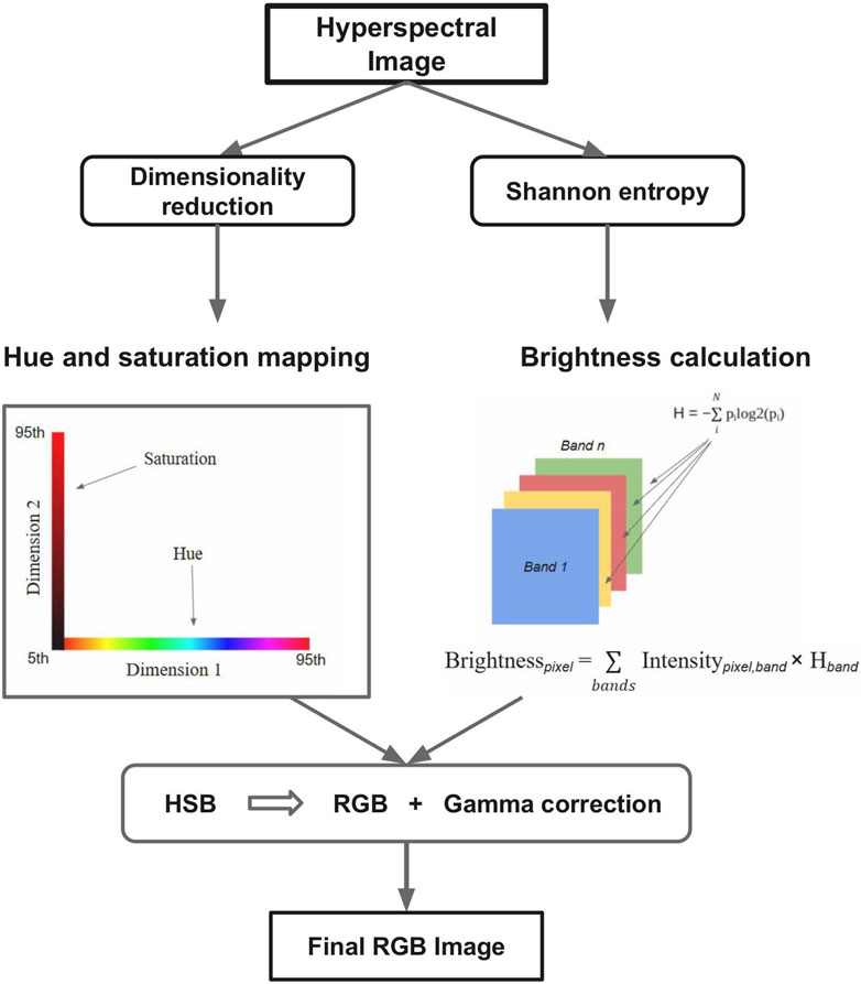
Figure 1. Flowchart of the key steps of the HSBDR-H approach.

2.1 Dimension reduction and color encoding

Prior to dimension reduction, each pixel’s spectral vector is first normalized per band to reduce the influence of absolute intensity differences:

${\stackrel{\sim }{x}}_{i,j}=x_{i,j}\text{/}\mathit{max}\left(x_j\right),$

where x _{i, j} is the intensity of pixel i in band j and max (x_j) is the maximum intensity of band j across all pixels.

A dimension reduction technique is then applied to map the high-dimensional spectral vectors into two dimensions:

$y_i=DR\left({\stackrel{\sim }{x}}_i\right)=\left[y_i^{\left(1\right)},y_i^{\left(2\right)}\right],$

The reduced dimensions are robustly normalized using the 5th and 95th percentiles to limit the effect of outliers:

$c_i^{\left(d\right)}=\frac{\mathit{min}(\mathit{max}\left(y_i^{\left(d\right)}-{P5}^{\left(d\right)},0\right),\left({P95}^{\left(d\right)}-{P5}^{\left(d\right)}\right)}{{P95}^{\left(d\right)}-{P5}^{\left(d\right)}},d=1,2,$

where P₅^(d) and P₉₅^(d) are the 5th and 95th percentiles of the dth reduced dimension, respectively. The first normalized dimension (c_i⁽¹⁾) is mapped to hue, and the second (c_i⁽²⁾) is mapped to saturation.

2.2 Entropy calculation for spectral bands

Shannon entropy is computed for each spectral band in the hyperspectral image cube to quantify its information content. These entropy values serve as weights in the subsequent brightness mapping process, emphasizing bands that contribute more discriminative spectral information.

2.3 Entropy-weighted brightness mapping

An entropy-weighted sum is calculated for each pixel by multiplying the pixel’s spectral intensity values by their corresponding band entropy scores. This sum reflects the contribution of informative bands to each pixel’s overall brightness. The resulting brightness values are then scaled and normalized using the 5th and 95th percentiles to ensure robustness against outliers and extreme values.

${\text{Brightness}}_{pixel}={\displaystyle \sum _{bands}}{\text{Intensity}}_{pixel,band}\times H_{band}.$

2.4 RGB conversion and image enhancement

The hue, saturation, and brightness (HSB) values obtained from the previous steps are converted to the standard RGB color space using HSV-to-RGB transformation. A gamma correction is then applied to the RGB image to enhance perceptual contrast and improve visual clarity.

Comparison with other visualization methods: To evaluate the effectiveness of our proposed approach, we conducted a comparative analysis using several commonly adopted, fast, and unsupervised dimension reduction methods. These included PCA (Datta et al., 2017; Ali et al., 2019), singular value decomposition (SVD) (Klema and Laub, 1980; Tripathi and Garg, 2021), independent component analysis (ICA) (Zhu et al., 2011; Hyvärinen, 2013), and random projection (RP) (Vempala, 2004; Sevilla et al., 2016). In comparison, we evaluated a more advanced unsupervised dimension reduction technique based on an autoencoder neural network (AE NN) (Jaiswal et al., 2023). In this approach, the network compresses the high-dimensional spectral data into a 3-dimensional latent vector, which is then directly mapped to the RGB channels for visualization.

The PCA, ICA, SVD, and RP methods were implemented using the corresponding modules from scikit-learn (Pedregosa et al., 2011). The AE NN model was trained using the PyTorch package (Paszke et al., 2019). Image and plot creation were carried out using Matplotlib (Hunter, 2007; Bisong, 2019).

Perceptual color difference analysis: To quantify perceptual differences between water and coastal regions in the selected magnified area, a grid overlay was applied using Matplotlib to divide the grayscale band with the highest entropy into indexed sections. Representative grid cells were randomly selected from water and coastal areas, and the same coordinates were used to extract the corresponding regions from all visualization outputs (PCA, SVD, RP, ICA, their HSB-based variants, and AE NN). Each extracted region was converted from RGB to CIELAB color space using scikit-image’s rgb2lab function. Mean L*a*b* values were then computed for each region, and the perceptual color difference (ΔE₀₀) (Luo et al., 2001) between water and coastal areas was calculated using deltaE_ciede2000 from scikit-image. The resulting ΔE₀₀ values were used to generate a comparative bar graph across all visualization methods.

Quantitative image quality metrics: To quantitatively assess the informativeness and sharpness of the final images produced by our method, Shannon entropy (Arun, 2013) and Laplacian energy (Zhang et al., 2013) values were calculated.

The Shannon entropy was calculated using the following formula:

$\mathrm{H}=-{\displaystyle \sum _{i=1}^N}{p}_i{\log }_2\left(p_i\right),$

where p_i represents the probability of occurrence of the ith intensity level in the image.

The Laplacian energy was calculated with the Laplacian function of the OpenCV Python package (Zelinsky, 2009). For simplicity, the Laplacian energy values presented in tables and figures are divided by 10⁷.

Edge Detection: To assess structural detail, we applied Canny edge detection to each generated RGB image (Canny, 1986). Prior to edge extraction, all images were converted to grayscale using the luminance-preserving transformation implemented in scikit-image. Edge maps were then computed using the Canny operator with a Gaussian smoothing parameter of σ = 1.0, which effectively balances noise suppression and edge localization. For each image, the resulting binary edge map was used to calculate edge density, defined as the ratio of detected edge pixels to the total number of image pixels. This provided a quantitative measure of structural richness and boundary clarity.

Implementation and availability: The implementation of the proposed HSBDR-H method, along with all tested dimension reduction techniques and comparison methods, is available as example Jupyter Notebook files on GitHub at https://github.com/Vahe-Atoyan/HSBDR-H.

Experimental platform and configuration: All experiments were performed on a Linux workstation with the following specifications: OS: Linux 6.8.0–85-generic, Kernel: #85–22.04.1-Ubuntu SMP. The system was equipped with a 4-core CPU running at 2.46 GHz, 3.65 GB of RAM, and no dedicated GPU. Python 3.9.21 was used with NumPy 1.23.5, scikit-learn 1.6.1, and Matplotlib 3.9.4. The gamma correction parameter was set to 1.2.

To ensure fast and reliable reproducibility, the Conda environment has been exported as HSBDR-H.yml. It can be downloaded from GitHub and used to create a local environment with the command: conda env create -f HSBDR-H.yml

3 Results and discussion

Our approach assigns HSB values to every pixel, enabling each pixel to potentially display any color and its attributes. Pixels with high reflectance in the most informative bands appear brighter, while those with lower reflectance in these bands appear darker, enhancing contrast between areas. This effect was particularly evident in the Washington Mall dataset, where the water bodies were displayed in black, contrasting sharply with the bright and detailed buildings (Figure 2). In comparison, traditional PCA-, SVD-, RP-, and ICA-generated images lacked contrast, making it difficult for the human eye to quickly distinguish objects and areas of interest. To further illustrate the perceptual differences within the image regions, an area containing both a water body and adjacent coastal zones was selected and magnified (Figure 3). The band with the highest entropy was visualized in grayscale to demonstrate the selected area. To quantify perceptual differences, grid cells were defined over the magnified region, and several cells were randomly sampled from the water (blue) and coastal (green) zones. Mean CIELAB color values were calculated for each region, and the CIEDE2000 (ΔE₀₀) metric was applied to quantify perceptual color difference. Higher ΔE₀₀ values correspond to greater color contrast between the water and coastal regions (Figure 3c). Across all visualization methods, HSBDR-H approaches exhibited higher ΔE₀₀ values than their RGB-based counterparts, with HSBSVD-H also slightly surpassing AE NN.

Figure 2

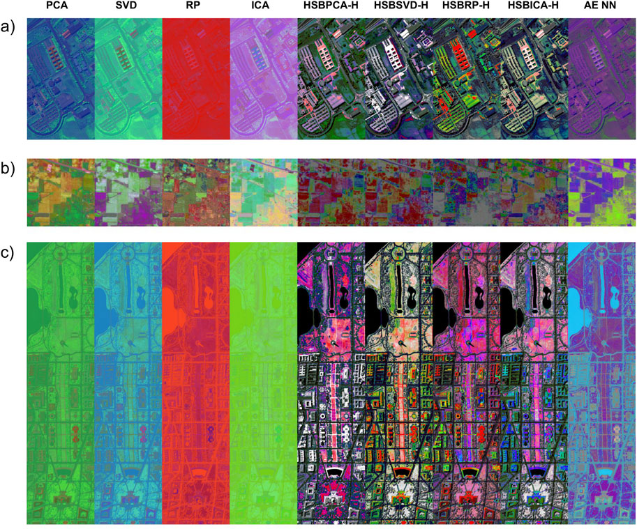
Figure 2. RGB visualizations of the (a) Pavia University, (b) Indian Pines, and (c) Washington Mall datasets using dimension reduction methods with traditional RGB mapping, shown alongside their corresponding HSBDR-H visualizations, and an autoencoder neural network (AE NN) approach.

Figure 3

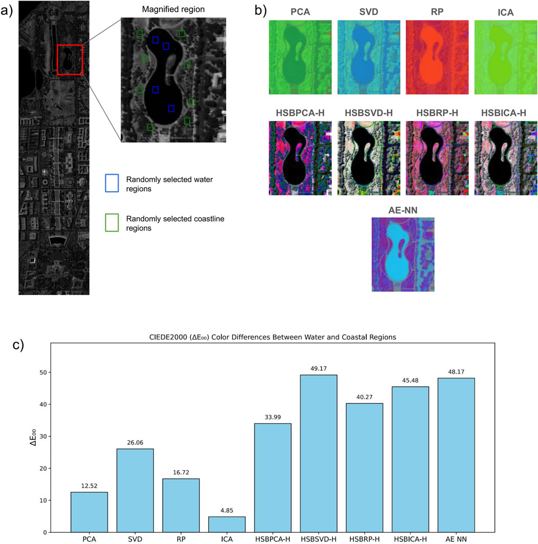
Figure 3. (a) Selected magnified region from the Washington Mall dataset, showing the randomly chosen water body (blue) and coastline (green) areas on the highest entropy band. (b) The same magnified region across all visualization techniques. (c) Bar graph of CIEDE2000 (ΔE₀₀) color differences between randomly selected water and coastal regions within the magnified area across all visualization techniques.

Variations in pixel hue, saturation, and brightness were also clearly demonstrated in the HSBDR-H plots (Figure 4). However, the Indian Pines dataset exhibited less pronounced differences in brightness, which was reflected in the resultant image, leading to a lower brightness contrast. This diminished performance is likely due to a shortage of high-entropy bands as many areas in the field display similar spectral characteristics. In contrast, AE NN demonstrated consistent image generation with balanced contrast across all tested datasets.

Figure 4

Figure 4. HSBDR-H plots of (a) Pavia University, (b) Indian Pines, and (c) Washington Mall datasets. The first reduced dimension represents the hue gradient, and the second corresponds to the saturation level. Both are normalized between the 5th and 95th percentiles to minimize the influence of outlier pixels on the color distribution. Brightness value is calculated using the discussed entropy-weighted approach.

Subjectively, the images produced by the HSBDR-H method exhibited greater overall informativeness, improved sharpness, and enhanced structural detail than traditional RGB visualizations, without a notable increase in computation time (Table 1). These qualitative observations were corroborated by quantitative analysis, as the HSBDR-H results demonstrated higher Shannon entropy, Laplacian energy, and edge density values, particularly for urban datasets (Tables 2–4).

Table 1

Table 1. Time (seconds) comparison of dimensionality reduction methods with traditional RGB mapping, shown alongside their corresponding HSBDR-H visualizations, and an autoencoder neural network (AE NN) approach.

Table 2

Table 2. Entropy comparison of dimensionality reduction methods with traditional RGB mapping, shown alongside their corresponding HSBDR-H visualizations, and an autoencoder neural network (AE NN) approach.

Table 3

Table 3. Laplacian energy comparison of dimensionality reduction methods with traditional RGB mapping, shown alongside their corresponding HSBDR-H visualizations, and an autoencoder neural network (AE NN) approach.

Table 4

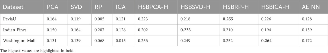
Table 4. Edge density comparison of dimensionality reduction methods with traditional RGB mapping, shown alongside their corresponding HSBDR-H visualizations, and an autoencoder neural network (AE NN) approach.

To evaluate the contribution and necessity of each key component in the proposed approach, an ablation study was conducted using HSBPCA-H on the Pavia University (PaviaU) dataset. First, the 5–95th percentile normalization was removed from all stages (hue, saturation, and brightness), and the resulting visualization was generated (1). Next, normalization was not applied to the brightness component but was applied to hue and saturation (2). Finally, to assess the importance of the proposed entropy-weighted brightness calculation, an additional version was generated using a constant brightness value for all pixels (3). Figure 5 presents these RGB visualizations, the complete HSBPCA-H pipeline, and the traditional PCA visualization along with their corresponding Canny edge maps. For all images, Shannon entropy, Laplacian energy, and edge density were computed and are displayed as bar charts, demonstrating that the full pipeline achieved the best overall performance among all tested configurations.

Figure 5

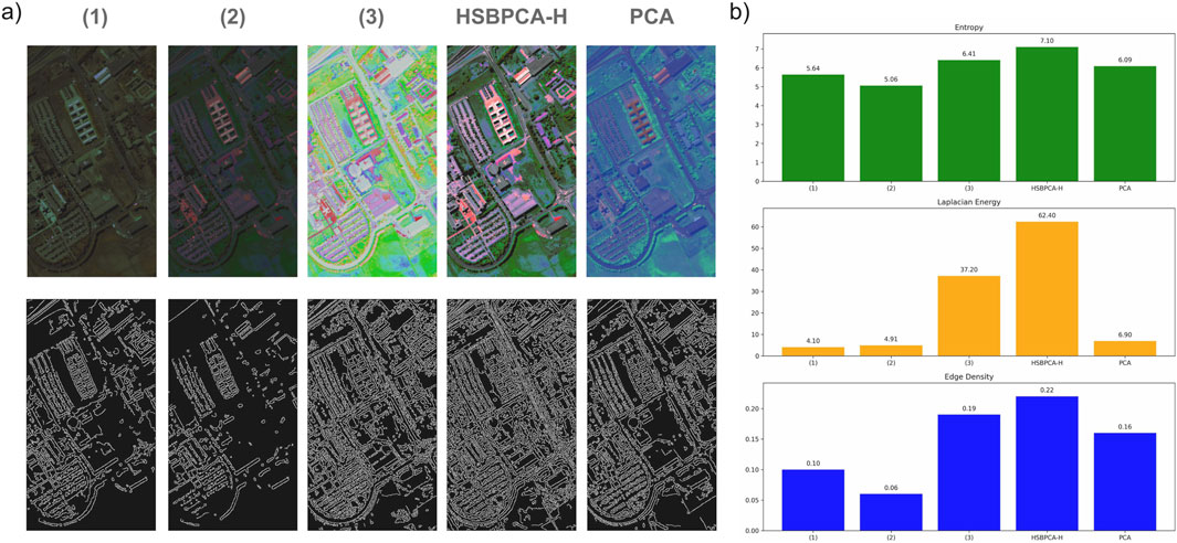
Figure 5. (a) Ablation study of the proposed HSBPCA-H visualization method on the Pavia University (PaviaU) dataset, showing RGB images (top) and corresponding Canny edge maps (bottom). (1) Without 5th–95th percentile normalization in any component (hue, saturation, and brightness); (2) with normalization applied only to hue and saturation but not brightness; and (3) with constant brightness assigned to all pixels. The figure also includes the complete HSBPCA-H pipeline and the traditional PCA visualization for comparison. (b) Bar plot of quantitative metrics—Shannon entropy, Laplacian energy, and edge density—demonstrating performance differences across configurations.

4 Conclusion

This study introduced HSBDR-H, a hyperspectral image visualization strategy that combines entropy-weighted brightness with hue and saturation derived from dimension reduction outputs. By moving beyond direct RGB mapping, the proposed approach provides more informative and contrast-rich representations of spectral data. It is compatible with a variety of dimension reduction techniques and incurs only a minimal increase in computation time. The method demonstrated enhanced visual contrast and structural detail in urban datasets, while achieving comparable performance to RGB-based approaches in field imagery.

To further improve computational efficiency—particularly for datasets with a large number of spectral bands—GPU-based parallelization of the Shannon entropy calculation could be employed as this computation is inherently non-sequential. In this study, such optimization was not implemented to ensure fair and hardware-independent timing comparisons.

Future research could explore alternative brightness calculation methods beyond Shannon entropy to improve performance on datasets with high spectral homogeneity (e.g., field datasets) as this represents a weakness of the current entropy-weighting approach. Additionally, given the growing number of dimension reduction techniques emerging across various fields (e.g., bioinformatics and bioimage analysis), it is worth investigating coupling these methods with the HSBDR-H approach as an interesting direction for expanding the method’s applicability and improving visualization quality across disciplines.

Data availability statement

The original contributions presented in the study are included in the article/supplementary material; further inquiries can be directed to the corresponding authors.

Author contributions

VA: Conceptualization, Methodology, Visualization, Writing – original draft, Writing – review and editing. TB: Methodology, Supervision, Writing – original draft, Writing – review and editing. LJ: Funding acquisition, Supervision, Writing – original draft, Writing – review and editing. AA: Funding acquisition, Supervision, Writing – original draft, Writing – review and editing.

Funding

The authors declare that financial support was received for the research and/or publication of this article. This work was funded via NordPlant Nordforsk [grant 84597] and the Higher Education and Science Committee of the Republic of Armenia [project 22IRF-10 “Climate change impact in Armenia: a holistic approach for studying the biodiversity of wild plant species”]. Vahe Atoyan’s visit to UiT was organized within the framework of the Erasmus+ program [project 2023-1-NO01-KA171-HED-000142440-UiT].

Conflict of interest

The authors declare that the research was conducted in the absence of any commercial or financial relationships that could be construed as a potential conflict of interest.

Generative AI statement

The authors declare that no Generative AI was used in the creation of this manuscript.

Any alternative text (alt text) provided alongside figures in this article has been generated by Frontiers with the support of artificial intelligence and reasonable efforts have been made to ensure accuracy, including review by the authors wherever possible. If you identify any issues, please contact us.

Publisher’s note

All claims expressed in this article are solely those of the authors and do not necessarily represent those of their affiliated organizations, or those of the publisher, the editors and the reviewers. Any product that may be evaluated in this article, or claim that may be made by its manufacturer, is not guaranteed or endorsed by the publisher.

References

Alam, A., Muqeem, M., and Ahmad, S. (2021). Comprehensive review on clustering techniques and its application on high dimensional data. IJCSNS Int. J. Comput. Sci. Netw. Secur. 21 (6), 237. doi:10.22937/IJCSNS.2021.21.6.31

CrossRef Full Text | Google Scholar

Ali, U. A. M. E., Hossain, Md. A., and Islam, M. R. (2019). Analysis of PCA based feature extraction methods for classification of hyperspectral image. Int. Conf. Innovation Eng. Technol. (ICIET), 1–6. doi:10.1109/iciet48527.2019.9290629

CrossRef Full Text | Google Scholar

Armstrong, G. E., Rahman, G., Martino, C., McDonald, D., Gonzalez, A., Mishne, G., et al. (2022). Applications and comparison of dimensionality reduction methods for microbiome data, Front. Bioinform. 2. 821861. doi:10.3389/fbinf.2022.821861

PubMed Abstract | CrossRef Full Text | Google Scholar

Arun, P. V. (2013). A comparative analysis on the applicability of entropy in remote sensing. J. Indian Soc. Remote Sens. 42 (1), 217–226. doi:10.1007/s12524-013-0304-1

CrossRef Full Text | Google Scholar

Balabathina, V. N., Mishra, S., Sharma, M., Sharma, S., Kumar, P., and Narayan, A. (2025). Comparative evaluation of fast-learning classification algorithms for urban forest tree species identification using EO-1 hyperion hyperspectral imagery. Front. Environ. Sci. 13, 1668746. doi:10.3389/fenvs.2025.1668746

CrossRef Full Text | Google Scholar

Baumgardner, M. F., Biehl, L. L., and Landgrebe, D. A. (2015). 220 band AVIRIS hyperspectral image Data Set: june 12, 1992 Indian Pine test site 3 [dataset] v1.0. West Lafayette, IN: Purdue University Research Repository. doi:10.4231/R7RX991C

CrossRef Full Text | Google Scholar

Bisong, E. (2019). “Matplotlib and seaborn,” in Building machine learning and deep learning models on google cloud platform, 151–165. doi:10.1007/978-1-4842-4470-8_12

CrossRef Full Text | Google Scholar

Calin, M. A., Parasca, S. V., Savastru, D., and Manea, D. (2013). Hyperspectral imaging in the medical field: present and future. Appl. Spectrosc. Rev. 49 (6), 435–447. doi:10.1080/05704928.2013.838678

CrossRef Full Text | Google Scholar

Canny, J. (1986). A computational approach to edge detection. IEEE Trans. Pattern Analysis Mach. Intell. PAMI-8 (6), 679–698. doi:10.1109/tpami.1986.4767851

PubMed Abstract | CrossRef Full Text | Google Scholar

Coliban, R.-M., Marincaş, M., Hatfaludi, C., and Ivanovici, M. (2020). Linear and non-linear models for remotely-sensed hyperspectral image visualization. Remote Sens. 12 (15), 2479. doi:10.3390/rs12152479

CrossRef Full Text | Google Scholar

Dale, L. M., Thewis, A., Boudry, C., Rotar, I., Dardenne, P., Baeten, V., et al. (2013). Hyperspectral imaging applications in agriculture and agro-food product quality and safety control: a review. Appl. Spectrosc. Rev. 48 (2), 142–159. doi:10.1080/05704928.2012.705800

CrossRef Full Text | Google Scholar

Datta, A., Ghosh, S., and Ghosh, A. (2017). PCA, kernel PCA and dimensionality reduction in hyperspectral images. Springer eBooks, 19–46. doi:10.1007/978-981-10-6704-4_2

CrossRef Full Text | Google Scholar

Dhande, A. P., Malik, R., Saini, D., Garg, R., Jha, S., Nazeer, J., et al. (2024). Design of a high-efficiency temporal engine for real-time spatial satellite image classification using augmented incremental transfer learning for crop analysis. SN Comput. Sci. 5, 585. doi:10.1007/s42979-024-02939-6

CrossRef Full Text | Google Scholar

Duan, P., Kang, X., Li, S., and Ghamisi, P. (2020). Multichannel pulse-coupled neural network-based hyperspectral image visualization. IEEE Trans. Geoscience Remote Sens. 58 (4), 2444–2456. doi:10.1109/tgrs.2019.2949427

CrossRef Full Text | Google Scholar

Fauvel, M., Benediktsson, J. A., Chanussot, J., and Sveinsson, J. R. (2008). Spectral and spatial classification of hyperspectral data using SVMs and morphological profiles. IEEE Trans. Geoscience Remote Sens. 46 (11), 3804–3814. doi:10.1109/tgrs.2008.922034

CrossRef Full Text | Google Scholar

Gewali, U. B., Monteiro, S. T., and Saber, E. (2018). Machine learning based hyperspectral image analysis: a survey. arXiv Cornell Univ. doi:10.48550/arxiv.1802.08701

CrossRef Full Text | Google Scholar

Goodenough, D. G., Chen, H., Gordon, P., Niemann, K. O., and Quinn, G. (2012). Forest applications with hyperspectral imaging. 7309–7312. doi:10.1109/igarss.2012.6351973

CrossRef Full Text | Google Scholar

Huang, X., Wu, L., and Ye, Y. (2019). A review on dimensionality reduction techniques. Int. J. Pattern Recognit. Artif. Intell. 33 (10), 1950017. doi:10.1142/s0218001419500174

CrossRef Full Text | Google Scholar

Hunter, J. D. (2007). Matplotlib: a 2D graphics environment. Comput. Sci. and Eng. 9 (3), 90–95. doi:10.1109/mcse.2007.55

CrossRef Full Text | Google Scholar

Hyvärinen, A. (2013). Independent component analysis: recent advances. Philosophical Trans. R. Soc. A Math. Phys. Eng. Sci. 371 (1984), 20110534. doi:10.1098/rsta.2011.0534

PubMed Abstract | CrossRef Full Text | Google Scholar

Jaiswal, G., Rani, R., Mangotra, H., and Sharma, A. (2023). Integration of hyperspectral imaging and autoencoders: benefits, applications, hyperparameter tunning and challenges. Comput. Sci. Rev. 50, 100584. doi:10.1016/j.cosrev.2023.100584

CrossRef Full Text | Google Scholar

Jhariya, A., Parekh, D., Lobo, J., Bongale, A., Jayaswal, R., Kadam, P., et al. (2024). Distance analysis and dimensionality reduction using PCA on brain tumour MRI scans. EAI Endorsed Transactions Pervasive Health Technology 10. doi:10.4108/eetpht.10.5632

CrossRef Full Text | Google Scholar

Karim, S., Qadir, A., Farooq, U., Shakir, M., and Laghari, A. A. (2023). Hyperspectral imaging: a review and trends towards medical imaging. Curr. Med. Imaging Former. Curr. Med. Imaging Rev. 19 (5), 417–427. doi:10.2174/1573405618666220519144358

PubMed Abstract | CrossRef Full Text | Google Scholar

Khan, M. J., Khan, H. S., Yousaf, A., Khurshid, K., and Abbas, A. (2018). Modern trends in hyperspectral image analysis: a review. IEEE Access 6, 14118–14129. doi:10.1109/access.2018.2812999

CrossRef Full Text | Google Scholar

Khonina, S. N., Kazanskiy, N. L., Oseledets, I. V., Nikonorov, A. V., and Butt, M. A. (2024). Synergy between artificial intelligence and hyperspectral imagining—A review. Technologies 12 (9), 163. doi:10.3390/technologies12090163

CrossRef Full Text | Google Scholar

Klema, V., and Laub, A. J. (1980). The singular value decomposition: its computation and some applications. IEEE Trans. Automatic Control 25 (2), 164–176. doi:10.1109/tac.1980.1102314

CrossRef Full Text | Google Scholar

Kurz, W., Wang, K., Bektas, F., Zhu, C., Kariper, E., Dong, X., et al. (2025). Dimensionality reduction in hyperspectral imaging using standard deviation-based band selection for efficient classification. Sci. Rep. 15, 34478. doi:10.1038/s41598-025-21738-4

PubMed Abstract | CrossRef Full Text | Google Scholar

Li, J., Bioucas-Dias, J. M., and Plaza, A. (2010). Semisupervised hyperspectral image segmentation using multinomial logistic regression with active learning. IEEE Trans. Geoscience Remote Sens. 48 (11), 4085–4098. doi:10.1109/tgrs.2010.2060550

CrossRef Full Text | Google Scholar

Li, P., Ebner, M., Noonan, P. J., Horgan, C. C., Bahl, A., Ourselin, S., et al. (2021). Deep learning approach for hyperspectral image demosaicking, spectral correction and high-resolution RGB reconstruction. Imaging and Visualization 10 (4), 409–417. doi:10.1080/21681163.2021.1997646

PubMed Abstract | CrossRef Full Text | Google Scholar

Li, Z., Chen, G., Li, G., Zhou, L., Pan, X., Zhao, W., et al. (2024). DBANet: dual-branch attention network for hyperspectral remote sensing image classification. Comput. Electr. Eng. 118, 109269. doi:10.1016/j.compeleceng.2024.109269

CrossRef Full Text | Google Scholar

Lu, B., Dao, P., Liu, J., He, Y., and Shang, J. (2020). Recent advances of hyperspectral imaging technology and applications in agriculture. Remote Sens. 12 (16), 2659. doi:10.3390/rs12162659

CrossRef Full Text | Google Scholar

Luo, M. R., Cui, G., and Rigg, B. (2001). The development of the CIE 2000 colour-difference formula: CIEDE2000. Color Res. and Appl. 26 (5), 340–350. doi:10.1002/col.1049

CrossRef Full Text | Google Scholar

Mehmood, M., Shahzad, A., Zafar, B., Shabbir, A., and Ali, N. (2022). Remote sensing image classification: a comprehensive review and applications. Math. Problems Eng. 2022, 1–24. doi:10.1155/2022/5880959

CrossRef Full Text | Google Scholar

Park, M.-S., Lee, J. K., Kim, B., Ju, H. Y., Yoo, K. H., Jung, C. W., et al. (2025). Assessing the clinical applicability of dimensionality reduction algorithms in flow cytometry for hematologic malignancies. Clin. Chem. Laboratory Med. (CCLM) 63 (7), 1432–1442. doi:10.1515/cclm-2025-0017

PubMed Abstract | CrossRef Full Text | Google Scholar

Paszke, A., Gross, S., Massa, F., Lerer, A., Bradbury, J., Chanan, G., et al. (2019). “PyTorch: an imperative style, high-performance deep learning library,” in Proceedings of the 33rd international conference on neural information processing systems (Red Hook, NY, USA: Curran Associates Inc.), 8026–8037.

Google Scholar

Pedregosa, F., Varoquaux, G., Gramfort, A., Michel, V., Thirion, B., Grisel, O., et al. (2011). Scikit-learn: machine learning in python. J. Mach. Learn. Res. 12, 2825–2830. doi:10.5555/1953048.2078195

CrossRef Full Text | Google Scholar

Pisani, M., and Zucco, M. (2018). Simple and cheap hyperspectral imaging for astronomy (and more). Proc. SPIE 10677, 5. doi:10.1117/12.2309835

CrossRef Full Text | Google Scholar

Purdue.edu (2025). MultiSpec© | home. Available online at: https://engineering.purdue.edu/biehl/MultiSpec/index.html (Accessed January 15, 2025).

Google Scholar

Ramakrishnan, D., and Bharti, R. (2015). Hyperspectral remote sensing and geological applications. Curr. Sci. 108 (5), 879–891. doi:10.2307/24216517

CrossRef Full Text | Google Scholar

Sanju, P. (2025). Advancing dimensionality reduction for enhanced visualization and clustering in single-cell transcriptomics. J. Anal. Sci. Technol. 16, 7. doi:10.1186/s40543-025-00480-6

CrossRef Full Text | Google Scholar

Sevilla, J., Martin, G., Nascimento, J., and Bioucas-Dias, J. (2016). “Hyperspectral image reconstruction from random projections on GPU,”IEEE Int. Geoscience Remote Sens. Symposium (IGARSS). 280–283. doi:10.1109/igarss.2016.7729064

CrossRef Full Text | Google Scholar

Sharma, A., Chopra, S. R., Sapate, S. G., Arora, K., Khalid, M., Jha, S., et al. (2024). Artificial intelligence techniques for landslides prediction using satellite imagery. IEEE Access 12, 117318–117334. doi:10.1109/access.2024.3446037

CrossRef Full Text | Google Scholar

Small, C., and Sousa, D. (2025). Multiscale topology of the spectroscopic mixing space: crystalline substrates. Front. Remote Sens. 6, 1551139. doi:10.3389/frsen.2025.1551139

CrossRef Full Text | Google Scholar

Sun, W., and Du, Q. (2019). Hyperspectral band selection: a review. IEEE Geoscience Remote Sens. Mag. 7 (2), 118–139. doi:10.1109/mgrs.2019.2911100

CrossRef Full Text | Google Scholar

Tripathi, P., and Garg, R. D. (2021). “Comparative analysis of singular value decomposition and eigen value decomposition based principal component analysis for Earth and lunar hyperspectral image,”11th Workshop Hyperspectral Imaging Signal Process. Evol. Remote Sens. (WHISPERS). 1–5. doi:10.1109/whispers52202.2021.9483978

CrossRef Full Text | Google Scholar

Vempala, S. S. (2004). “The random projection method,” in Theoretical computer science, 65. Providence, USA: American Mathematical Society. doi:10.1090/dimacs/065

CrossRef Full Text | Google Scholar

Wang, H., Ma, C., and Zhou, L. (2009). “A brief review of machine learning and its application,” in International conference on information engineering and computer science. Wuhan, China, 1–4. doi:10.1109/iciecs.2009.5362936

CrossRef Full Text | Google Scholar

Yoon, H., and Lee, J. (2022). “Hyperspectral image visualization through neural network for the food industry,”Evol. Remote Sens. (WHISPERS). 1–5. doi:10.1109/whispers56178.2022.9955049

CrossRef Full Text | Google Scholar

Zelinsky, A. (2009). Learning OpenCV-Computer Vision with the OpenCV Library (Bradski, G.R. et al.; 2008)[On the Shelf]. IEEE Robotics and Automation Mag. 16 (3), 100. doi:10.1109/mra.2009.933612

CrossRef Full Text | Google Scholar

Zhang, H., Bai, X., Zheng, H., Zhao, H., Zhou, J., Cheng, J., et al. (2013). Hierarchical remote sensing image analysis via graph laplacian energy. IEEE Geoscience Remote Sens. Lett. 10 (2), 396–400. doi:10.1109/lgrs.2012.2207087

CrossRef Full Text | Google Scholar

Zhang, W., Li, Z., Li, G., Zhuang, P., Hou, G., Zhang, Q., et al. (2023). GACNet: generate adversarial-driven cross-aware network for hyperspectral wheat variety identification. IEEE Trans. Geoscience Remote Sens. 62, 1–14. doi:10.1109/tgrs.2023.3347745

CrossRef Full Text | Google Scholar

Zhang, Y., Zhu, F., Liang, K., Lu, Z., Chen, Y., Zhong, X., et al. (2025). Estimating rice yield-related traits using machine learning models integrating hyperspectral and texture features. Front. Plant Sci. 16, 1713014. doi:10.3389/fpls.2025.1713014

PubMed Abstract | CrossRef Full Text | Google Scholar

Zhu, Y., Varshney, P. K., and Chen, H. (2011). ICA-based fusion for colour display of hyperspectral images. Int. J. Remote Sens. 32 (9), 2427–2450. doi:10.1080/01431161003698344

CrossRef Full Text | Google Scholar

Zhu, J., Wu, L., Hao, H., Song, X., and Lu, Y. (2017). “Auto-encoder based for high spectral dimensional data classification and visualization,”IEEE Second Int. Conf. Data Sci. Cybersp. (DSC). 350–354. doi:10.1109/dsc.2017.32

CrossRef Full Text | Google Scholar