 Ewa Matusiak
 Vasileios Chatziioannou
 Maarten Van Walstijn
- 1Department of Music Acoustics (IWK), University of Music and Performing Arts Vienna, Vienna, Austria
- 2Centre for Interdisciplinary Research in Music and Sound, School of Electronics, Electrical Engineering, and Computer Science, Queen’s University Belfast, Belfast, United Kingdom
In order to simulate the function of bowed string instruments, it is necessary to model the frictional interaction between the bow hair and the vibrating string. This is possible using an elasto-plastic friction model, which has previously succeeded in reproducing experimental data captured on a monochord setup. In this study, this elasto-plastic model is refined to guarantee passivity, and a stable numerical scheme is derived that inherits the energy balance of the underlying continuous model. The approach presented considers a finite-width bow, thus spreading the bow–string interaction over an area. The compliance of the bow hair and the torsional motion of the string are also taken into account. A sound example and animations of the string motion are provided to demonstrate the behavior of the model.
1 Introduction
In order to simulate bow–string interaction, it is crucial to accurately model the friction between string and bow. Several friction models—both static and dynamic—have been developed in recent decades. The static models were obtained after measuring the coefficient of friction either in a steady-state (see friction curve model suggested by Smith and Woodhouse (1999)) or in a transient part of the waveform (see friction curve model suggested by Galluzzo, 2004). Among existing dynamic friction models used to simulate string vibrations are an elasto-plastic friction model developed by Dupont et al. (2002) and first applied in bow–string simulations by Serafin et al. (2003) and a thermal model introduced by Woodhouse (2003) where the temperature of rosin is considered; it is implemented using digital waveguides in Maestre et al. (2014). Regardless of the modeling choice, it is essential to use a guaranteed-passive model along with a discretization method that preserves the energy-conservation properties of the continuous system (e.g., Chabassier and Joly, 2010; Bilbao et al., 2015; Desvages, 2018; Ducceschi and Bilbao, 2022; van Walstijn et al., 2024).
This study examines the application of the elasto-plastic friction model by Dupont et al. (2000) and Dupont et al. (2002) to numerical modeling of bow–string interaction. Their formulation is a refinement of the LuGre friction model (de Wit et al., 2024) which encountered drift at low sliding velocities. The idea behind the model is that two sliding surfaces are irregular at the microscopic level; their interaction is modelled as a bundle of elastic bristles, with each bristle contributing to the overall frictional force. This model has already been applied to bowed strings: it was implemented using a finite difference method in Willemsen et al. (2019), where it was applied to point-bowing a stiff string, and in Matusiak and Chatziioannou (2024), where it was applied to a finite-width bow model. A comparison between this elasto-plastic model and the thermal friction model introduced in Smith and Woodhouse (1999) was conducted in Serafin (2004) using both a digital waveguide implementation and a finite difference method locally under the bow. That study focused on highlighting the differences and similarities between these two dynamic friction models. It was demonstrated in Matusiak and Chatziioannou (2024) that, given the right set of parameters, the elasto-plastic friction model is able to reconstruct the steady-state as well as the transient of a measured waveform.
Although the elasto-plastic friction model has been successfully implemented in the above studies, the passivity of the model has not been thoroughly investigated. This is important in order to guarantee the stability of numerical simulations. In a recent study by Falaize and Roze (2024) on nonlinear interaction modelling, the Dupont model was incorporated in a Port-Hamiltonian formulation, which—besides the part related to the elastic bristles—can be shown to be passive. Passivity, however, is not guaranteed for the coupled bow–string interaction model, since the dissipation term associated with the bristle displacement can become negative for certain parameter values.
In this study, we re-examine this issue and propose a refined model which is shown to be passive for any model parameters. Such a refinement can also demonstrate the existence and uniqueness of solutions to the underlying differential equations. Furthermore, in order to numerically implement the model in a stable manner, an energy preserving discretization scheme is derived. This is an improvement on the implementation proposed in Willemsen (2021), where the numerical bristle energy was not guaranteed to be non-negative.
The paper is structured as follows. In Section 2, the elasto-plastic model is introduced in the context of a lumped bowed mass, and energy analysis is performed in the continuous domain to reveal the lack of passivity of the original elasto-plastic model. Section 3 presents a refined version of the model that preserves passivity and guarantees the uniqueness of the solution. Section 4 is concerned with the numerical formulation of the bowed mass model; discretization using the finite difference method and energy analysis in the discrete setting are performed, followed by numerical experiments and comparison of the two models. In Section 5, the friction model is applied to the problem of bowing a string with a bow of finite width. Transverse and torsional waves on the string are accounted for. Section 6 presents the numerical model for the bow–string interaction, including analysis of the discrete energy, and some concluding remarks are given in Section 7.
2 Elasto-plastic friction model
It is helpful to first present the problem in its simpler form, which involves modelling the bowing of a lumped mass connected to a stiff spring. This represents a specific case of the bowed string model, restricted solely to the transverse movement of a string that is bowed at a single contact point and considering only its fundamental mode of vibration (see Appendix).
Consider a bowed mass
where
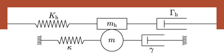
Figure 1. Sketch of the bowed lumped mass system.
Following Dupont et al. (2002), an elasto-plastic model is used to simulate the tangential friction force. This model assumes that the two surfaces—in this case the bow hair and the mass—are irregular at the microscopic level, and their contact is modelled through an ensemble of elastic bristles, each contributing to the total friction load. The bristles are modelled as damped stiff springs, and when the strain exceeds a certain breakaway threshold, the bristles break, and the two surfaces begin to slide. Denoting by
where
where
and where
and
with
2.1 Energy balance
In order to investigate the passivity of the model given by Equations 1–5, the energy balance of the system is considered.
Multiplying Equation 1 with
where
where
However, without knowing the maximal relative velocity,
Falaize and Roze (2024) employed the elasto-plastic friction model in the framework of port-Hamiltonian systems and arrived at the same dissipation term—
2.2 Boundedness of the bristle displacement
Boundedness of bristle displacement was first shown in Olsson (1996) for a LuGre friction model, and subsequently in Dupont et al. (2000) for an elasto-plastic model, by defining a positive definite Lyapunov function and an invariant set of solutions. Here a slightly different approach is presented.
The bristle displacement
and
This means that for
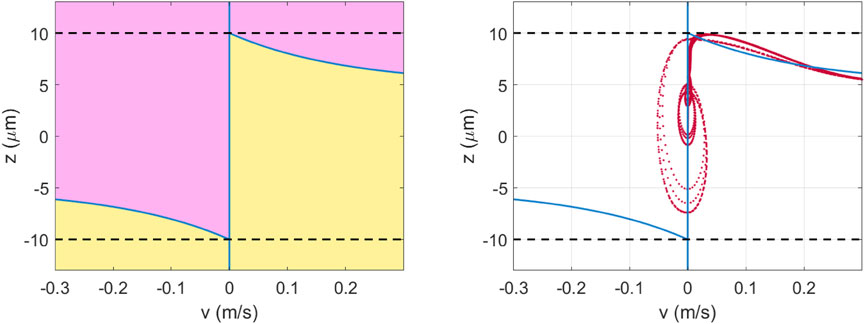
Figure 2. Behavior of the bristle displacement
3 Refined elasto-plastic model
This section presents a refined version of the elasto-plastic friction model that addresses the passivity of the system. Consider a mass
such that
A similar velocity-dependent damping term
3.1 Energy balance
With
Proposition 1: Let
Proof: All terms in the energy balance (Section 2.1) are trivially non-negative, apart from
3.2 Existence and uniqueness of the solution
The passivity of the system can be shown to guarantee the existence and uniqueness of the solution. By introducing a variable
Let
where
Definition 1:. A vector-valued function
If
The norm of
Proposition 2: Consider a bowed mass
Proof: By the Picard–Lindelöf theorem (Barreira and Valls, 2012), a system of ordinary differential equations
By passivity, all the variables are bounded. Lipschitz continuity of
is Lipschitz continuous.
(i) Let
where the last inequality follows from the Lipschitz continuity of the
Let
Hence,
(ii) Now, let
is continuous and everywhere differentiable except for
and
The partial derivative of
and
Let
Therefore,
The original Dupont model was not shown to be passive, as there was no guarantee that
4 Numerical formulation
In the present section, a finite difference numerical scheme is utilized to discretize the system in Equations 1–5. The proposed discretization is energy conserving.
4.1 Numerical preliminaries
The approximations to
In addition, one may define non-centered, first-order accurate discretization operators
The composition of first-order accurate operators results in second-order accurate operators,
and several useful identities can be constructed, including
4.2 Discretization
For simplicity of notation, let
The system of Equations 1–5 is discretized as follows:
In the case of the original Dupont model,
This discretization choice for the equation of motion of the lumped mass is motivated by the discretization that is carried out for the string model in the distributed case in Section 6. On the other hand, the stiffness term for the bow hair in Equation 26 is discretized using an averaging operator in order to avoid introducing a further stability condition.
For simpler notation, let
Substituting into Equations 25, 26, and 28, one obtains
Considering
where
For the original Dupont model,
An iterative solver, such as the Newton–Raphson method, can be applied to
in order to solve for
The solution of the nonlinear equation
4.3 Numerical energy balance
The stability of the numerical scheme is analyzed by investigating whether the discrete energy balance preserves the passivity of the underlying continuous system.
Multiplying Equation 25 with
Summing up the above and using relation Equation 27 yields
where
The energy balance in Equation 33 induces the following discrete conservation law (Chatziioannou and van Walstijn, 2015):
where
4.4 Numerical experiments
To demonstrate the behavior of the model, simulation results are shown in Figure 3. For these simulations, the bow accelerates from 0 at 3.439 m/s2 until it reaches the steady-state value
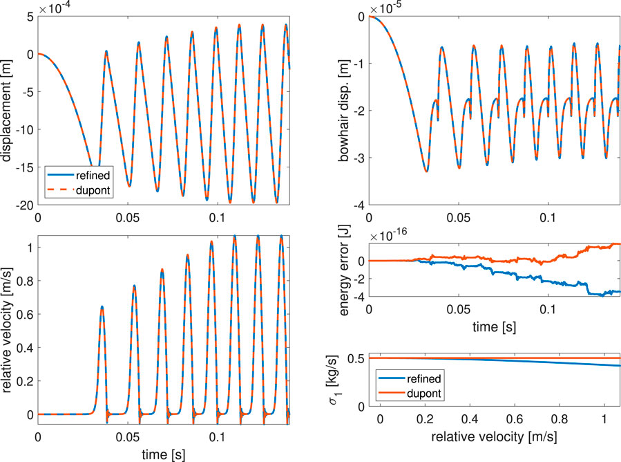
Figure 3. Comparison of the original (orange) and refined (blue) elasto-plastic friction model applied to simulating a bowed lumped mass. Model parameters are given in Table 1. Plotted signals are the mass displacement, bow hair displacement, relative velocity, and energy error, as defined in Equation 35. Bottom right plot shows the deviation of the bristle damping coefficient, in the case of the refined model, from the constant value
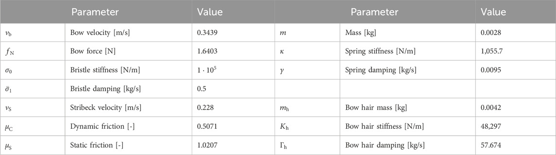
Table 1. Table with parameter values used to generate signals in Figure 3.
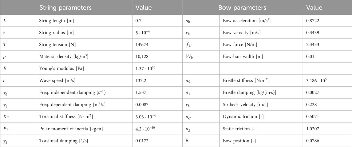
Table 2. Table with parameter values used to generate the signals in Figure 7. Bow-hair mass, stiffness, and damping are as in the lumped case (see Table 1), divided by the width of the bow hair.
For this parameter set, the refined model generates signals that are nearly identical to those generated by the original Dupont model. The latter has been used to simulate a string bowed by a finite-width bow and was validated against experimental measurements for the case of a monochord played by a bow (Matusiak and Chatziioannou, 2024). Therefore, it is possible to deduce that the refined model can also reliably resynthesize measured signals.
The difference between the two models comes into play when the Dupont model violates the passivity condition (Equation 34); the two models then behave quite differently (Figure 4). To generate this figure, the bristle stiffness
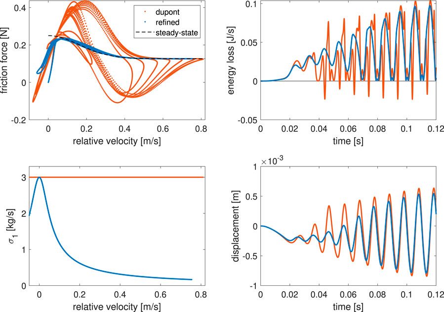
Figure 4. Comparison of the behavior of the original (orange) and refined (blue) elasto-plastic friction models when the passivity condition of the original model is violated. The total energy loss of the original model becomes negative, violating passivity, and the friction force deviates significantly from the underlying theoretical steady-state friction curve.
As discussed in Section 4.2, a further issue with this modeling approach is whether the system possesses a unique solution. This can only be shown for the refined model in the continuous case. For the discrete case, the uniqueness of the solution could only be demonstrated empirically. The nonlinear function
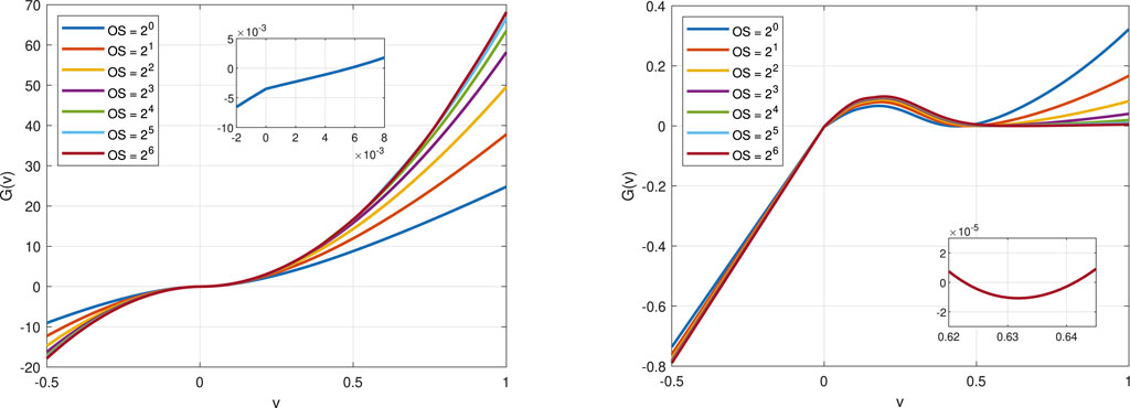
Figure 5. Nonlinear function
Furthermore, it is possible to observe that for both models, the derivative of
Finally, the convergence of the refined model is illustrated in Figure 6. A global error is defined, assuming a reference signal
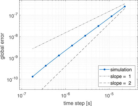
Figure 6. Error of the refined model for different time steps, as defined in Equation 36. Dashed line indicates second-order convergence, while dash-dotted line indicates first order convergence. Model parameters are taken from Table 1.
5 Distributed system
The insights obtained while studying the bowed-mass system are now applied to a distributed system—a string bowed with a finite width bow. In the following, let
Using the subscripts
where
5.1 String model
The governing equations for the motion of a string excited by a bow are the equations describing transverse (Equation 39) and torsional (Equation 40) waves. They are coupled through the distributed friction force
where
This model simplifies string damping and omits body coupling. This simplified approach is favored in this case, as including these additional factors would not enhance the presentation of the friction model.
Assuming simply supported ends, the boundary conditions for the transverse movement of the string are
and for the torsional movement we assume fixed boundary conditions
A fourth equation, needed to close the system, describing the friction force
where
where the adhesion map
5.2 Energy analysis
The time derivative of the total energy of the combined transverse and torsional movement of the string, bow hair, and bristle energy may be derived by taking an inner product of Equations 39, 40, 41, and 46 with
where
and
The dissipated energies in the string (
and the boundary terms are
Under simply supported boundary conditions,
Given that
since, by Proposition 1, the expression under the integral is positive if
6 Distributed system—Numerical formulation
6.1 Operators and identities
Let
Other domains that differ from
The time difference and averaging operators introduced in Sections 4.1, 4.2 are valid in their implementation to grid functions. Similarly, as in the continuous case, the following identities hold:
Spatial forward, backward, and central discretization operators are defined as
and can be used to obtain approximations to higher-order partial differential operators:
Like in the continuous case, the following relation can be derived:
6.2 Discretization
Finite-difference schemes for the string in isolation and the bowed string have been described in studies such as Bilbao (2009) and Pitteroff and Woodhouse (1998b). In order to fix the notation, let
The model is discretized in time and space with functions
where
where
For a point
To simplify the notation, we first divide Equation 39 by
where
with
for
then
Assuming simply supported ends, the boundary conditions imply
for all
Similarly, by dividing Equation 40 by
where
for all
Discretization of the equation governing bow hair displacement is performed as in the lumped case:
where
where
where
where
In order to update the system variables, the vectors
The system can then be solved for
where
where
with
Note that Equations 60 and 61 can be reduced to solving just one equation, as was performed in the case of the bowed lumped mass. Using Equation 60 and writing the friction force in terms of
the bristle displacement can be expressed as
where
6.3 Numerical energy and stability condition
An energy balance for the discretized scheme follows from a discrete inner product of Equation 52 with
where
The total energy lost due to damping is defined as
where
For simply supported and fixed boundary conditions, the boundary term
The bowed string model is passive, and the argument follows that in the continuous case, where the integral becomes the sum:
Non-negativity of
6.4 Numerical experiments
Simulated signals using the refined bow–string interaction model are shown in Figure 7. In this case, the bow starts in contact with the string, and the force is kept constant while the bow is accelerated from rest with a chosen acceleration value until the steady-state bow velocity
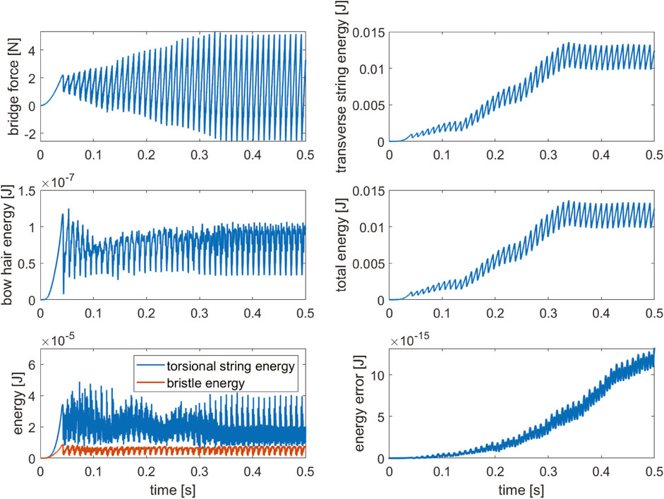
Figure 7. Simulated bridge force using the refined elasto-plastic model, along with various energy components. Total energy is the sum of the transverse and torsional energies of the string as well as the bristle and bow hair energies. The energy error is shown on the bottom right. Model parameter values are given in Table 2.
The original Dupont friction model was recently applied to the distributed case of bowing a string in Matusiak and Chatziioannou (2024). The performance of the original elasto-plastic model was evaluated by simulating a Guettler diagram and comparing it to a Guettler diagram obtained from measurements (Lampis et al., 2024). A Guettler diagram is generated by choosing a fixed location on the string and bowing from rest with an accelerating bow. The bow force while bowing is kept constant. Bowing is then repeated for different accelerations and bow forces that are incremented in small steps. The number of periods required to reach Helmholtz motion is visualized via the color of each pixel (Figure 8). White corresponds to 0 periods (perfect transient) and black to 20 periods, with intermediate transient lengths resulting in different grayscale values. Guettler (2002) proposed such a diagram as a measure of assessing the playability of a bowed string by measuring the length of the transient necessary to arrive at Helmholz motion.
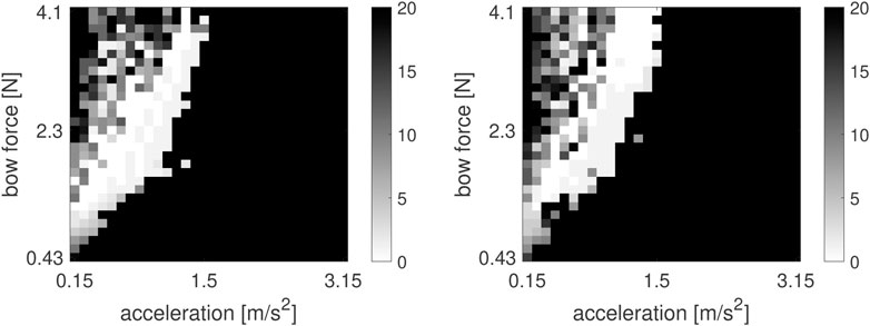
Figure 8. Guettler diagrams using Dupont (left) and refined models (right) with string parameters as in Table 2. The color bar refers to the number of periods required for Helmholtz motion to be achieved (transient length).
The refined model was utilized to simulate a Guettler diagram with the same parameters as in Matusiak and Chatziioannou (2024). The two diagrams are shown in Figure 8 for comparison. The chaotic nature of the frictional interaction manifests itself via the patchiness of the playability regions. Neighboring pixels may correspond to largely different transient durations, indicating sensitivity to small changes in bow force and acceleration. Therefore, the diagrams slightly differ due to the small underlying numerical differences of the two models. Qualitative observations regarding the playability of the system are nevertheless the same for both models.
6.5 Supplementary material
A sound example of the synthesis of a fast sautillé passage is included in the supplementary material. Simulation of this bow stroke style exposes the transient behavior of the proposed bow–string model and offers the reader a preliminary aural impression of it. For synthesis of the G2 notes, the bow velocity and force were varied periodically over time according to patterns similar to those observed in Demoucron (2008). Convolution with a measured cello impulse response was applied to the bridge force signal to render a more realistic audio signal.
Furthermore, animations of the string motion are provided for the case shown in Figure 7, where Helmholtz motion is achieved, as well as for a case where the bow force is reduced by 50% (
7 Conclusion
An elasto-plastic friction model has been investigated from the point of view of energy conservation in the continuous domain and discretized using a finite difference scheme. The model was first analyzed in the setting of a bowed lumped mass. A refinement of the model has been suggested that guarantees passivity for elasto-plastic friction with the Stribeck effect and simultaneously leads to the existence and uniqueness of the solution. A numerical scheme has been derived that respects the energy balance of the underlying continuous model, thus leading to a guaranteed passive model and hence to stable simulations.
Based on this refined version of the elasto-plastic model, simulations of a bowed string were revisited, including bow compliance, string torsion, and a finite bow width. While results are similar to those previously obtained using the original Dupont model, the refined model presented is proven to be guaranteed passive, as is the case for the lumped system.
The main limitation of the proposed implicit scheme is that the Jacobian of the nonlinear function to be solved iteratively at each time step can become singular, which—even when applying deliberately modified versions of the iterative solver (e.g., Hueso et al. 2009)—can lead to the necessity of a huge number of iterations. In practice, this often necessitates heavy oversampling, especially when driving the model with articulation parameters (e.g., bowing force) that vary across over time. A logical future research direction is therefore to develop numerical schemes that sidestep the need for an iterative solver, as has been achieved recently for numerical simulation of various other nonlinear phenomena in musical instruments, including collisions (e.g., van Walstijn et al., 2024).
Data availability statement
The original contributions presented in the study are included in the article/Supplementary Material; further inquiries can be directed to the corresponding author.
Author contributions
EM: conceptualization, investigation, methodology, software, and writing – original draft. VC: funding acquisition, investigation, project administration, validation, and writing – review and editing. MV: investigation, validation, and writing – review and editing.
Funding
The author(s) declare that financial support was received for the research and/or publication of this article. This research was funded in whole or in part by the Austrian Science Fund (FWF) [10.55776/P34852]. For open access purposes, the authors have applied a CC BY public copyright license to any author-accepted manuscript version arising from this submission.
Conflict of interest
The authors declare that the research was conducted in the absence of any commercial or financial relationships that could be construed as a potential conflict of interest.
Generative AI statement
The author(s) declare that no Generative AI was used in the creation of this manuscript.
Publisher’s note
All claims expressed in this article are solely those of the authors and do not necessarily represent those of their affiliated organizations, or those of the publisher, the editors and the reviewers. Any product that may be evaluated in this article, or claim that may be made by its manufacturer, is not guaranteed or endorsed by the publisher.
Supplementary material
The Supplementary Material for this article can be found online at: https://www.frontiersin.org/articles/10.3389/frsip.2025.1525044/full#supplementary-material
References
Barreira, L., and Valls, C. (2012). Ordinary differential equations: qualitative theory. America, American Mathematical Society.
Bilbao, S., Torin, A., and Chatziioannou, V. (2015). Numerical modeling of collisions in musical instruments. Acta Acust. United Acust. 101, 155–173. doi:10.3813/AAA.918813
Chabassier, J., and Joly, P. (2010). Energy preserving schemes for nonlinear Hamiltonian systems of wave equations: application to the vibrating piano string. Comput. Methods Appl. Mech. Eng. 199, 2779–2795. doi:10.1016/j.cma.2010.04.013
Chatziioannou, V., and van Walstijn, M. (2015). “Discrete-time conserved quantities for damped oscillators,” in Proceedings of the third Vienna talk on music acoustics (Vienna, AT: Department of Music Acoustics - Wiener Klangstil), 135–139.
Demoucron, M. (2008). On the control of virtual violins physical modelling and control of bowed string instruments (Stockholm: Royal Institute of Technology). Ph.D. thesis.
Desvages, C. (2018). Physical modelling of the bowed string and applications to sound synthesis (The University of Edinburgh). Ph.D. thesis.
Deuflhard, P. (2011). Newton methods for nonlinear problems: affine invariance and adaptive algorithms. Springer Sci. and Bus. Media 35.
de Wit, C., Olsson, H., Åström, K., and Lischinsky, P. (2024). A new model for control of systems with friction. IEEE Trans. Autom. Control 40, 419–425. doi:10.1109/9.376053
Ducceschi, M., and Bilbao, S. (2022). Simulation of the geometrically exact nonlinear string via energy quadratisation. J. Sound Vib. 534, 117021. doi:10.1016/j.jsv.2022.117021
Dupont, P., Armstrong, B., and Hayward, V. (2000). Elasto-plastic friction model: contact compliance and stiction. Proc. 2000 Acc. IEEE Chic., 1072–1077 vol.2. doi:10.1109/ACC.2000.876665
Dupont, P., Hayward, V., Armstrong, B., and Altpeter, F. (2002). Single state elasto-plastic friction models. IEEE Trans. Autom. Control 47, 787–792. doi:10.1109/TAC.2002.1000274
Falaize, A., and Roze, D. (2024). Generic passive-guaranteed nonlinear interaction model and structure-preserving spatial discretization procedure with applications in musical acoustics. Nonlinear Dyn. 112, 3249–3275. doi:10.1007/s11071-024-10438-9
Galluzzo, P. (2004). On the playability of stringed instruments. Ph.D. thesis. doi:10.17863/CAM.14046
Guettler, K. (2002). On the creation of the helmholtz motion in bowed strings. Acta Acust. united Acust. 88, 970–985.
Hueso, J., Martínez, E., and Torregrosa, J. (2009). Modified Newton’s method for systems of nonlinear equations with singular Jacobian. J. Comput. Appl. Math. 224, 77–83. doi:10.1016/j.cam.2008.04.013
Lampis, A., Mayer, A., and Chatziioannou, V. (2024). Assessing playability limits of bowed-string transients using experimental measurements. Acta Acust. 8, 44. doi:10.1051/aacus/2024034
Maestre, E., Spa, C., and Smith, J. (2014). A bowed string physical model including finite-width thermal friction and hair dynamics. ICMC.
Matusiak, E., and Chatziioannou, V. (2024). Elasto-plastic friction modeling toward reconstructing measured bowed-string transients. J. Acoust. Soc. Am. 156, 1135–1147. doi:10.1121/10.0028228
Pitteroff, R., and Woodhouse, J. (1998a). Mechanics of the contact area between a violin bow and a string. Part I: reflection and transmission behaviour. Acta Acust. United Acust. 84, 543–562.
Pitteroff, R., and Woodhouse, J. (1998b). Mechanics of the contact area between a violin bow and a string. Part II: simulating the bowed string. Acta Acust. United Acust. 84, 744–757.
Serafin, S. (2004). The sound of friction: real-time models, playability and musical applications (Stanford: Stanford University). Ph.D. thesis.
Serafin, S., Avanzini, F., and Rocchesso, D. (2003). “Bowed string simulations using an elasto-plastic friction model,” in Proceedings of the Stockholm Music Accoustics Conference, USA, 14–15 June 2023.
Smith, J., and Woodhouse, J. (1999). The tribology of rosin. J. Mech. Phys. Solids 48, 1633–1681. doi:10.1016/S0022-5096(99)00067-8
van Walstijn, M., Chatziioannou, V., and Bhanuprakash, A. (2024). Implicit and explicit schemes for energy-stable simulation of string vibrations with collisions: refinement, analysis, and comparison. J. Sound Vib. 569, 117968. doi:10.1016/j.jsv.2023.117968
Willemsen, S. (2021). “Real-time simulation of musical instruments using finite-difference time-domain methods,”.Aalb. Univ. Ph.D. thesis. doi:10.54337/aau451025772
Willemsen, S., Bilbao, S., and Serafin, S. (2019). Real-time implementation of an elasto-plastic friction model applied to stiff strings using finite-difference schemes. Proceedings of the International Conference on Digital Audio Effects, USA, 8-10 Sept. 2021, 40–46.
Woodhouse, J. (2003). Bowed string simulation using a thermal friction model. Acta Acustica united Acustica 89, 355–368. doi:10.25144/18216
Appendix
The modal expansion for the displacement of the string, assuming simply supported boundary conditions, is
where
and an inner product with
where
Therefore, by setting
Keywords: bowed mass, bow–string interaction, friction, passivity, finite differences, energy methods, numerical stability, elasto-plastic
Citation: Matusiak E, Chatziioannou V and Van Walstijn M (2025) Numerical modelling of elasto-plastic friction in bow–string interaction with guaranteed passivity. Front. Signal Process. 5:1525044. doi: 10.3389/frsip.2025.1525044
Received: 08 November 2024; Accepted: 11 March 2025;
Published: 21 May 2025.
Edited by:
Augusto Sarti, Polytechnic University of Milan, ItalyReviewed by:
Sorin Vlase, Transilvania University of Brașov, RomaniaSilviu Nastac, Dunarea de Jos University, Romania
Copyright © 2025 Matusiak, Chatziioannou and Van Walstijn. This is an open-access article distributed under the terms of the Creative Commons Attribution License (CC BY). The use, distribution or reproduction in other forums is permitted, provided the original author(s) and the copyright owner(s) are credited and that the original publication in this journal is cited, in accordance with accepted academic practice. No use, distribution or reproduction is permitted which does not comply with these terms.
*Correspondence: Ewa Matusiak, bWF0dXNpYWtAbWR3LmFjLmF0