Structural properties and asymptotic behavior of bacterial two-component systems

Bacteria rely on two-component signaling systems (TCSs) to detect environmental cues and orchestrate adaptive responses. Despite their apparent simplicity, TCSs exhibit a rich spectrum of dynamic behaviors arising from network architectures, such as bifunctional enzymes, multi-step phosphorelays, transcriptional feedback loops, and auxiliary interactions. This study develops a generalized mathematical model of a TCS that integrates these various elements. Using systems-level analysis, we elucidate how network architecture and biochemical parameters shape key properties such as stability, monotonicity, and signal amplification. Analytical conditions are derived for when the steady-state levels of phosphorylated proteins exhibit robustness to variations in protein abundance. The model characterizes how equilibrium phosphorylation levels depend on the absolute and relative abundances of the two components. Specific scenarios are explored, including the MprAB system from Mycobacterium tuberculosis and the EnvZ/OmpR system from textit Escherichia coli, to describe the potential role of reverse phosphotransfer reactions. By combining mechanistic modeling with system-level techniques, such as nullcline analysis, this study offers a unified perspective on the design principles underlying the versatility of bacterial signal transduction. The generalized modeling framework lays a theoretical foundation for interpreting experimental dynamics and rationally engineering synthetic TCS circuits with prescribed response dynamics.

1 Introduction

Bacteria rely on two-component systems (TCSs) as their primary signaling modules to detect environmental cues and orchestrate adaptive responses. A canonical TCS consists of a membrane-bound sensor histidine kinase (SHK) and a cytoplasmic response regulator (RR). Upon stimulation, the SHK autophosphorylates on a conserved histidine and transfers the phosphoryl group to an aspartate on the RR, generating the active form (RR-P) that typically regulates gene expression. This minimal architecture is remarkably versatile, underpinning processes such as chemotaxis, nutrient sensing, antibiotic resistance, and virulence regulation (Tierney and Rather, 2019; Tiwari et al., 2017; Kirby, 2009; Ramos et al., 2022; Alvarez and Georgellis, 2023).

Despite their apparent simplicity, TCSs display a rich spectrum of topologies and dynamic behaviors (Zschiedrich et al., 2016; Groisman, 2016; Stock et al., 2000). In some systems, exemplified by CheA in bacterial chemotaxis, SHK functions exclusively as a kinase, phosphorylating the RR. However, in many TCSs, SHK is bifunctional, participating in both phosphorylation and dephosphorylation of its cognate RR. In such cases, the input signal can modulate either one or both of these enzymatic activities, effectively tuning the rates of kinase and/or phosphatase reactions. TCSs may implement single-step phosphotransfers or multi-step phosphorelays, adding regulatory complexity and potentially delaying signal propagation.

At the transcriptional level, many TCSs feature autoregulation: the phosphorylated RR activates transcription of both its own gene and the gene encoding its partner SHK, thereby forming a positive feedback loop (Goulian, 2010). This feedback can alter steady-state behavior, activation, and inactivation kinetics and generate transient overshoot or “memory” effects, whereby the system responds faster to repeated stimuli. Although less common, negative autoregulation—or even mixed positive and negative feedback—has been observed in specific systems, providing an additional layer of response modulation. Auxiliary proteins can further diversify TCS behaviors, either by directly interacting with SHKs or RRs or by mediating cross-talk between otherwise independent TCS pathways (Rao et al., 2021; Groisman, 2016).

Mathematical modeling has been pivotal in elucidating the emergent properties of TCSs (summarized in Table 1). Batchelor and Goulian (2003) demonstrated that the steady-state level of RR-P can be robust to protein abundance fluctuations when SHK is limiting, a property supported by experimental data. Shinar et al. (2007) formalized the conditions for input-output robustness, showing that robustness is compromised when multiple independent phosphorylation or dephosphorylation routes exist. Igoshin et al. (2008) identified conditions for bistability, particularly when unphosphorylated SHK and RR form “dead-end” complexes or when alternative phosphatases modulate RR-P turnover. Ray and Igoshin (2010), Mitrophanov et al. (2010), and Zorzan et al. (2021) explored the role of transcriptional feedback, showing that autoregulation can alter response speed, overshoot amplitude, and even affect the effective sign of feedback, enabling TCSs to switch between positive and negative regulatory modes depending on signal strength. These studies collectively highlight how bifunctionality, phosphorelays, and feedback loops produce rich dynamic behaviors—including robustness, bistability, and adaptive memory—that are now central themes in systems-level analyses of TCSs.

Table 1

Table 1. Comparison of previous findings on bacterial TCSs with results from this study’s model.

In this study, we develop a systems-level model of a generalized TCS model focusing on the MprAB system from Mycobacterium tuberculosis that integrates canonical phosphorylation cycles, bifunctional enzymatic activity, transcriptional feedback, and potential auxiliary interactions. Our modeling framework seeks to (i) dissect how network architecture and parameter regimes shape dynamic properties and provide robustness, to be adopted as a building block to implement overshoots, oscillations, and bistability, and (ii) provide a predictive foundation for interpreting experimental dynamics and guiding synthetic circuit design in bacterial signal transduction.

By combining mechanistic modeling with systems-level analysis, this study elucidates how bifunctionality, phosphorelays, and feedback loops shape the dynamic behavior of TCSs, providing insights into bacterial adaptation and a framework for the rational engineering of synthetic signaling circuits (Mukherji and van Oudenaarden, 2009; Pasotti et al., 2017; Müller et al., 2025).

2 Two-component system: mathematical model

The model we consider is a general version of the model proposed in Tiwari et al. (2010) to describe the functioning of the two-component system MprA/MprB in M. tuberculosis in its active state.

For the sake of generality, we refer to “response regulator” $(RR)$ and “sensor histidine kinase” $(SHK)$ rather than to MprA and MprB, respectively. Denoting by $r$ $(r^{*})$ and $s$ $(s^{*})$, the concentration of $RR$ (phosphorylated $RR$) and $SHK$ (phosphorylated $SHK$), respectively, the dynamic evolution of the two-component system is described by the following set of ODEs (see Supplemental Information of Tiwari et al. (2010), Equations (S39)–(S42)):

$\dot{r}=\frac{k_p}{K_P}{r}^{*}s-\frac{k_t}{K_T}r{s}^{*}+k_{\mathit{exd}}{r}^{*}-k_{\mathit{exp}}r+{\nu }_r-k_{\mathit{pdeg}}r(1)$

${\dot{r}}^{*}=-\frac{k_p}{K_P}{r}^{*}s+\frac{k_t}{K_T}r{s}^{*}-k_{\mathit{exd}}{r}^{*}+k_{\mathit{exp}}r-k_{\mathit{pdeg}}{r}^{*}(2)$

$\dot{s}=k_{ad}{s}^{*}-k_{ap}s+\frac{k_t}{K_T}r{s}^{*}+{\nu }_s-k_{\mathit{pdeg}}s(3)$

${\dot{s}}^{*}=-k_{ad}{s}^{*}+k_{ap}s-\frac{k_t}{K_T}r{s}^{*}-k_{\mathit{pdeg}}{s}^{*}(4)$

—where

$•$ ${\nu }_r$ and ${\nu }_s$ are the production rate constants of $RR$ and $SHK$, respectively;¹

$•$ $k_p$ is the rate constant for the $SHK$-dependent dephosphorylation of $R{R}^{*}$;

$•$ $K_P$ is the Michaelis–Menten constant for $R{R}^{*}$ dephosphorylation by $SHK$;

$•$ $k_t$ is the rate constant for the $SH{K}^{*}$-dependent phosphorylation of $RR$;

$•$ $K_T$ is the Michaelis–Menten constant for $RR$–$SH{K}^{*}$ phosphotransfer;

$•$ $k_{\mathit{exp}}$ and $k_{\mathit{exd}}$ are the exogenous phosphorylation and dephosphorylation rate constants, respectively;

$•$ $k_{ap}$ and $k_{ad}$ are the autophopshorylation and autodephosphorylation rate constants, respectively;

$•$ $k_{\mathit{pdeg}}$ is the protein degradation rate (assumed equal for $RR$ and $SHK$).

One additional assumption worth highlighting is that the system is always considered to be in the active state. This is biologically reasonable as external stimuli often saturate the sensing capacity of the TCS. As a result, the transition of the sensor $s$ from the inactive to the active state upon binding external stimuli can be neglected in the model, as well as the availability of ATP inside the cell to provide phosphate groups for the phosphorylation steps.

The overall system can be represented as in Figure 1.

Figure 1

Figure 1. Schema of the generalized TCS. Binding of the signal molecule and general activation of genes are reported in panel (a), while in panel (b) the part of the system described by Equations 1–4 is reported.

We define the total amount of $RR$ and $SHK$ as $R_T=r+r^{*}$ and $S_T=s+s^{*}$, respectively, and rewrite the previous model presented in Equations 1–4 in the form shown in Equations 5–8:

${\dot{R}}_T=k_{\mathit{pdeg}}\left(u_r-R_T\right)(5)$

${\dot{r}}^{*}=-\frac{k_p}{K_P}{r}^{*}\left(S_T-s^{*}\right)+\frac{k_t}{K_T}\left(R_T-r^{*}\right)s^{*}-k_{\mathit{exd}}{r}^{*}+k_{\mathit{exp}}\left(R_T-r^{*}\right)-k_{\mathit{pdeg}}{r}^{*}(6)$

${\dot{S}}_T=k_{\mathit{pdeg}}\left(u_s-S_T\right)(7)$

${\dot{s}}^{*}=-k_{ad}{s}^{*}+k_{ap}\left(S_T-s^{*}\right)-\frac{k_t}{K_T}\left(R_T-r^{*}\right)s^{*}-k_{\mathit{pdeg}}{s}^{*}(8)$

—where $u_r≔{\nu }_r/k_{\mathit{pdeg}}$ $(u_s≔{\nu }_s/k_{\mathit{pdeg}})$ is the net production rate of $RR$ $(SHK)$. Due to the separation of timescales between protein accumulation and phosphorylation/dephosphorylation events, we can assume that total concentrations of $RR$ and $SHK$ are preserved—namely, that $R_T$ and $S_T$ are constant. Under this assumption, we can normalize all state variables and consider the phosphorylated portion of $RR$ and $SHK$

${\mathbb{r}}^{*}≔\frac{r^{*}}{R_T}\text{and}{\mathbb{s}}^{*}≔\frac{s^{*}}{S_T},$

the dynamics of which are described by

$\begin{array}{ll}\hfill {\dot{\mathbb{r}}}^{*}& =-\left(k_{\mathit{exd}}+k_{\mathit{exp}}+k_{\mathit{pdeg}}\right){\mathbb{r}}^{*}-\frac{k_p}{K_P}{S}_T{\mathbb{r}}^{*}\left(1-{\mathbb{s}}^{*}\right)-\frac{k_t}{K_T}{S}_T{\mathbb{r}}^{*}{\mathbb{s}}^{*}+\frac{k_t}{K_T}{S}_T{\mathbb{s}}^{*}+k_{\mathit{exp}}\hfill \\ \hfill {\dot{\mathbb{s}}}^{*}& =-\left(k_{ad}+k_{ap}+k_{\mathit{pdeg}}\right){\mathbb{s}}^{*}-\frac{k_t}{K_T}{R}_T{\mathbb{s}}^{*}\left(1-{\mathbb{r}}^{*}\right)+k_{ap}\hfill \end{array}$

Since we aim to provide a model describing the functioning of general two-component systems (TCSs) and unveiling its structural and asymptotic properties, from now on we will consider the following general formulation:

${\dot{\mathbb{r}}}^{*}=-\left({\alpha }_1+{\alpha }_2\right){\mathbb{r}}^{*}-{\alpha }_3{S}_T{\mathbb{r}}^{*}\left(1-{\mathbb{s}}^{*}\right)-{\alpha }_4{S}_T{\mathbb{r}}^{*}{\mathbb{s}}^{*}+{\alpha }_4{S}_T{\mathbb{s}}^{*}+{\alpha }_2≕f_1\left({\mathbb{r}}^{*},{\mathbb{s}}^{*}\right)(9)$

${\dot{\mathbb{s}}}^{*}=-\left({\beta }_1+{\beta }_2\right){\mathbb{s}}^{*}-{\beta }_3{R}_T{\mathbb{s}}^{*}\left(1-{\mathbb{r}}^{*}\right)-{\beta }_4{R}_T{\mathbb{r}}^{*}{\mathbb{s}}^{*}+{\beta }_4{R}_T{\mathbb{r}}^{*}+{\beta }_2≕f_2\left({\mathbb{r}}^{*},{\mathbb{s}}^{*}\right)(10)$

Differential Equations 9, 10 describe the dynamics of the phosphorylated portions of $RR$ and $SHK$—that is, ratio phosphorylated-$RR$ (phosphorylated-$SHK$) over total $RR$ $(SHK)$—under the assumption that total concentrations $R_T$ and $S_T$ are constant. Notice that in Equation 10, the terms $-{\beta }_4{R}_T{\mathbb{r}}^{*}{\mathbb{s}}^{*}$ and ${\beta }_4{R}_T{\mathbb{r}}^{*}$ have been included for reasons of symmetry. Of course, this general formulation can be tailored to the specific two-component system under investigation. For instance, we immediately verify that, upon defining

$\begin{array}{llllllll}\hfill {\alpha }_1& =k_{\mathit{exd}}+k_{\mathit{pdeg}},\hfill & \hfill {\alpha }_2& =k_{\mathit{exp}},\hfill & \hfill {\alpha }_3& =\frac{k_p}{K_P},\hfill & \hfill {\alpha }_4& =\frac{k_t}{K_T}\hfill \\ \hfill {\beta }_1& =k_{ad}+k_{\mathit{pdeg}},\hfill & \hfill {\beta }_2& =k_{ap},\hfill & \hfill {\beta }_3& =\frac{k_t}{K_T},\hfill & \hfill {\beta }_4& =0,\hfill \end{array}$

Equations 9, 10 reduce to the MprA-MprB system proposed in Tiwari et al. (2010).

2.1 Structural properties

We note that, by the way that ${\mathbb{r}}^{*}$ has been defined, it is dimensionless, and such that for every $t\ge 0$ it holds $0\le {\mathbb{r}}^{*}(t)\le 1$, ${\mathbb{r}}^{*}=0$ means that all $RR$ are unphosphorylated, while ${\mathbb{r}}^{*}=1$ represents the situation with all $RR$ phosphorylated. Clearly, the same holds for ${\mathbb{s}}^{*}$, and hence every state trajectory of the bidimensional system Equations 9, 10 belongs to the feasibility set $\mathcal{C}≔\left\{({\mathbb{r}}^{*},{\mathbb{s}}^{*}):0\le {\mathbb{r}}^{*}\le 1,0\le {\mathbb{s}}^{*}\le 1\right\}$.

Proposition 1. The TCS model Equations 9, 10 exhibits a unique equilibrium point $({\mathbb{r}}_{eq}^{*},{\mathbb{s}}_{eq}^{*})$ within the feasibility set $\mathcal{C}$.

Proof. First, notice that the set $\mathcal{C}$ is positively invariant with respect to systems Equations 9, 10, so that if the state trajectory starts in $\mathcal{C}$, then it stays in $\mathcal{C}$ for any $t\ge 0$. Positive invariance of the convex and compact set $\mathcal{C}$ ensures that there exists at least one equilibrium point in $\mathcal{C}$—that is, a limit cycle or at least one stable equilibrium point (Blanchini and Miani, 2015—Theorem 4.21).

We now resort to Bendixon’s theorem to rule out the existence of closed orbits.² Note that

$\begin{array}{llll}\hfill \frac{d{f}_1}{d{\mathbb{r}}^{*}}\left({\mathbb{r}}^{*},{\mathbb{s}}^{*}\right)& =-\left({\alpha }_1+{\alpha }_2\right)-{\alpha }_3{S}_T\left(1-{\mathbb{s}}^{*}\right)-{\alpha }_4{S}_T{\mathbb{s}}^{*}<0,\hfill & \hfill & \forall \left({\mathbb{r}}^{*},{\mathbb{s}}^{*}\right)\in \mathcal{C}\hfill \\ \hfill \frac{d{f}_2}{d{\mathbb{s}}^{*}}\left({\mathbb{r}}^{*},{\mathbb{s}}^{*}\right)& =-\left({\beta }_1+{\beta }_2\right)-{\beta }_3{R}_T\left(1-{\mathbb{r}}^{*}\right)-{\beta }_4{R}_T{\mathbb{r}}^{*}<0,\hfill & \hfill & \forall \left({\mathbb{r}}^{*},{\mathbb{s}}^{*}\right)\in \mathcal{C}\hfill \end{array}$

Hence, $\mathrm{d}\mathrm{i}\mathrm{v}(\mathbf{f})≔\frac{d{f}_1}{d{\mathbb{r}}^{*}}+\frac{d{f}_2}{d{\mathbb{s}}^{*}}$ is not identically zero in any sub-region of the simply connected region $\mathcal{C}$ and does not change sign in $\mathcal{C}$. Then, by Bendixon’s theorem (Sastry, 1999—Theorem 2.7), the set $\mathcal{C}$ contains no closed orbits of system Equations 9, 10.

Finally, we resort to nullcline analysis to prove the uniqueness of steady states. Setting $d{\mathbb{r}}^{*}/dt=0$ and $d{\mathbb{s}}^{*}/dt=0$ yields the following expressions for ${\mathbb{r}}^{*}$ and ${\mathbb{s}}^{*}$ nullclines:

${\mathbb{r}}^{*}=\frac{{\alpha }_4{S}_T{\mathbb{s}}^{*}+{\alpha }_2}{{\alpha }_1+{\alpha }_2+{\alpha }_3{S}_T\left(1-{\mathbb{s}}^{*}\right)+{\alpha }_4{S}_T{\mathbb{s}}^{*}}≕g\left({\mathbb{s}}^{*}\right)(11)$

${\mathbb{s}}^{*}=\frac{{\beta }_4{R}_T{\mathbb{r}}^{*}+{\beta }_2}{{\beta }_1+{\beta }_2+{\beta }_3{R}_T\left(1-{\mathbb{r}}^{*}\right)+{\beta }_4{R}_T{\mathbb{r}}^{*}}≕h\left({\mathbb{r}}^{*}\right)(12)$

A typical figure of $RR$ and $SHK$ nullclines is reported in Figure 2.

Figure 2

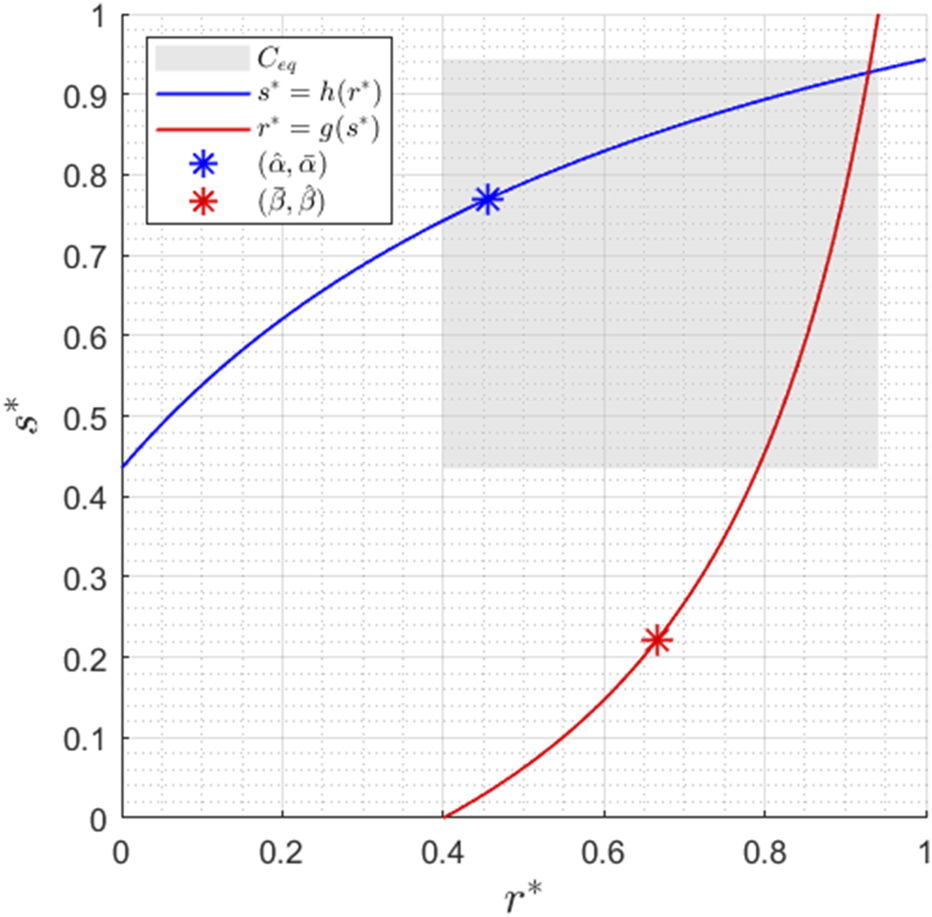
Figure 2. Nullclines for ${\alpha }_1=0.5$, ${\alpha }_2=1$, ${\alpha }_3=1$, ${\alpha }_4=7$, ${\beta }_1=0.3$, ${\beta }_2=1$, ${\beta }_3=1$, ${\beta }_4=4$, $R_T=1$, and $S_T=1$. The $C_{eq}$ region corresponds to the subregion where the equilibrium point is located, as detailed in Proposition 2.

From expression 11, it is easy to obtain ${\mathbb{s}}^{*}=g^{-1}({\mathbb{r}}^{*})$:

$g^{-1}\left({\mathbb{r}}^{*}\right)=\frac{\left({\alpha }_1+{\alpha }_2+{\alpha }_3{S}_T\right){\mathbb{r}}^{*}-{\alpha }_2}{{\alpha }_4{S}_T\left(1-{\mathbb{r}}^{*}\right)+{\alpha }_3{S}_T{\mathbb{r}}^{*}}(13)$

We define the function $\mathrm{\Delta }({\mathbb{r}}^{*})≔h({\mathbb{r}}^{*})-g^{-1}({\mathbb{r}}^{*})$ and note that, by the way $\mathrm{\Delta }({\mathbb{r}}^{*})$ has been defined, if $\left({\mathbb{r}}_{eq}^{*},{\mathbb{s}}_{eq}^{*}\right)$ is an equilibrium point, then $\mathrm{\Delta }({\mathbb{r}}_{eq}^{*})=0$; vice versa, if $\mathrm{\Delta }({\bar{\mathbb{r}}}^{*})=0$ then $\left({\bar{\mathbb{r}}}^{*},h({\bar{\mathbb{r}}}^{*})\right)=\left({\mathbb{r}}_{eq}^{*},{\mathbb{s}}_{eq}^{*}\right)$ is an equilibrium point. It is a matter of computation to verify that $\mathrm{\Delta }({\mathbb{r}}^{*})$ is a rational function—$\mathrm{\Delta }({\mathbb{r}}^{*})=\frac{n({\mathbb{r}}^{*})}{d({\mathbb{r}}^{*})}$—and that both the numerator and denominator are polynomials of order 2:

$\begin{array}{ll}\hfill n\left({\mathbb{r}}^{*}\right)=& \left({\beta }_4{R}_T{\mathbb{r}}^{*}+{\beta }_2\right)\left({\alpha }_4{S}_T\left(1-{\mathbb{r}}^{*}\right)+{\alpha }_3{S}_T{\mathbb{r}}^{*}\right)\hfill \\ \hfill & +-\left({\beta }_1+{\beta }_2+{\beta }_3{R}_T\left(1-{\mathbb{r}}^{*}\right)+{\beta }_4{R}_T{\mathbb{r}}^{*}\right)\hfill \\ \hfill & \times \left(\left({\alpha }_1+{\alpha }_2+{\alpha }_3{S}_T\right){\mathbb{r}}^{*}-{\alpha }_2\right)\hfill \end{array}$

$\begin{array}{ll}\hfill d\left({\mathbb{r}}^{*}\right)& =\left({\beta }_1+{\beta }_2+{\beta }_3{R}_T\left(1-{\mathbb{r}}^{*}\right)+{\beta }_4{R}_T{\mathbb{r}}^{*}\right)\left({\alpha }_4{S}_T\left(1-{\mathbb{r}}^{*}\right)+{\alpha }_3{S}_T{\mathbb{r}}^{*}\right)\hfill \end{array}$

Note that $d({\mathbb{r}}^{*})>0$ for every ${\mathbb{r}}^{*}\in [\mathrm{0,1}]$, and hence $\mathrm{\Delta }({\mathbb{r}}^{*})=0$ for some ${\mathbb{r}}^{*}\in [\mathrm{0,1}]$ if and only if $n({\mathbb{r}}^{*})=0$ for some ${\mathbb{r}}^{*}\in [\mathrm{0,1}]$. Since $n(0)>0$ and $n(1)<0$, there certainly exists ${\mathbb{r}}_{eq}^{*}\in [\mathrm{0,1}]$ such that $n({\mathbb{r}}_{eq}^{*})=0$, and hence $\mathrm{\Delta }({\mathbb{r}}_{eq}^{*})=0$—as already demonstrated, the system admits at least one equilibrium point in $\mathcal{C}$. On the other hand, since $n({\mathbb{r}}^{*})$ is a second-order polynomial, such an ${\mathbb{r}}_{eq}^{*}$ belonging to the interval [0,1] is unique—the system admits a unique equilibrium point $\mathcal{C}$.

Remark 1. Remark 1. A closed-form expression for the equilibrium point of the TCS can be computed as the unique root in interval [0,1] of the second-order polynomial $n({\mathbb{r}}^{*})$.

$\begin{array}{ll}\hfill {\mathbb{r}}_{eq}^{*}& ={\alpha }_3{\beta }_3{R}_T{S}_T-{\alpha }_4{\beta }_4{R}_T{S}_T\pm \hfill \\ \hfill & \frac{\sqrt{A}}{\left(2\left({\alpha }_3{\beta }_3{R}_T{S}_T-{\alpha }_4{\beta }_4{R}_T{S}_T+{\alpha }_1{\beta }_3{R}_T+{\alpha }_2{\beta }_3{R}_T-{\alpha }_1{\beta }_4{R}_T-{\alpha }_2{\beta }_4{R}_T\right)\right)}\hfill \end{array}$

with. $\begin{array}{l}\hfill A=(-{\alpha }_3{\beta }_3{R}_T{S}_T+{\alpha }_4{\beta }_4{R}_T{S}_T-{\alpha }_1{\beta }_3{R}_T-2{\alpha }_2{\beta }_3{R}_T+{\alpha }_2{\beta }_4{R}_T-{\alpha }_3{\beta }_1{S}_T-{\alpha }_4{\beta }_2{S}_T\\ {-{\alpha }_1{\beta }_1-{\alpha }_2{\beta }_1-{\alpha }_1{\beta }_2-{\alpha }_2{\beta }_2)}^2-4({\alpha }_2{\beta }_3{R}_T+{\alpha }_4{\beta }_2{S}_T+{\alpha }_2{\beta }_1+{\alpha }_2{\beta }_2)\hfill \\ ({\alpha }_3{\beta }_3{R}_T{S}_T-{\alpha }_4{\beta }_4{R}_T{S}_T+{\alpha }_1{\beta }_3{R}_T+{\alpha }_2{\beta }_3{R}_T-{\alpha }_1{\beta }_4{R}_T-{\alpha }_2{\beta }_4{R}_T\hfill \\ )+{\alpha }_1{\beta }_3{R}_T+2{\alpha }_2{\beta }_3{R}_T-{\alpha }_2{\beta }_4{R}_T+{\alpha }_3{\beta }_1{S}_T\hfill \\ +{\alpha }_4{\beta }_2{S}_T+{\alpha }_1{\beta }_1+{\alpha }_2{\beta }_1+{\alpha }_1{\beta }_2+\left.{\alpha }_2{\beta }_2\right)\hfill \end{array}$

Proposition 1 states that all trajectories with initial conditions in $\mathcal{C}$ converge to a unique equilibrium point $\left({\mathbb{r}}_{eq}^{*},{\mathbb{s}}_{eq}^{*}\right)\in \mathcal{C}$. This means that, independently of the initial relative amounts of phosphorylated and unphosphorylated proteins, the proportion of phosphorylated to total $RR$ will asymptotically equal ${\mathbb{r}}_{eq}^{*}$, while the proportion of phosphorylated to total $SHK$ will asymptotically tend to ${\mathbb{s}}_{eq}^{*}$. The following proposition identifies a subregion ${\mathcal{C}}_{eq}⊊\mathcal{C}$ where the equilibrium point is located and hence provides upper and lower bounds to the phosphorylation levels ${\mathbb{r}}_{eq}^{*}$ and ${\mathbb{s}}_{eq}^{*}$ asymptotically reached by the TCS.

Proposition 2. Consider the TCS described by models Equations 9, 10. The unique equilibrium point of the system, denoted by $\left({\mathbb{r}}_{eq}^{*},{\mathbb{s}}_{eq}^{*}\right)$, belongs to the subregion

${\mathcal{C}}_{eq}≔\left\{\left({\mathbb{r}}^{*},{\mathbb{s}}^{*}\right):{\mathbb{r}}_{\mathit{min}}^{*}\le {\mathbb{r}}^{*}\le {\mathbb{r}}_{\mathit{max}}^{*},{\mathbb{s}}_{\mathit{min}}^{*}\le {\mathbb{s}}^{*}\le {\mathbb{s}}_{\mathit{max}}^{*}\right\}⊊\mathcal{C},$

where

$\begin{array}{llll}\hfill {\mathbb{r}}_{\mathit{min}}^{*}:& =\frac{{\alpha }_2}{{\alpha }_1+{\alpha }_2+{\alpha }_3{S}_T},\hfill & \hfill {\mathbb{r}}_{\mathit{max}}^{*}:& =\frac{{\alpha }_4{S}_T+{\alpha }_2}{{\alpha }_1+{\alpha }_2+{\alpha }_4{S}_T},\hfill \\ \hfill {\mathbb{s}}_{\mathit{min}}^{*}:& =\frac{{\beta }_2}{{\beta }_1+{\beta }_2+{\beta }_3{R}_T},\hfill & \hfill {\mathbb{s}}_{\mathit{max}}^{*}:& =\frac{{\beta }_4{R}_T+{\beta }_2}{{\beta }_1+{\beta }_2+{\beta }_4{R}_T}\hfill \end{array}$

Proof. Consider the expression for $RR$ nullcline Equation 11 and note that

$\frac{\partial g}{\partial {\mathbb{s}}^{*}}\left({\mathbb{s}}^{*}\right)=\frac{S_T\left({\alpha }_1{\alpha }_4+{\alpha }_4{\alpha }_3{S}_T+{\alpha }_2{\alpha }_3\right)}{{\left({\alpha }_1+{\alpha }_2+{\alpha }_3{S}_T\left(1-{\mathbb{s}}^{*}\right)+{\alpha }_4{S}_T{\mathbb{s}}^{*}\right)}^2}>0\text{for\hspace{0.17em}every}{\mathbb{s}}^{*}\in \left[\mathrm{0,1}\right],$

and hence ${\mathbb{r}}^{*}$ is strictly monotonically increasing in ${\mathbb{s}}^{*}$. The bounds on ${\mathbb{r}}_{eq}^{*}$ then follow from

$g\left(0\right)=\frac{{\alpha }_2}{{\alpha }_1+{\alpha }_2+{\alpha }_3{S}_T}≕{\mathbb{r}}_{\mathit{min}}^{*},\text{and}g\left(1\right)=\frac{{\alpha }_4{S}_T+{\alpha }_2}{{\alpha }_1+{\alpha }_2+{\alpha }_4{S}_T}≕{\mathbb{r}}_{\mathit{max}}^{*},$

Analogous computations on $SHK$ nullcline Equation 12 lead to upper and lower bounds on ${\mathbb{s}}_{eq}^{*}$.

The set ${\mathcal{C}}_{eq}$ is reported in Figure 2 for the set of parameters considered. We conclude this section with the following Lemma, which will be useful for subsequent derivations (see again Figure 2).

Lemma 1. Consider the TCS described by models Equations 9, 10, and define

$\begin{array}{llll}\hfill \bar{\alpha }:& =\frac{{\alpha }_2{\alpha }_3}{{\alpha }_2{\alpha }_3+{\alpha }_1{\alpha }_4}\hfill & \hfill \widehat{\alpha }:& =\frac{{\alpha }_2}{{\alpha }_1+{\alpha }_2}\hfill \\ \hfill \bar{\beta }:& =\frac{{\beta }_2{\beta }_3}{{\beta }_2{\beta }_3+{\beta }_1{\beta }_4}\hfill & \hfill \widehat{\beta }:& =\frac{{\beta }_2}{{\beta }_1+{\beta }_2}\hfill \end{array}$

Then, $RR$ nullcline Equation 11 always passes through $(\bar{\alpha },\widehat{\alpha })$—$g(\bar{\alpha })=\widehat{\alpha }$—while $SHK$ nullcline Equation 12 always passes through $(\bar{\beta },\widehat{\beta })$—$h(\bar{\beta })=\widehat{\beta }$.

This behavior can also be observed in Figure 3, where the dotted lines indicate the nullclines associated with higher values of $R_T$ and $S_T$, while the dashed lines are the nullclines obtained with lower values of $R_T$ and $S_T$, as described in the caption.

Figure 3

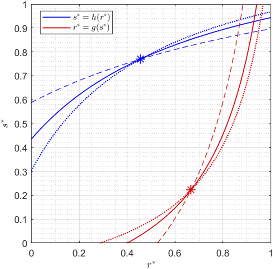
Figure 3. Nullclines for ${\alpha }_1=0.5$, ${\alpha }_2=1$, ${\alpha }_3=1$, ${\alpha }_4=7$, ${\beta }_1=0.3$, ${\beta }_2=1$, ${\beta }_3=1$, and ${\beta }_4=4$. The solid lines have $R_T=1$ and $S_T=1$ as in Figure 2; the dashed lines are obtained with $R_T=0.4$ and $S_T=0.4$; the dotted lines with $R_T=2$ and $S_T=2$.

Since verifying that $g(\bar{\alpha })=\widehat{\alpha }$ and $h(\bar{\beta })=\widehat{\beta }$ is just a matter of computation, the proof of Lemma 1 is omitted.

At this point, two observations are in order. First, the dimensionless values ${\mathbb{r}}_{eq}^{*}$ and ${\mathbb{s}}_{eq}^{*}$ depend on the total amounts of $RR$ and $SHK$ proteins present within the system (recall that, due to time scale separation, so far we have assumed that the quantities $R_T$ and $S_T$ are constant). In other words, ${\mathbb{r}}_{eq}^{*}$ and ${\mathbb{s}}_{eq}^{*}$ are continuous functions of $R_T$ and $S_T$—${\mathbb{r}}_{eq}^{*}={\mathbb{r}}_{eq}^{*}(R_T,S_T)$ and ${\mathbb{s}}_{eq}^{*}={\mathbb{s}}_{eq}^{*}(R_T,S_T)$. The second observation is that uniform monotonicity of ${\mathbb{r}}_{eq}^{*}(R_T,S_T)$ and ${\mathbb{s}}_{eq}^{*}(R_T,S_T)$ with respect to their arguments is not guaranteed. Depending on the values taken by the system parameters, equilibrium ${\mathbb{r}}_{eq}^{*}$ might decrease with $R_T$ when $R_T$ belongs to a specific interval, and increase with $R_T$ when it belongs to a different interval.

3 Relative concentrations

3.1 Low vs high $R_T$ concentration

In this section, we assume that $R_T$ and $S_T$ are independent.

Proposition 3. (Low $R_T$ concentration.) Consider the TCS described by models Equations 9, 10 and let the total $SHK$ concentration $S_T$ be arbitrary but fixed. When the total $RR$ concentration is extremely low—that is, for $R_T\to 0$—the equilibrium point asymptotically reached by the system is given by $\left({\mathbb{r}}_{eq}^{*},{\mathbb{s}}_{eq}^{*}\right)=(g(\widehat{\beta }),\widehat{\beta })$.

Proof. By taking the limit for $R_T\to 0$ of the function $h({\mathbb{r}}^{*})$ defined in Equation 12 and representing $SHK$ nullcline,³ it can be seen that ${\mathbb{s}}_{eq}^{*}=\widehat{\beta }$. The result then follows by plugging ${\mathbb{s}}_{eq}^{*}$ into $RR$-nullcine Equation 11.

Proposition 4. (High $R_T$ concentration.) Consider the TCS described by models Equations 9, 10 and let the total $SHK$ concentration $S_T$ be arbitrary but fixed. When the total $RR$ concentration is extremely high—that is, for $R_T\to +\infty$—the equilibrium point asymptotically reached by the system is $\left({\mathbb{r}}_{hR}^{*},h({\mathbb{r}}_{hR}^{*})\right)$, with ${\mathbb{r}}_{hR}^{*}$ being the (unique) solution in the interval [0,1] of the quadratic equation $\mathbf{A}{({\mathbb{r}}^{*})}^2+\mathbf{B}{\mathbb{r}}^{*}+\mathbf{C}=0$, where

$\begin{array}{ll}\hfill \mathbf{A}:& =\left({\alpha }_1+{\alpha }_2+{\alpha }_3{S}_T\right){\beta }_3-\left({\alpha }_2+{\alpha }_4{S}_T\right){\beta }_4-{\alpha }_1{\beta }_4\hfill \\ \hfill \mathbf{B}:& =-\left({\alpha }_1+{\alpha }_2+{\alpha }_3{S}_T\right){\beta }_3+\left({\alpha }_2+{\alpha }_4{S}_T\right){\beta }_4-{\alpha }_2{\beta }_3\hfill \\ \hfill \mathbf{C}:& ={\alpha }_2{\beta }_3\hfill \end{array}$

More specifically, ${\mathbb{r}}_{hR}^{*}=\left(-\mathbf{B}-\sqrt{{\mathbf{B}}^2-4\mathbf{A}\mathbf{C}}\right)/\left(2\mathbf{A}\right)$.

Proof. Note that when $R_T\to +\infty$, the upper and lower bounds on ${\mathbb{s}}_{eq}^{*}$ are given by ${\mathbb{s}}_{\mathit{min}}^{*}=0$ and ${\mathbb{s}}_{\mathit{max}}^{*}=1$, respectively, and hence do not provide any useful information. Taking the limit for $R_T\to +\infty$ of $RR$ and $SHK$ nullclines Equations 13, 12 yields

$\begin{array}{ll}\hfill \underset{R_T\to +\infty }{\lim }{g}^{-1}\left({\mathbb{r}}^{*}\right)& =\frac{\left({\alpha }_1+{\alpha }_2+{\alpha }_3{S}_T\right){\mathbb{r}}^{*}-{\alpha }_2}{{\alpha }_4{S}_T\left(1-{\mathbb{r}}^{*}\right)+{\alpha }_3{S}_T{\mathbb{r}}^{*}}\hfill \\ \hfill \underset{R_T\to +\infty }{\lim }h\left({\mathbb{r}}^{*}\right)& =\frac{{\beta }_4{\mathbb{r}}^{*}}{{\beta }_4{\mathbb{r}}^{*}+{\beta }_3\left(1-{\mathbb{r}}^{*}\right)}\hfill \end{array}$

Solving for ${\lim }_{R_T\to +\infty }{g}^{-1}({\mathbb{r}}^{*})={\lim }_{R_T\to +\infty }h({\mathbb{r}}^{*})$ leads to the quadratic equation $\mathbf{A}{({\mathbb{r}}^{*})}^2+\mathbf{B}{\mathbb{r}}^{*}+\mathbf{C}=0$. The result now follows upon noting that if $\left({\alpha }_1+{\alpha }_2+{\alpha }_3{S}_T\right){\beta }_3>\left({\alpha }_1+{\alpha }_2+{\alpha }_4{S}_T\right){\beta }_4$, then $\mathbf{A}>0$ and $\mathbf{B}<0$, otherwise $\mathbf{A}<0$; by Descartes’ rule of signs, the quadratic equation has a unique positive solution.

Corollary 1. Consider the TCS described by models Equations 9, 10 and let the total $SHK$ concentration $S_T$ be arbitrary but fixed. Assuming the total $RR$ concentration to be very high—that is, $R_T\to +\infty$—then if ${\beta }_3\ne 0$ and ${\beta }_4=0$, the equilibrium point asymptotically reached by the system is $\left({\mathbb{r}}_{\mathit{min}}^{*},0\right)$; if ${\beta }_3=0$ and ${\beta }_4\ne 0$, the equilibrium point is $\left({\mathbb{r}}_{\mathit{max}}^{*},1\right)$.

Proof. Consider the scenario with ${\beta }_3\ne 0$ and ${\beta }_4=0$ and note that in this case, ${\mathbb{s}}_{\mathit{max}}^{*}=\frac{{\beta }_2}{{\beta }_1+{\beta }_2}$. Taking the limit for $R_T\to +\infty$ of $SHK$ nullcline (12) yields

${\mathbb{s}}_{eq}^{*}=\underset{R_T\to +\infty }{\lim }\frac{{\beta }_2}{{\beta }_1+{\beta }_2+{\beta }_3{R}_T\left(1-{\mathbb{r}}^{*}\right)}=0,{\mathbb{s}}_{\mathit{min}}^{*}=0.$

Then, from $RR$ nullcline Equation 11, we have ${\mathbb{r}}_{eq}^{*}=g({\mathbb{s}}_{eq}^{*})={\mathbb{r}}_{\mathit{min}}^{*}$⁴. The proof for the case ${\beta }_3=0$ and ${\beta }_4\ne 0$ follows the same line and is hence omitted.

Figure 4 reports, for an illustrative set of parameters, equilibrium values ${\mathbb{r}}_{eq}^{*}$ and ${\mathbb{s}}_{eq}^{*}$ as a function of $R_T$.

Figure 4

Figure 4. Equilibrium values ${\mathbb{r}}_{eq}^{*}$ and ${\mathbb{s}}_{eq}^{*}$ continuously depend on the total amount of $RR$ protein $R_T$. Parameter values: ${\alpha }_1=0.5$, ${\alpha }_2=1$, ${\alpha }_3=1$, ${\alpha }_4=7$, ${\beta }_1=0.3$, ${\beta }_2=1$, ${\beta }_3=1$, ${\beta }_4=4$, and $S_T=1$.

By symmetry, analogous results on the equilibrium point hold when the $SHK$ total amount is extremely low or extremely high—$S_T\to 0$ or $S_T\to +\infty$.

3.2 Uniform monotonicity of the equilibrium with respect to $R_T$ and $S_T$

We now consider small perturbations of $R_T$ and $S_T$ concentrations and investigate their effects on the equilibrium point $\left({\mathbb{r}}_{eq}^{*},{\mathbb{s}}_{eq}^{*}\right)$.

We assume first that $S_T$ is constant and consider small perturbations of $R_T$. The equilibrium values continuously depend on $R_T$—that is, $\left({\mathbb{r}}_{eq}^{*},{\mathbb{s}}_{eq}^{*}\right)=\left(g\left({\mathbb{s}}_{eq}^{*},R_T\right),h({\mathbb{r}}_{eq}^{*},R_T)\right)$—and this dependence is quantitatively described by

$\frac{\partial {\mathbb{r}}_{eq}^{*}}{\partial R_T}=\frac{\partial g}{\partial {\mathbb{s}}^{*}}\frac{\partial {\mathbb{s}}_{eq}^{*}}{\partial R_T}(14)$

$\frac{\partial {\mathbb{s}}_{eq}^{*}}{\partial R_T}=\frac{\partial h}{\partial {\mathbb{r}}^{*}}\frac{\partial {\mathbb{r}}_{eq}^{*}}{\partial R_T}+\frac{\partial h}{\partial R_T}(15)$

Conversely, if we assume that total concentration $R_T$ is constant while $S_T$ slowly varies, we have

$\frac{\partial {\mathbb{r}}_{eq}^{*}}{\partial S_T}=\frac{\partial g}{\partial {\mathbb{s}}^{*}}\frac{\partial {\mathbb{s}}_{eq}^{*}}{\partial S_T}+\frac{\partial g}{\partial S_T}(16)$

$\frac{\partial {\mathbb{s}}_{eq}^{*}}{\partial S_T}=\frac{\partial h}{\partial {\mathbb{r}}^{*}}\frac{\partial {\mathbb{r}}_{eq}^{*}}{\partial S_T}(17)$

Putting together Equations 14–17 and solving for the variation of equilibria with respect to $R_T$ and $S_T$, we obtain

$\frac{\partial {\mathbb{r}}_{eq}^{*}}{\partial R_T}=\frac{\frac{\partial h}{\partial R_T}\frac{\partial g}{\partial {\mathbb{s}}^{*}}}{1-\frac{\partial h}{\partial {\mathbb{r}}^{*}}\frac{\partial g}{\partial {\mathbb{s}}^{*}}}\frac{\partial {\mathbb{s}}_{eq}^{*}}{\partial R_T}=\frac{\frac{\partial h}{\partial R_T}}{1-\frac{\partial h}{\partial {\mathbb{r}}^{*}}\frac{\partial g}{\partial {\mathbb{s}}^{*}}}(18)$

$\frac{\partial {\mathbb{r}}_{eq}^{*}}{\partial S_T}=\frac{\frac{\partial g}{\partial S_T}}{1-\frac{\partial h}{\partial {\mathbb{r}}^{*}}\frac{\partial g}{\partial {\mathbb{s}}^{*}}}\frac{\partial {\mathbb{s}}_{eq}^{*}}{\partial S_T}=\frac{\frac{\partial g}{\partial S_T}\frac{\partial h}{\partial {\mathbb{r}}^{*}}}{1-\frac{\partial h}{\partial {\mathbb{r}}^{*}}\frac{\partial g}{\partial {\mathbb{s}}^{*}}}(19)$

Proposition 5. Consider the TCS described by model Equations 9, 10, and let $\left({\mathbb{r}}_{eq}^{*},{\mathbb{s}}_{eq}^{*}\right)$ denote the (unique) equilibrium point of the system. The equilibrium values ${\mathbb{r}}_{eq}^{*}={\mathbb{r}}_{eq}^{*}(R_T,S_T)$ and ${\mathbb{s}}_{eq}^{*}={\mathbb{s}}_{eq}^{*}(R_T,S_T)$ are:

i) monotonically increasing in their arguments if $\widehat{\alpha }>\bar{\beta }$ and $\widehat{\beta }>\bar{\alpha }$;

ii) monotonically decreasing in their arguments if $\widehat{\alpha }<\bar{\beta }$ and $\widehat{\beta }<\bar{\alpha }$.

Proof. Observe that

$\frac{\partial h}{\partial {\mathbb{r}}^{*}}=\frac{R_T\left({\beta }_1{\beta }_4+{\beta }_4{\beta }_3{R}_T+{\beta }_3{\beta }_2\right)}{{\left({\beta }_1+{\beta }_2+{\beta }_3{R}_T\left(1-{\mathbb{r}}^{*}\right)+{\beta }_4{R}_T{\mathbb{r}}^{*}\right)}^2}\ge 0\text{for\hspace{0.17em}every\hspace{0.17em}}{\mathbb{r}}^{*}\in \left[\mathrm{0,1}\right],$

and by symmetry, also $\frac{\partial g}{\partial {\mathbb{s}}^{*}}\ge 0$ for every ${\mathbb{s}}^{*}\in [\mathrm{0,1}]$. Moreover, recall that the function $\mathrm{\Delta }({\mathbb{r}}^{*})≔h({\mathbb{r}}^{*})-g^{-1}({\mathbb{r}}^{*})$ is such that $\mathrm{\Delta }(0)>0$ and $\mathrm{\Delta }(1)<0$ (see proof of Theorem 1), and hence at the equilibrium $\frac{\partial \mathrm{\Delta }}{\partial {\mathbb{r}}^{*}}=\frac{\partial h}{\partial {\mathbb{r}}^{*}}-\frac{\partial g^{-1}}{\partial {\mathbb{r}}^{*}}<0$—$\frac{\partial h}{\partial {\mathbb{r}}^{*}}<\frac{\partial g^{-1}}{\partial {\mathbb{r}}^{*}}$. This, in turn, implies that

$0<\frac{\frac{\partial h}{\partial {\mathbb{r}}^{*}}}{\frac{\partial g^{-1}}{\partial {\mathbb{r}}^{*}}}=\frac{\partial h}{\partial {\mathbb{r}}^{*}}\frac{\partial g}{\partial {\mathbb{s}}^{*}}<1$

Then, the sign of the partial derivatives Equations 18, 19 are solely determined by $\frac{\partial h}{\partial R_T}$ and $\frac{\partial g}{\partial S_T}$ since all other terms are always non-negative. It is a matter of computation to verify that

$\frac{\partial h}{\partial R_T}=\frac{\left({\beta }_1{\beta }_4+{\beta }_2{\beta }_3\right){\mathbb{r}}^{*}-{\beta }_2{\beta }_3}{{\left({\beta }_1+{\beta }_2+{\beta }_3{R}_T\left(1-{\mathbb{r}}^{*}\right)+{\beta }_4{R}_T{\mathbb{r}}^{*}\right)}^2},$

and hence at equilibrium $\mathrm{s}\mathrm{i}\mathrm{g}\mathrm{n}\left(\frac{\partial h}{\partial R_T}\right)=\mathrm{s}\mathrm{i}\mathrm{g}\mathrm{n}({\mathbb{r}}_{eq}^{*}-\bar{\beta })$. Exploiting again the symmetry of the system, we can claim that $\mathrm{s}\mathrm{i}\mathrm{g}\mathrm{n}\left(\frac{\partial g}{\partial S_T}\right)=\mathrm{s}\mathrm{i}\mathrm{g}\mathrm{n}({\mathbb{s}}_{eq}^{*}-\bar{\alpha })$. Hence, provided that ${\mathbb{r}}_{eq}^{*}$ $({\mathbb{s}}_{eq}^{*})$ is greater than $\bar{\beta }$ (respectively, $\bar{\alpha }$), both ${\mathbb{r}}_{eq}^{*}$ and ${\mathbb{s}}_{eq}^{*}$ are monotonically increasing functions of $R_T$ (respectively, $S_T$). Similarly, provided that ${\mathbb{r}}_{eq}^{*}$ $({\mathbb{s}}_{eq}^{*})$ is smaller than $\bar{\beta }$ (respectively, $\bar{\alpha }$), both ${\mathbb{r}}_{eq}^{*}$ and ${\mathbb{s}}_{eq}^{*}$ are monotonically decreasing functions of $R_T$ (respectively, $S_T$). It is clear from Figure 2 that when $\widehat{\alpha }>\bar{\beta }$ and $\widehat{\beta }>\bar{\alpha }$, the equilibrium values necessarily satisfy the inequalities ${\mathbb{r}}_{eq}^{*}>\bar{\beta }$ and ${\mathbb{s}}_{eq}^{*}>\bar{\alpha }$, and the thesis follows.

Remark 2. The conditions on the system parameters provided by proposition 5 are sufficient (but not necessary) for uniform monotonicity of the equilibrium concerning total concentrations $R_T$ and $S_T$. It is worth noticing that such a result is extremely powerful; its strength resides in the fact that it does not depend on the specific form of the functions $R_T$ and $S_T$ (provided they are monotone). More specifically, let $R_T=f_R(u_{\mathit{ext}})$ and $S_T=f_S(u_{\mathit{ext}})$, where $u_{\mathit{ext}}$ is an external signal and $f_R$ and $f_S$ are monotone functions. Then, $u_{\mathit{ext}}=f_R^{-1}(R_T)$, and the relationship between $S_T$ and $R_T$ is given by $S_T=f_S◦f_R^{-1}(R_T)$ (note that the composite function $f_S◦f_R$ is itself monotone). Proposition 5 states that if $\widehat{\alpha }>\bar{\beta }$ and $\widehat{\beta }>\bar{\alpha }$, monotonicity of the equilibrium with respect to $R_T$ and $S_T$ is ensured independently on the specific form of the monotone functions $f_R$ and $f_S$. If the previous conditions are not satisfied, uniform monotonicity is not guaranteed.

We now focus on the case where a proportionality relationship among $R_T$ and $S_T$ can be assumed: $S_T=f_S◦f_R(R_T)=\lambda R_T$. Note that this is a perfectly reasonable assumption when phosphorylated $RR$ activates the transcription of both its gene and the gene encoding its partner $SHK$—see, for example, the mathematical description of the MprA/MprB two-component system adopted in (Tiwari et al., 2010).

Theorem 1. Consider the TCS described by models Equations 9, 10, and assume that total $RR$ and $SHK$ concentrations are related by $S_T=\lambda R_T$, where $\lambda >0$ is a fixed (not necessarily known) proportionality coefficient. When the total $RR$ concentration is extremely high—that is, for $R_T\to +\infty$—the (unique) equilibrium point asymptotically reached by the system is

$\left({\mathbb{r}}_{eq}^{*},{\mathbb{s}}_{eq}^{*}\right)=\left\{\begin{array}{cc}\left(\mathrm{0,0}\right),\hfill & \text{if}\frac{{\alpha }_3{\beta }_3}{{\alpha }_4{\beta }_4}>1\hfill \\ \left(\mathrm{1,1}\right),\hfill & \text{if}\frac{{\alpha }_3{\beta }_3}{{\alpha }_4{\beta }_4}<1\hfill \end{array}\right.$

Proof. Compute the limit for $R_T\to +\infty$ of $RR$ and $SHK$ nullclines Equations 11, 12:

${\mathbb{r}}^{*}=\underset{R_T\to +\infty }{\lim }g\left({\mathbb{s}}^{*},\lambda R_T\right)=\frac{{\alpha }_4{\mathbb{s}}^{*}}{{\alpha }_3+\left({\alpha }_4-{\alpha }_3\right){\mathbb{s}}^{*}},\text{for\hspace{0.17em}every\hspace{0.17em}}\lambda >0(20)$

${\mathbb{s}}^{*}=\underset{R_T\to +\infty }{\lim }h\left({\mathbb{r}}^{*},R_T\right)=\frac{{\beta }_4{\mathbb{r}}^{*}}{{\beta }_3+\left({\beta }_4-{\beta }_3\right){\mathbb{r}}^{*}}(21)$

From expression Equation 21, it is easy to obtain

${\mathbb{r}}^{*}=h^{-1}\left({\mathbb{s}}^{*}\right)=\frac{{\beta }_3{\mathbb{s}}^{*}}{{\beta }_4+\left({\beta }_3-{\beta }_4\right){\mathbb{s}}^{*}}$

Substituting the previous expression into Equation 20 and solving for ${\mathbb{s}}^{*}$ yields the following quadratic equation:

${\left({\mathbb{s}}^{*}\right)}^2\left\{\left({\alpha }_4{\beta }_4-{\alpha }_3{\beta }_3\right){\mathbb{s}}^{*}+\left({\alpha }_3{\beta }_3-{\alpha }_4{\beta }_4\right)\right\}=0$

Then, the only two possible equilibrium points are $({\mathbb{r}}_{eq}^{*},{\mathbb{s}}_{eq}^{*})=(\mathrm{0,0})$ and $({\mathbb{r}}_{eq}^{*},{\mathbb{s}}_{eq}^{*})=(\mathrm{1,1})$. To determine which is the right solution, we need to resort to the intersection condition $\frac{\partial h}{\partial {\mathbb{r}}^{*}}\frac{\partial g}{\partial {\mathbb{s}}^{*}}<1$ (see the proof of Proposition 5). Indeed, it is straightforward to verify that

$\begin{array}{ll}\hfill \underset{R_T\to +\infty }{\lim }\frac{\partial h}{\partial {\mathbb{r}}^{*}}& =\frac{{\beta }_3{\beta }_4}{{\left({\beta }_3+\left({\beta }_4-{\beta }_3\right){\mathbb{r}}^{*}\right)}^2}\hfill \\ \hfill \underset{R_T\to +\infty }{\lim }\frac{\partial g}{\partial {\mathbb{s}}^{*}}& =\frac{{\alpha }_3{\alpha }_4}{{\left({\alpha }_3+\left({\alpha }_4-{\alpha }_3\right){\mathbb{s}}^{*}\right)}^2},\hfill \end{array}$

and hence

$\begin{array}{ll}\hfill \frac{\partial h}{\partial {\mathbb{r}}^{*}}\frac{\partial g}{\partial {\mathbb{s}}^{*}}{|}_{({\mathbb{r}}^{*},{\mathbb{s}}^{*})=(\mathrm{0,0})}& =\frac{{\beta }_4}{{\beta }_3}\frac{{\alpha }_4}{{\alpha }_3}\hfill \\ \hfill \frac{\partial h}{\partial {\mathbb{r}}^{*}}\frac{\partial g}{\partial {\mathbb{s}}^{*}}{|}_{({\mathbb{r}}^{*},{\mathbb{s}}^{*})=(\mathrm{1,1})}& =\frac{{\beta }_3}{{\beta }_4}\frac{{\alpha }_3}{{\alpha }_4},\hfill \end{array}$

which uniquely determines the limiting equilibrium pair once the quantity $\frac{{\beta }_4}{{\beta }_3}\frac{{\alpha }_4}{{\alpha }_3}$ is known.

Remark 3. The previous result does not require knowledge of the value assumed by the proportionality coefficient $\lambda$; we just need to know that a proportionality coefficient continuously relates $R_T$ and $S_T$

4 Absolute concentrations

We have thus far analyzed the properties (asymptotic behavior and monotonicity) of relative concentrations: of the ratio between phosphorylated and unphosphorylated protein concentrations. A fundamental and crucial point is that these properties do not necessarily hold for absolute concentrations too: the fact that the relative concentration ${\mathbb{r}}_{eq}^{*}$ tending to 0 does not imply that absolute concentration $r_{eq}^{*}$ tends to 0; similarly, uniform monotonicity of ${\mathbb{r}}_{eq}^{*}$ for $R_T$ does not imply uniform monotonicity of $r^{*}$ to $R_T$. To understand this point, note that the relative concentration ${\mathbb{r}}_{eq}^{*}$ tends to 0 when total $RR$ concentration asymptotically grows to infinity (i.e., $R_T\to +\infty$) and $r^{*}$ asymptotically approaches a given saturation level $r_{eq}^{*}\ne 0$. Regarding monotonicity, since $r^{*}={\mathbb{r}}^{*}{R}_T$, it holds that

$\frac{\partial r^{*}}{\partial R_T}=\frac{\partial {\mathbb{r}}^{*}}{\partial R_T}{R}_T+{\mathbb{r}}^{*}$

It is clear that if ${\mathbb{r}}_{eq}^{*}$ is a monotonically increasing function of $R_T$ (namely, $\frac{\partial {\mathbb{r}}^{*}}{\partial R_T}>0$), so is $r_{eq}^{*}$. On the contrary, if ${\mathbb{r}}_{eq}^{*}$ is a monotonically decreasing function of $R_T$, and hence $\frac{\partial {\mathbb{r}}^{*}}{\partial R_T}<0$; monotonicity of $r_{eq}^{*}$ with respect to $R_T$ is not guaranteed.

In the following, we analyze the asymptotic behavior of absolute concentrations $r_{eq}^{*}$ and $s_{eq}^{*}$ when $R_T$ grows to infinity, under the assumption that $RR$ and $SHK$ total concentrations are linearly related with the proportionality coefficient $\lambda$—$S_T=\lambda R_T$.

Theorem 2. Consider the TCS described by models Equations 9, 10 and assume that the total $RR$ and $SHK$ concentrations are linearly related by $S_T=\lambda R_T$, where $\lambda >0$ is a fixed proportionality coefficient. When total $RR$ concentration is sufficiently high—that is, for $R_T\to +\infty$, $RR$ and $SHK$—then absolute concentrations asymptotically approach the equilibrium values:

$\begin{array}{ll}\hfill r_{eq}^{*}& =\frac{{\alpha }_2{\beta }_3+\lambda {\alpha }_4{\beta }_2}{\lambda \left({\alpha }_3{\beta }_3-{\alpha }_4{\beta }_4\right)}\hfill \\ \hfill s_{eq}^{*}& =\frac{{\alpha }_2{\beta }_4+\lambda {\alpha }_3{\beta }_2}{{\alpha }_3{\beta }_3-{\alpha }_4{\beta }_4},\hfill \end{array}$

respectively.

Proof. We claim that for a sufficiently high $R_T$, absolute equilibrium concentrations $r_{eq}^{*}$ and $s_{eq}^{*}$ asymptotically approach saturation levels $\mathrm{\rho }$ and $\mathrm{\sigma }$:

$\begin{array}{ll}\hfill \underset{R_T\to +\infty }{\lim }\left\{{\mathbb{r}}_{eq}^{*}\left(R_T,\lambda R_T\right)\cdot R_T\right\}& =\mathrm{\rho },\hfill \\ \hfill \underset{R_T\to +\infty }{\lim }\left\{{\mathbb{s}}_{eq}^{*}\left(R_T,\lambda R_T\right)\cdot \lambda R_T\right\}& =\mathrm{\sigma }\hfill \end{array}$

We now seek to determine the values $\mathrm{\rho }$ and $\mathrm{\sigma }$. First, we note that

$\begin{array}{ll}\hfill \mathrm{\rho }& =\underset{R_T\to +\infty }{\lim }g\left({\mathbb{s}}_{eq}^{*}\left(R_T,\lambda R_T\right),\lambda R_T\right)\cdot R_T\hfill \\ \hfill & =\underset{R_T\to +\infty }{\lim }\frac{{\alpha }_4\lambda R_T{\mathbb{s}}_{eq}^{*}\left(R_T,\lambda R_T\right)+{\alpha }_2}{{\alpha }_1+{\alpha }_2+{\alpha }_3\lambda R_T\left(1-{\mathbb{s}}_{eq}^{*}\left(R_T,\lambda R_T\right)\right)+{\alpha }_4\lambda R_T{\mathbb{s}}_{eq}^{*}\left(R_T,\lambda R_T\right)}\cdot R_T\hfill \\ \hfill & =\underset{R_T\to +\infty }{\lim }\frac{{\alpha }_4\mathrm{\sigma }+{\alpha }_2}{{\alpha }_1+{\alpha }_2+{\alpha }_3\lambda R_T+\left({\alpha }_4-{\alpha }_3\right)\mathrm{\sigma }}\cdot R_T\hfill \\ \hfill & =\frac{{\alpha }_4\mathrm{\sigma }+{\alpha }_2}{\lambda {\alpha }_3}\hfill \end{array}$

Analogously, the limit of $s_{eq}^{*}$ for $R_T\to +\infty$ can be computed as

$\begin{array}{ll}\hfill \mathrm{\sigma }& =\underset{R_T\to +\infty }{\lim }h\left({\mathbb{r}}_{eq}^{*}\left(R_T,\lambda R_T\right),\lambda R_T\right)\cdot \lambda R_T\hfill \\ \hfill & =\underset{R_T\to +\infty }{\lim }\frac{{\beta }_4{R}_T{\mathbb{r}}_{eq}^{*}\left(R_T,\lambda R_T\right)+{\beta }_2}{{\beta }_1+{\beta }_2+{\beta }_3{R}_T\left(1-{\mathbb{r}}_{eq}^{*}\left(R_T,\lambda R_T\right)\right)+{\beta }_4{R}_T{\mathbb{r}}_{eq}^{*}\left(R_T,\lambda R_T\right)}\cdot \lambda R_T\hfill \\ \hfill & =\underset{R_T\to +\infty }{\lim }\frac{{\beta }_4\mathrm{\rho }+{\beta }_2}{{\beta }_1+{\beta }_2+{\beta }_3{R}_T+\left({\beta }_4-{\beta }_3\right)\mathrm{\rho }}\cdot \lambda R_T\hfill \\ \hfill & =\frac{\left({\beta }_4\mathrm{\rho }+{\beta }_2\right)\lambda }{{\beta }_3}\hfill \end{array}$

Therefore, we need to solve the linear system:

$\left\{\begin{array}{c}\mathrm{\rho }\lambda {\alpha }_3={\alpha }_4\mathrm{\sigma }+{\alpha }_2\hfill \\ \mathrm{\sigma }{\beta }_3=\left({\beta }_4\mathrm{\rho }+{\beta }_2\right)\lambda \hfill \end{array}\right.$

Solving for $\mathrm{\rho }$ and $\mathrm{\sigma }$ yields

$\mathrm{\rho }=\frac{{\alpha }_2{\beta }_3+\lambda {\alpha }_4{\beta }_2}{\lambda \left({\alpha }_3{\beta }_3-{\alpha }_4{\beta }_4\right)},\mathrm{\sigma }=\frac{{\alpha }_2{\beta }_4+\lambda {\alpha }_3{\beta }_2}{{\alpha }_3{\beta }_3-{\alpha }_4{\beta }_4},$

Thus, the proof is concluded.

It follows from Theorem 2 that for sufficiently high $R_T$, while the amount of phosphorylated $SHK$ increases with $\lambda$, the amount of phosphorylated $RR$ is a decreasing function of $\lambda$, such that

$r_{eq}^{*}=\frac{\frac{1}{\lambda }{\alpha }_2{\beta }_3+{\alpha }_4{\beta }_2}{{\alpha }_3{\beta }_3-{\alpha }_4{\beta }_4}(22)$

5 Discussion

A distinguishing feature of the proposed TCS mathematical model is that it accounts for a variety of reactions, including $RR$ phosphorylation and dephosphorylation through external (exogenous) pathways, $SHK$ autophosphorylation and autodephosphorylation, $RR$ phosphorylation via phosphotransfer from $SHK$, and $RR$ dephosphorylation via $SHK$. Of course, by setting 0 for one or more parameters, the model can be tailored to specific two-component systems (TCSs) and/or situations in which some of the previous reactions are negligible.

One of the best characterized examples of TCS is the EnvZ/OmpR system in Escherichia coli, which responds to changes in environmental osmolality by regulating the expression of the outer membrane porins OmpF and OmpC. As in many TCSs, EnvZ is a bifunctional sensor histidine kinase, meaning that it phosphorylates and dephosphorylates the response regulator OmpR. Batchelor and Goulian (2003) proposed a mathematical model of the EnvZ/OmpR TCS and experimentally tested the model’s predictions. Their main finding was that for sufficiently high amounts of OmpR, when total EnvZ in the cell is much less abundant than total OmpR⁵, the steady-state level of phosphorylated OmpR is robust (insensitive) to fluctuations in EnvZ and OmpR concentrations. This model accounts for the autokinase, phosphotransfer, and phosphatase activities of EnvZ and neglects the exogenous phosphorylation and dephosphorylation of OmpR. Casting such a scenario into our mathematical framework means setting ${\alpha }_2$ and ${\beta }_4$ to 0. Theorem 2 then implies that the equilibrium absolute concentration for OmpR is given by $r_{eq}^{*}=\frac{{\alpha }_4{\beta }_2}{{\alpha }_3{\beta }_3}$, and hence, consistent with Batchelor and Goulian (2003), does not depend on EnvZ total concentration. However, our model shows that if an exogenous $RR$ phosphorylation flux is present (${\alpha }_2\ne 0$), the previous result fails; when an external pathway for OmpR phosphorylation is present, the steady-state concentration of phosphorylated OmpR is (higher and) decreasing with $\lambda$ (see Equation 22). Notably, Batchelor and Goulian (2003) predicted, via theoretical analysis and experimental verification with fluorescent reporter strains, that when condition $S_T\ll R_T$ does not hold, the steady-state value of OmpR-P decreases with increasing total EnvZ concentration. This is consistent with our theoretical results, which also shed light on the role of an EnvZ-independent mechanism for OmpR phosphorylation.

Furthermore, our analysis allows the characterization of the steady-state concentration of the histidine kinase: $s_{eq}^{*}=\lambda \frac{{\beta }_2}{{\beta }_3}$ (recall that ${\beta }_4=0$). As expected, our model predicts that the amount of phosphorylated EnvZ increases with more vigorous autokinase activity $({\beta }_2)$ and decreases with stronger phosphotransfer activity of the histidine kinase $({\beta }_3)$.

Finally, while our analysis demonstrates the existence of a single robust equilibrium of the system (Theorem 1), it is instructive to consider the possibility of using such a building block as part of a closed-loop system with positive retroactivity, which could lead to oscillatory or bistable behaviors (Igoshin et al., 2008; Zorzan et al., 2021; Tiwari et al., 2010).

5.1 Phosphotransfer and reverse phosphotransfer reactions

Bifunctional sensor histidine kinase exerts both positive and negative control through $SHK$ phosphotransfer and phosphatase activity, respectively. While the biochemical reactions underlying $SHK$ kinase activity are reasonably well understood, the mechanisms of phosphatase activity represent a long-standing question, the investigation of which has led to the formulation of multiple hypotheses (see Huynh and Stewart, 2011 for an overview). An early hypothesis, first proposed by Dutta and Inouye (1996), identified reverse transfer of the phosphoryl group from phosphorylated $RR$ to $SHK$ as a potential $RR$ dephosphorylation mechanism. Such a hypothesis was prompted by experimental results conducted on EnvZ/OmpR system in E. coli (Dutta and Inouye, 1996; Zhu et al., 2000), showing that reverse transfer of the phosphoryl group from OmpR-P to EnvZ was detected in the early period of the phosphatase reaction with domain A of EnvZ—specifically with the EnvZ ${\text{kinase}}^{-}$ ${\text{phosphatase}}^{+}$ mutant (EnvZ.N347D), and, under certain conditions, with the wild-type EnvZ.

Even if later experiments invalidated the reverse phosphotransfer model (Hsing and Silhavy, 1997), it is universally recognized that reverse phosphotransfer can occur under certain conditions. As pointed out by Gao and Stock (2009), multiple mechanisms may have evolved for phosphatase activities, and individual histidine kinases may utilize different regulatory strategies. We now aim to theoretically investigate a scenario in which both direct and reverse phosphotransfer reactions occur, and a distinct phosphatase activity of the sensor histidine is present.

Since the kinase activity of $SHK$ takes the form of a phosphotransfer reaction (by which a phosphoryl group is transferred from phosphorylated $SHK$ to $RR$), reaction rates ${\alpha }_4$ and ${\beta }_3$ are actually equal—${\alpha }_4={\beta }_3$. We first assume that only $SHK$ exhibits phosphotransfer activity (${\beta }_4=0$), and we rename ${\alpha }_3$ as ${\alpha }_3^p$, where superscript $p$ stands for “phosphatase activity” (of the $SHK$). It follows from Theorem 2 that when total $RR$ concentration is sufficiently high, steady-state absolute concentrations are given by ${\mathbb{r}}_{eq}^{*}=\frac{\frac{1}{\lambda }{\alpha }_2+{\beta }_2}{{\alpha }_3^p}$ and $s_{eq}^{*}=\lambda \frac{{\beta }_2}{{\beta }_3}$.

When reverse phosphotransfer from phosphorylated $RR$ to $SHK$ occurs, the reaction rate ${\beta }_4$ is non-zero and ${\alpha }_3={\alpha }_3^p+{\alpha }_3^{rt}$, with ${\alpha }_3^{rt}={\beta }_4$ (where superscript $rt$ stands for “reverse phosphotransfer”). Then, recalling that ${\alpha }_4={\beta }_3$, Theorem 2 yields

$r_{eq}^{*}=\frac{\frac{1}{\lambda }{\alpha }_2+{\beta }_2}{{\alpha }_3^p}\text{\hspace{0.17em}and\hspace{0.17em}}{s}_{eq}^{*}=\lambda \frac{{\beta }_2}{{\beta }_3}+\frac{{\alpha }_2{\beta }_4+\lambda {\alpha }_3^{rt}{\beta }_2}{{\alpha }_3^p{\beta }_3}=\lambda \frac{{\beta }_2}{{\beta }_3}+\frac{{\alpha }_3^{rt}\left({\alpha }_2+\lambda {\beta }_2\right)}{{\alpha }_3^p{\beta }_3}$

This indicates that, even if reverse phosphotransfer occurs, the absolute concentration of phosphorylated $RR$ remains unchanged. While this may seem contradictory at first, it is easily explained by noting that reverse phosphotransfer from phosphorylated $RR$ to $SHK$ is exactly compensated by the increased direct phosphotransfer from phosphorylated $SHK$ to $RR$. On the contrary, when the reverse phosphotransfer reaction occurs, our analysis shows that the absolute concentration of $SHK$ increases and that such an increase is larger for higher values of the reverse phosphotransfer rate (bigger ${\alpha }_3^{rt}$) and/or for larger amounts of total $SHK$ concentration (bigger $\lambda$).

This study’s main findings are summarized here in comparison with the literature.

6 Conclusion

We here developed a generalized mathematical model for bacterial two-component signaling systems that integrates canonical phosphorylation cycles, bifunctional enzymatic activities, transcriptional feedback, and potential auxiliary interactions. Through systems-level analysis, we elucidated how network architecture and parameter regimes shape key dynamic properties and robustness.

Our modeling framework provides a predictive foundation for interpreting experimental dynamics, as illustrated for the EnvZ/OmpR system, and for guiding the rational design of synthetic signaling circuits. We demonstrated that the bifunctionality of the sensor histidine kinase, multi-step phosphorelays, and transcriptional feedback, which are incorporated into the model, enable rich behaviors that allow TCSs to precisely tune cellular responses to diverse environmental stimuli.

Notably, we derived analytical conditions in Propositions 3, Propositions 4, Propositions 5 and Theorem 1 under which the steady-state levels of phosphorylated proteins exhibit input–output robustness, overshoot, or bistability. We also characterized in Sections 3–4 how the equilibrium phosphorylation levels depend on the absolute and relative abundances of the two components. These insights are critical for understanding natural mechanisms of bacterial adaptation and for forward-engineering synthetic gene circuits with prescribed dynamics.

By combining the mechanistic modeling framework with systems analysis techniques, such as nullcline analysis, this study provides a unified perspective on the structural design principles that underlie the remarkable versatility of two-component signal transduction. The proposed generalized model lays a theoretical foundation for further experimental investigations, such as exploring reverse phosphotransfer mechanisms, and establishes a framework for rationally harnessing two-component systems in synthetic biology applications.

Data availability statement

The original contributions presented in the study are included in the article/supplementary material; further inquiries can be directed to the corresponding author.

Author contributions

IZ: Writing – original draft, Methodology, Formal Analysis, Investigation, Conceptualization, Visualization. CC: Methodology, Writing – review and editing, Formal Analysis, Visualization. LS: Funding acquisition, Resources, Supervision, Methodology, Writing – original draft, Conceptualization. MB: Visualization, Project administration, Investigation, Supervision, Writing – review and editing.

Funding

The author(s) declare that no financial support was received for the research and/or publication of this article.

Conflict of interest

The authors declare that the research was conducted in the absence of any commercial or financial relationships that could be construed as a potential conflict of interest.

Generative AI statement

The author(s) declare that no Generative AI was used in the creation of this manuscript.

Any alternative text (alt text) provided alongside figures in this article has been generated by Frontiers with the support of artificial intelligence and reasonable efforts have been made to ensure accuracy, including review by the authors wherever possible. If you identify any issues, please contact us.

Publisher’s note

All claims expressed in this article are solely those of the authors and do not necessarily represent those of their affiliated organizations, or those of the publisher, the editors and the reviewers. Any product that may be evaluated in this article, or claim that may be made by its manufacturer, is not guaranteed or endorsed by the publisher.

Footnotes

¹Actually, in (Tiwari et al., 2010) production of $RR$ and $SHK$ is described by the summation of two activating Hill functions. As explained later, since we are focusing on the functioning of the Two-Component System, the separation of time scales allows us to assume constant production rates.

²Since every limit cycle is a closed orbit, ruling out the existence of closed orbits automatically excludes the existence of limit cycles.

³An equivalent way to see that ${\mathbb{s}}_{eq}^{*}=\widehat{\beta }$ when $R_T\to 0$ is noticing that in this case both ${\mathbb{s}}_{\mathit{min}}^{*}$ and ${\mathbb{s}}_{\mathit{max}}^{*}$ tend to ${\beta }_2/\left({\beta }_1+{\beta }_2\right)=\widehat{\beta }$, and hence the subregion ${\mathcal{C}}_{eq}$ reduces to a line.

⁴Alternatively, the result directly follows from Proposition 4 with ${\beta }_3=0$.

⁵As reported, for instance, in (Hsing and Silhavy, 1997), in vivo OmpR is nearly 100-fold more abundant than EnvZ.

References

Alvarez, A. F., and Georgellis, D. (2023). Environmental adaptation and diversification of bacterial two-component systems. Curr. Opin. Microbiol. 76, 102399. doi:10.1016/j.mib.2023.102399

PubMed Abstract | CrossRef Full Text | Google Scholar

Batchelor, E., and Goulian, M. (2003). “Robustness and the cycle of phosphorylation and dephosphorylation in a two-component regulatory system,”, 100. Proceedings of the National Academy of Sciences, (Washington, D.C., USA: National Academy of Sciences), 691–696. doi:10.1073/pnas.0234782100

CrossRef Full Text | Google Scholar

Blanchini, F., and Miani, S. (2015). Set-theoretic methods in control systems and control: Foundations and applications. Basel, Switzerland: Birkhäuser Basel.

Google Scholar

Dutta, R., and Inouye, M. (1996). Reverse phosphotransfer from OmpR to EnvZ in a kinase-/phosphatase+ mutant of EnvZ (EnvZ.N347D), a bifunctional signal transducer of Escherichia coli. J. Biol. Chem. 271, 1424–1429. doi:10.1074/jbc.271.3.1424

PubMed Abstract | CrossRef Full Text | Google Scholar

Gao, R., and Stock, A. (2009). Biological insights from structures of two-component proteins. Annu. Rev. Microbiol. 63, 133–154. doi:10.1146/annurev.micro.091208.073214

PubMed Abstract | CrossRef Full Text | Google Scholar

Goulian, M. (2010). Two-component signaling circuit structure and properties. Curr. Opin. Microbiol. 13, 184–189. doi:10.1016/j.mib.2010.01.009

PubMed Abstract | CrossRef Full Text | Google Scholar

Groisman, E. (2016). Feedback control of two-component regulatory systems. Annu. Rev. Microbiol. 70, 103–124. doi:10.1146/annurev-micro-102215-095331

PubMed Abstract | CrossRef Full Text | Google Scholar

Hsing, W., and Silhavy, T. (1997). Function of conserved histidine-243 in phosphatase activity of EnvZ, the sensor for porin osmoregulation in Escherichia coli. J. Bacteriol. 179, 3729–3735. doi:10.1128/jb.179.11.3729-3735.1997

PubMed Abstract | CrossRef Full Text | Google Scholar

Huynh, T., and Stewart, V. (2011). Negative control in two-component signal transduction by transmitter phosphatase activity. Mol. Microbiol. 82, 275–286. doi:10.1111/j.1365-2958.2011.07829.x

PubMed Abstract | CrossRef Full Text | Google Scholar

Igoshin, O., Alves, R., and Savageau, M. (2008). Hysteretic and graded responses in bacterial two-component signal transduction. Mol. Microbiol. 68, 1196–1215. doi:10.1111/j.1365-2958.2008.06221.x

PubMed Abstract | CrossRef Full Text | Google Scholar

Kirby, J. R. (2009). Chemotaxis-like regulatory systems: unique roles in diverse bacteria. Annu. Rev. Microbiol. 63, 45–59. doi:10.1146/annurev.micro.091208.073221

PubMed Abstract | CrossRef Full Text | Google Scholar

Mitrophanov, A., Hadley, T., and Groisman, E. (2010). Positive autoregulation shapes response timing and intensity in two-component signal transduction systems. J. Mol. Biol. 401, 671–680. doi:10.1016/j.jmb.2010.06.051

PubMed Abstract | CrossRef Full Text | Google Scholar

Mukherji, S., and van Oudenaarden, A. (2009). Synthetic biology: understanding biological design from synthetic circuits. Nat. Rev. Genet. 10, 859–871. doi:10.1038/nrg2697

PubMed Abstract | CrossRef Full Text | Google Scholar

Müller, M. M., Arndt, K. M., and Hoffmann, S. A. (2025). Genetic circuits in synthetic biology: broadening the toolbox of regulatory devices. Front. Synthetic Biol. 3, 1548572. doi:10.3389/fsybi.2025.1548572

CrossRef Full Text | Google Scholar

Pasotti, L., Bellato, M., Casanova, M., Zucca, S., Cusella De Angelis, M. G., and Magni, P. (2017). Re-using biological devices: a model-aided analysis of interconnected transcriptional cascades designed from the bottom-up. J. Biol. Eng. 11, 50. doi:10.1186/s13036-017-0090-3

PubMed Abstract | CrossRef Full Text | Google Scholar

Ramos, A. L., Aquino, M., García, G., Gaspar, M., de la Cruz, C., Saavedra-Flores, A., et al. (2022). Rpus/r is a novel two-component signal transduction system that regulates the expression of the pyruvate symporter mctp in Sinorhizobium fredii ngr234. Front. Microbiol. 13, 871077. doi:10.3389/fmicb.2022.871077

PubMed Abstract | CrossRef Full Text | Google Scholar

Rao, S., and Igoshin, O. (2021). Overlaid positive and negative feedback loops shape dynamical properties of phopq two-component system. PLoS Comput. Biol. 17, e1008130. doi:10.1371/journal.pcbi.1008130

PubMed Abstract | CrossRef Full Text | Google Scholar

Ray, J., and Igoshin, O. (2010). Adaptable functionality of transcriptional feedback in bacterial two-component systems. PLOS Comput. Biol. 6, e1000676–10. doi:10.1371/journal.pcbi.1000676

PubMed Abstract | CrossRef Full Text | Google Scholar

Sastry, S. (1999). Nonlinear systems. Analysis, stability, and control. Interdiscip. Appl. Math. 10. doi:10.1007/978-1-4757-3108-8

CrossRef Full Text | Google Scholar

Shinar, G., Milo, R., Martínez, M., and Alon, U. (2007). “Input-output robustness in simple bacterial signaling systems,”, 104. Proceedings of the National Academy of Sciences, (Washington, D.C., USA: National Academy of Sciences), 19931–19935. doi:10.1073/pnas.0706792104

CrossRef Full Text | Google Scholar

Stock, A., Robinson, V., and Goudreau, P. (2000). Two-component signal transduction. Annu. Rev. Biochem. 69, 183–215. doi:10.1146/annurev.biochem.69.1.183

PubMed Abstract | CrossRef Full Text | Google Scholar

Tierney, A. R., and Rather, P. N. (2019). Roles of two-component regulatory systems in antibiotic resistance. Future Microbiol. 14, 533–552. doi:10.2217/fmb-2019-0002

PubMed Abstract | CrossRef Full Text | Google Scholar

Tiwari, A., Balazsi, G., Gennaro, M., and Igoshin, O. (2010). The interplay of multiple feedback loops with post-translational kinetics results in bistability of mycobacterial stress response. Phys. Biol. 7, 036005. doi:10.1088/1478-3975/7/3/036005

PubMed Abstract | CrossRef Full Text | Google Scholar

Tiwari, S., Jamal, S. B., Hassan, S. S., Carvalho, PVSD, Almeida, S., Barh, D., et al. (2017). Two-component signal transduction systems of pathogenic bacteria as targets for antimicrobial therapy: an overview. Front. Microbiol. 8, 1878. doi:10.3389/fmicb.2017.01878

PubMed Abstract | CrossRef Full Text | Google Scholar

Zhu, Y., Qin, L., Yoshida, T., and Inouye, M. (2000). Phosphatase activity of histidine kinase EnvZ without kinase catalytic domain. Proc. Natl. Acad. Sci. 97, 7808–7813. doi:10.1073/pnas.97.14.7808

PubMed Abstract | CrossRef Full Text | Google Scholar

Zorzan, I., Del Favero, S., Giaretta, A., Manganelli, R., Di Camillo, B., and Schenato, L. (2021). Mathematical modelling of sige regulatory network reveals new insights into bistability of mycobacterial stress response. BMC Bioinforma. 22, 558. doi:10.1186/s12859-021-04372-5

PubMed Abstract | CrossRef Full Text | Google Scholar

Zschiedrich, C., Keidel, V., and Szurmant, H. (2016). Molecular mechanisms of two-component signal transduction. J. Mol. Biol. 428, 3752–3775. doi:10.1016/j.jmb.2016.08.003

PubMed Abstract | CrossRef Full Text | Google Scholar