 Julian Koch
 Jane Gotfredsen
 Raphael Schneider
 Simon Stisen
 Hans Jørgen Henriksen
- Department of Hydrology, Geological Survey of Denmark and Greenland, Copenhagen, Denmark
Detailed knowledge of the uppermost water table representing the shallow groundwater system is critical in order to address societal challenges that relate to the mitigation and adaptation to climate change and enhancing climate resilience in general. Machine learning (ML) allows for high resolution modeling of the water table depth beyond the capabilities of conventional numerical physically-based hydrological models with respect to spatial resolution and overall accuracy. For this, in-situ well and proxy observations are used as training data in combination with high resolution covariates. The objective of this study is to model the depth of the uppermost water table for a typical summer and winter condition at 10 m spatial resolution over entire Denmark (43,000 km2). CatBoost, a state of the art implementation of gradient boosting decision trees, is employed in this study to model the water table depth and the associated uncertainties. The groundwater domain has not been the most prominent field of applications of recent hydrological ML advances due to the lack of big data. This study brings forward a novel knowledge-guided ML framework to overcome this limitation by integrating simulation results from a physically-based groundwater flow model. The simulation data are utilized to (1) identify wells that represent the uppermost water table, (2) augment missing training data by accounting for simulated water level seasonality, and (3) expand the list of covariates. The curated training dataset contains around 13,000 wells, 19,000 groundwater proxy observations at lakes, streams and coastline as well as 15 covariates. Cross validation attests that the ML model generalizes well with a mean absolute error of around 115 cm considering solely well observations and a MAE of <50 cm taking also the proxy observations into consideration. Quantile regression is applied to estimate confidence intervals and the estimated uncertainty is largest for moraine clay soils that are characterized with a distinct geological heterogeneity. This study highlights a novel research avenue of knowledge-guided ML for the groundwater domain by efficiently supporting a ML model with a physically-based hydrological model to predict the depth of the water table at unprecedented spatial detail and accuracy.
Introduction
A key state variable of the hydrological cycle is the depth of the uppermost water table, i.e., shallow groundwater, with a broad range of crucial societal, and environmental implications such as securing infrastructure, food production and sustaining ecosystems (Gleeson et al., 2016). Following the global analysis of water table patterns by Fan et al. (2013), up to one-third of the land area is influenced by shallow groundwater, being either directly groundwater-fed or having the water table or capillary fringe within plant rooting depths. More concretely, the shallow groundwater system plays a key role in building mitigation and adaptation measures to address climate change, as the uppermost water table controls greenhouse gas emissions from wetlands (Tiemeyer et al., 2016, 2020) and as rising groundwater exacerbates flooding and falling groundwater intensifies droughts (Taylor et al., 2013). Floods can either be directly induced or intensified by the shallow groundwater system which has a special relevance for urban areas (MacDonald et al., 2012; Bricker et al., 2017). In an agronomical context, the shallow groundwater system is vital to meet crop water requirements in many agricultural settings while having adverse consequences for crop yield when the water table is too close to the surface (Kahlown et al., 2005; Zipper et al., 2015). Moreover, the uppermost water table constitutes a link between subsurface and the land-surface by affecting the energy balance and near-surface climatic conditions (Larsen et al., 2016; Maxwell and Condon, 2016).
The above mentioned relevancy of the shallow groundwater system requires versatile modeling systems to meet the demands of decision makers with respect to accuracy and spatial resolution. Accuracy and spatial resolution can be considered main bottlenecks in the advancement of physically-based numerical hydrological models. Increasing the spatial resolution does not necessarily go along with an improvement of the model accuracy, as established process descriptions and parametrizations are not always scalable (Beven and Cloke, 2012; Clark et al., 2017). At the same time, increasing the number of computational units results in a computational burden limiting the possibility to conduct thorough parameter calibration and sensitivity analysis. Due to the stringent parametrization and rigid model structure, conventional hydrological models cannot fully harness the wealth of readily available environmental big data. Nevertheless, physically-based models integrate decades of hydrological knowledge and are indispensable for integrated assessments of the hydrological cycle and simulating hydrological response under non-stationarity, i.e., climate change. As outlined by Shen (2018), Reichstein et al. (2019), and Nearing et al. (2020), machine learning (ML) is gaining increasing attention in the hydrological science to overcome some of the previously mentioned constraints of conventional physically-based models. ML has the advantage of being data flexible with respect to optimally utilizing the wealth of environmental big data while providing accurate predictions at low computational costs. However, ML lacks process descriptions which commonly restricts trained ML models to deliver predictions within observed ranges of the training dataset. In order to reconcile advantages of both modeling perceptions, knowledge-guided ML forms a promising new research avenue (Rajaee et al., 2019; Kraft et al., 2020). Knowledge-guided ML has the aim to integrate physical consistency into ML improve model performance and robustness. There exist multiple approaches to design knowledge-guided ML models as outlined by Read et al. (2019), Reichstein et al. (2019), Konapala et al. (2020), and others, which are also referred to as physics- or process-guided. A clear formal definition of these modeling approaches is still lacking, but they generally aim at integrating aspects of scientific knowledge into a ML model.
This study aims at modeling the depth of the uppermost water table at 10 m spatial resolution over entire Denmark for a typical summer and winter condition by implementing a knowledge-guided ML model. The physically-based information are obtained from the Danish national water resources model, that integrates groundwater and surface water processes (Højberg et al., 2013; Stisen et al., 2019). The physically-based model is used three-fold, (1) to derive threshold depths to select wells that reflect the shallow groundwater, (2) to augment training data at wells with incomplete pairs of summer-winter observations, and (3) to inform the ML model with the typical summer and winter water table depth using simulation results at 100 m resolution.
Decision tree based ML models are popular tools for geospatial modeling of environmental variables (Hengl et al., 2018; Tyralis et al., 2019b). In this context a target variable, available as point data, is used in conjunction with maps of explanatory variables to curate a training dataset. Relationships between the target variable and the explanatory variables are established via the decision trees which, once trained, can be generalized to make predictions of the target variable at all grids. This framework has been successfully applied across the geosciences to model water chemistry indicators (Tesoriero et al., 2015; Erickson et al., 2021) soil properties (Møller et al., 2017; Hengl et al., 2021), subsurface redox conditions (Close et al., 2016; Koch et al., 2019a), water table depth (Bechtold et al., 2014; Koch et al., 2019b), and other variables. In such modeling frameworks, uncertainty can be quantified via quantile regression (López López et al., 2014; Tyralis et al., 2019a). Gradient boosting is among the state of the art techniques to build decision tree models and, for this study we have employed the CatBoost implementation of gradient boosting decision trees (Dorogush et al., 2018; Prokhorenkova et al., 2018). Numerous studies apply ML to model the temporal water table dynamics by using various ML techniques (Sun et al., 2016; Guzman et al., 2017; Wunsch et al., 2021). These studies highlight successful applications, but are always limited to time series modeling, at a few selected sites. Despite these efforts, the spatial dimension is often neglected in the published studies. Fienen et al. (2013), Bechtold et al. (2014), and Koch et al. (2019b) are among the few studies that model the spatial variability of water table depth using ML. Knowledge-guided ML applications in the groundwater domain are for example the physics informed neural networks model developed by Guo et al. (2020) that allows to solve partial differential equations with less calculational time.
The three main objectives of the paper are as follows: (1) to train a ML model to predict the uppermost water table depth at 10 m spatial resolution over entire Denmark, (2) to quantify uncertainty using quantile regression, and (3) to formalize a knowledge-guided ML framework that builds upon a physically-based hydrological model.
Materials and Methods
Study Area
This study is carried out for the entire land phase of Denmark, located in Northern Europe and covering an area of around 43,000 km2 (Figure 1). Denmark is generally flat with a maximum elevation of 170 m.a.s.l. and agriculture is the main land cover with around 70%. The landscape of Denmark was formed by a sequence of Pleistocene glaciations and postglacial processes. The soils of eastern Denmark are dominated by Weichselian moraine sediments with a moderate clay content, whereas western Denmark is characterized by older moraine sediments originating from the Saalian age intertwined by sandy Weichselian outwash plains.
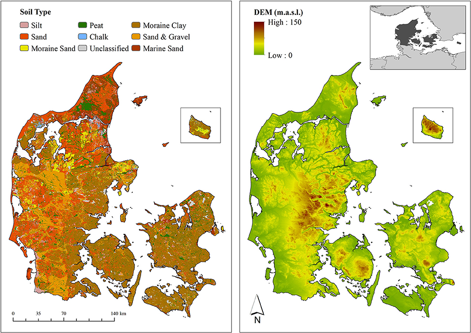
Figure 1. The left panel depicts the soil types of Denmark classified into nine dominant classes (Henriksen et al., 2020). The right panel depicts a digital elevation map of Denmark. The Island Bornholm, located in the Eastern Baltic sea (see overview map), is added as an independent map layer to both panels.
In Denmark, the groundwater system is under pressure as a consequence of climate change and abstractions, revealed by quantitative modeling assessments conducted by Henriksen et al. (2008) and Karlsson et al. (2016). More specifically, a shallow water table rise of up to 1.5 m for a 100-year event relative to present average conditions was estimated by Kidmose et al. (2013) for an urban catchment.
Data
In order to make seasonal estimates (typical winter and typical summer) of the shallow water table at high resolution, an initial comprehensive data processing has been conducted to curate a high-quality dataset containing water level observations at shallow wells, additional groundwater observations as well as national maps of explanatory variables.
Physically-Based Model
The national water resources model of Denmark (DK-model), which has previously been refined from the original 500 m resolution to an updated 100 m resolution, was employed in this study (Højberg et al., 2013; Stisen et al., 2019; Henriksen et al., 2020). The core of the DK-model is an integrated surface-subsurface hydrological model (MIKE SHE model code) that is calibrated against streamflow and groundwater observations. We utilized simulation results of the depth of the uppermost water table at daily time step from a 30 year simulation period (1990–2019) and processed the data to the maps depicted in Figure 2. The summer condition reflects a median across 30 summers, each summer defined as the median of the months June, July, and August. Analogous, the winter condition is based on the median of 30 winters, where each winter is defined as the median of the months December, January, and February of the same winter season. The third processed variable is the simulated median seasonality, which is based on the median across 30 annual seasonalities. For each year, the seasonality has been calculated as median summer condition minus median winter condition. The simulated summer condition has a mean water table depth of 3.5 m whereas the simulated winter condition has a mean of 2.6 m, with a standard deviation of 5.8 and 4.8 m, respectively In terms of the spatial pattern, the simulated water table depth shows overall resemblance between the summer and the winter condition. Deepest groundwater levels are found in the Western part of Denmark alongside high elevation and for sandy soils. The moraine clay soils are characterized with a dominant shallow water table, especially during the winter months. The simulated median seasonality has a mean of 85 cm. The spatial pattern of the simulated seasonality reflects a complex interplay of geology and topography. The amplitude is generally low in topographical sinks and high for areas with an elevated topography. A majority of the moraine clay soils possess an amplitude larger than 1 m, which is caused by a winter water table at the surface due to slow infiltration in combination with a drying out in the summer months.
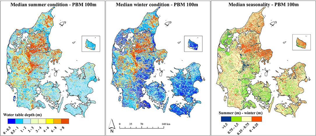
Figure 2. Simulation results for the depth of the uppermost water table from a national physically-based model (PBM) at 100m spatial resolution: The left panel shows the simulated median summer condition (JJA). The center panel shows the simulated median winter condition (DJF). The right panel depicts the median seasonality, calculated as summer minus winter.
Groundwater Observations
The open-access Danish well database (Jupiter) contains around 100,000 wells with at least a single water table observation in the selected 30-year period between 1990 and 2019. Based on the national well dataset, we first identified the wells that represent the shallow groundwater system, i.e., characterize the uppermost water table. Given the geological complexity of Denmark, this can vary from just a few meters for locations with a thick surficial clay layer to several tens of meters for the sandy outwash plains. In order to find suitable threshold depths, that classify a well as being either shallow or not, we combined the national soil map (Figure 1) and the simulated uppermost water table (Figure 2). For this analysis, the midpoint intake depth of each well was used, which is relative to the top and the bottom of the intake. The 95th percentile of the simulated water table depth was calculated for each soil type which guided the definition of the presented threshold depths applied to the midpoint intake depths of the wells (Table 1). Wells were only selected if the intake depth was lower than the soil type dependent threshold depth. A spatially soil type distributed threshold depth, guided by a physically-based model, has the advantage to reflect the natural conditions best possibly. Alternative, a constant threshold depth of e.g., 10 m would result in the selection of wells that do not reflect the uppermost water table in clayey settings where a well may be placed in a sand unit below a 6 m surficial clay layer containing the uppermost water table.
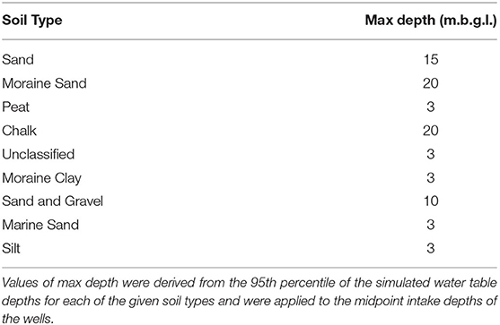
Table 1. Threshold depths that define a shallow well with respect to soil types (Figure 1).
After applying the soil types dependent threshold depths, summer, and winter depths to the uppermost groundwater were calculated at each well. For this task, summer refers to observations from the months June, July, and August (JJA) whereas winter refers to the months December, January, and February (DJF). Inter-annual variation was not considered during this processing step and in case a well contained several summer or winter observations a median was calculated. This resulted in 13,047 well, as shown in Figure 3, of which 1,378 wells had both a summer and a winter observation, 5,651 only a winter observation and 6,018 only a summer observation. For the wells that were missing either a winter or a summer observation the simulated median seasonality (Figure 2) was used to augment the missing season, i.e., winter = summer—seasonality, and vice versa. Further, the training dataset was extended by additional observations that reflect proxy observations for surficial groundwater levels with a depth of zero. In total, 19,074 groundwater connected lakes with an aerial extent of at least 100 m2 were used for this purpose. Additionally, 1,000 points, randomly placed along each, the stream network and along the coastline, were added to better represent these under sampled settings where the water table is expected to be at the surface year-round. This resulted in a total number of 34,061 groundwater observations spread across Denmark, yielding a density of around 0.8 observations per km2. Based on the well data only, the average summer depth is 3.6 and 3.1 m for the winter season with a standard deviation of 2.8 m for both.
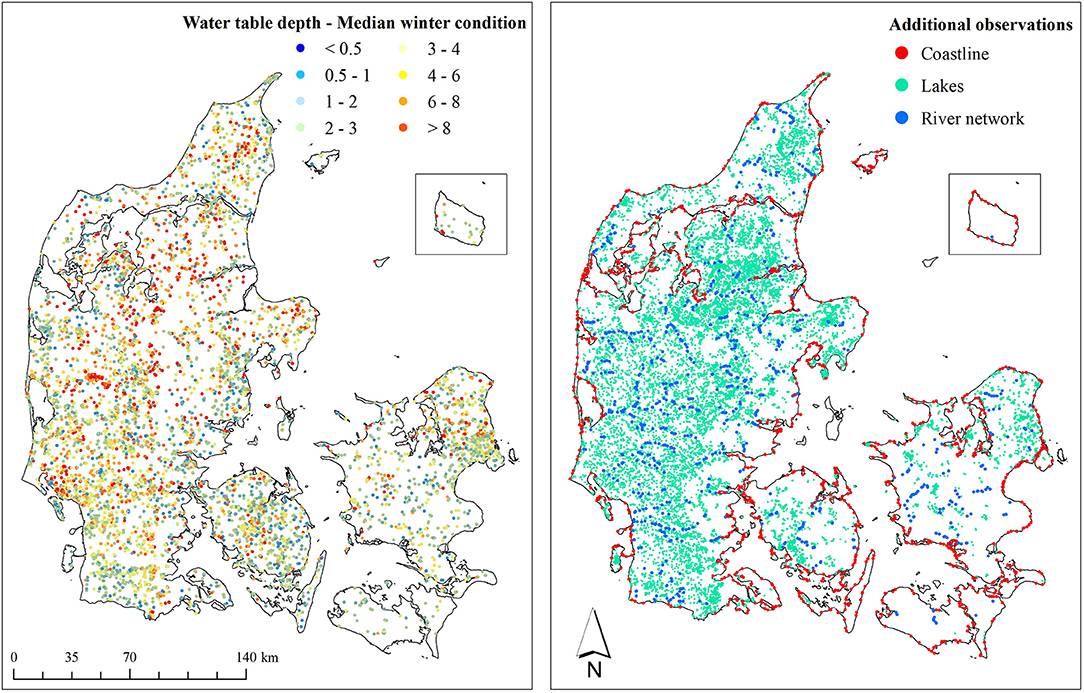
Figure 3. Training dataset containing wells (left panel) and additional observations (right panel). The dataset contains 13,047 shallow wells with both a winter and a summer observation. The additional observations comprise 19,074 groundwater connected lakes, 1,000 stream points and 1,000 coastal points. All additional observations were defined with zero depth of the uppermost water table.
Explanatory Variables
In Table 2, an overview of the covariates used to model the depth of the uppermost water table is presented. In total, 15 covariates were assembled as input to the ML model. This list comprises information on soil texture, geology, topography-based characteristics, water body proximity, land cover, and outputs from a hydrological simulation with the DK-model. The native spatial resolution of the covariates varied, but all covariates were resampled to 10 m to be in agreement with the defined output resolution. For the resampling we used a bilinear interpolation method for the continuous variables. The water body proximity was expressed as both the vertical and horizontal distance to the nearest water body, which contained rivers, lakes, and the coastline.

Table 2. Overview of the explanatory variables used to model the uppermost water table.
Gradient Boosting Decision Trees
We applied a new implementation of the gradient boosting decision tree (GBDT) algorithm, i.e., Cat Boost that was first developed by Yandex engineers in 2017 (Dorogush et al., 2018; Prokhorenkova et al., 2018). GBDT, first introduced by Friedman (2001), is a popular ML method that is increasingly being applied across the geosciences for both, classification, and regression tasks (Fan et al., 2018; Georganos et al., 2018; Møller et al., 2018). GBDT builds a prediction model based on an ensemble of weak learners, i.e., decision trees. In an additive training process, GBDT attempts to correct itself by adding a decision tree trained against the residuals of the ensemble sum of its predecessors for a pre-defined number of iterations. Small incremental steps are taken to correct the residuals, which is controlled via the learning rate. The learning rate is a key hyper parameter of GBDT that is multiplied with the predicted residuals of each decision tree. In order to further alleviate overfitting, stochasticity is added to the training process via subsampling of the training dataset each time a new tree is built. Also, CatBoost allows for early stopping of the training process once the objective function for a test dataset stagnates for a defined number of iterations. The individual decision trees are constrained by a number of hyper parameters, such as tree depth or the minimum number observations per split. CatBoost is specifically designed to work well with categorical variables and a preprocessing of categorical variables by means of different encoding methods is not necessary. Also, CatBoost is favorable over similar ML algorithms, such as Random Forests, Support Vector Machines, or other GBDT implementations (e.g., XGboost or LightGBM), with respect to computational time and memory usage, while achieving a competitive accuracy (Huang et al., 2019; Hancock and Khoshgoftaar, 2020). Given the size of the training dataset (34,061 grids and 15 variables) and the prediction dataset (430 million grids and 15 variables) the memory efficiency and the overall computational time were crucial parameters for the selection of the ML algorithm. The covariate importance of a trained CatBoost model can be revealed through analysis of the tree splits to calculate how much the prediction changes on average if the feature value changes.
For the purpose of simulating the depth of the uppermost water table using CatBoost we employ two different objective functions. First, the mean absolute error (MAE) is used to train the best estimate of the winter and summer condition. One model is trained for each season. The MAE is expressed as follows:
where sim is the simulated groundwater depth and obs the observed for a total of n training data. Besides simulating the best estimate, we are also interested in quantifying the uncertainty of the model. For this, we utilized quantile regression to define objective functions targeting specific quantiles of the distribution. This yields a probabilistic model that is not trained to estimate the conditional mean, but to estimate a defined quantile q of the distribution instead:
Setting q to 0.5 yields the same result as the MAE, but setting q to other values will give asymmetric weights to the residual depending on q and the overall sign of the error. Setting q to 0.1 will estimate the 10th percentile, by associating a weight of 0.9 to over predictions and a weight of 0.1 to under predictions. Thereby the 10th percentile can be approximated, meaning that the model will be trained to over predict 90% of the times. With the uncertainty analysis we intend to estimate the 68 and 95% confidence intervals which can be achieved by training four models, each model targeting a single quantile (e.g., 0.16 and 0.84 for the 68% confidence interval). The four models have to be trained individually for both, summer, and winter condition. We used CPU on a Windows machine (4 2.2 GHz Intel Xeon processors with 56 cores in total, 256 GB RAM) for training and prediction.
Results
High Resolution Groundwater Model
CatBoost regression was used to simulate the depth of the uppermost water table for a typical winter and summer condition at 10 m resolution over entire Denmark. Hyper parameters were first manually calibrated and afterwards automatically fine-tuned using a randomized search approach. Table 3 contains the nine hyper parameters included in the randomized search, a short description, and the tested values. The randomized hyper parameter search was conducted for the summer and the winter model using a 3-fold cross validation approach using 75% of the data. The 3-fold cross validation is the default of CatBoost's randomized hyper parameter search algorithm. The MAE, based on the 2,500 hyper parameter combination derived from the randomized search algorithm, varied just 4 cm. A common hyper parameter set that was among the top 2% for both, summer, and winter model, was selected for further modeling (Table 3). We found that the performance did not deteriorate for the test data (25%).
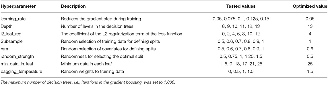
Table 3. CatBoost hyper parameter used in the randomized search (2,500 combinations).
Table 4 shows results obtained from a 4-fold cross validation test for the summer and winter models. For this, four CatBoost regression models were trained using 75% of the data for training and 25% of the data was held back for validation. Overall, little variation was found across the cross validation models, which indicates an overall robustness. The MAE, averaged across the four cross validation test, is 47 cm for both, summer, and winter model. This calculation is based on the entire training dataset. Only considering well data yields an average MAE of around 1.15 m. The increase in MAE is due to the fact that the additional observations, all with a depth of zero, are well-captured by the model and generally yield lower residuals. Based on the coefficient of determination over half of the variance in the well data is accounted for by the models and over 70% of the variance of the entire training dataset. The 19,000 lakes are represented with a MAE of below 5 cm, whereas additional observations along the stream network and coastline possess a MAE of around 10 cm.
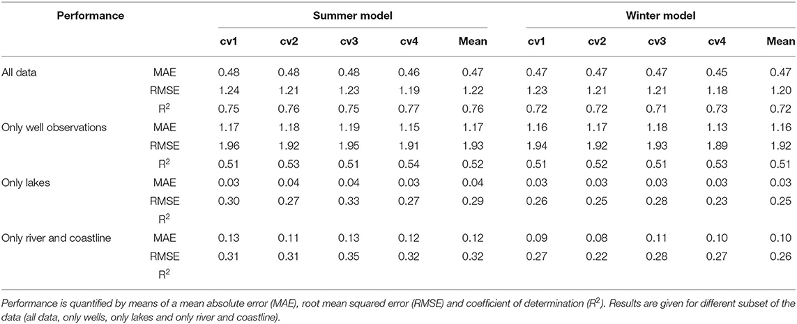
Table 4. Results for a 4-fold cross validation (cv) applied on the summer and winter model.
Figure 4 depicts the simulated national maps of the depth of the uppermost water table at 10 m spatial resolution for summer and winter. The maps offer much detail revealing the interplay of geology, topography, and waterbody proximity. The overall regional patterns show resemblance with the simulations results of the physically-based model at 100 m, which were used as covariate in the 10 m ML models (Figure 2). However, disagreements between the 100 m physically-based model and the 10 m ML model are also present. The former simulates a shallower water table in the Eastern part of Demark where moraine clay is the dominant lithology. This is especially the case for the winter condition. Further, the 100 m physically-based model simulates a homogeneously deep water table in the sandy areas whereas the ML model results in more heterogeneity. The disagreements may be explained by the differences in spatial resolution, but also with the vertical discretization of the computational layers in the physically-based model. Sandy layers quickly run dry which results in a deep water table and clayey layers hold water which yields a very shallow water table. The ML based median seasonality is calculated as the difference between the summer and the winter maps. The amplitude is generally lowest close to streams and lakes and highest in the center of Denmark where topography is high and a permeable subsurface is present. Similar to the physically-based simulated amplitude, the ML derived amplitude has intermediate values around 0.5 m (yellow category) in the Western part of Denmark for the sandy outwash plains. Based on both approaches, the amplitude for the moraine clay settings is around 1 m (green category) which is mainly driven by the very shallow water table during winter.
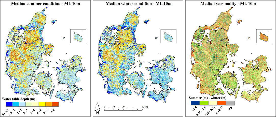
Figure 4. Simulation results for the depth of the uppermost water table obtained from the summer and winter model at 10m spatial resolution, left and center panel, respectively. The right panel depicts the simulated amplitude calculated as summer depth minus winter depth.
Figure 5 presents the same data as shown in Figure 4, just for a zoom section of ~15 km2. Here, the imprint of the stream network as well as the many lakes, become apparent as areas with a very shallow depth of the uppermost water table (< 0.5 m). The difference between the drier summer and the wetter winter is clearly notable and the difference between the two models is plotted as the seasonality. The largest amplitude is present in areas with high topography and the lowest amplitude is found along the river network and lakes.
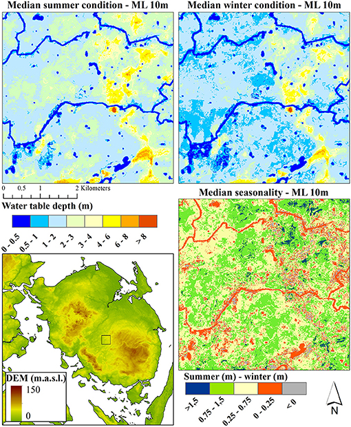
Figure 5. Same data as presented in Figure 4, but zoomed to an ~15 km2 area located on the island of Fyn. The zoom location is indicated in the overview map (bottom left).
Covariate Importance
The quantified importance of each input feature for the summer and winter model is presented in Figure 6 for the entire training dataset and for a subset containing only the well data. Based on a trained model, CatBoost calculates the “prediction value change” to quantify how much on average the prediction changes if the covariate value changes. The average changes that represent the importance of a given covariate are normalized to add up to 100. The vertical distance to the closest water body (VDis) clearly stands out as the most importance covariate in both models. At locations with VDis close to zero, the water table is typically also close to the surface. However, large VDis values, which indicate small scale topographical variations often result in a deeper water level, as the shallow groundwater does not follow the topography in such settings. The most important categorical covariate is the landscape type classification (LType) which contains 13 landscape classes, such as moraine, marine plains, outwash plains, and others. There is little difference between winter and summer model, which indicates robustness between the two models. Differences between covariate importance with respect to the entire dataset and only well data conveys that the horizontal distance to the closest water body (HDis) is mostly relevant to the additional observations, namely lakes, rivers, and coast, which is expectable as these are characterized with a distance of zero. The physically-based model (PBM) stands out as second most important covariate when only considering the well-training dataset. This underlines that the physically-based model can provide the ML model with a meaningful information, despite the differences in spatial resolution, since both model the same variable.
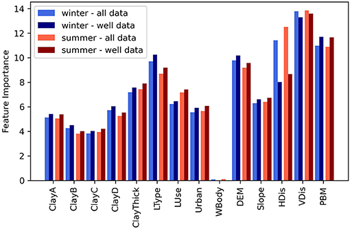
Figure 6. Covariate importance quantified as prediction change in % calculated for summer and winter model for two subsets of training data (all data and well data only). The covariate abbreviations are explained in Table 2.
Uncertainty Analysis
Quantile regression has been applied in order to estimate the uncertainties associated with the summer and winter models. For both models, four quantile models have been trained using the same hyper parameters as applied previously. The quantile models were set with q = 0.16 and 0.84 for the 68% confidence interval and q = 0.025 and 0.975 for the 95% confidence interval. Results are shown in Figure 7 and were calculated on the basis of the same 4-fold cross validation test as presented in Table 4. Figure 7 only contains wells and data are sorted with respect to the simulated groundwater depth and increase alongside an increasing x-axis. The observations, 13,047 in total, are plotted as a density plot and an overall good agreement between model and observations can be attested to both, summer, and winter. The blue envelope plots indicate the two confidence intervals and following the quantile regression definition, 5% of the observations are expected to be outside the light blue envelope (95% confidence) and 32% are expected to be outside the dark blue envelope (68% confidence). For both, the summer, and winter model, the uncertainty increases with depth, which gets supported by the large spread of observations for larger depths. Groundwater depths above 6 m have an uncertainty of around 4 and 8 m following the 68 and 95% confidence intervals.
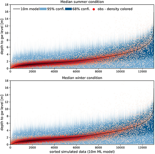
Figure 7. Results of the 4-fold cross validation test for summer model (top) and winter model (bottom). The simulated data are sorted, and the observations are plotted as point density. Only well observations are shown in the plot. Uncertainty bands are included for two confidence intervals.
Based on the 95% confidence interval, which reflects the spread of ~±2 standard deviations around the mean, a map of the standard deviation at 10 m spatial resolution has been calculated. Overall, the relationship between the standard deviation and the water table depth is nearly linear and the coefficient of determination, expressed as the average standard deviation over the average water table depth is 0.58. This indicates that the uncertainty is roughly half of its water table depth value. Figure 8 exemplifies the relationship between the simulated depth of water table and the associated uncertainty (standard deviation) for two soil types. In moraine clay soils, the depth of the uppermost water table is typically in the top few meters, whereas moraine sand soils are characterized with deeper water tables. The coefficient of variation for the two soil types is 0.74 for moraine clay and 0.44 for moraine sand which underlines that uncertainty is larger for moraine clay soils as opposed to moraine sand soils. This can be expected given the distinct geological heterogeneity in the moraine clay soils.
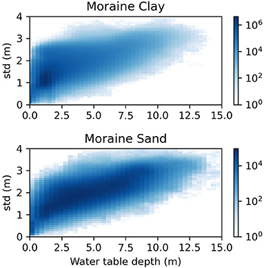
Figure 8. Density scatter plot showing the simulated depth of the groundwater for moraine clay and sand soil against the associated standard deviation (std.) for the winter model. Results are shown for two of the nine soil types (Figure 1).
Discussion
Training Dataset
The winter trainings dataset comprises all DJF water level observations and JJA represents summer conditions. The median was calculated in the case of multiple observations per well per season. This approach introduces uncertainties since it rules out inter-annual variability and further, variability within the summer and winter seasons is also ignored. This compromise was accepted in order to obtain a large trainings dataset of groundwater observations. Large-scale groundwater datasets are typically very heterogenous, which is especially the case for the temporal dimension. The spatial density of wells may be high, but the temporal resolution of water level observations poses challenges to ML applications. Heterogeneity originates from varying frequencies and periods of observations. As an example, around 66% of the 104,000 wells in Denmark have only a single observation in the period of 1990–2019. In order to capitalize on under sampled shallow wells in a big data context, this study brings forward a knowledge-guided ML framework that employs the simulated seasonality from a physically-based groundwater flow model. With this augmentation strategy, the training dataset could be expanded significantly from 1,378 shallow wells with both, summer and winter observations, to 13,047 with either gap-filled summer or winter observation. Previously, Koch et al. (2019b) employed a temporal projection of any given well observation to a representative extreme winter condition using a simple sinusoidal model that was fitted to numerous hydrogeological units. While this approach was purely observational based it was limited to a few pre-defined hydrogeological units whereas the knowledge-guided framework presented herein made use of a spatially distributed groundwater model that provides groundwater amplitudes, i.e., seasonality, at higher spatial detail. Further, the training dataset was extended by groundwater proxy observations featuring lakes, rivers, and coastline where the water table depth is expected to be zero. These information were partly derived from expert knowledge, which is another important aspect of the concept of knowledge-guided ML, which has special relevance for the data-scarce groundwater domain. The simulation results of the physically-based groundwater model were employed to identify wells that are representative for the shallow groundwater system, i.e., representing the uppermost water table, by means of soil type dependent threshold depths. This process step was essential to train the ML against a homogenized well dataset and omitting this would result in a dataset with well observations containing water levels of different aquifer systems.
This study utilized a comprehensive set of 15 covariates to predict water table variability. This selection has been guided by a previous Danish study by Koch et al. (2019b). As an additional covariate, satellite-based radar data, which have shown to be sensitive to shallow water table dynamics within the first couple of meters below surface (Bechtold et al., 2018), could potentially be employed as a meaningful input to the future developments of the framework presented in this study. Other high resolution satellite data on land surface temperature or shortwave infrared (obtained from e.g., Landsat) could provide relevant information to differentiate moisture conditions in areas where land use is constant and the water table is close to the surface.
Temporal Resolution
This study implements a simplified temporal dimension of the groundwater table, by simulating two seasons, namely a typical winter and summer condition. These temporal snapshots are of course a prude simplification of a variable that is known to possess a distinct temporal variability. However, previous studies that apply ML to model the spatial variability of the water table have focused on a single time step; i.e., Koch et al. (2019b) model an extreme wintertime condition and Fienen et al. (2013) and Bechtold et al. (2014) focus on mean annual conditions. ML applications that focus on time series modeling of the water table are typically limited to a few wells with complete time series of daily or monthly observations spanning over several years (Sun et al., 2016; Guzman et al., 2017; Wunsch et al., 2021). Such modeling techniques, which are often based on deep learning due to its strengths in sequence modeling, have not yet been rolled out to model the full spatio-temporal variability of groundwater dynamics due to geological complexity and data scarcity. Full spatio-temporal modeling schemes would require thorough testing on how a dynamic ML model can be transferred from one location to another. This is especially challenging for the groundwater system as the temporal water table variability depends on the geology and the three-dimensional connectivity of the subsurface, which is often poorly described by available data sources at larger scales. This limitation favors the knowledge-guided ML approach where a physically-based groundwater model is utilized to integrate all subsurface data in a meaningful way to inform a ML model on the effect of subsurface connectivity and geology on water table dynamics.
Machine Learning Model
Overall, the accuracy of the trained ML model, which was quantified by means of a 4-fold cross validation test, was very satisfying and in the range of what is generally considered very acceptable in groundwater flow modeling (Henriksen et al., 2003). This underpins the applicability of gradient boosting decision tree models to adequately represent complex, non-linear variables, such as water table depth. The applied resulting spatial resolution of 10 m provides an insightful screening tool for water management purposes, such as the risk assessment of groundwater floods on agricultural fields or urban areas, which are both very relevant for Danish applications. Such flooding is typically very local and driven by small-scale variations of topography and geology, which emphasizes the need for high-resolution predictions to reliably tackle the related challenges. At the national scale, a spatial resolution of 10 m resolution would not be feasible with conventional numerical modeling tools, which promotes the versatile applicability of ML for the groundwater domain. We believe that the input to the trained ML model supports the applicability of the models at 10 m resolution. The covariate importance attested high importance to the topography related covariates, which have a native resolution of 40 cm and thereby supports the 10 m resolution of the ML model. This may only holds for the uppermost water table. The given covariates will likely not support a 10 m ML model of deeper aquifers, that are less topography controlled.
Results from a physically-based groundwater model were incorporated in the ML model as explanatory variable and it was shown that the importance of the 100 m groundwater model was the second highest with respect to the well observations. This is satisfying as it issues consistency between the two modeling approaches and underpins that the physically-based model can guide the ML model. It has to be noted that the wells used for training the ML model were also used to calibrate the groundwater model. However, we believe that reusing of data does not have any implications and in the end, a resemblance between the groundwater model and the ML model is also desirable. The most important explanatory variable is the vertical distance to the nearest waterbody, which indicates that the shallow groundwater system is decoupled from small scale topographical variability. The applied knowledge-guided ML framework is novel for the groundwater domain and may be applicable to other regions where results from a physically-based groundwater model are available. Adding simulation results from hydrological models into ML models has also been successfully applied for the surface water system, i.e., predicting streamflow (Konapala et al., 2020). There certainly exists various levels of knowledge-guide ML strategies and augmenting data with simulation data maybe considered the initial step. More advanced setups may incorporate first principles or partial differential equations that eventually alleviate data scarcity constraints and increase interpretability of ML models.
We envision that the developed water table map can support the planning of climate resilient infrastructure design, with special focus on flooding or the planning of rewetting of lowlands to reduce greenhouse gas emissions from drained peatland soils. In contrast to conventional PBMs, the ML proposed herein cannot be used to run modeling scenarios (e.g., climate change or water management), but our results can be used as a national scale screening tool to identify areas where a PBM can subsequently be applied to test relevant scenarios at high spatial resolution. The ML based results reflect the current climate conditions and if the impact of climate change of the uppermost water table requires investigation, a PBM should be applied instead.
Uncertainty Analysis
The quantile regression technique was used to estimate uncertainty bounds. Uncertainty was quantified corresponding to the 68 and 95% confidence intervals of the simulated water table depth. We found that uncertainty generally increases with depth and that the average coefficient of variation is 0.58, indicating that the standard deviation is more than half of the water table depth, but depends on the geological setting with higher uncertainty for the complex moraine clay soils. One known drawback of quantile regression is that it requires individual training of each selected quantile, which can result in an invalid distribution, meaning that the estimated quantiles are not monotonically increasing (Bondell et al., 2010). This problem is often referred to as “crossing quantiles” and different strategies to overcome this limitation were proposed by López López et al. (2014). Typically, crossing qualtiles occur more frequently close to the median. For the estiamted water level quantiles in this study we found that by selecting the 95% confidence intervals (q = 0.025 and 0.975) crossing quantiles were not occured, whereas this was partly the case for the 68% (q = 0.16 and 0.84) confidence intervals.
Following the discussion provided by Vaysse and Lagacherie (2017), quantile regression addresses where a prediction point is located in the covariate space and how well it is constrained by the available observations. In this way, quantile regression can properly discriminate water level conditions of contrasted physical complexities, of which some are better represented by the training dataset than others. For the shallow groundwater system, uncertainties could originate from the actual water level observations in the wells, the augmentation strategy using a physically-based groundwater model to gap-fill missing summer or winter observations, or the fact that the training dataset is processed for a 30-year period and inter-annual variability has been ignored. In contrast, a physically-based groundwater model allows more transparency, as erroneous water-level observations will be marked as outliers in the model evaluation. However, a flexible data-driven model will incorporate such outliers as it seeks an unbiased representation of all observations, which emphasizes the need for a careful selection and pre-processing of the training data. Ultimately, uncertainty can be reduced by expanding the training dataset with high quality additional water level observations. Additional explanatory variables could be an alternative strategy to reduce uncertainty.
Conclusions
The study features a knowledge-guided ML model of the uppermost water level at 10 m spatial resolution at national scale for Denmark. We have applied the gradient bosting decision tree implementation of CatBoost to model a typical summer and winter condition. The associated uncertainties were estimated using quantile regression techniques. Predicting water levels at 430 million grids is unfeasible with conventional dynamic physically-based groundwater flow models, which highlights the benefits of using alternative ML modeling approaches instead, to reach unprecedented spatial detail. We draw the following main conclusions from our work:
• The applied high resolution ML model could predict water table variability with high accuracy. The MAE of well observations was around 115 and 50 cm taking also the groundwater proxy observations (lakes, rivers, and coastline) into consideration.
• A physically-based groundwater flow model was successfully incorporated into the model building to (1) select wells that are representative for the shallow groundwater system, (2) augment training data by accounting for simulated water level seasonality, and (3) extend the list of explanatory variables. This forms a novel application of knowledge guided ML for the shallow groundwater domain.
• The water table depth was simulated for two temporal snapshots (typical summer and winter). Future ML research in the groundwater domain must focus on modeling the full spatio-temporal variability of water table depth.
Data Availability Statement
Publicly available datasets were analyzed in this study. The water table observations are available via the Jupiter database: http://data.geus.dk/geusmap. The raw data and scripts supporting the results and conclusions of this article will be made available by the corresponding author, without undue reservation. The final summer and winter water table depth maps are visualized and freely available via https://hipdata.dk/.
Author Contributions
JG: data curation. JG, RS, LT, SS, and HH: conceptualization, result interpretation, and quality control. JK: code development, study design, writing original draft, and visualization. All authors have read, edited, and agreed to the published version of the manuscript.
Funding
The study has been funded by the Danish Digitalization Strategy (FODS) through the HIP (Hydrological Information- and Prognosis-system) project related to FODS 6.1.
Conflict of Interest
The authors declare that the research was conducted in the absence of any commercial or financial relationships that could be construed as a potential conflict of interest.
Publisher's Note
All claims expressed in this article are solely those of the authors and do not necessarily represent those of their affiliated organizations, or those of the publisher, the editors and the reviewers. Any product that may be evaluated in this article, or claim that may be made by its manufacturer, is not guaranteed or endorsed by the publisher.
Acknowledgments
The authors wish to acknowledge contributions from GEUS colleagues, Søren Kragh, Maria Ondracek, Michael van Til, and Annesofie Jakobsen who all contributed to the development of the 100 m implementation of the DK-model. Further, the authors want to thank the Danish Agency for Data Supply and Efficiency (SDFE) for a good collaboration and support throughout the project.
References
Adhikari, K., Kheir, R. B., Greve, M. B., Bøcher, P. K., Malone, B. P., Minasny, B., et al. (2013). High-resolution 3-D mapping of soil texture in Denmark. Soil Sci. Soc. Am. J. 77, 860–876. doi: 10.2136/sssaj2012.0275
Bechtold, M., Schlaffer, S., Tiemeyer, B., and De Lannoy, G. (2018). Inferring water table depth dynamics from ENVISAT-ASAR C-band backscatter over a range of peatlands from deeply-drained to natural conditions. Remote Sens. 10:536. doi: 10.3390/rs10040536
Bechtold, M., Tiemeyer, B., Laggner, A., Leppelt, T., Frahm, E., and Belting, S. (2014). Large-scale regionalization of water table depth in peatlands optimized for greenhouse gas emission upscaling. Hydrol. Earth Syst. Sci. 18, 3319–3339. doi: 10.5194/hess-18-3319-2014
Beven, K. J., and Cloke, H. L. (2012). Comment on hyperresolution global land surface modeling: meeting a grand challenge for monitoring Earth's terrestrial water. Water Resour. Res. 48:52. doi: 10.1029/2011WR010982
Bondell, H. D., Reich, B. J., and Wang, H. (2010). Noncrossing quantile regression curve estimation. Biometrika 97, 825–838. doi: 10.1093/biomet/asq048
Breuning-Madsen, H., and Jensen, N. H. (1992). Pedological regional variations in well-drained soils, Denmark. Geogr. Tidsskr. J. Geogr. 92, 61–69. doi: 10.1080/00167223.1992.10649316
Bricker, S. H., Banks, V. J., Galik, G., Tapete, D., and Jones, R. (2017). Accounting for groundwater in future city visions. Land Use Policy 69, 618–630. doi: 10.1016/j.landusepol.2017.09.018
Clark, M. P., Bierkens, M. F. P., Samaniego, L., Woods, R. A., Uijlenhoet, R., Bennett, K. E., et al. (2017). The evolution of process-based hydrologic models: historical challenges and the collective quest for physical realism. Hydrol. Earth Syst. Sci. 21, 3427–3440. doi: 10.5194/hess-21-3427-2017
Close, M. E., Abraham, P., Humphries, B., Lilburne, L., Cuthill, T., and Wilson, S. (2016). Predicting groundwater redox status on a regional scale using linear discriminant analysis. J. Contam. Hydrol. 191, 19–32. doi: 10.1016/j.jconhyd.2016.04.006
Dorogush, A. V., Ershov, V., and Gulin, A. (2018). CatBoost: gradient boosting with categorical features support. arXiv arxiv: 1810.11363.
Erickson, M. L., Elliott, S. M., Brown, C. J., Stackelberg, P. E., Ransom, K. M., and Reddy, J. E. (2021). Machine learning predicted redox conditions in the glacial aquifer system, northern continental United States. Water Resour. Res. 57:e2020WR028207. doi: 10.1029/2020WR028207
Fan, J., Yue, W., Wu, L., Zhang, F., Cai, H., Wang, X., et al. (2018). Evaluation of SVM, ELM and four tree-based ensemble models for predicting daily reference evapotranspiration using limited meteorological data in different climates of China. Agric. For. Meteorol. 263, 225–241. doi: 10.1016/j.agrformet.2018.08.019
Fan, Y., Li, H., and Miguez-Macho, G. (2013). Global patterns of groundwater table depth. Science 339, 940–943. doi: 10.1126/science.1229881
Fienen, M. N., Masterson, J. P., Plant, N. G., Gutierrez, B. T., and Thieler, E. R. (2013). Bridging groundwater models and decision support with a Bayesian network. Water Resour. Res. 49, 6459–6473. doi: 10.1002/wrcr.20496
Friedman, J. H. (2001). Greedy function approximation: a gradient boosting machine. Ann. Stat. 29, 1189–1232. doi: 10.1214/aos/1013203451
Georganos, S., Grippa, T., Vanhuysse, S., Lennert, M., Shimoni, M., and Wolff, E. (2018). Very high resolution object-based land use-land cover urban classification using extreme gradient boosting. IEEE Geosci. Remote Sens. Lett. 15, 607–611. doi: 10.1109/LGRS.2018.2803259
Gleeson, T., Befus, K. M., Jasechko, S., Luijendijk, E., and Cardenas, M. B. (2016). The global volume and distribution of modern groundwater. Nat. Geosci. 9, 161–167. doi: 10.1038/ngeo2590
Guo, H., Zhuang, X., and Rabczuk, T. (2020). Stochastic Analysis of Heterogeneous Porous Material with Modified Neural Architecture Search (NAS) Based Physics-Informed Neural Networks Using Transfer Learning. Available online at: http://arxiv.org/abs/2010.12344 (accessed June 8, 2021).
Guzman, S. M., Paz, J. O., and Tagert, M. L. M. (2017). The use of NARX neural networks to forecast daily groundwater levels. Water Resour. Manag. 31, 1591–1603. doi: 10.1007/s11269-017-1598-5
Hancock, J. T., and Khoshgoftaar, T. M. (2020). CatBoost for big data: an interdisciplinary review. J. Big Data. 7, 1–45. doi: 10.1186/s40537-020-00369-8
Hengl, T., Miller, M. A. E., KriŽan, J., Shepherd, K. D., Sila, A., Kilibarda, M., et al. (2021). African soil properties and nutrients mapped at 30 m spatial resolution using two-scale ensemble machine learning. Sci. Rep. 11, 1–18. doi: 10.1038/s41598-021-85639-y
Hengl, T., Nussbaum, M., Wright, M. N., Heuvelink, G. B. M., and Gräler, B. (2018). Random forest as a generic framework for predictive modeling of spatial and spatio-temporal variables. PeerJ. 6:e5518. doi: 10.7717/peerj.5518
Henriksen, H. J., Kragh, S. J., Godtfredsen, J., Ondracek, M., van Thil, M. J., Jakobsen, A., et al. (2020). Dokumentationsrapport vedr. modelleverancer til Hydrologisk Informations- og Prognosesystem (in Danish). Copenhagen: GEUS.
Henriksen, H. J., Troldborg, L., Højberg, A. L., and Refsgaard, J. C. (2008). Assessment of exploitable groundwater resources of Denmark by use of ensemble resource indicators and a numerical groundwater-surface water model. J. Hydrol. 348, 224–240. doi: 10.1016/j.jhydrol.2007.09.056
Henriksen, H. J., Troldborg, L., Nyegaard, P., Sonnenborg, T. O., Refsgaard, J. C., and Madsen, B. (2003). Methodology for construction, calibration and validation of a national hydrological model for Denmark. J. Hydrol. 280, 52–71. doi: 10.1016/S0022-1694(03)00186-0
Højberg, A. L., Troldborg, L., Stisen, S., Christensen, B. B. S., and Henriksen, H. J. (2013). Stakeholder driven update and improvement of a national water resources model. Environ. Model. Softw. 40, 202–213. doi: 10.1016/j.envsoft.2012.09.010
Huang, G., Wu, L., Ma, X., Zhang, W., Fan, J., Yu, X., et al. (2019). Evaluation of CatBoost method for prediction of reference evapotranspiration in humid regions. J. Hydrol. 574, 1029–1041. doi: 10.1016/j.jhydrol.2019.04.085
Kahlown, M. A., Ashraf, M., and Zia-Ul-Haq (2005). Effect of shallow groundwater table on crop water requirements and crop yields. Agric. Water Manag. 76, 24–35. doi: 10.1016/j.agwat.2005.01.005
Karlsson, I. B., Sonnenborg, T. O., Refsgaard, J. C., Trolle, D., Børgesen, C. D., Olesen, J. E., et al. (2016). Combined effects of climate models, hydrological model structures and land use scenarios on hydrological impacts of climate change. J. Hydrol. 535, 301–317. doi: 10.1016/j.jhydrol.2016.01.069
Kidmose, J., Refsgaard, J. C., Troldborg, L., Seaby, L. P., and Escrivà, M. M. (2013). Climate change impact on groundwater levels: Ensemble modelling of extreme values. Hydrol. Earth Syst. Sci. 17, 1619–1634. doi: 10.5194/hess-17-1619-2013
Koch, J., Berger, H., Henriksen, H. J., and Sonnenborg, T. O. (2019a). Modelling of the shallow water table at high spatial resolution using random forests. Hydrol. Earth Syst. Sci. 23, 4603–4619. doi: 10.5194/hess-23-4603-2019
Koch, J., Stisen, S., Refsgaard, J. C., Ernstsen, V., Jakobsen, P. R., and Højberg, A. L. (2019b). Modeling depth of the redox interface at high resolution at national scale using random forest and residual gaussian simulation. Water Resour. Res. 55, 1451–1469. doi: 10.1029/2018WR023939
Konapala, G., Kao, S. C., Painter, S. L., and Lu, D. (2020). Machine learning assisted hybrid models can improve streamflow simulation in diverse catchments across the conterminous US. Environ. Res. Lett. 15:104022. doi: 10.1088/1748-9326/aba927
Kraft, B., Jung, M., Körner, M., and Reichstein, M. (2020). Hybrid modeling: Fusion of a deep approach and physics-based model for global hydrological modeling. Int. Archiv. Photogram. Rem. Sens. Spat. Inform. Sci. 43, 1537–1544. doi: 10.5194/isprs-archives-XLIII-B2-2020-1537-2020
Larsen, M. A. D., Christensen, J. H., Drews, M., Butts, M. B., and Refsgaard, J. C. (2016). Local control on precipitation in a fully coupled climate-hydrology model. Sci. Rep. 6, 1–9. doi: 10.1038/srep22927
Levin, G., Blemmer, M. K., and Nielsen, M. R. (2012). Basemap: Technical Documentation of a Model for Elaboration of a Land-Use and Land-Cover Map for Denmark. Aarhus: Aarhus University.
López López, P., Verkade, J. S., Weerts, A. H., and Solomatine, D. P. (2014). Alternative configurations of quantile regression for estimating predictive uncertainty in water level forecasts for the upper Severn River: a comparison. Hydrol. Earth Syst. Sci. 18, 3411–3428. doi: 10.5194/hess-18-3411-2014
MacDonald, D., Dixon, A., Newell, A., and Hallaways, A. (2012). Groundwater flooding within an urbanised flood plain. J. Flood Risk Manag. 5, 68–80. doi: 10.1111/j.1753-318X.2011.01127.x
Maxwell, R. M., and Condon, L. E. (2016). Connections between groundwater flow and transpiration partitioning. Science 353, 377–380. doi: 10.1126/science.aaf7891
Møller, A. B., Beucher, A., Iversen, B. V., and Greve, M. H. (2018). Predicting artificially drained areas by means of a selective model ensemble. Geoderma 320, 30–42. doi: 10.1016/j.geoderma.2018.01.018
Møller, A. B., Iversen, B. V., Beucher, A., and Greve, M. H. (2017). Prediction of soil drainage classes in Denmark by means of decision tree classification. Geoderma 352, 314–329. doi: 10.1016/j.geoderma.2017.10.015
Nearing, G. S., Kratzert, F., Sampson, A. K., Pelissier, C. S., Klotz, D., Frame, J. M., et al. (2020). What role does hydrological science play in the age of machine learning? Water Resour. Res. 57:e2020WR028091. doi: 10.1029/2020WR028091
Prokhorenkova, L., Gusev, G., Vorobev, A., Dorogush, A. V., and Gulin, A. (2018). Catboost: Unbiased boosting with categorical features. arXiv [Preprint] arXiv:1706.09516.
Rajaee, T., Ebrahimi, H., and Nourani, V. (2019). A review of the artificial intelligence methods in groundwater level modeling. J. Hydrol. 572, 336–351. doi: 10.1016/j.jhydrol.2018.12.037
Read, J. S., Jia, X., Willard, J., Appling, A. P., Zwart, J. A., Oliver, S. K., et al. (2019). Process-guided deep learning predictions of lake water temperature. Water Resour. Res. 55, 9173–9190. doi: 10.1029/2019WR024922
Reichstein, M., Camps-Valls, G., Stevens, B., Jung, M., Denzler, J., Carvalhais, N., et al. (2019). Deep learning and process understanding for data-driven Earth system science. Nature 566, 195–204. doi: 10.1038/s41586-019-0912-1
Shen, C. (2018). A transdisciplinary review of deep learning research and its relevance for water resources scientists. Water Resour. Res. 54, 8558–8593. doi: 10.1029/2018WR022643
Stisen, S., Ondracek, M., Troldborg, L., Schneider, R. J. M., and van Thil, M. J. (2019). National vandressource model (in Danish). Modelopstilling Og Kalibrering Af DK-model 2019. GEUS Rapp. 2019/31, Copenhagen.
Sun, Y., Wendi, D., Kim, D. E., and Liong, S. Y. (2016). Technical note: application of artificial neural networks in groundwater table forecasting-a case study in a Singapore swamp forest. Hydrol. Earth Syst. Sci. 20, 1405–1412. doi: 10.5194/hess-20-1405-2016
Taylor, R. G., Scanlon, B., Döll, P., Rodell, M., Van Beek, R., Wada, Y., et al. (2013). Ground water and climate change. Nat. Clim. Chang. 3, 322–329. doi: 10.1038/nclimate1744
Tesoriero, A. J., Terziotti, S., and Abrams, D. B. (2015). Predicting redox conditions in groundwater at a regional scale. Environ. Sci. Technol. 49, 9657–9664. doi: 10.1021/acs.est.5b01869
Tiemeyer, B., Albiac Borraz, E., Augustin, J., Bechtold, M., Beetz, S., Beyer, C., et al. (2016). High emissions of greenhouse gases from grasslands on peat and other organic soils. Glob. Chang. Biol. 22, 4134–4149. doi: 10.1111/gcb.13303
Tiemeyer, B., Freibauer, A., Borraz, E. A., Augustin, J., Bechtold, M., Beetz, S., et al. (2020). A new methodology for organic soils in national greenhouse gas inventories: data synthesis, derivation and application. Ecol. Indic. 109:105838. doi: 10.1016/j.ecolind.2019.105838
Tyralis, H., Papacharalampous, G., Burnetas, A., and Langousis, A. (2019a). Hydrological post-processing using stacked generalization of quantile regression algorithms: large-scale application over CONUS. J. Hydrol. 577:123957. doi: 10.1016/j.jhydrol.2019.123957
Tyralis, H., Papacharalampous, G., and Langousis, A. (2019b). A brief review of random forests for water scientists and practitioners and their recent history in water resources. Water 11:910. doi: 10.3390/w11050910
Vaysse, K., and Lagacherie, P. (2017). Using quantile regression forest to estimate uncertainty of digital soil mapping products. Geoderma 291, 55–64. doi: 10.1016/j.geoderma.2016.12.017
Wunsch, A., Liesch, T., and Broda, S. (2021). Groundwater level forecasting with artificial neural networks: a comparison of long short-term memory (LSTM), convolutional neural networks (CNNs), and non-linear autoregressive networks with exogenous input (NARX). Hydrol. Earth Syst. Sci. 25, 1671–1687. doi: 10.5194/hess-25-1671-2021
Keywords: water table depth, machine learning, high resolution, CatBoost, quantile regression
Citation: Koch J, Gotfredsen J, Schneider R, Troldborg L, Stisen S and Henriksen HJ (2021) High Resolution Water Table Modeling of the Shallow Groundwater Using a Knowledge-Guided Gradient Boosting Decision Tree Model. Front. Water 3:701726. doi: 10.3389/frwa.2021.701726
Received: 28 April 2021; Accepted: 28 June 2021;
Published: 01 September 2021.
Edited by:
Yoram Rubin, University of California, Berkeley, United StatesReviewed by:
Jie Niu, Jinan University, ChinaAldo Fiori, Roma Tre University, Italy
Jinsong Chen, Lawrence Berkeley National Laboratory, United States
Copyright © 2021 Koch, Gotfredsen, Schneider, Troldborg, Stisen and Henriksen. This is an open-access article distributed under the terms of the Creative Commons Attribution License (CC BY). The use, distribution or reproduction in other forums is permitted, provided the original author(s) and the copyright owner(s) are credited and that the original publication in this journal is cited, in accordance with accepted academic practice. No use, distribution or reproduction is permitted which does not comply with these terms.
*Correspondence: Julian Koch, anVrb0BnZXVzLmRr