 H. You
 M. Muste
 D. Kim
 S. Baranya
- 1K-water Research Institute, Daejeon, South Korea
- 2Department of Civil and Environmental Engineering, IIHR–Hydroscience and Engineering, The University of Iowa, Iowa City, IA, United States
- 3Department of Civil and Environmental Engineering, Dankook University, Yongin, South Korea
- 4Department of Hydraulic and Water Resources Engineering, Budapest University of Technology and Economics, Budapest, Hungary
Non-intrusive technologies for the in-situ measurement of river morphological features are increasingly popular in the scientific and practice communities due to their efficient and productive data acquisition. While the measurement of suspended load with optical and acoustic technologies is currently an active area of research, the measurement of bedform dynamics has not experienced similar progress. We have successfully demonstrated through laboratory experiments that, by combining acoustic mapping with image velocimetry concepts, we can characterize the planar dynamics of the bedform migration. The technique, labeled Acoustic Mapping Velocimetry (AMV), is currently transferred to field conditions using multiple-beam echo-sounders (MBES) for producing acoustic maps. During this transfer, new questions emerged because, in field conditions, many of the morphologic features targeted by AMV measurements are not a priori known. Moreover, the image velocimetry processing can be approached with several alternatives, each of them characterized by strength and limitations. This paper assembles guidelines for establishing optimal parameters for the acquisition of the acoustic maps based on analytical considerations, and for selecting essential features of the processing for image velocimetry. We test these guidelines using MBES data acquired in the Mississippi River.
Introduction
Quantification of bedform migration rates for comprehensive documentation of riverine morpho-hydrodynamics remains one of the most challenging areas both for analytical formulations and in-situ measurements (Ancey, 2020a; Le Guern et al., 2021). Given that the measurements with intrusive technologies used for this purpose are questionable from multiple perspectives (Hubbell, 1964; Gaeuman and Jacobson, 2006; Gray et al., 2010), the community of river research and practice has made continuous efforts to adopt new measurement technologies and instruments. Among the most successful are the Acoustic Doppler Current Profilers (ADCP), (e.g., Rennie and Millar, 2004; Holmes, 2010; Conevski et al., 2020) and single-or multi-beam echo-sounders (Knaapen, 2004) that can efficiently produce one-dimensional (1-D) or two-dimensional (2-D) acoustic surveys. Especially attractive are the Multi-Beam Echo-Sounders (MBES) because they acquire and produce high-resolution maps efficiently (Dinehart, 2002; Abraham and Kuhnle, 2006; Duffy, 2006; Aberle et al., 2012).
This paper originates from our previous work which successfully demonstrated through laboratory experiments that, by combining acoustic mapping (AM) with Image Velocimetry (IV) concepts, we can non-intrusively characterize the planar dynamics of the bedform migration (Muste et al., 2016). We call this technique Acoustic Mapping Velocimetry (AMV). We transferred the AMV technique from the laboratory to the field using acoustic maps produced by MBES and ADCP measurements (Muste et al., 2019; You et al., 2021). The goal of the transfer is to use AMV processing protocols on time-sequenced acoustic maps acquired from MBES or ADCP bedform surveys to capture the progression of the bedform movement in cross-sectional areas. While production of the acoustic maps is quite mature, the issue of selecting the optimum data acquisition and processing protocols to accurately capture 2-D velocity fields associated with the bedform migration in field conditions is still under scrutiny (Leary and Buscombe, 2020).
The IV was originally used in laboratory settings to obtain instantaneous velocity fields in planes or volumes of fluids using various instrument configurations, deployment modes, and a wide variety of processing algorithms (e.g., Adrian, 1991; Westerweel, 1993). The fast and robust progression of IV has been indisputable, driven by the advent of, and accessibility to, laser technologies (Yeh and Cummins, 1964) in conjunction with the fast-paced advancements in digital imagery sensing, storing, and intelligent data processing algorithms (Savic, 2019). The use of IV, however, is not limited to measurements in fluid media. For example, it was also used for quantifying the displacement of solid surfaces illuminated by lasers (e.g., Erf, 1980) and for tracking cloud movement using geosynchronous satellite data (Leese et al., 1971). To date, the application area still dominating IV use is measurement in fluids.
Soon after IV origination, the technique transitioned from laboratory settings to field conditions (Muste et al., 2008). Among the areas of increased IV popularity for field measurements is the estimation of velocities at the river free-surface via Large-Scale Particle-Image Velocimetry (LSPIV), (e.g., Fujita et al., 1998). Given that the images collected in natural scales are typically distorted due to the oblique angle used to acquire the images, LSPIV entails an additional step compared with conventional Particle-Image Velocimetry (PIV). In this step, the images taken at the site are scaled to real-world coordinates and resampled to create an equivalent ortho-rectified image (Muste et al., 2008). Several published accounts compare the LSPIV results with alternative instruments for velocity measurements and estimation of discharges for natural streams (e.g., Dramais et al., 2011). In general, the LSPIV results are in acceptable agreement with the velocity measurements taken using alternative instruments (within 5% for laboratory settings and 10% for field conditions), if proper caution is taken in all the steps of the IV acquisition and processing (Detert, 2021). However, determining the LSPIV measurements' accuracy using rigorous approaches that identify and assess all uncertain measurement areas remains an open research area (Kim et al., 2007).
The fast-paced growth of LSPIV has created the impression that accurate results are quickly and easily obtainable as the processing software produces vector fields every time it is used. In reality, accurate results depend on the user's skill level. If the LSPIV user does not appropriately assess the flow and measurement conditions at the site, or if the user is less experienced with the specifications of the recording device and the subtleties of the image processing, the user will obtain inaccurate results (e.g., Tauro et al., 2017, 2018). Detert (2021) highlights these kinds of pitfalls in acquiring and processing LSPIV measurements in natural rivers. This study re-analyzed data from previously field measurements to demonstrate the importance of camera calibration; sources of environmental noise active during data acquisition (e.g., reflections of external light sources or shadows on the free-surface, whitewater spots, free-surface waviness caused by other than the stream flow conveyance); insufficient seeding for visualization; imprecisions in image acquisition (camera instability, unknown frame dropouts); and improper selections for image pre-processing procedures (image trimming and processing parameter selection) and post-processing velocity filtering. The study closes with a set of guidelines assembled for assisting users in setting appropriate protocols for applying IV approaches for estimating velocity fields at the free-surface water bodies.
This paper has similar goals. However, our work will refer to a new IV technique and a new application area. With the assumption that users will follow best-practice guidelines for the selection of instruments for mapping and operating the instruments, our focus in this paper is to provide guidance on the decisions that are made when collecting raw information for the IV component of the AMV technique used to determine bedload transport rates. Most of the challenges in providing reliable data about bedform velocity fields with IV for supporting the AMV are related to the fact that the bedforms are not “visible” at the measurements site and, for most of the cases, there are no previous measurements to inform the user how to set the parameters for “image” acquisition on large scale areas.
In order to provide practical guidance, we will first review selected analytical formulations to inform users about the expected bedform characteristics for a given site and flow conditions. Subsequently, we will test various IV scenarios with the goal of assembling rules of thumb for the acquisition of acoustic images with special focus on: the size of the area to be surveyed (e.g., stream wise length, cross-sectional distribution); the time step between the acoustic map acquisitions; overlapping of the MBES swaths; and choice of the selection of the Image velocimetry processing parameters. Finally, we will recommend protocols for robustly assessing the highly variable bedform movement driven by the bank-to-bank flow. Testing of the rules of thumb will be made using MBES data acquired over a repeatedly surveyed cross-section in the Mississippi River (Ramirez et al., 2018).
AMV Concept and Implementation Considerations
AMV Concept
In order to place our intentions in the proper context, we begin with the essentials of the AMV measurement concept, with special attention to the IV-related part. The AMV entails three data processing phases, as illustrated in Figure 1 (Muste et al., 2016). In the first step, the acoustic maps are created as a continuous depth-data layer covering the target area of the channel bottom. River management agencies regularly acquire such maps to document bedform characteristics and their distribution across river cross-sections and reaches (Ramirez et al., 2018). There are multiple instruments for non-intrusively obtaining bathymetric maps, as illustrated in Figure 1, Step 1. Currently, MBES measurements which survey swaths of the river bed with high-spatial resolution along pre-established directions provide the best quality bathymetric maps for natural streams. Given the efficiency of the MBES measurements, the surveys can be relatively quickly acquired and assembled in floor maps of the river, regardless of its size. Next, we will describe the process of acquiring measurements to create repeated maps over the same area, which are then used to estimate migration dynamics.
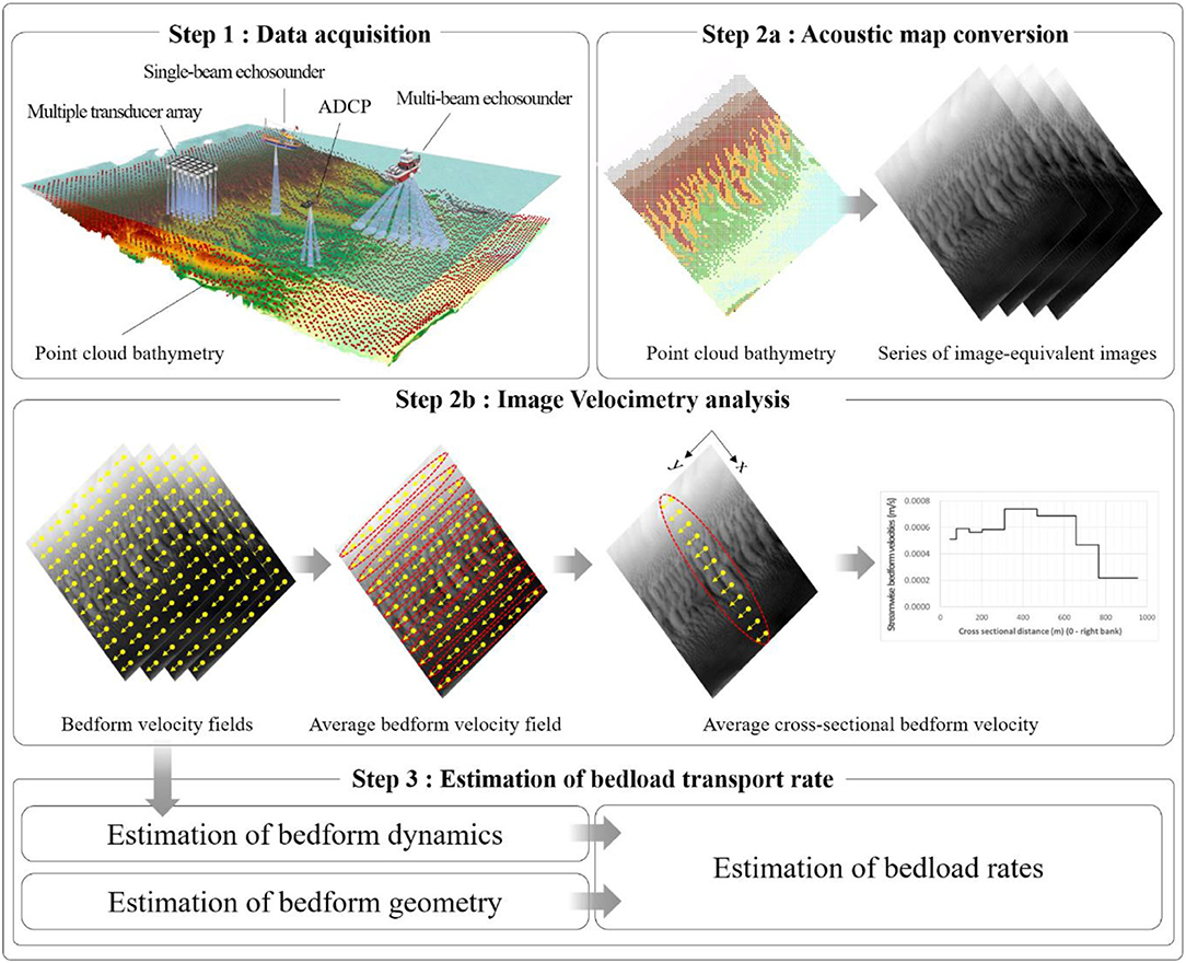
Figure 1. Description of the IV component of AMV concept.
In the first part of the second step (Step 2a), the acoustic point-cloud maps are transformed to “image-equivalent” raster files. The transformation entails a conversion of the scatter points acquired by MBES in a continuous gridded river bed surface using a linear interpolation for grid points between the MBES directly measured points (e.g., Isenburg et al., 2006; Hu et al., 2011). The new gridded surface is subsequently converted to gray-level values, as illustrated in Figure 1, Step 2a (light gray zones indicate deep bed areas, i.e., low elevations). The user determines the optimal resolution for the images by considering two desired outcomes: (i) attaining a reasonably fine resolution that accurately replicates the bed form geometry, and, (ii) limiting the output image size, as the computational demand of processing the images increases with the pixel-size of the image. The established pixel resolution (i.e., 0.5 meter per pixel) is used for all acoustic mapping conversions.
In the second part of the second step, the images obtained in Step 2a are processed using one of the IV processing techniques to obtain velocity fields that describe the 2-D bedform movement. Our research group tested three IV processing techniques to be used in conjunction with AMV: the conventional cross-correlation method (CCM), (Fujita et al., 1998); the Optical Flow Method (OFM), (Horn and Schunck, 1981); and a hybrid CCM-OFM approach called High-Gradient Image Velocimetry (HGPIV), (You et al., 2021). The CCM-based algorithms use the Fincham and Spedding (1997) approach, whereby cross-correlation is applied to gray-level patterns in the image rather than to point clusters. Given that the HGPIV method has proved superior in accuracy and computational efficiency points-of-view compared to CCM and OFM, we will use HGPIV for the present analysis. Figure 1, Step 2b illustrates the spatial and cross-section average velocity distributions obtained with HGPIV. In Step 3 of the AMV (bottom of Figure 1), the geometrical and dynamic information extracted from the acoustic maps and IV processing are combined using the Exner equation (Graf, 1984, p. 289) to estimate the bedload transport rates (Muste et al., 2008).
Implementation Considerations
Bedform geometry and dynamics are best determined from in-situ bathymetric surveys acquired in the stream wise direction to enable tracking of the bedform variation over several wavelengths. Direct measurement of the dune migration velocity (a.k.a. celerity, translational speed) are still scarce, mostly because of technological and cost limitations (Aberle et al., 2012). With the advent of acoustic instrumentation, this information is increasingly available by, for example, applying cross-correlations to a sequence of bedform linear profiles extracted from bathymetric surveys (Engel and Lau, 1981; Leary and Buscombe, 2020). These technological advancements increasingly enable researchers to monitor bedform morphology and dynamics through in-situ experiments. However, currently the rules of thumb for in-situ data acquisition are not sufficient to provide the guidance needed to ensure reliable measurements.
The final quality of the AMV results is commensurate with the adequacy of the selection of the data acquisition and processing parameters for all the processing phases shown in Figure 1. The primary requirement for quality AMV results is high resolution of the acoustic maps. The map resolution is determined by the multi-beam sounding density, which in turn depends on factors such as water depth, beam footprint area, across-track beam spacing, ping rate, and vessel speed. Duffy (2006) sets forth rigorous survey planning and protocols for ensuring high quality maps. As proven by multiple published accounts, the use of high-end spatial resolution MBES ensures that the bedform characteristics can be adequately captured down to a scale of smaller dunes or ripples moving within the largest dunes in large rivers (e.g., Cisneros et al., 2020).
The least investigated aspects of the AMV implementation are the establishment of: (a) the area of the bed to be “imaged”; (b) setting the time step between repeated acoustic map acquisitions; and, (c) selection of an adequate IV approach for acquiring the best possible result from the maps. We will provide easy-to-implement protocols for the IV-related aspects of AMV, as they directly affect both the accuracy and the cost of the measurements. Note that the goal of the measurements will dictate the selection of these factors. The requirements for measurements supporting scientific investigations (e.g., understanding of bedform mechanisms, change in the bedform structures with flow characteristics) are more stringent than those serving monitoring aspects (developing sediment ratings for bedload, sediment budget, etc.). Regardless of the measurement goal, the most reliable AMV results are obtained when the sediment transport is in equilibrium. Flows in transition require implementation of customized protocols.
The selection of the first two above-mentioned factors (directly related to the bedform shape, spacing, their spatial distribution, and the magnitude of the migration velocity) are critical as they define the size of the AMV “measurement volume” and ensure that the number of visualization patterns included within is adequate for a representative measurements. In contrast with the IV implementation to planar seeded flow, where the characteristics of the visualization patterns in IV situations are easily observed from the acquired images, knowledge of the bedform shape and distribution is not apparent and, in many situations, is totally unknown when the AMV is applied to a new site. Our subsequent discussions will focus on protocols for estimating the size of the “imaged” area and the time between successive maps in order to accurately retrieve the bedform geometry and dynamics from the acquired data. The choices used for selection of the first two factors determines the selection of the third one, i.e., the most suitable IV processing alternative. Fortunately, multiple processing approaches are available to accommodate image-equivalent acoustic maps of various quality (e.g., Cowen and Monismith, 1997; Westerweel et al., 1997; Willert, 2008).
Analytical Considerations on Bedform Geometry and Dynamics
In the absence of previous information on the bedform characteristics at a measurement site, the AMV user has no alternative in designing the measurement protocols other than relying on analytical estimates. Unfortunately, choosing analytical estimates is not without challenges as currently there is a lack of consensus on the mechanisms controlling dune geometry and dynamics, hence a lack of a solid basis for their estimation. This is reflected by the large number of relationships on bedform geometry and dynamics published in literature (Karim, 1999; Gaeuman and Jacobson, 2007; Bradley and Venditti, 2017), the contrast between laboratory and field findings (Cisneros et al., 2020), and by the fact that even the most often-used relationships are not able to predict bedload transport rates to within better than one order of magnitude (Ancey, 2020b).
The analytical and semi-empirical description of the bedform geometry and dynamics are typically offered as “scaling relationships” relating flow conditions with the sedimentary characteristics at specific sites (Bradley and Venditti, 2017). An alternative grouping of these relationships can be made based on the nature of the variables, i.e., local or global. Local methods, based on relationships between flow velocity and bed-grain size (e.g., Meyer-Peter and Müller, 1948; Van Rijn, 1993), distinguish between various bedform and flow regimes and use additional dimensionless parameters such as the Shields stress parameter, the shear Reynolds number, and the Froude number (ASCE, 2008). The local methods are rarely verified with in-situ measurements due to instrument limitations and measurement complexity. The global methods are more feasible for field studies as they define the dune geometry and dynamics with fewer hydraulic variables (e.g., Simons et al., 1965). The most widely used dune scaling relationship links bedform dimensions to flow depth (Yalin, 1964). Regardless of their type, most of these relationships assume that the bedforms are unidirectional (one-dimensional), fully developed, and in equilibrium (i.e., the geometry and dynamics remain quasi-constant with flow strength change).
For this context, we prefer using global relationships not only because they require less apriori measurements but because they entail bulk flow variables that are easier to estimate by an experienced hydrometrist. Our AMV method relies on the dune migration model originally developed by Exner (Graf, 1984, p. 289) where the entire dune cross-sectional area passes through a given point on the bed in a finite time. To the extent that the moving sediment is cycled within bedforms, the bedload transport rates can be obtained as the product of dune cross-section and the migration rate determined with dune tracking methods (Claude et al., 2012). This model entails important simplifications as the dunes can take multiple forms depending on the Froude number and bed sediment material (ASCE, 2008, p. 82), as well as on the sediment layer porosity (Simons et al., 1965). In the AMV data acquisition phase, the most important estimates are for the geometry of the largest bedforms as they dictate the size of the area to be surveyed in-situ.
The bedform (interchangeably labeled as “dune” herein) geometry and dynamics used for estimations of the much-needed bedload transport rates are typically conceptualized as sequences of triangular shapes moving in the stream wise direction. The definitions used in this paper are conform with those suggested by Gomez (1991) whereby bedload transport rates are considered local, mean values and bed-load discharge defines the cross-sectional transport rates at a specific time. The dune geometry is defined by their height, H, and length, L. The dune dynamics is related to their migration velocity, U. While H and U are typically used as average values of the respective variables, the dune height characterizing the thickness of the moving bed layer, H, is defined as half of the average dune height (e.g., Simons et al., 1965). Given that natural river beds display variable depths and a range of dune sizes across the section (i.e., approximately two orders of magnitude variation in dune height and length at any given flow depth), the above variables are most-often provided as cross-sectional distributions. Our short summary on the analytical estimation of bedform characteristics entails an often-cited reference (ASCE, 2008) and two recent compilations on bedform dynamics documented with large datasets acquired with conventional and new measurement technologies (Bradley and Venditti, 2017; Cisneros et al., 2020). Table 1 provides a summary of the parameters of interest offered by these studies.
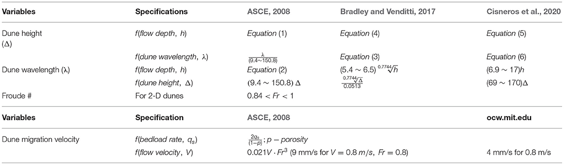
Table 1. Selected predictive formulas for estimation of bedform geometry and migration.
According to ASCE (2008), the height and wavelength of dunes migrating in equilibrium are related as follows:
And
The Bradley and Venditti (2017) analysis of relationships for estimating bedform characteristic is based on the most extensive laboratory and field dataset compiled for this purpose, according to the authors. This summary includes high spatial resolution measurements acquired with MBES surveys. The analysis is built around the often-used bedform prediction formulas that assume that the formative flow depth (h) and bedform height (Δ) are related as Δ = h/6 and length of the bedform length (λ) is related to depth as λ = 5 h. Additional clustering of these relationships is obtained by considering the median grain size of the bedform (d50) and Froude number (Fr) by Yalin (1964) and Karim (1999), respectively. Merging old and new data, Bradley and Venditti find that, for typical conditions, the bedform height and length follow a power law of the form:
and the most probable relationship between bedform height and depth is:
The Bradley and Venditti (2017) analysis concludes that there is an apparent scaling break for shallow flows, i.e., <2.5 m depth, and that use of the more complex local relationships do not substantially improve their predictive power. Bedform height in shallow flows (h <2.5 m) were found to be strongly asymmetric with high lee angles leading to bedforms larger than 6 h. The deeper channel bedforms are found to be more symmetric, with lower lee angles and relatively shorter than 6 h.
The other major contemporary compilation on dune characteristics, is the study by Cisneros et al. (2020). This compilation, complementing the previous work of Bradley and Venditti, focuses on the detailed quantification of the morphology of dunes in large rivers derived from high-resolution bathymetric datasets. The study highlights that the low-angle dunes dominate in both shallow and deep large rivers and that the lee-side shape is complex and scale dependent, while features are not considered in current dune modeling. The study finds that, for all depths, the majority of the geometrical analysis indicates:
The data analysis suggests that, for flow depths larger than 30 m, the ratio is 0.17. For 50% of the dunes the ratio values are 0.056, and for 90% of them the ratio is below 0.127. These findings substantiate that smaller dunes superimposed on the average formative dunes can be significant (>25%), contrary to the commonly made assumption that large rivers must be characterized by large dunes. The dune wavelength to dune height ratio varies widely, i.e.,
Sensitivity Analysis to Data Acquisition and Data Processing Protocols
In this section, we focus on the sensitivity of the average stream wise bedform velocity to user-determined data acquisition and processing parameters. The bedform velocity distribution is the final IV product subsequently used by AMV to estimate the bedload transport rates, as illustrated in Figure 1. The sensitivity analysis entails testing various protocols for MBES data acquisition and IV processing using an extensive dataset collected by the U.S. Army Corps of Engineers (USACE) in the Mississippi River. The dataset was used by USACE to determine rates of bedform transport with the Integrated Section Surface Difference Over Time (ISSDOT) method (Abraham et al., 2011). Given that the ISSDOT and AMV methods require similar data inputs, the available surveys can be used for conducting the preset AMV sensitivity analysis.
Benchmark for AMV Sensitivity Analysis
The dataset used for the sensitivity analysis was collected at River Mile 435 of the Mississippi River, near Vicksburg, MS, U.S.A. on April 29, 2013 (Jones et al., 2018; Ramirez et al., 2018). At the survey time, the river width was about 1,000 m, with a depth of 10 m, carrying a flow of 32,050 m3/s on a sandy bed material (d50~0.4 mm). The maximum bedform wavelength and height were 80 and 3 m, respectively. Ancillary data collected by USACE in the vicinity of the test section reach (USGS #07289000) show that the discharge varied < ±5% in the 2 days before and after the day of the MBES measurements (https://nwis.waterdata.usgs.gov/nwis). The quasi-constant discharge allows us to assume that the flow was in steady conditions at the time of the measurements, with the bedform moving in quasi-equilibrium.
The bathymetric survey was conducted over a 1,290 m wide and 990 m long area of the Mississippi River, as shown in Figure 2A. Point-clouds of various depths were acquired with a 250 kHz Geoswath 4R (geoacoustics.com) installed on a boat equipped with a Real-Time Kinetic-Geographic Positioning System (horizontal spatial accuracy of +/−2 cm, and vertical resolution of about 3 cm for 50 m flow depth). The sensor specifications are listed in Table 2. Twelve consecutively acquired stream wise swaths of about 100 m width were collected by USACE, as illustrated in Figure 2B. The cross-sectional survey required an average of 1.5 hours. Four repeated MBES surveys were continuously acquired with a spacing between repetitions of about 1.5 hours. Figure 2C shows the actual times between individual stream wise swaths for the surveys used to create the first two acoustic map pair. As can be observed from the last three columns of the table in Figure 2C, the time interval between the acquisition of individual swaths in the three image pairs (i.e., dt1, dt2, dt3) is quasi-constant foreach image used in the analysis. For such a situation there are no significant errors in determining the whole-vector velocity field using the average of all individual swath acquisition times. We actually recommend the implementation of this acquisition approach as a rule of thumb for collecting the raw MBES data. The recommended protocol is only valid under the assumption that the bedform migration is in equilibrium (i.e., the individual swaths are not experiencing variations in the mean migration rates).
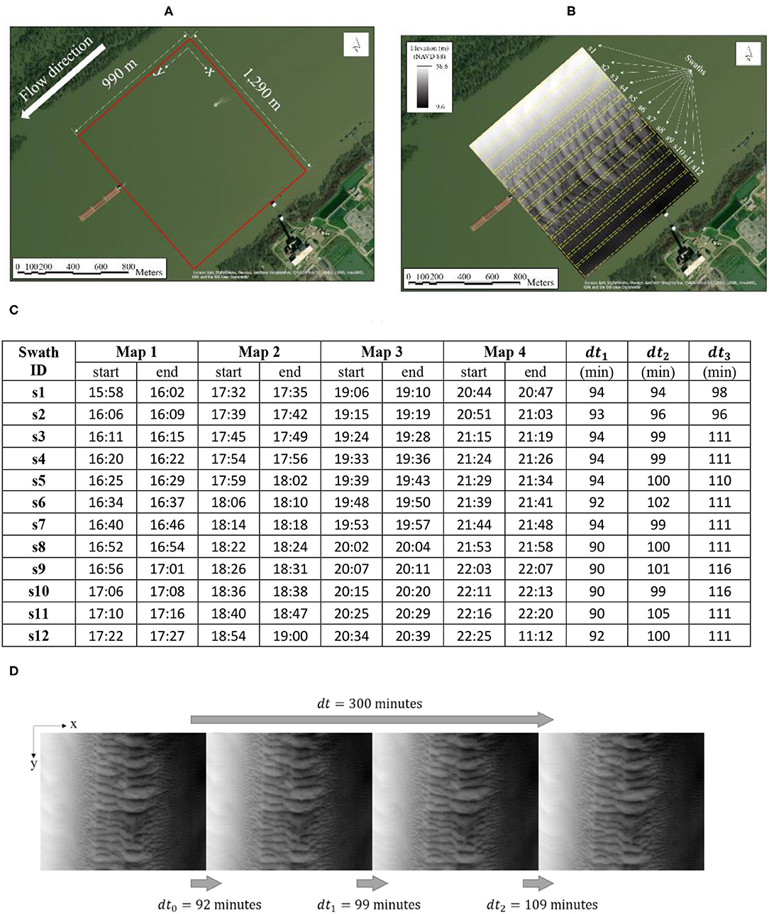
Figure 2. Sequencing of data acquisition for assembling the acoustic maps: (A) aerial photo of the study site; (B) MBES data acquisition procedure; (C) timing of the individual swaths used to construct the acoustic maps; (D) acoustic maps assembled by stitching together the stream wise MBES swaths.
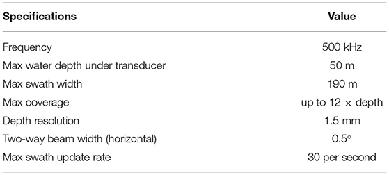
Table 2. MBES specifications.
The raw input for the AMV consists of acoustic maps obtained by stitching together the MBES stream wise swaths into one map covering the entire cross-section. These acoustic maps are ASCII files which store the horizontal location and elevation. Prior to applying IV algorithms to the acoustic maps, we converted the color-coded depth measurements into gray-colored pixels using the conventional 0–255 scale (e.g., Poynton, 1998). The conversion entails two steps (Baranya and Muste, 2016). First, the user decides on the desired resolution of the pixel image as a trade-off between attaining the desirable resolution for describing the bedform patterns of interest in the acoustic maps and limiting the output of the image size, as the computational demand of processing increases with the size of the images. In this case, we used an image size of 1,140 by 880 pixels. 1 pixel in the image corresponds to 1 m2 in the acoustic maps. Figure 2D shows the series of gray-color images derived from the four repeated surveys across the stream. Definitely, the image sampling frequency is the most important factor in correctly capturing the dynamic range of the resultant velocity field. As we stated in the paper the time ~100 minutes time separation between images was sufficient to distinguish velocities of small and large bedforms. It was not the magnitude of the bedform velocity that required special attention (as the velocities varied between 0.0002 and 0.0007 m/s) but the adjustment of the size of the interrogation area to resolve the bedform features to which the velocity is attributed to.
The twelve MBES stream wise swaths assembled for the creation of the maps reveal large variations in the bedform geometry across the section. Based on the bedform geometry analysis guided by visual inspection of the maps, we identified eight distinct bedform regions, as illustrated in Figure 3A. The large variety of bedform sizes are a direct result of the high-gradients in the depths and velocities across the section, as illustrated by the ADCP measurements in Figure 3B. Using the MBES data as raw input, we estimated the bedform geometry with three alternative methods, as shown in Table 3. Column three of the table contains the outcomes of applying the Bedform Tracking Tool (BTT) developed by Van der Mark et al. (2008) to the MBES survey. In general, the results in Table 3 are in good agreement with the dune population statistics produced by the analysis of linear profiles of the bedforms extracted from the bathymetric swath determined by Ramirez et al. (2018).
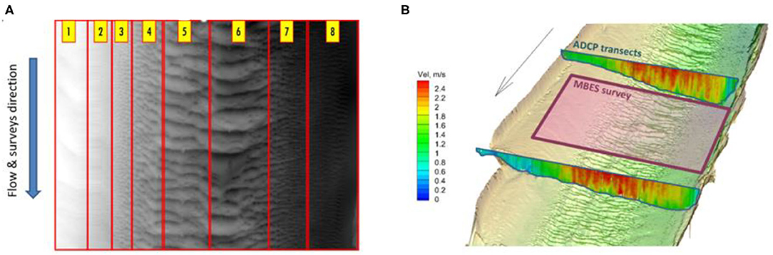
Figure 3. Zoning of the MBES map with considerations of the cross-sectional distribution of the bedform characteristics: (A) bedform elevations; (B) velocity and depth distributions.
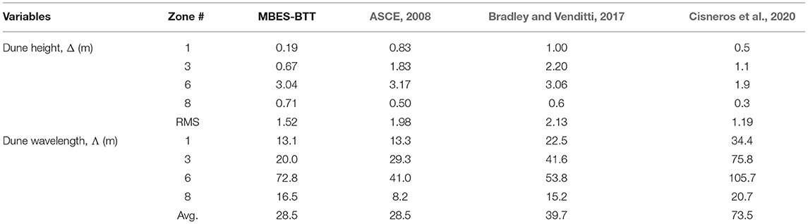
Table 3. A comparison of analytical estimates for the Mississippi dataset (see Figure 2) with the results of MBES-BTT statistical package analysis.
Sensitivity to Data Acquisition Procedures
Acoustic Map Quality vs. MBES Swath Overlapping
Due to the limited span of the MBES measurement footprint, most of the acoustic maps for typical rivers require the acquisition of multiple swaths to cover the entire river width. Typically, the swaths are collected along survey lines aligned with the stream wise direction. However, if the MBES footprint contains several large dunes within, the survey can also be acquired along transects across the river. Regardless of the navigation mode, attention has to be given to the overlaps between adjacent survey lines. Duffy (2006) proposed an overlay of up to 50% of adjacent survey lines as optimal for a better description of the bedform geometry. In the same study, however, “free-hand” survey lines were also acquired whereby the lines barely touched the outermost beams of the previous lines. There was not a drastic difference in the quality of the maps. The experienced team of USACE surveyors do not overlap the swaths more than 15% and the quality of the obtained maps has been satisfactory. Given these experiences, we have deemed that the density of the cloud-points from one passing of the MBES is sufficient for accurately replicating the bed topography.
Bedform Geometry Estimation vs. Streamwise Length of the Acoustic Maps
This analysis uses as reference the bedform geometry determined using the full size of the acoustic maps (1,290 m wide and 990 m long area) and all four maps collected in the benchmark set. Figure 4 compares the BTT-estimated bedform heights for the eight dune regions using 75, 50, and 25% of the longitudinal MBES survey lines and all four repeated acoustic maps (see Figure 2D). As expected, the plots show that a reduction of up to 50% of the longitudinal length of the acoustic map does not have a considerable effect on the reconstruction of the smaller geometry dune characteristics. However, a reduction of more than 50% of the longitudinal length produces a 14% difference in the estimation of the average dune height for the zone containing the largest dune wavelengths. Taking into account the number of dunes in the area with the largest bedforms, we conclude that considering 5–6 dunes suffices for determining their geometry. Note that a heuristic estimation proposed by Le Guern et al. (2021) recommends surveying 10 dunes for capturing their representative profiles. From this point, we will continuously relate the sensitivity analysis to large dunes, which for the present context is justifiable as the largest bedforms are the dominant contributors to the bedload estimation, and the ultimate result targeted by AMV technique.
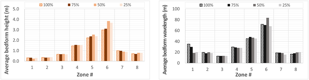
Figure 4. Sensitivity of the bedform characteristics to the longitudinal dimension of the acoustic map: (A) average bedform height; (B) average bedform wavelength.
Bedform Geometry Estimation vs. the Number of Repeated Acoustic Maps
The practice of acquiring repeated images for IV processing and averaging them over time stems from traditional PIV where the repeated measurements are necessary because the density of the seeding (e.g., visualization particles) in the area to be measured is often non-homogeneous and changes quickly in time and space. Even if the rules of thumb to assure uniform and homogeneous seeding are fully implemented, acquiring multiple images taken in short bursts remains the standard practice in conventional PIV. In contrast with conventional PIV, visualization of the bedforms with acoustic instruments is greatly facilitated by the fact that the dunes are in actuality continuous and compact layers migrating very slowly. In spite of these advantages, challenges still exist in obtaining accurate acoustic maps.
Most of the challenges are related to the instrument configuration (e.g., the sounding density and spatial resolution is strongly nadir biased), navigation issues (e.g., heave-related bias), and changes in the water column density due to fluid stratification for some situations (Duffy, 2006). Consequently, there is no question that the more repeated measurements are taken the better the resolution of the obtained maps. The previous experience shows that with proper caution and, if needed, corrections, a single MBES-acquired acoustic map provides adequate information for a qualified acoustic map. Moreover, repetition in itself does not necessarily improve the acoustic map accuracy as the swath acquisition takes a finite amount of time while the dunes continue to migrate. Consequently, the images taken from repeated swaths are close to each other but not identical. Thus, their averaging can actually be detrimental. Last but not least important, is that increasing the number of maps increases sensibly the measurement cost, therefore cost-benefit analysis need to be considered.
Our perception is that one pair of well-acquired acoustic maps suffices for characterization of the bedform geometry. This is supported by the illustration in Figure 5 where the bedform characteristics are determined with MBES measurements obtained as averages over 1, 2, and 3 acoustic maps are compared with the same information obtained from all available images for the benchmark dataset. We obtained the plots in Figure 5 with the full length of the longitudinal dimension of the available acoustic maps. The plots do not display differences larger than 10% for the bedform heights and wavelengths estimated with BTT in any of the eight zones of the acoustic maps.
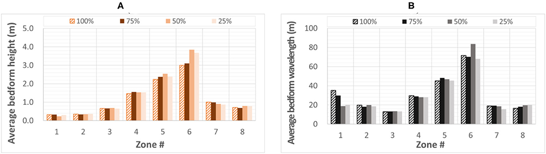
Figure 5. Sensitivity of the bedform characteristics to the number of images used to extract the information: (A) average bedform height; (B) average bedform wavelength.
Given that the bedform geometry estimation is also dependent on the length of the survey lines, we plot in Figure 6 various scenarios whereby we progressively change both the length of the longitudinal dimension of the acoustic maps and the number of acoustic maps used for averaging the bedform geometry. The visual inspection of the plots reinforces the conclusion that half of the length of the originally surveyed area (corresponding to about six bedform wavelengths) and one pair of acoustic maps provide reliable acoustic maps in comparison with the reference. Any decision regarding suitable combinations of operating protocols should start with a stream wise map length of 5–6 wavelengths and one pair of repeated maps as a minimum scenario (see Figure 5). Final decisions should be based on a cost-benefit analysis, with consideration of the scope of the measurements.
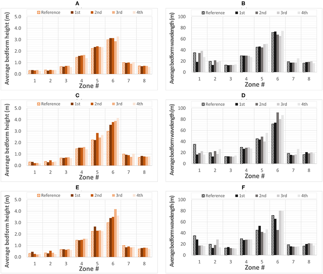
Figure 6. Sensitivity of the bedform characteristics to the combined effect of a number of processed acoustic maps and length of the survey line: (A,B) average bedform height and wavelength for 1, 2, and 3 processed acoustic maps and 75% of the full length of the benchmark surveyed area, respectively; (C,D) average bedform height and wavelength for 1, 2, and 3 processed acoustic maps and 50% of the full length of the benchmark surveyed area, respectively; (E,F) average bedform height and wavelength for 1, 2, and 3 processed acoustic maps and 25% of the full length of the benchmark surveyed area, respectively.
Acoustic Map Relevance vs. Number and Timing of the Individual Swaths
The number of longitudinal swaths depends on the river width and depth range in the targeted measurement section, and the footprint of the MBES (variable with the depth). The timing between consecutive swaths depends on the time it takes to cover the minimum of 5–6 wavelengths for the largest bedforms in the cross-section. The total time for obtaining one acoustic map is then determined by the sum of the time it takes to acquire all longitudinal swaths and the time to move the sensor array from one swath to the next. For the benchmark dataset used herein, we obtained one map in about 1.5 hours (see Figure 2).
It is obvious from the above considerations that the resultant cross-section map will contain multiple bedform profiles taken at slightly different times. Similar to other scanning measurements (e.g., atmospheric boundary layer lidars), the relatively short time for surveying the river bed compared to the slow progression of the bedforms can be considered “instantaneous” for mapping purposes. This assumption is acceptable only if the sediment transport at the time of mapping is in equilibrium regime. Given the above constraints, the MBES operator had to make tradeoffs between reducing the length of the longitudinal survey lines and increasing the navigation speed in a manner that shortens the acquisition time as much as possible to get closer to a “snapshot” situation.
Bedform Dynamics vs. Acoustic Map Sampling Frequency
The minimum time for repeating the maps cannot be shorter than the total time for acquiring the bedform map over the whole targeted area. The maximum allowable time is dependent on the bedload migration velocity, perhaps the variable most difficult to predict for a specific site and flow condition. Ideally, the acoustic map survey frequency should be high enough so that the largest dunes do not migrate more than half of their wavelength between maps (Duffy, 2006). Here again, the sensitivity is referenced to the geometry of the largest dunes that might result in obscuring the accurate estimation of the smaller bedform dynamics.
In addition, the IV processing requirements specify that the displacement of the image patterns used for determining the velocities should be smaller than one quarter of the pattern displacement between the two images in the pair but larger than 2 pixels (Willert and Gharib, 1991). Consequently, we recommend selecting a sampling frequency within the limits of the two set of constraints. For the benchmark dataset used here as reference, the largest wavelengths are 80 m with a migration velocity 0.0007 m/s. The resultant maximum time between acoustic maps is 1 day and 8 hours, and the minimum time is 2.5 hours. The 1.5 hours used for of the acquisition of the map is close to fulfilling both requested criteria, with potential losses in accuracy regarding the velocity estimation for the smallest bedforms in the maps.
While extraction of longitudinal profiles from of an acoustic map over bedform in equilibrium regime can be considered reliable, the reconstruction of the bedform dynamics is unquestionably more problematic when obtained with time delays between individual MBES swaths. Especially problematic are situations where the bedform dynamics are driven by prominent 2-D planar movement. If the dunes are migrating only along the stream wise direction, each longitudinal swath cuts across the bedforms at slightly different times (as shown in Figure 2). When the derived maps are superimposed, discontinuities are produced at the swaths' junctions, in the area of swath overlapping. This deformation of the patterns does not pose considerable issues for the IV processing as the vector estimation is made with parameters that are much smaller in size than the swath widths. To minimize the effect of time differences between individual swaths, we recommend acquiring the maps with identical surveying protocols both in space and time. In other words, the repeated maps should follow identical sequencing for the acquisition of the stream wise swaths with care to maintain the duration of each individual swath as constant as possible.
Bedform Dynamics vs. the Size of the Acoustic Map
The number of image pairs, and their timing. The dynamic qualifier for the bedload in the present context is the bedform's averaged velocity profile across the river width. This velocity distribution serves as an input in the estimation of the bedload transport rates with AMV (as shown in Figure 1). This profile is obtained as the average if the global vector field projected on a central cross section. Similar to the estimation of the bedform geometry, the estimation of the bedform dynamics over the cross-section is dependent on the longitudinal size of the acoustic map and the number of acoustic map pairs used for determining the velocity fields.
The plots in Figure 7 feature the cross-sectional distribution of the average bedform velocity. These plots reflect the impact of the stream wise length of the surveyed area and the number of repeated maps on the bedform's averaged velocity profiles. Similar to the sensitivity analysis of the bedform geometry, we observed a deterioration of the quality of the velocity profile for reduced stream wise length of the maps, irrespective of the number of images used for processing. A related sensitivity aspect is shown in Figure 7E to demonstrate that the shorter the time interval between the image pairs, the better the agreement with the benchmark reference.
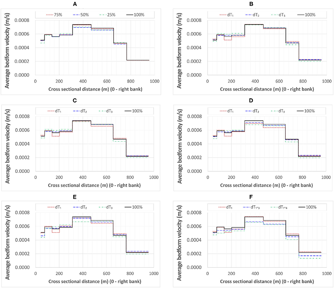
Figure 7. Sensitivity of the bedform dynamics to the number of processed acoustic maps and length of the survey line (plotted as cross-sectional distributions): (A) average velocity field estimated with all acoustic maps and 100% (reference), 75, 50 and 25% of the full size acoustic image; (B) average bedform velocity field estimated from all the acoustic map pairs over full size of the maps (reference) compared with the same as obtained from image pair 1 and 2, pair 2 and 3, and pair 3 and 4; (C) average bedform velocity field estimated with all acoustic maps and full size map (reference), compared with 75% of the full size acoustic image; (D) average velocity field estimated with all acoustic maps and full size map (reference), compared with 50% of the full size acoustic image; (E) average bedform velocity field estimated with all acoustic maps and full size map (reference), compared with 25% of the full size acoustic image; (F) average velocity field estimated with all acoustic maps and full size map (reference), compared with the same obtained from pair 1 and 2, pair 1 and 3, and pair 1 and 4.
Sensitivity to IV Approach and Processing Parameters
Choice of IV Processing Approach vs. Accurate Replication of the Bedform Dynamics
For the context of dune tracking, an image velocimetry technique closer to Particle Tracking Velocimetry (e.g., Dracos, 1996) would seem more natural as the goal of the IV is to track linear features moving in quasi unidirectional direction. Duffy's (2006) IV approach follows this avenue. However, given our extensive experience with Large-Scale Particle Image Velocimetry, we approach this new area of application using PIV approaches customized for dune tracking. Moreover, we rarely mention the PIV term in isolation as, especially for this application case, the particle images per se are actually quite irrelevant, which is in contrast with the seeding particles used in the conventional PIV. Instead, we use more often the term Image Velocimetry (IV) as we deem to be more appropriate for the context. We consider that IV as presented in this paper can add value in comparison to PTV implementation for documenting the migration of two-or three-dimensional bedforms or to track the movement of the ripples traveling atop of the large bedforms. In this cases the bedforms can deform and maybe more difficult to be tracked by PTV algorithm.
In the initial stage of the AMV development, we used the CCM approach (Raffel et al., 2007). Key elements for ensuring CCM processing accuracy include the adequate selection of the size of the elemental area containing the patterns to be tracked, and the size and orientation of the Search Window (SW) where the pattern displacement is determined (Adrian, 1991). Regardless of the choice made in selection, use of the same set of parameters for processing the whole imaged area with the CCM does not accurately resolve the movement of patterns if they are significantly different in size and velocities. Such large differences are common for the images processed by AMV, as the bedform characteristics vary widely across the stream cross-sections. Because of this, more flexible algorithms that adapt the processing parameters to the local image pattern characteristics should be used, ideally in an automated mode.
We tested the possibility for overcoming these CCM limitations using: (i) a new approach to the Optical Flow Method (OFM) that combines elements from Horn and Schunck (1981); Lucas and Kanade (1981) and, (ii) a new CCM-OFM hybrid approach we developed called HGPIV (You et al., 2021). The improvement is brought about the first approach is that OFM are superior to CCM in terms of spatial resolution and smoothness of the vector field. The second approach combines the benefits of CCM and OFM and considerably reduced the computational time. The HGPIV determine first the optimal SW for CCM processing using OFM protocols. The optimal SW detection is iteratively executed for the whole image area without user intervention. The comparison of the accuracy and computational efficiency of the three IV processing approaches led to the conclusion that the HGPIV hybrid is the best candidate for extracting velocity-vector fields with high-gradient velocities (You et al., 2021).
Figures 8A–C show vector fields obtained with above mentioned algorithms applied to the four repeated maps acquired over the full size area of the benchmark data acquired in the Mississippi River using. Figure 8D compares the averaged bed form velocity distribution for the eight zones delineated in Figure 3A. A more detailed view of the bed form dynamics is further illustrated by considering a 1.5 size bed form wavelength in Zone six of the benchmark dataset in Figure 8E. The velocity distributions over the specified bed form area display a realistic variation of the velocity distribution within a dune in Figures 8F–H. The latter plots illustrate the power of the AMV for exploration of the bed form migration at scales that are relevant for understanding fundamental aspects of the bed form transport process.
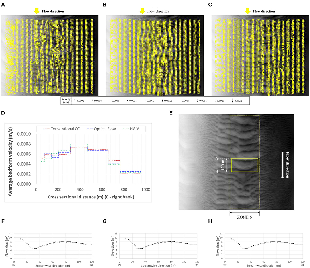
Figure 8. Comparison of various IV approaches used in conjunction with AMV: (A–C) bedform velocity spatial distribution over the surveyed area obtained with CCM, OFM, and HGPIV, respectively; (D) comparison of the cross sectional average bedform velocities obtained with the three IV approaches; (E) area of detailed observation within the acoustic map; (F–H) distribution of the averaged velocity at the surface of the bedform enclosed in the area shown in this figure (E).
Choice of Interrogation Area (IA) Selection vs. IV Dynamic Spatial Range
Application of CCM and OFM to planar flow images of quasi-uniform velocity distributions is relatively mature with rules of thumb for guiding the user assembled in multiple published accounts (e.g., Adrian, 1991; Scharnowski and Kähler, 2020 for CCM; Tauro et al., 2018 for OFM). The guidance for ensuring spatial resolution and dynamic spatial range entails rules that connect the image resolution with the parameters used in processing. The newer HGPIV approach does not benefit from similar guidance. However, given that HGPIV is a hybrid between CCM and OFM, all the relevant rules pertaining to the latter two techniques apply.
The key parameter for the IV processing approaches tested herein is the selection of the size of the IA. Regardless of the IV approach, the user establishes the IA based on the inspection of the geometry and dynamics of the patterns used for visualization, and the resolution of the grid for reporting the IV processing outcomes. Specifically, the IA should be large enough to encompass within it easily recognizable or unique image patterns. If the IA is too small, no vectors, or spurious ones, might result as the small changes within the feature pattern might confuse the pattern matching between the image pairs. If the IA is too large, the software is probably tracking the most prominent features that usually pertain to larger size patterns washing out the information associated with the movement of the smaller bedform features (e.g., ripples migrating between dunes). In essence, the establishment of the IA is a result of a preliminary trial-and-error analysis conducted for all sub-areas of the acoustic image. The quality of the analysis outcome depends on the user's familiarity with aspects of image acquisition and processing, in addition to a good understanding of the flow features to be documented.
Summary and Conclusions
Our recent approach to IV implementation for estimating bedform geometry and dynamics with AMV carries new challenges due to both the nature of the images to be analyzed and their spatio-temporal characteristics. In contrast with the conventional IV approaches, where the operator can visualize the flow appearance prior to the acquisition and processing of the data, the AMV measurements are taken in much more uncertain conditions, with flow features that cannot be anticipated without prior measurements at the site or analytical estimations of the features to be measured. Unfortunately, prior information is, in most cases, lacking, and analytical estimates for bedform characterization are notoriously imprecise and vary widely with the flow regimes and bedload material. Given this situation, new measurements with AMV are intrinsically heuristic, requiring an understanding of the flow and the means to experimentally document flow features. Table 4 provides general recommendations regarding the best approaches for making these measurements.
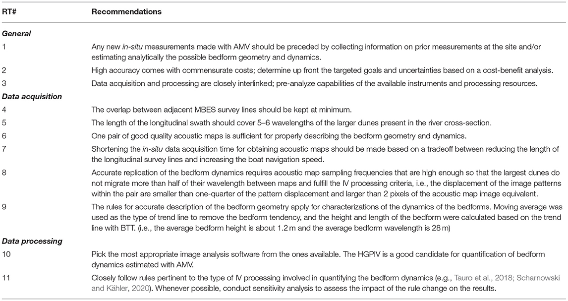
Table 4. Rules of thumb for in-situ implementation of IV component of AMV.
Given that AMV is in the early stages of development, there are multiple possibilities for optimization and improvement of the technique's accuracy. We consider it useful and timely to share our experiences with respect to the practical rules that maintain the measurement outcome accuracy with reduced costs, and without adding complexity to an already complex task. The major contribution of these rules is that they provide the user with practical, easy to understand procedures related to in-situ data collection protocols and image processing. Especially relevant for reducing the time and expense associated with data collection is to decide on the optimum combination between: (i) the targeted resolution for the acoustic mapping; (ii) the size of the survey area, and, (iii) the timing between the successive acquisition of the acoustic maps. Table 4 summarizes the rules for data acquisition and processing described in Section Sensitivity Analysis to Data Acquisition and Data Processing Protocols. Practical rules for the selection of image processing software and optimization of the some of the ancillary parameters are provided in the same table.
We have successfully used AMV for characterization of the bedform geometry and dynamics in several prior studies conducted. This paper is an additional and eloquent demonstration of the power, simplicity, and cost-effectiveness of the quantification of the bedform dynamics with such non-intrusive in-situ measurements. It also underscores that, despite its ease of use and efficiency, the implementation of the technique requires expert knowledge on flow, the measurement techniques, and the adoption of rigorous protocols for data acquisition and image processing. If the user is only interested in the time-averaged qualitative overview of the bedform dynamics, the requirements regarding velocimetry are less stringent compared to the acquisition of greater detail required by the investigation for shedding light on the mechanics of river morphology. Regardless of the goal of the measurements, however, comparisons with alternative measurement methods remain the gold standard, as there is no widely recognized method for quantification of the bedform geometry and dynamics.
Data Availability Statement
The original contributions presented in the paper are based on supported data that can be inquired directly by contacting the corresponding author.
Author Contributions
All authors developed the paper concept and the plan for sensitivity analysis. HY carried out the processing for sensitivity analysis and prepared the graphically demonstrations. Review and comments on analysis were contributed by DK and SB. MM edited and prepared the final form of manuscript. All authors contributed to the article and approved the submitted version.
Funding
This work was supported by the US Geological Survey Cooperative Grant Agreement #G19AC00257 and by the Korea Agency for Infrastructure Technology Advancement (KAIA) grant funded by the Ministry of Land, Infrastructure and Transport (21DPIW-C153746-03). HY was partially supported for this effort by the NSF award EAR 1948944.
Conflict of Interest
The authors declare that the research was conducted in the absence of any commercial or financial relationships that could be construed as a potential conflict of interest.
Publisher's Note
All claims expressed in this article are solely those of the authors and do not necessarily represent those of their affiliated organizations, or those of the publisher, the editors and the reviewers. Any product that may be evaluated in this article, or claim that may be made by its manufacturer, is not guaranteed or endorsed by the publisher.
References
Aberle, J., Nikora, V., Coleman, S. E., and Nikora, V. I. (2012). Article in acta geophysica. Acta Geophys. 60, 1720–1743. doi: 10.2478/s11600-012-0076-y
Abraham, D., and Kuhnle, R. (2006). “Using high resolution bathymetric data for measuring bed-load transport,” in Proceedings of the Federal Interagency Sedimentation Conferences, 1947 to 2006 (Reno), 619–626.
Abraham, D., Kuhnle, R. A., and Odgaard, A. J. (2011). Validation of bed-load transport measurements with time-sequenced bathymetric data. J. Hydraul. Eng. 137, 723–728. doi: 10.1061/(ASCE)HY.1943-7900.0000357
Adrian, R. J. (1991). Particle-imaging techniques for experimental fluid mechanics. Annu. Rev. Fluid Mech. 23, 261–304. doi: 10.1146/annurev.fl.23.010191.001401
Ancey, C. (2020a). Bedload transport: a walk between randomness and determinism. Part 1. The state of the art. J. Hydraul. Res. 58, 1–17. doi: 10.1080/00221686.2019.1702594
Ancey, C. (2020b). Bedload transport: a walk between randomness and determinism. Part 2. Challenges and prospects. J. Hydraul. Res. 58, 18–33. doi: 10.1080/00221686.2019.1702595
ASCE (2008). Sedimentation Engineering : Processes, Management, Modeling, and Practice, ed M. Garcia (Reston, VA: American Society of Civil Engineers).
Baranya, S., and Muste, M. (2016). Validation and application of acoustic mapping velocimetry. Geophys. Res. Abstr. 18, 2016–17158. Available online at: https://ui.adsabs.harvard.edu/abs/2016EGUGA.1817158B
Bradley, R. W., and Venditti, J. G. (2017). Reevaluating dune scaling relations. Earth Sci. Rev. 165, 356–376. doi: 10.1016/j.earscirev.2016.11.004
Cisneros, J., Best, J., van Dijk, T., Almeida, R. P., de Amsler, M., Boldt, J., et al. (2020). Dunes in the world's big rivers are characterized by low-angle lee-side slopes and a complex shape. Nat. Geosci. 13, 156–162. doi: 10.1038/s41561-019-0511-7
Claude, N., Rodrigues, S., Bustillo, V., Bréhéret, J. G., Macaire, J. J., and Jugé, P. (2012). Estimating bedload transport in a large sand-gravel bed river from direct sampling, dune tracking and empirical formulas. Geomorphology 179, 40–57. doi: 10.1016/j.geomorph.2012.07.030
Conevski, S., Guerrero, M., Winterscheid, A., Rennie, C. D., and Ruther, N. (2020). Acoustic sampling effects on bedload quantification using acoustic Doppler current profilers. J. Hydraul. Res. 58, 982–1000. doi: 10.1080/00221686.2019.1703047
Cowen, E. A., and Monismith, S. G. (1997). A hybrid digital particle tracking velocimetry technique. Exp. Fluids 22, 199–211. doi: 10.1007/s003480050038
Detert, M. (2021). How to avoid and correct biased riverine surface image velocimetry. Water Resour. Res. 57, e2020WR027833. doi: 10.1029/2020WR027833
Dinehart, R. L. (2002). Bedform movement recorded by sequential single-beam surveys in tidal rivers. J. Hydrol. 258, 25–39. doi: 10.1016/S0022-1694(01)00558-3
Dracos, T. (1996). Particle Tracking Velocimetry (PTV). Dordrecht: Springer. doi: 10.1007/978-94-015-8727-3_7
Dramais, G., Le Coz, J., Camenen, B., and Hauet, A. (2011). Advantages of a mobile LSPIV method for measuring flood discharges and improving stage-discharge curves. J. Hydro. Environ. Res. 5, 301–312. doi: 10.1016/j.jher.2010.12.005
Duffy, G. P. (2006). Bedform migration and associated sand transport on a banner bank: application of repetitive multibeam surveying and tidal current measurement to the estimation of sediment transport (Ph.D. thesis). The University of New Brunswick, Fredericton, Canada.
Engel, P., and Lau, Y. L. (1981). Bed load discharge coefficient. J. Hydraul. Div. ASCE 107, 1445–1454. doi: 10.1061/JYCEAJ.0005762
Fincham, A. M., and Spedding, G. R. (1997). Low cost, high resolution DPIV for measurement of turbulent fluid flow. Exp. Fluids 23, 449–462. doi: 10.1007/s003480050135
Fujita, I., Muste, M., and Kruger, A. (1998). Large-scale particle image velocimetry for flow analysis in hydraulic engineering applications. J. Hydraul. Res. 36, 397–414. doi: 10.1080/00221689809498626
Gaeuman, D., and Jacobson, R. B. (2006). Acoustic bed velocity and bed load dynamics in a large sand bed river. J. Geophys. Res. Earth Surf. 111:2005. doi: 10.1029/2005JF000411
Gaeuman, D., and Jacobson, R. B. (2007). Field assessment of alternative bed-load transport estimators. J. Hydraul. Eng. 133, 1319–1328. doi: 10.1061/(ASCE)0733-9429(2007)133:12(1319)
Graf, W. H. (1984). Hydraulics of Sediment Transport. Highlands Ranch, CO: Water Resources Publications.
Gray, J., Laronne, J., and Marr, J. (2010). Bedload-Surrogate Monitoring Technologies, Scientific Investigations Report 2010–5091, 37. U.S. Geological Survey. doi: 10.3133/sir20105091
Holmes, R. H. (2010). Measurement of Bedload Transport in Sand-Bed Rivers: A Look at Two Indirect Sampling Methods, Scientific Investigations Report 2010–5091. U.S. Geological Survey.
Horn, B. K. P., and Schunck, B. G. (1981). Determining optical flow. Artif. Intell. 17, 185–203. doi: 10.1016/0004-3702(81)90024-2
Hu, H., Yang, Y., Jiang, Z., and Han, P. (2011). An analysis research about accuracy and efficiency of grid DEM interpolation. Commun. Comput. Inf. Sci. 144, 25–30. doi: 10.1007/978-3-642-20370-1_5
Hubbell, D. W. (1964). Apparatus and Techniques for Measuring Bedload. U.S. Geological Survey Water-Supply Paper 1748, 74. Available online at: https://pubs.er.usgs.gov/publication/wsp1748 (accessed May 25, 2021).
Isenburg, M., Liu, Y., Shewchuk, J., Snoeyink, J., and Thirion, T. (2006). Generating raster DEM from mass points via TIN streaming. Lect. Notes Comput. Sci. 4197, 186–198. doi: 10.1007/11863939_13
Jones, K. E., Abraham, D. D., and McAlpin, T. O. (2018). Bed-Load and Water Surface Measurements during the 2011 Mississippi River Flood at Vicksburg, Mississippi, MRG&P Report 18. U.S. Army Engineer Research and Development Center. doi: 10.21079/11681/27112
Karim, F. (1999). Bed-form geometry in sand-bed flows. J. Hydraul. Eng. 125, 1253–1261. doi: 10.1061/(ASCE)0733-9429(1999)125:12(1253)
Kim, Y., Muste, M., Hauet, A., Bradley, A., Weber, L., and Koh, D. (2007). “Uncertainty analysis for Lspiv in-situ velocity measurements,” in Proceedings of the Congress International Association for Hydraulic Research (Venice), 81.
Knaapen, M. A. F. (2004). “Measuring sand wave migration in the field. Comparison of different data sources and an error analysis,” in Marine Sandwave and River Dune Dynamics, eds S. J. M. H. Hulscher, T. Garlan, and D. Idier (Enschede: University of Twente), 152–160.
Le Guern, J., Rodrigues, S., Geay, T., Zanker, S, Hauet, A., Tassi, P., et al. (2021). Relevance of acoustic methods to quantify bedload transport and bedform dynamics in a large sandy-gravel-bed river. Earth Surf. Dyn. Discuss. 9, 423–444. doi: 10.5194/esurf-9-423-2021
Leary, K. C. P., and Buscombe, D. (2020). Estimating sand bed load in rivers by tracking dunes: a comparison of methods based on bed elevation time series. Earth Surf. Dyn. 8, 161–172. doi: 10.5194/esurf-8-161-2020
Leese, J. A., Novak, C. S., and Clark, B. B. (1971). Automated technique for obtaining cloud motion from geosynchronous satellite data using cross correlation. J. Appl. Meteorol. 10, 118–132. doi: 10.1175/1520-0450(1971)010<0118:AATFOC>2.0.CO;2
Lucas, B. D., and Kanade, T. (1981). Iterative image registration technique with an application to stereo vision. ACM 2, 674–679.
Meyer-Peter, E., and Müller, R. (1948). “Formulas for bed-load transport,” in Proceedings of the 2nd Meeting International Association of Hydraulic Research (Stockholm), 39–64.
Muste, M., Abraham, D., Jones, K., Wagner, D., and Whaling, A. (2019). In-situ Bedload Measurements Using Multi-beam Echosounders and Acoustic Current Doppler Profilers. U.S. Geological Survey Cooperative Agreement #G19AC00257. USGS NAtional Grants Branch.
Muste, M., Baranya, S., Tsubaki, R., Kim, D., Ho, H., Tsai, H., et al. (2016). Acoustic mapping velocimetry. Water Resour. Res. 52, 4132–4150. doi: 10.1002/2015WR018354
Muste, M., Fujita, I., and Hauet, A. (2008). Large-scale particle image velocimetry for measurements in riverine environments. Water Resour. Res. 44, W00D19. doi: 10.1029/2008WR006950
Poynton, C. A. (1998). “Rehabilitation of gamma,” in Human Vision and Electronic Imaging III, eds B. E. Rogowitz and T. N. Pappas (Bellingham, WA: SPIE), 232–49. doi: 10.1117/12.320126
Raffel, M., Willert, C. E., Wereley, S. T., and Kompenhans, J. (2007). Particle Image Velocimetry A Practical Guide, 2nd Edn. Berlin: Springer-Verlag. doi: 10.1007/978-3-540-72308-0
Ramirez, M., Smith, S., Lewis, J., and Pratt, T. (2018). Mississippi River Bedform Roughness and Streamflow Conditions near Vicksburg, Mississippi. Mississippi River Geomorphology and Potamology Program Report No. 22, U.S. Army Corps of Enginners. Available online at: https://apps.dtic.mil/sti/citations/AD1082136 (accessed April 14, 2021).
Rennie, C. D., and Millar, R. G. (2004). Measurement of the spatial distribution of fluvial bedload transport velocity in both sand and gravel. Earth Surf. Process. Landf. 29, 1173–1193. doi: 10.1002/esp.1074
Savic, D. (2019). Artificial Intelligence: How Can Water Planning and Management Benefit From It?[White paper]. IAHR. Available online at: https://www.iahr.org/library/infor?pid=8426
Scharnowski, S., and Kähler, C. J. (2020). Particle image velocimetry–classical operating rules from today's perspective. Opt. Lasers Eng. 135:106185. doi: 10.1016/j.optlaseng.2020.106185
Simons, D. B., Richardson, E. V., and Nordin, C. F. (1965). Bedload Equation for Ripples and Dunes, Professional Paper 462-H. U.S. Geological Survey. doi: 10.3133/pp462H
Tauro, F., Piscopia, R., and Grimaldi, S. (2017). Streamflow observations from cameras: large-scale particle image velocimetry or particle tracking velocimetry? Water Resour. Res. 53, 10374–10394. doi: 10.1002/2017WR020848
Tauro, F., Tosi, F., Mattoccia, S., Toth, E., Piscopia, R., and Grimaldi, S. (2018). Optical tracking velocimetry (OTV): leveraging optical flow and trajectory-based filtering for surface streamflow observations. Remote Sens. 10:2010. doi: 10.3390/rs10122010
Van der Mark, C. F., Blom, A., and Hulscher, S. M. J. H. (2008). Quantification of variability in bedform geometry. J. Geophys. Res. Earth Surf. 113, F03020. doi: 10.1029/2007JF000940
Van Rijn, L. (1993). Principles of Sediment Transport in Rivers, Estuaries and Coastal Seas. Amsterdam: Aqua Publications.
Westerweel, J. (1993). Digital Particle Image Velocimetry: Theory and Application. Delft: Delft University Press.
Westerweel, J., Dabiri, D., and Gharib, M. (1997). The effect of a discrete window offset on the accuracy of cross-correlation analysis of digital PIV recordings. Exp. Fluids 23, 20–28. doi: 10.1007/s003480050082
Willert, C. (2008). “Adaptive PIV processing based on ensemble correlation,” in 14th International Symposium on Applications of Laser Techniques to Fluid Mechanics Lisbon (Portugal). Available online at: https://elib.dlr.de/55162/ (accessed July 10, 2008).
Willert, C. E., and Gharib, M. (1991). “Digital particle image velocimetry,” in Experiments in Fluids 10, 181–193. doi: 10.1007/BF00190388
Yalin, M. S. (1964). Geometrical properties of sand wave. J. Hydraul. Div. 90, 105–119. doi: 10.1061/JYCEAJ.0001097
Keywords: bedform geometry, bedform dynamics, acoustic mapping, image velocimetry, acoustic mapping velocimetry
Citation: You H, Muste M, Kim D and Baranya S (2021) Considerations on Acoustic Mapping Velocimetry (AMV) Application for in-situ Measurement of Bedform Dynamics. Front. Water 3:715308. doi: 10.3389/frwa.2021.715308
Received: 02 June 2021; Accepted: 30 September 2021;
Published: 04 November 2021.
Edited by:
Matthew Perks, Newcastle University, United KingdomReviewed by:
Slaven Conevski, Norwegian University of Science and Technology, NorwayMassimo Guerrero, University of Bologna, Italy
Copyright © 2021 You, Muste, Kim and Baranya. This is an open-access article distributed under the terms of the Creative Commons Attribution License (CC BY). The use, distribution or reproduction in other forums is permitted, provided the original author(s) and the copyright owner(s) are credited and that the original publication in this journal is cited, in accordance with accepted academic practice. No use, distribution or reproduction is permitted which does not comply with these terms.
*Correspondence: H. You, eWhqODdAaHlyc2xhYi5jb20=