Physical Controls on Irrigation Return Flow Contributions to Stream Flow in Irrigated Alluvial Valleys

Irrigation can be a significant source of groundwater recharge in many agricultural regions, particularly in arid and semi-arid climates. Once infiltrated, irrigation recharge can travel via subsurface flowpaths that return to the river system in a lagged manner, supplementing natural streamflow weeks, months, or even years from when the irrigation was applied. In regions that experience low flows during summer and early fall, return flows can be a significant source of supplementary streamflow. Many water planning and operations models either ignore return flows or roughly approximate them with analytical solutions. Thus, return flows represent an important but often overlooked component of the hydrological exchange and overall water balance in agricultural regions. This study uses groundwater models to explore a wide range of factors that control irrigation return flow timing in irrigated alluvial valleys. A sensitivity analysis approach is used to assess how factors such as the extent of irrigated land adjacent to a stream, irrigation recharge rate, aquifer hydraulic conductivity, aquifer thickness, water table configuration, and seasonal fluctuations in stream stage control the timing of subsurface return flows. Modeling is conducted using MODFLOW models representing an irrigated alluvial valley adjacent to a stream. While a simplification of the full complexity in real systems, the models are a significant advancement from the analytical solution and provide new insight into the timescales of return flows over a broad range of possible conditions. To contextualize our modeling results, they are compared to an analytical solution commonly used for approximating return flows to evaluate its performance. Our findings show what factors and conditions influence return flow timing and control whether they contribute to streamflow over short term (months) or longer term (seasonal) time scales.

Introduction

The practice of diverting flow from streams for irrigation represents a large-scale, anthropogenic modification of surface water—groundwater (SW-GW) exchange. Because no irrigation method is 100% efficient, some fraction of the diverted water used for irrigation becomes groundwater recharge. Excess irrigation recharges local groundwater tables and can follow groundwater flow paths that eventually return to the irrigation source water, i.e., the stream from which it was diverted. Throughout this paper return flow is used to describe the additional groundwater discharge to a stream resulting from irrigation. The additional groundwater baseflow provided by return flows can be an important component of the seasonal water balance of irrigated alluvial aquifers and provide an additional source of flow during critical low-discharge periods (Venn et al., 2004; Kendy and Bredehoeft, 2006; Fernald et al., 2010; Lonsdale et al., 2020).

A simple conceptual illustration of irrigation return flows in a hypothetical basin is shown in Figure 1. Two key properties of return flows are that they are lagged from the timing of irrigation recharge and their effect is cumulative; that is, a user further down in a basin has access to a greater volume of return flow than a user higher in the basin. Local basin properties influence how much return flows are delayed and attenuated from the irrigation recharge signal. Return flows may be highly seasonal with a large annual amplitude delayed from the timing of irrigation (red curve in Figure 1C), or highly attenuated and manifest as nearly constant baseflow (blue curve in Figure 1C), or somewhere in between with both a seasonal component of heightened baseflow and also long-term elevated baseflow (yellow curve in Figure 1C).

FIGURE 1

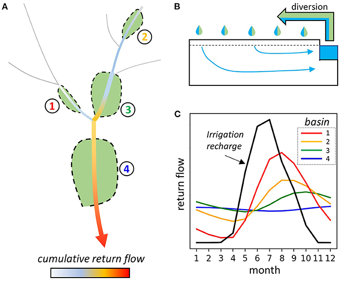
Figure 1. Return flows increase downstream with individual alluvial valleys contributing from lower to higher stream orders within a watershed (A). Irrigation efficiency controls how much diverted water shown by the arrow in (B) becomes recharge (blue fraction). Return flow timing and magnitude is controlled by local basin properties that affect the attenuation and delay of return flow discharge (C).

Integrated over a large basin, return flows can provide substantial quantities of additional baseflow, especially from flood-irrigated land where a large fraction of applied water may not be consumed by crop ET. For example, in the Colorado subbasin where flood irrigation is the primary method of irrigation, mean annual return flows are estimated to be on the order of hundreds of thousands of acre feet per year (~0.1–1 km³) (Colorado Department of Water Resources, 2016). Another example is provided by a recent study by Lonsdale et al. (2020) in Montana where flood irrigation is also common. They found that of the 10.5 million-acre feet (12.95 km³) that are on average diverted annually for irrigation, almost 8 million acre-feet (9.86 km³) are not consumed and likely contribute to groundwater recharge. Local scale estimates of return flows are scarce. Essaid and Caldwell (2017) found that return flows comprised 60–70% of late summer streamflow in the Smith River in Montana, US and Crosa et al. (2006) estimated that return flows accounted for up to 80% of flow in the Amu Darya River in Asia. Additional recharge from stream irrigation can significantly alter the water balance of aquifers (Lonsdale et al., 2020), resulting in long-term increases in groundwater elevation (Scanlon et al., 2005, 2007; Gates et al., 2012) and groundwater discharge to streams (Knight et al., 2005).

The timing and magnitude of return flows are especially pertinent to surface water availability in agricultural regions that rely on streamflow from seasonal snowmelt to supply irrigation, such as the Western United States (US) (Kendy and Bredehoeft, 2006). In snowmelt-dominated hydrologic regimes, large quantities of runoff are generated during the spring and early summer, while groundwater baseflow feeds streamflow after spring runoff subsides and sustains flow until the next season. In this hydrologic regime, diversions during the first half of the growing season (April-June) when flows are plentiful provide return flows that can supplement streamflow during the remainder of the growing season and also into the fall and winter after irrigation has ceased (Venn et al., 2004; Kendy and Bredehoeft, 2006; Essaid and Caldwell, 2017). Because of the heightened importance of return flows providing supplemental flow in regions with highly variable annual streamflow, this study is designed around assessing return flows under conditions of seasonally variable streamflow, irrigation, and natural recharge, representative of a snowmelt hydrographic regime.

Return flows are part of recent debate around whether well-intended efforts over the last few decades to reduce net irrigation water use by switching from lower efficiency flood irrigation to higher efficiency sprinkler or drip methods have resulted unintended negative effects (Ward and Pulido-Velazquez, 2008; Grafton et al., 2018; Lonsdale et al., 2020). A potentially negative unintended effect of increased irrigation efficiency is that the water savings from more efficient irrigation result in reduced aquifer recharge and, correspondingly, reduced return flows. It has been recognized that there may be value in inefficient early season water use when streamflows are plentiful as a means to temporarily store water in alluvial aquifers that can provide a delayed release of return flows to supplement late season streamflow (Van Kirk et al., 2020). Return flows not only increase late season water availability for growers but also municipal and industrial users. They also can help maintain environmental flows necessary for ecological health of river ecology (Kendy and Bredehoeft, 2006; Linstead, 2018). The value of return flows in helping sustain late-season streamflow could increase under climate change as spring snowmelt timing is predicted to occur earlier under warmer climates, prolonging the period of summer and fall low-flows (Ficklin et al., 2013). Return flows are not necessarily entirely beneficial. A potential downside is increased nutrient and salt loading to streams (Isidoro and Quilez, 2003; Gates et al., 2018). Thus, the net benefit of return flows needs to be weighed against harmful effects to aquatic health.

As the need to conjunctively manage surface water and groundwater is recognized to ensure adequate flows for both human and environmental needs (Gorelick and Zheng, 2015; de Graaf et al., 2019), there has been increased effort to incorporate stream-aquifer exchange into water management models and studies. Some examples are the state of Colorado's Stream Simulation Model (StateMod) (Colorado Department of Water Resources, 2016), integrated SW-GW modeling of water resources in the Deschutes Basin, Oregon (Waibel et al., 2013), and in the Arkansas River Basin, Colorado (Whittemore et al., 2006). However, due to the complexity of stream-aquifer dynamics subsurface return flows are either ignored or treated with simplified analytical solutions. While the occurrence and potential importance of irrigation return flows has been recognized for a long time, it is a topic that has not been widely addressed in the literature. Studies on return flows have typically characterized their occurrence in specific study areas (Venn et al., 2004; Kendy and Bredehoeft, 2006; Essaid and Caldwell, 2017) and have not provided generalizable understanding of return flow dynamics. To date, there has not been a sensitivity analysis to generalize return flow processes over a range of common field conditions.

Improved understanding of return flow dynamics can enable more informed water management decision-making. Some examples are the potential cost-benefit tradeoffs of incentivizing more efficient irrigation practices or anticipating how land use changes such as fallowing of irrigated land or urbanization of historical cropland could impact seasonal streamflow. In water management and allocation models that incorporate return flows as part of water availability (Contor, 2009; Colorado Department of Water Resources, 2016; Johnson, 2017), better estimates of return flows can help the models be more representative of water availability provided by return flows.

This study uses detailed groundwater modeling to explore how aquifer properties and boundary conditions influence irrigation return flows. Modeling results are compared to analytically calculated return flows to assess the performance of the analytical solution. We examine how alluvial aquifer size and hydraulic properties influence the timing and magnitude of return flows in alluvial valleys. We also investigate the effects of transient boundary conditions that cannot be accounted for by the analytical solution, such as variable stream stage and transient natural groundwater recharge. Our analysis seeks to provide generalizable insight about controls on return flow dynamics as well as perspective on how analytical approaches perform when compared to numerical models that can account for additional sources of groundwater recharge and variable stream stage.

Methods

Groundwater Modeling

Groundwater modeling of surface water-groundwater exchange in hypothetical irrigated alluvial valleys was done using the United States Geological Survey (USGS) MODFLOW 6 code (Langevin et al., 2017, 2021). Groundwater models representing different alluvial valley sizes and boundary conditions were constructed using the USGS ModelMuse v 4.3 graphical user interface (Winston, 2019, 2020). Boundary conditions and physical properties of these baseline models were then varied using FloPy v 3.3.4, a Python interface for MODFLOW developed by the USGS (Bakker et al., 2016, 2021). FloPy enables script-based automation of large batches of MODFLOW simulations, with the added benefits of reducing user error that can occur when interacting with a graphic user interface and promoting reproducible research by enabling fully transparent Python scripts that document all modeling steps.

The model design is based on a simplified alluvial valley half-width bounded on one side by a valley wall and the other side by a stream (Figure 2). The aquifer is modeled as unconfined with storage defined by specific yield (Sy). The modeling experiments varied alluvial aquifer dimensions (width and depth), aquifer hydraulic conductivity (K), specific yield, and boundary conditions with transient recharge and stream stage. The aquifer is modeled as a 2D slice perpendicular to the river. This follows the simplifying assumption that irrigation occurs over the entire alluvial aquifer footprint, which enables the response from a 2D slice to be representative of the return flow dynamics of the aquifer. In many cases this assumption is reasonable as growers often fully utilize the available arable land in the valley footprint (Examples in SI-1). Following our 2D slice approach, the units of return flow flux are expressed as cubic meters per month per meter of riverbank (m³/month per m of bank).

FIGURE 2

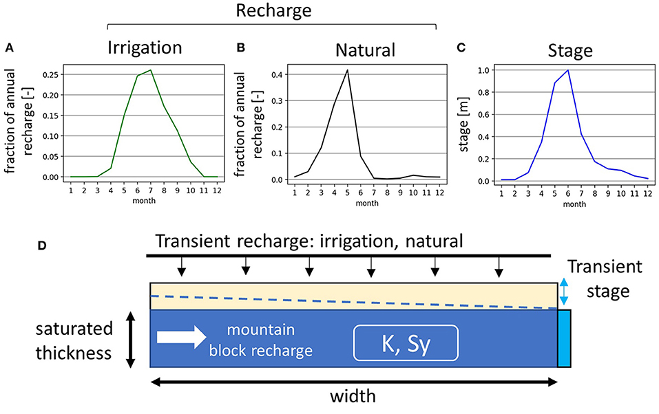
Figure 2. Groundwater model design (D). Transient recharge (flux) boundary conditions are applied to the model top representing irrigation recharge (A) and natural recharge is also included in a subset of simulations (B), and transient stream stage based on normalized snowmelt-dominated stage hydrographs is imposed at the right boundary (C). For model scenarios that include natural recharge, mountain block recharge is represented as constant-flux along the right boundary.

The alluvial aquifer is represented by a 1-layer MODFLOW model with grid cell spacing of 10 m perpendicular to the river and variable cell thickness depending on the modeling scenario. Multilayer models with varying degrees of stream-aquifer penetration were evaluated during study development and were found to have little effect on modeled stream-aquifer fluxes (SI-2). Aquifer saturated thickness is adjusted by moving the elevation of the layer bottom from −10 to −30 m; initial water table elevation and stream stage are set a 0 m, and the land surface (model top) is set a 10 m.

In terms of aquifer properties, simplifying assumptions included isotropic and homogeneous conditions. The stream sediment was assumed to have the same K as the aquifer, a thickness of 1 m, and was assigned a conductance based on model cell area, this further assumes that river width is the same as the cell dimension. To keep the degrees of freedom for the sensitivity analysis manageable, streambed clogging was not varied in these experiments. The effect of a streambed clogging layer was evaluated during model development. A streambed-aquifer K ratio of 1:10 was found to have little effect on monthly stream-aquifer flux (SI-2).

Initial conditions assume equilibrium between the aquifer and river. Boundary conditions include transient river stage at the right-hand boundary of the model, transient recharge along the upper boundary representing irrigation or natural recharge, no flow along the lower boundary representing a large K contrast between the alluvial aquifer and underlying layer, such as bedrock or fine-grained unconsolidated sediment, and either no flow or constant recharge representing mountain block recharge along the left-hand boundary. Transient river stage is defined as a Dirichlet boundary using the RIV package. Recharge (irrigation or natural) is prescribed as a Neumann boundary using the RCH package.

Boundary Conditions

Stream stage, natural recharge, and irrigation recharge boundary conditions (Figure 2) are based on observational and modeling data from the Upper Colorado Basin in the United States. The river stage boundary condition is based on the normalized annual stage pattern for a snowmelt streamflow regime (Figure 2A). The stage boundary condition was created using mean monthly stage data from 24 gauging stations in Colorado [USGS streamflow data: https://waterdata.usgs.gov/co/nwis/rt] (full distribution shown in SI-3). The annual hydrograph is characterized by high stage/flows during April-June and low stage/flows during the rest of the year. The irrigation boundary condition (Figure 2A) is based on monthly irrigation crop water requirement data from 330 irrigation users in Colorado (Colorado Department of Water Resources, 2016, data available in meta-repository for this paper). Like the stream signal, the irrigation pattern is highly seasonal and concentrated during the growing season from April-September, but notably is offset from the stream hydrograph. The third transient boundary condition, applied in a subset of the models, is natural recharge (Figure 2B), which in the Colorado Basin mainly occurs in the spring from the infiltration of snowmelt. The normalized natural recharge boundary condition is based on modeling results in the Upper Colorado Basin (Tillman et al., 2016). For this study, annual natural recharge magnitudes of 10 and 20 cm are used as conservatively high values, in many cases natural recharge in the Western US is substantially lower (Tillman et al., 2016). The last recharge boundary condition in the model is a constant source of mountain block recharge. Annual mountain block recharge is scaled to 25 and 50% of annual surficial natural recharge, based on ratios found in regional modeling studies that incorporate mountain block recharge (Markovich et al., 2019).

Analytical Representation of Return Flows

The analytical solution used to calculate groundwater discharge (return flows) to a stream from irrigation recharge is based on the formulation of stream depletion from a pumping well at a distance from a river presented by Glover and Balmer (1954). The equation used in this study, presented by Knight et al. (2005), uses on an infinite series of paired image wells to account for the effect of the alluvial valley boundary (Equation #1).

$\begin{array}{ll}f\left(a,c,t\right)=-\left\{erfc\left(\frac{a}{{2\left(Dt\right)}^{1/2}}\right)+{\displaystyle \sum _{n=1}^{\infty }}{\left(-1\right)}^{n+1}\left[erfc\left(\frac{2nc-a}{2{\left(Dt\right)}^{1/2}}\right)-erfc\left(\frac{2nc+a}{2{\left(Dt\right)}^{1/2}}\right)\right]\right\}& (1)\end{array}$

Where f is the fraction of stream depletion (the opposite of return flow) at time t, a is the distance between the pumping well and stream, c is the distance from the stream to the valley boundary, and D is the hydraulic diffusivity of the aquifer (K^*thickness/Sy).

Reversing the sign of Equation 1 has the physical meaning of recharging the aquifer at a distance rather than pumping. With the sign reversed, Equation 1 describes the unit response function of aquifer discharge to a stream resulting from the initiation of a continuous point recharge source. The convention is to place the recharge point source at the midpoint of the irrigated acreage's distance from the stream (Knight et al., 2005). This study assumes that the entire alluvial valley is irrigated so the recharge point source is located at the mid-point of the alluvial valley width, that is a = ½^*c. Our analysis uses the first six terms of the infinite series as additional terms make insignificant contributions.

Some additional steps are required to use Equation 1 for calculating transient return flows resulting from a transient recharge signal. The first step is to calculate the unit response time series for a given set of aquifer properties (width, depth, K, Sy). The unit response time series is then used to calculate the lagged response function for discharge (return flow) to the stream during and following a recharge stress period of defined length. A 1-month stress period is used since we are interested in estimating monthly return flows resulting from irrigation. The discrete recharge stress period is produced by initiating unit pumping at the recharge point after a month of unit recharge. Example results for return flow during and after a 1-month stress period are shown in Figure 3A. The time series of return flows resulting from the 1-month stress period is then integrated at 30-day increments to produce the monthly response function (Figure 3B), which describes the fraction of recharge from Month i that returns to the stream in Month i and each following month. For example, the monthly response curve in Figure 3B shows that roughly 10% of the total recharge returns to the stream in the same month of irrigation (month = 1), a little over 20% returns in the month following the irrigation recharge, and about 15% returns in the second month following the irrigation recharge. The lagged response function can then be applied to a monthly time series of recharge (Figure 3C) to generate lagged return flows produced by each month of recharge (Figure 3D). Finally, the return flow time series can be calculated by superposing the lagged response function for each month (Figure 3E). This procedure was executed for the three different aquifer widths and four K-values to produce analytical return flows to compare to the modeling results.

FIGURE 3

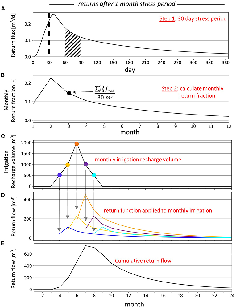
Figure 3. Example of the analytical return flow methodology. The first step is to create the daily return flow fraction for a 30-day stress period (A). The end of the stress period is denoted by the dashed line. The daily return fraction is then integrated in 30-day intervals (ex. hash marked region in subplot a) and divided by 30 m³ (30 days of unit recharge) to generate the monthly return flow fraction (B). The monthly return fraction is then used to generate the lagged returns for each month of a irrigation recharge time series (C,D). The individual return flow time series for each month of recharge can then be summed to produce the cumulative return flow time series (E).

Experiment Groups

This study contains three sets of experiment groups, each designed to test the interaction of different factors affecting return flows (Table 1). The effect of the physical dimensions of the alluvial valley on return flows is explored by considering three valley widths (500, 1,000, 2,000 m) and three aquifer saturated thicknesses (10, 20, 30 m). The control of hydraulic properties on irrigation return flow dynamics is explored by using four K-values ranging from 3 to 100 m/d (3, 10, 30, 100 m/d) and two values of specific yield (0.2, 0.3). These values are typical of alluvial aquifers in mountainous alluvial valleys in Western Colorado (Colorado Department of Water Resources, 2016; United States Forest Service, 2018; Newman et al., 2021). The effects of stage and recharge boundary conditions are explored by using four different magnitudes of stream stage amplitude (0, 0.5, 1, and 2 m), three values of net annual irrigation recharge (10, 20, 30 cm), two magnitudes of surficial natural recharge (10 and 20 cm) each with two mountain block recharge magnitudes (25, 50%).

TABLE 1

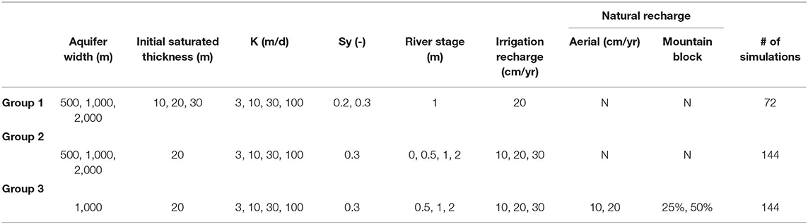
Table 1. Parameter and boundary condition settings for the three experiment groups.

Group 1 examines the effect of aquifer saturated thickness, specific yield, and hydraulic conductivity across three aquifer widths. In Group 1, river stage hydrograph has an amplitude of 1 m and the irrigation recharge signal is scaled to 20 cm of annual recharge. In Group 2, initial aquifer saturated thickness and specific yield are held constant to explore the effect of different stream stage amplitudes and irrigation recharge magnitudes. Group 3 introduces natural recharge to test how natural aquifer recharge affects return flow dynamics.

To explore temporal dynamics, groundwater simulations for each experiment group are run for 11 years, with the first 10 having the same repeating boundary conditions and the 11th representing a drought where the stream stage and natural recharge are reduced by 50% and no irrigation representing fallowing conditions. Also explored is how a strong, single, single-year drought impacts the system. All the experiment groups, and corresponding analytical results, present return flows in the 10th year of the simulation when the stream-aquifer systems have achieved equilibrium. The time needed to reach equilibrium increases for wider aquifers and for lower hydraulic conductivities. The spin up period ensures the results are more representative of conditions in irrigated regions where irrigation has been occurring for significant periods of time.

Calculating Return Flows From Modeling Results

Return flows for a given scenario, i.e., how much additional discharge to the stream occurs due to irrigation recharge, are calculated by comparing the stream-aquifer flux from the given scenario to a baseline reference simulation where all other boundary conditions are present except irrigation. Thus, every irrigation scenario in this study (Table 1) has a corresponding baseline simulation. The approach of using irrigation and baseline simulations to isolate the effect of irrigation is illustrated in Figure 4, which shows the stream-aquifer flux with (Figure 4B) and without irrigation (Figure 4A). The sign convention in Figure 4 and throughout the paper is positive flux represents flow out of the aquifer and negative flux represents flow into the aquifer. Differencing the stream-aquifer exchange time series from the baseline reveals the additional groundwater flux to the stream from irrigation (Figure 4D). Exchange between the aquifer and river is controlled by both the aquifer head and river stage. Periods where the river stage is higher than that of the adjacent aquifer result in flow from the river to the aquifer, as shown in Figures 4A,B. It should also be appreciated that any increase in river stage, even if it is not substantial enough to cause a flow reversal, reduces groundwater flow out of the aquifer (baseflow). Interestingly, it can be seen that irrigation recharge reduces natural recharge from stream-aquifer exchange (Figure 4C). This phenomenon is not assessed in this study but is an interesting implication that irrigation recharge can alter natural stage-induced seasonal recharge of alluvial aquifers.

FIGURE 4

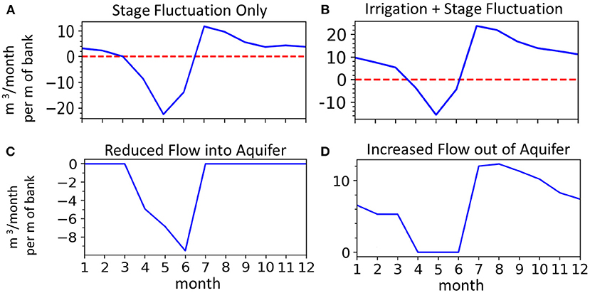
Figure 4. Example model results showing SW-GW flux across the stream-aquifer boundary for the baseline case of stage fluctuation (A) and with both irrigation recharge and stage fluctuation (B). Compared to the baseline case, irrigation recharge reduces stream-aquifer exchange during April-June (C) and increases groundwater discharge (return flows) during the rest of the year (D).

Results

Insights From Analytical Solution

Even though the analytical solution is an abstraction of the physical return flow process, as it represents irrigation recharge at a single recharge point at some offset distance from the stream rather than infiltration occurring over the land surface, it provides first-order insight into how aquifer width and hydraulic conductivity jointly influence return flow dynamics (Figure 5). These results are for a Sy of 0.3 and thickness of 20 m. The results present the monthly irrigation recharge (black line) in the same units as the return flow results (m³/m of bank per month) so a direct comparison can be made between the irrigation recharge and resulting return flow. The analytical results show that wider alluvial aquifers and lower hydraulic conductivities produce more lagged and attenuated return flows. Notably, the highest K value (100 m/d) for the narrowest aquifer (500 m) is the only case where the return flow response is similar in timing and magnitude to the irrigation recharge signal. In all other cases, the return flows are attenuated and offset by multiple months. For a given aquifer width, the return flow peak is more delayed as K decreases. For example, the peak return flow timing for the 500 m aquifer occurring in July for K = 100 m/d is shifted to September-October for K = 3 m/d. In addition to delaying return flow timing, lower K also increases the constant baseflow component of the return flows and lowers the amplitude of the seasonal fluctuation.

FIGURE 5

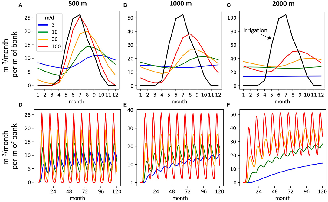
Figure 5. Analytical return flows in year 10 (A–C) and return flow time series showing equilibrium time scales for the three aquifer widths and K-values (D–F).

The analytical results also demonstrate how aquifer width and K control the equilibration time scale for the return flow. Depending on the aquifer width and K-value, equilibrium can take as little as 1 year to over a decade. All four K-values reach equilibrium within 4 years for the 500 m wide aquifer, and for the 1,000 m wide aquifer all but the 3 m/d scenario also reach equilibrium after 4 years. The only two cases that do not achieve equilibrium after 10 years are the 3 and 10 m/d scenarios for the 2,000 m wide aquifer (Figure 5F, blue and green curves), evidenced by their curves not completely asymptotically leveling off. The time required for a given aquifer to equilibrate indicates how rapidly a change in conditions will affect the return flows. An aquifer that equilibrates in a year or two will respond rapidly to a change in conditions (irrigation magnitude for example), whereas an aquifer that has a long equilibration timescale, such as the lower K conditions in the 2,000 m wide aquifer, will take longer to fully adjust to new external forcings. It should be noted that the analytical solution is agnostic to the individual contributions of K, b, and Sy and that their combined effects on the hydraulic diffusivity (plus aquifer width) controls the return flow response.

Group 1: Varied Saturated Thickness and Specific Yield

The simulations for Group 1 isolate the effect of alluvial aquifer saturated thickness and specific yield by using one irrigation recharge magnitude (20 cm/yr) and one stage amplitude (1 m). For each aquifer width (columns) and K (rows), return flows are shown for three initial saturated thickness, each with two Sy values, as summarized in Table 1. All else equal, larger saturated thickness generate larger return flow magnitudes (Figure 6). However, this effect is not uniform across the various combinations of valley width and K. For example, there are negligible differences between the three aquifer thicknesses for the 500 m wide aquifer with a K of 100 m/d (Figure 6J), while the differences between the 10 and 30 m thickness for the 2,000 m wide aquifer with a K of 10 m/d are on the order of 30–40%. Specific yield (dotted vs. solid lines in Figure 6) defines how much a unit of aquifer recharge increases the water table elevation. For the same initial saturated thickness, lower Sy results in larger return flows during the later summer to fall period.

FIGURE 6

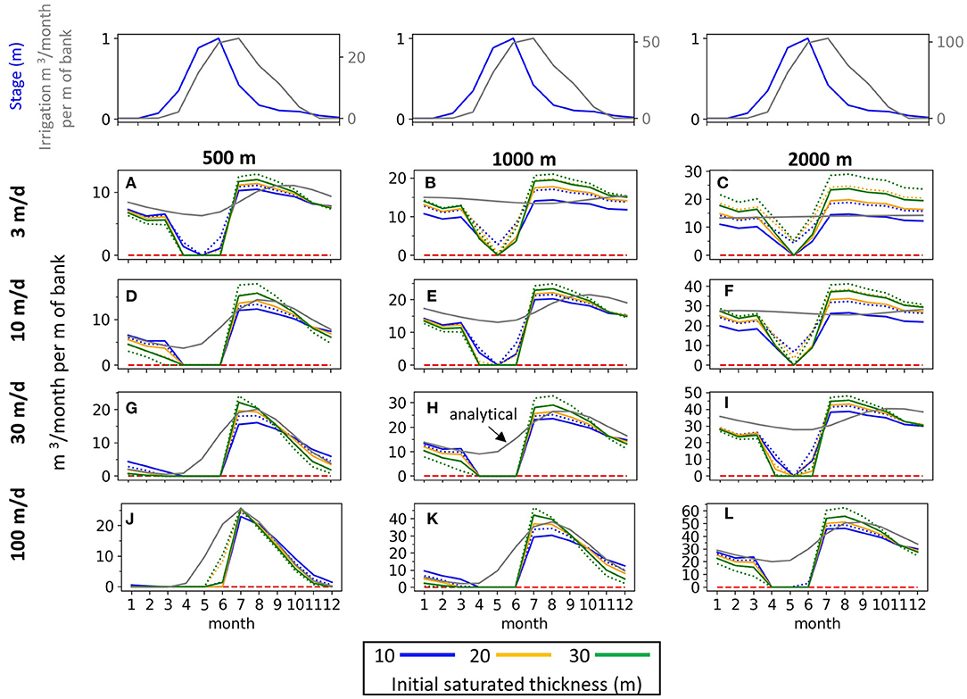
Figure 6. Return flow results for Group 1. The six return flow curves within each combination of aquifer width (columns) and K (rows) correspond to three different initial aquifer saturated thicknesses (colors) and two specific yield values for each saturated thickness (dashed = Sy 0.2, solid = Sy 0.3). Stream stage and recharge boundary conditions are plotted above the return flow results to provide reference of how return flow timing relates to the boundary conditions. Gray line shows the analytical solution with an aquifer thickness of 20 m and Sy = 0.3.

Comparison to Analytical Solution

The gray lines in Figure 6 show the analytical solution corresponding to the scenarios with a 20 m thick aquifer with a Sy of 0.3 (solid orange line). The results for the orange solid line are illustrative of general deviations of the analytical solution from the modeled return flows for each aquifer width and K scenario (plotting the corresponding analytical solution for all six combinations of b and Sy would make Figure 6 uninterpretable).

Most significantly, the modeling-analytical comparison shows that return flows are suppressed or entirely absent for the April-June period during rising limb of the snowmelt hydrograph. During this period, the river stage counters the head gradient between the aquifer and river. In the cases where return flows are zero during the April-June period (ex. Figure 6H), the stream is recharging the aquifer and there is no groundwater outflow, while positive return flows during this period (ex. Figure 6B) indicate that the stream stage is not causing a flow reversal but is reducing the return flow flux. The spring stream stage increase causes groundwater levels to increase along the stream-aquifer boundary and throughout the alluvial aquifer as the irrigation recharge is unable to outflow to the river. The analytical solution requires the assumption of a constant stream stage and therefore cannot account for the reduction in return flows from the stream stage increase. This leads to the analytical solution overestimating return flows during the early growing season, with the degree of error varying depending on aquifer width and K. Also of note, is the error between the analytical results and the modeled return flows during other parts of the year with the general tendency to underestimate return flows during the July-September period (Figures 6A–C,E,F,I) and to overestimate them during October-March (Figures 6A,B,E,I).

Return Flows During Drought Year

Return flows during a hypothetical drought, the 11th year of the simulation, demonstrate how aquifer width, K, depth, and Sy influence the cumulative carry-over effect of irrigation recharge from previous growing seasons. Because there is no irrigation recharge during the hypothetical drought year, all return flows are sourced from accumulated aquifer storage from previous years.

The processes of irrigation recharge increasing aquifer storage was not discussed in the Group 1 results but is essential to understanding return flows during the drought year. Depending on the aquifer width and K, the annual irrigation recharge cannot fully discharge to the stream before the next irrigation season, resulting in an increase in aquifer storage (increase in water table elevation). The imbalance between aquifer recharge and discharge is greater for wider aquifers and lower K-values, resulting in more stored irrigation recharge to contribute to return flows during the drought year.

The effect of aquifer width and K can be seen by comparing return flows for the same width (columns) or for different aquifer widths with the same K (rows) (Figure 7). The decay of the return flow curves over the drought year represent the draining of accumulated storage. The stream stage fluctuation for the drought scenario has a peak amplitude of 0.5 m instead of 1 m to represent reduced streamflow (and stage) during a drought. While half the amplitude, the drought snowmelt hydrograph still reduces return flows during April-June; in the case of a drought, the spring snowmelt hydrograph has the beneficial effect of delaying discharge from the alluvial aquifer so more of the outflow occurs during the later summer months when stream flows are more diminished.

FIGURE 7

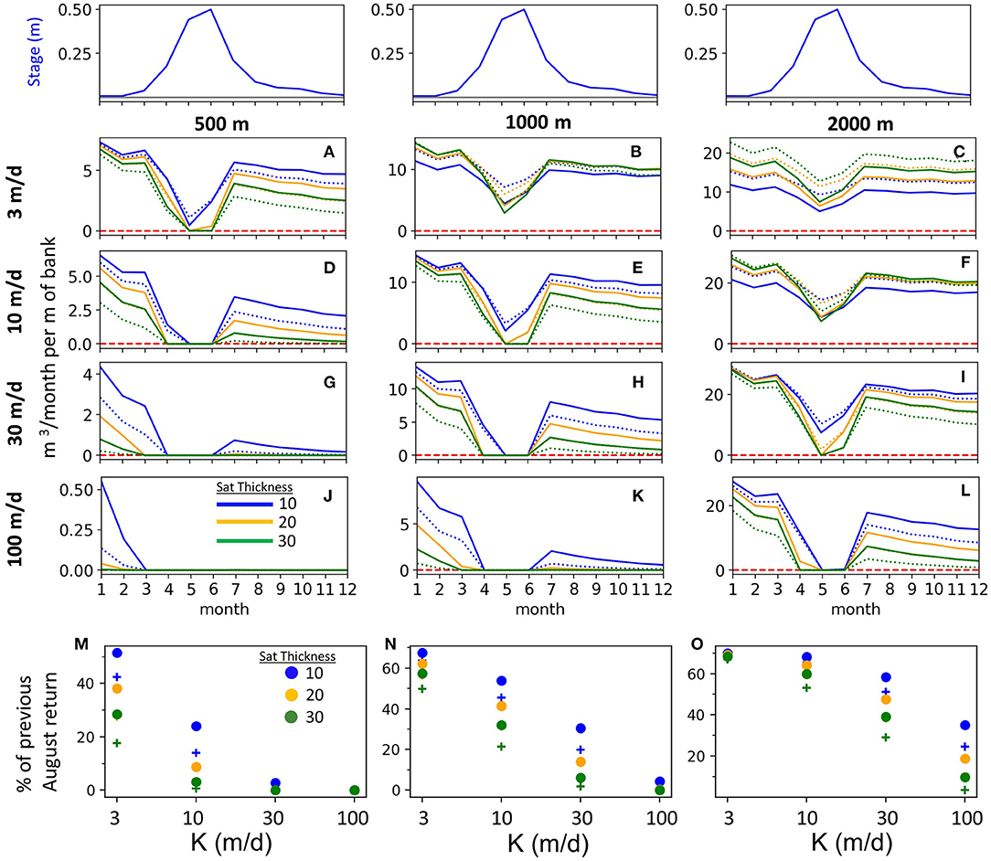
Figure 7. Return flows during the drought year (A–L) for three initial aquifer saturated thicknesses (colors) and two specific yields (dashed = Sy 0.2, solid = Sy 0.3). Return flows for August of the drought year are compared to August in the previous year and expressed as a percentage of the previous year's monthly return flow for August (M–O). Plus sign designates Sy = 0.2 where dot is for Sy = 0.3.

To summarize the combined effects of aquifer width, K, initial saturated thickness, and Sy on carry-over return flows during the drought year, August return flows during the drought are compared to the previous year return flows (Figures 7M–O). Return flows during this critical late-summer low flow period are expressed as the percentage of the previous August's return flows. The percent varies widely from as high as 70–0%. Narrower alluvial aquifers with higher Ks have less of a buffering capacity during a drought year when irrigation recharge is reduced or in the case of this extreme example, are entirely absent. Notably, return flows decline less for wider aquifers. For example, the August return flows for the 500 m wide aquifer with K = 10 m/d range from ~0–25% of the previous August (Figure 7M), while the fraction for the 2,000 m wide aquifer with K = 10 m/d is 50–70% (Figure 7O). Greater aquifer saturated thickness results in more rapid decline in drought year return flows. Thicker (more transmissive) aquifers accumulate less carry over irrigation storage because they have a higher hydraulic diffusivity (transmissivity/Sy) than a thinner aquifer with the same K, which allows them to return irrigation recharge more rapidly to the stream than a thinner aquifer. The same relationship can be understood for the lower specific yield of 0.2 (plus signs) having greater reductions in drought return flows than the 0.3 specific yield (circles).

Group 2: Varied Stream Stage and Irrigation Recharge

The first experiment group revealed that the rising limb of the snowmelt hydrograph during the spring and early summer can reduce or prevent return flow. To investigate this further, the second experiment group examines the interaction between stream stage amplitude and irrigation recharge for four different stream boundary conditions and three different irrigation recharge intensities. The stream stage and irrigation patterns are generated from the normalized annual patterns (Figures 2A,C). The stream stage patterns have amplitudes of 0, 0.5, 1, and 2 m; the steady stream stage (amplitude = 0) is considered as a reference for examining how varying amounts of stream fluctuation influence return flow dynamics. The three irrigation recharge magnitudes are 10, 20, and 30 cm/yr.

For all three irrigation recharge magnitudes, stream fluctuations prevent or greatly reduce return flows during the April-June period (Figure 8). The 2 m stage amplitude prevents April-June return flows for all cases. For the wider aquifers and lower K scenarios (Figures 8B,C,E,F) there are some April-June return flows for the 0.5 (dotted lines) and 1 m (dashed lines) amplitudes. However, the April-June return flows that do occur are all a small fraction of what would occur if the stream stage were constant (solid line). A surprising result from these simulations is that a snowmelt hydrograph with a seasonal amplitude as small as 0.5 m can mostly suppress irrigation return flows during the rising limb of the hydrograph (April-June). Different recharge magnitudes proportionally increase or decrease the return flow magnitude but do not alter the timing of the return flow peak for a given aquifer width and K condition. Larger recharge magnitudes proportionally increase return flows and increase groundwater discharge to streams throughout the entire low-flow period from August to February. For example, considering the 2,000 m wide aquifer with K = 100 m/d, an irrigator that recharges the aquifer by 30 cm per year generates three times as much baseflow during the later summer, fall, and winter as an irrigator who only recharges the same aquifer by 10 cm per year (Figure 8L).

FIGURE 8

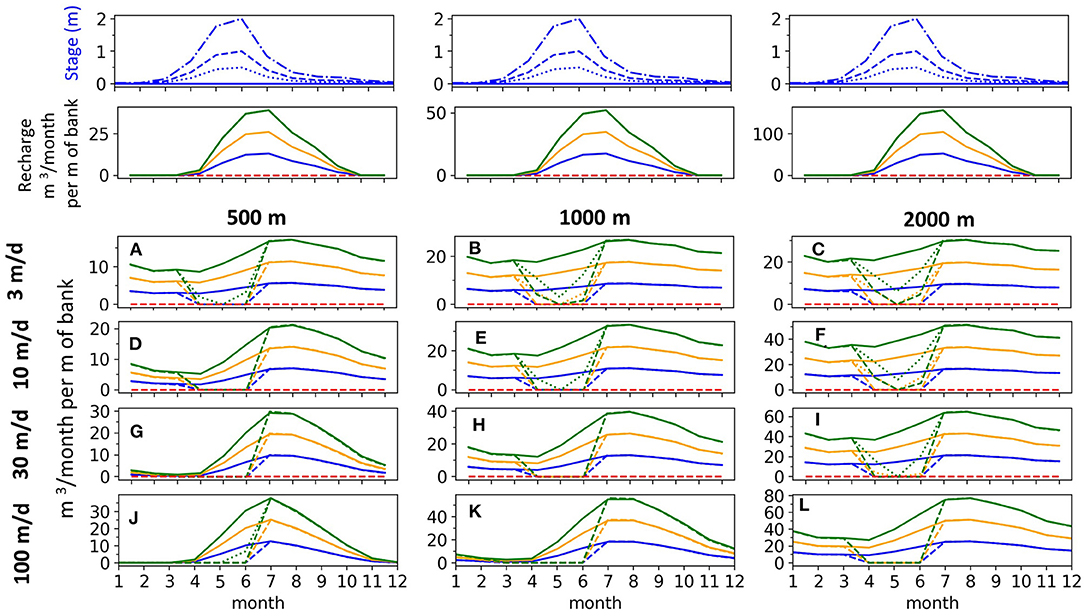
Figure 8. Return flows from three different recharge magnitudes (colors) and four different stream stages (denoted by line style corresponding to the four stream hydrographs in the top row). (A,D,G,J) Are for 500 m width, (B,E,H,K) are for 1000 m width, and (C,F,I,L) are for 2000 m width.

Group 3: Varied Natural Recharge, Stream Stage, and Irrigation Recharge

The final group of simulations examine how return flows are affected by the addition of a natural groundwater recharge pattern. Specifically, the objective of this simulation group is to explore whether additional natural recharge can create sufficient gaining conditions in the aquifer to overcome the stream stage boundary condition that prevents or greatly reduces groundwater discharge during the rising stage of the spring hydrograph. The natural recharge pattern in these simulations is representative of alluvial valleys that receive most of their recharge from spring snowmelt, such as in mountainous regions in the Western US.

Due to the number of parameter combinations, only one aquifer width of 1,000 m is considered in this simulation group. The simulations span four K-values, three stage amplitudes (0.5, 1, 2 m), three annual irrigation recharge magnitudes (10, 20, 30 cm), and four natural recharge patterns that are defined by 10 cm (Figure 9 second row, gray) and 20 cm (Figure 9 second row, black) of annual recharge representing surficial recharge, each with two values of additional basin fill recharge that is a constant monthly flux along the alluvial valley boundary (Figure 2) that totals 25% (solid) and 50% (dashed) of the annual surficial recharge.

FIGURE 9

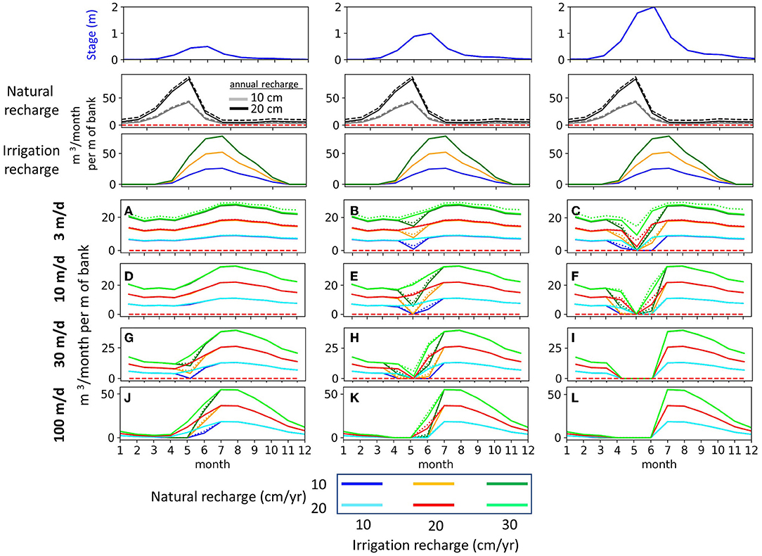
Figure 9. Return flow for simulation Group 3. The first three rows show, respectively, the corresponding transient stage, natural recharge, and irrigation recharge patterns. The three irrigation recharge magnitudes are denoted by the green/lime (30 cm/yr), orange/red (20 cm/yr), and blue/cyan (10 cm/yr) with each color pair corresponding to the two different natural recharge magnitudes as shown in the legend. The dotted vs. solid lines in subplots A-L denote the two constant mountain block recharge flux rates (dashed = 50% and solid = 25% of net annual recharge). Subplots (A,D,G,J) correspond are for a 0.5 m stage amplitude, (B,E,H,K) are for 1 m amplitude, and (C,F,I,L) are for 2 m amplitude.

The effect of natural recharge on April-June return flows varies widely depending on the river stage amplitude and aquifer K (Figure 9). With the addition of natural recharge, return flows are mostly unchanged during the April-June period for the 0.5 m stage case (Figures 9A,D,G,J). There is notably almost no difference in return flow results for the two constant mountain block recharge fluxes (dotted vs. solid lines in the return flow plots). However, the two magnitudes of natural surficial recharge (10 and 20 cm/yr) do have differing effects on whether return flows occur during the period of rising stage in April-June. For example, the 20 cm natural recharge pattern results in return flows being unchanged for the K = 3 and 10 m/d conditions when the stage fluctuation is 1 m (Figures 9B,E). Return flows are absent or greatly reduced during April–June for the 2 m stage amplitude (Figures 9C,F,I,L), showing that even these large quantities of natural recharge do not yield additional groundwater discharge from return flows during the rising limb of the snow melt hydrograph. For all the added complexity introduced in this third simulation group, the overall pattern of return flows for the three irrigation magnitudes closely resembles the results from Group 2 (Figure 8) where there was no natural recharge. Most significantly, the different natural recharge magnitudes do not change the return flow timing or magnitude during the annual hydrograph recession (July–February), evidenced by the fact that the return flow pairs for each irrigation magnitude completely overlap during this period (Figures 9A–L). Thus, natural recharge can change return flows during the spring and early summer but has no influence on their timing during the rest of the year, which is when their occurrence provides critical supplementary streamflow.

Discussion

Control of Alluvial Aquifer Width, K, and Irrigation Recharge on Seasonality of Return Flows

From a water management perspective, it is valuable to understand whether return flows tend to be highly seasonal or provide more consistent year-round supplemental flow to streams. To show how the seasonality of return flows is controlled by aquifer width, K, and irrigation recharge (ex. efficiency differences), the maximum monthly return flow volume (m³/m of bank) is compared to the return flow volume in February for the entire range of Group 2 scenarios (Figure 10). February is selected to be representative of the long-term baseflow contribution from return flows as it is several months since irrigation has ceased and only 2 months before irrigation resumes. Also, of relevance, streamflow is at or near its annual minimum during February (Figure 2C). The 1:1 line in Figure 10 is a reference for how consistent return flows are annually; the closer February return flow volume is to the annual maximum, the less seasonally-variable the return flow pattern. There is a consistent pattern across the three aquifer widths that lower K aquifers generate more stable return flows (Figure 10). Also, as aquifer width increases return flows have a larger baseflow component and plot closer to the 1:1 line (Figure 10A compared to 10C).

FIGURE 10

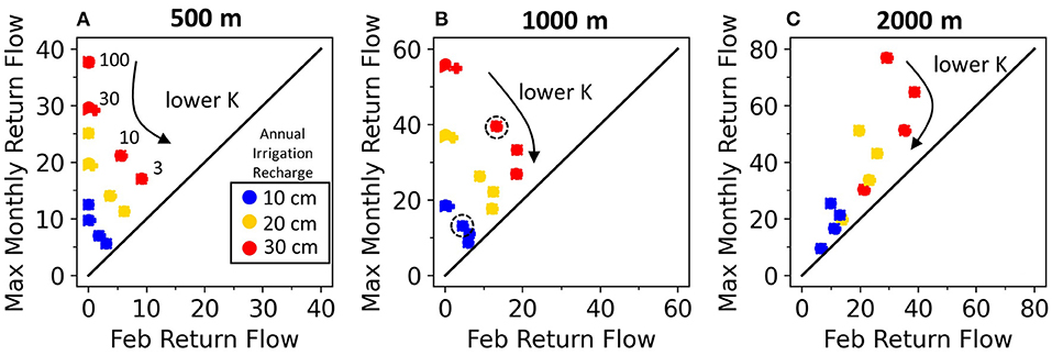
Figure 10. Ratio of maximum monthly return flow to February return flow (representative of the long-term baseflow component). Individual values are organized by color (annual irrigation recharge), hydraulic conductivity (annotated for each graph) and by aquifer width (A–C).

The three different irrigation recharge magnitudes presented in Figure 10 can be used to interpret how a change in irrigation efficiency (increase or decrease in annual recharge) would affect return flow characteristics. For example, if irrigation in a 1,000 m wide alluvial valley with a K of 10 m/d (Figure 10B) is converted from flood to sprinkler irrigation, hypothetically reducing annual recharge from 30 cm (red) to 10 cm (blue), the affect would be to reduce the maximum monthly return flows from 40 to 13 m³/m per month and the long-term baseflow from 15 to 5 m³/m per month. This example is illustrated in Figure 10B by the two circled points.

Accuracy of Analytical Solution During Late Summer and Winter

The modeling results reveal that the analytical solution performs poorly during the rising limb of the snowmelt hydrograph (Figures 6, 8, 9). Another important consideration is the accuracy of the analytical solution for estimating the late season and baseflow streamflow contributions of return flows. The analytical performance for Group 2 scenarios is assessed by comparing analytical and model return flows over the July-September and December-February periods, with the difference over each 3-month period quantified in both absolute and percentage terms (Figure 11). The differences are calculated by summing analytical and modeled return flows for each 3-month period; thus, the reported values are the net over or underestimate of cumulative return flows over each 3-month comparison window.

FIGURE 11

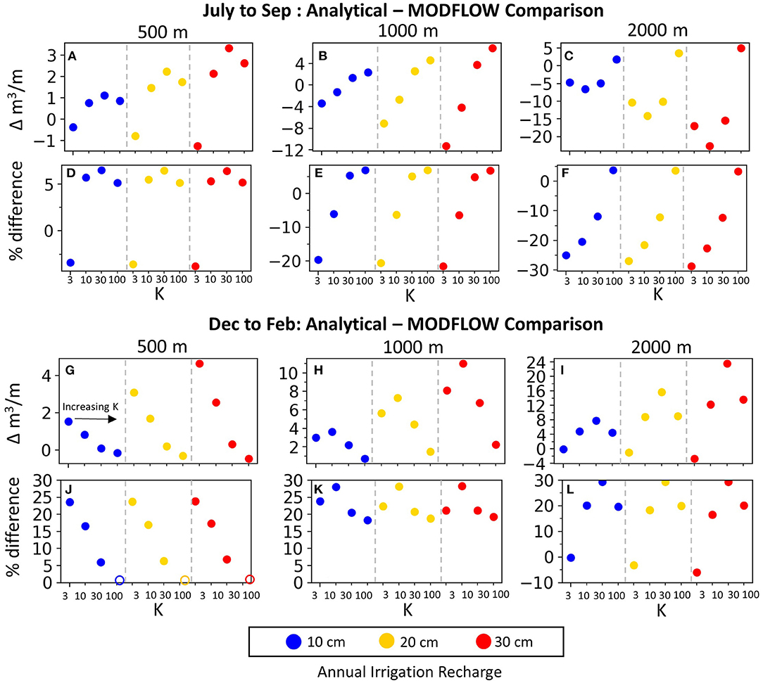
Figure 11. Assessment of analytical return flows against modeled return flows for July-September (A–F) and December-February (G–L). Within each subplot, each irrigation recharge value is grouped by annual irrigation recharge (indicated by different colors) and aquifer K, as annotated in (G) and indicated on the x-axis. The open circles in (J) are because the actual percentage difference is off of the plot (−700%), but because the absolute difference for these three cases is very close to zero (G), we plotted the % difference near zero so the other values in (J) would be legible.

The detailed analysis in Figure 11 supports the general observation made in the results section that the analytical solution tends to overestimate winter return flows (December-February); the only two exceptions are for the K = 3 m/d conditions in the 2,000 m wide aquifer (Figure 11L). During the winter period, the overestimates are up to 30% and frequently between 15 and 25%. However, in absolute terms, the overestimates are larger for wider alluvial aquifers (Figure 11I) than narrower ones (Figure 11G). Unlike the winter period, there is not a consistent pattern of over or underestimates during the summer and early fall (Figures 8A–F). During July-September the analytical solution overestimates or underestimates return flows depending on the aquifer width and K, but notably not irrigation recharge. The analytical solution overestimates July-September return flows in the 500 m wide aquifer for the all but the lowest K (Figures 11A,D), for the two higher K-values in the 1,000 m wide aquifer (Figures 11B,E), and only for the highest K in the 2,000 m wide aquifer (Figures 11C,F). However, the magnitudes of overestimates are all <10% while the underestimates which range from 5 to 30%, with larger underestimates for wider aquifers with lower Ks.

Implications for Water Management

The modeling results provide insights relevant to multiple aspects of water management. Perhaps most notably, and to our knowledge not reported in previous studies, is our finding that the analytical solution can overestimate return flows during the rising limb of the spring snowmelt hydrograph because it cannot account for the effect stream stage fluctuations have on return flows (Figures 6, 7, 9). From a water supply management perspective, it is better that the analytical solution performs poorly during the first half of the growing season when streamflows are generally high, than during the July-October period when streamflows are declining and there is still high water demand for irrigation. The tendency for the analytical solution to either underestimate or only slightly overestimate (<10%) return flows during the July-September period (Figure 11) means that it is not over-representing late season water availability from return flows.

Aquifers that have the capacity to accumulate and store irrigation recharge can provide supplemental return flow during years when irrigation recharge is reduced or even when it is absent (Figure 7). While not a focus of this study, there is the potential to conjunctively manage alluvial aquifers that have significant carry-over storage [favored by wider and lower K (Figure 7)] in a scheme where crops are generally irrigated from surface water diversions, but during a drought, crop water demand can be supplemented by groundwater wells that draw from accumulated storage. A modeling analysis would help uncover the costs and benefits of banking irrigation recharge in alluvial aquifers to increase resilience during drought conditions.

While return flows in this study are only examined in the context of water quantity, it has been shown that they can impact stream water quality, both chemistry (Knight et al., 2005; Causapé et al., 2006) and temperature (Essaid and Caldwell, 2017; Alger et al., 2021). Water quality concerns from return flows relate to increasing salt (Knight et al., 2005) and nitrate (Causapé et al., 2006) loads to streams. In terms of temperature, return flows have been shown to buffer stream temperatures during summer low flow periods (Essaid and Caldwell, 2017; Alger et al., 2021). The overall benefit of return flows on stream temperature must be balanced against the negative impacts that reduced flows due to diversions can have on stream temperature (Bunn and Arthington, 2002; Miller et al., 2007). Our modeling results show that in different settings alluvial aquifers can have quite different magnitudes and seasonal variability of return flows. The timing and magnitude of return flows in relation to streamflow controls the degree to which they can impact stream water quality (positively or negatively).

Limitations and Future Work

This study makes several necessary simplifying assumptions about the hydrology and irrigation practices in alluvial valleys. First, we make the simplifying assumption that irrigation occurs over the entire alluvial aquifer extent. In many cases this assumption is reasonable as growers often fully utilize the available arable land in the valley footprint (Examples in SI-1). However, for cases where only a fraction of the alluvial valley footprint is irrigated, it should be understood that return flows could be more delayed and attenuated than the results in this study. Another assumption is that groundwater flow is predominantly perpendicular to the stream, which enables us to model the return flows in alluvial aquifers as perpendicular slices of the river-aquifer system. Exploratory modeling (SI-4) shows that groundwater flow remains mostly perpendicular to the stream over a range of down-valley slope, and that longitudinal, down-valley flow negligibly effects return flow timing when the valley footprint is fully irrigated.

In our models, it is assumed irrigation is entirely sourced from surface water diversions. This is a reasonable assumption for irrigation practices throughout the Mountain West (Colorado, Wyoming, Montana, Utah, Idaho, Oregon, Washington) where surface water still provides most of the water for irrigation (Dieter et al., 2018). In alluvial valleys where groundwater provides significant amounts of irrigation, groundwater pumping could capture irrigation recharge and therefore reduce return flows as well as potentially reducing natural groundwater baseflow (de Graaf et al., 2019). Future studies could examine how different ratios of surface water diversions and groundwater pumping and spatial configurations of wells relative to the stream and alluvial aquifer footprint, impact return flow and natural groundwater baseflow dynamics.

Our study assumes neutral or gaining groundwater conditions, which for much of the Mountain West is a reasonable assumption as supported by CONUS stream-groundwater configuration mapping by Jasechko et al. (2021). Our models did not consider alluvial aquifers with losing or disconnected water tables, as return flows would not be expected to be a sizeable fraction of irrigation recharge in such settings.

Due to the limited number of scenarios we could investigate and manageably present, we only used one stage (Figure 2A) and one irrigation (Figure 2C) pattern, whose magnitudes were varied to represent different snowmelt hydrograph stage fluctuations and irrigation recharge conditions. The irrigation and stage patterns are broadly representative of conditions throughout the US Mountain West, where the growing season occurs during April–September and streamflow is controlled by the spring snowmelt. In other locations there could be different timing between the irrigation recharge and annual steam stage fluctuations. Our modeling shows that the interaction of the recharge signal with stream stage can alter the timing and magnitude of return flows. In other streamflow regimes we would expect that periods of seasonally high stage could reduce or halt return flows for some period. A potential avenue for future work would be to perform a global sensitivity analyses (i.e., Saltelli et al., 2019) assessing how aquifer properties (dimensions, K, Sy), irrigation patterns (timing and intensity), natural recharge (timing and intensity), and stream fluctuation (timing and magnitude of hydrograph) interact to influence the timing and magnitude of return flows. Such an analysis could provide valuable insight about interactions between irrigation recharge and stream stage and how aquifer properties modulate the sensitivity to these two signals.

Conclusions

This study used groundwater modeling to gain insight into controls on irrigation return flows. Three groups of sensitivity experiments were used to explore how a wide range of factors that include alluvial aquifer geometry, hydrological properties, irrigation recharge, stream stage, and natural recharge influence return flow dynamics. Stream stage fluctuations were found to suppress return flows during the rising limb of the snowmelt hydrograph, suggesting that return flows in many Western US streams may be reduced during the spring snowmelt runoff period. Wider alluvial valleys with lower K sediments result in more attenuated return flows that provide more constant year-round baseflow, while narrower alluvial aquifers with higher K sediments generate more seasonally variable return flows concentrated during the summer and early fall. If alluvial aquifer K is <3 m/d, our modeling suggests that there would be very little seasonal variation in return flow magnitude (Figure 10). Similarly, wide alluvial valleys whose irrigated area extends many kilometers from the river are also expected to have less variable return flows (Figure 10). Comparisons of modeled return flows to analytical approximations show that the analytical solution overestimates return flows during the rising limb of the snowmelt hydrograph because it cannot account for stage variations countering groundwater outflow. The analytical solution was found to underestimate or only slightly overestimate return flows during the late summer and fall period, which means that it is not over-representing return flow contributions during this critical low-flow period. These results provide scientists and water managers new perspective on how local, site-specific factors influence return flow behavior, and awareness about possible shortcomings of analytical solutions that are commonly used for estimating return flow contributions to streamflow.

Data Availability Statement

The datasets presented in this study can be found in online repositories. The names of the repository/repositories and accession number(s) can be found at: https://github.com/IMMM-SFA/ferencz-tidwell_2022_frontiers.

Author Contributions

SF performed the modeling and data analysis and wrote the draft of the paper. All authors contributed to the experimental design and conceptualization and edited and revised the document throughout. All authors contributed to the article and approved the submitted version.

Funding

This research was supported by the U.S. Department of Energy, Office of Science, as part of research in MultiSector Dynamics, Earth and Environmental System Modeling Program.

Conflict of Interest

The authors declare that the research was conducted in the absence of any commercial or financial relationships that could be construed as a potential conflict of interest.

Publisher's Note

All claims expressed in this article are solely those of the authors and do not necessarily represent those of their affiliated organizations, or those of the publisher, the editors and the reviewers. Any product that may be evaluated in this article, or claim that may be made by its manufacturer, is not guaranteed or endorsed by the publisher.

Acknowledgments

Sandia National Laboratories is a multi-mission laboratory managed and operated by National Technology and Engineering Solutions of Sandia, LLC, a wholly owned subsidiary of Honeywell International, Inc., for the U.S. Department of Energy's National Nuclear Security Administration under contract DE-NA-0003525. The authors thank Erin Wilson for providing background information on irrigation practices in Colorado that helped inform the experimental design for this study.

Supplementary Material

The Supplementary Material for this article can be found online at: https://www.frontiersin.org/articles/10.3389/frwa.2022.828099/full#supplementary-material

References

Alger, M., Lane, B. A., and Neilson, B. T. (2021). Combined influences of irrigation diversions and associated subsurface return flows on river temperature in a semi-arid region. Hydrol. Process. 35, e14283. doi: 10.1002/hyp.14283

CrossRef Full Text | Google Scholar

Bakker, M., Post, V., Hughes, J. D., Langevin, C. D., White, J. T., Leaf, A. T., et al. (2021). FloPy v3.3.5 - Release Candidate: U.S. Geological Survey Software Release, 20 August 2021.

Bakker, M., Post, V., Langevin, C. D., Hughes, J. D., White, J. T., Starn, J. J., et al. (2016). Scripting MODFLOW model development using python and FloPy. Groundwater 54, 733–739. doi: 10.1111/gwat.12413

PubMed Abstract | CrossRef Full Text | Google Scholar

Bunn, S. E., and Arthington, A. H. (2002). Basic principles and ecological consequences of altered flow regimes for aquatic biodiversity. Environ. Manage. 30, 492–507. doi: 10.1007/s00267-002-2737-0

PubMed Abstract | CrossRef Full Text | Google Scholar

Causapé, J., Quílez, D., and Aragüés, R. (2006). Irrigation efficiency and quality of irrigation return flows in the ebro river basin: an overview. Environ. Monit. Assess. 117, 451–461. doi: 10.1007/s10661-006-0763-8

PubMed Abstract | CrossRef Full Text | Google Scholar

Colorado Department of Water Resources (2016). Upper Colorado River Basin Water Resources Planning Model User Manual. Available online at: https://cdss.colorado.gov/resources/modeling-dataset-documentation

Contor, B. A. (2009). Groundwater Banking and the Conjunctive Management of Groundwater and Surface Water in the Upper Snake River Basin of Idaho (Report No. 200906). Idaho Water Resources Research Institute.

Crosa, G., Froebrich, J., Nikolayenko, V., Stefani, F., Galli, P., and Calamari, D. (2006). Spatial and seasonal variations in the water quality of the Amu Darya River (Central Asia). Water Res. 40, 2237–2245. doi: 10.1016/j.watres.2006.04.004

PubMed Abstract | CrossRef Full Text | Google Scholar

de Graaf, I. E.M., Gleeson, T., (Rens) van Beek, L. P. H., Sutanudjaja, E. H., and Bierkens, M. (2019). Environmental flow limits to global groundwater pumping. Nature 574, 90–94. doi: 10.1038/s41586-019-1594-4

PubMed Abstract | CrossRef Full Text | Google Scholar

Dieter, C. A., Maupin, M. A., Caldwell, R. R., Harris, M. A., Ivahnenko, T. I., Lovelace, J. K., et al. (2018). Estimated Use of Water in the United States in 2015. Reston, VA: U.S. Geological Survey Circular, 65. doi: 10.3133/cir1441

CrossRef Full Text | Google Scholar

Essaid, H. I., and Caldwell, R. R. (2017). Evaluating the impact of irrigation on surface water - groundwater interaction and stream temperature in an agricultural watershed. Sci. Total Environ. 599-600, 581–596. doi: 10.1016/j.scitotenv.2017.04.205

PubMed Abstract | CrossRef Full Text | Google Scholar

Fernald, A. G., Cevik, S. Y., Ochoa, C. G., Tidwell, V. C., King, J. P., and Guldan, S. J (2010). River hydrograph retransmission functions of irrigated valley surface water-groundwater interactions. J. Irrig. Drainage Eng. 136, 823–835. doi: 10.1061/(ASCE)IR.1943-4774.0000265

CrossRef Full Text | Google Scholar

Ficklin, D. L., Stewart, I. T., and Maurer, E. P. (2013). Climate Change impacts on streamflow and subbasin-scale hydrology in the Upper Colorado River Basin. PLoS ONE 8, e71297. doi: 10.1371/journal.pone.0071297

PubMed Abstract | CrossRef Full Text | Google Scholar

Gates, T. K., Cox, J. T., and Morse, K. H. (2018). Uncertainty in mass-balance estimates of regional irrigation-induced return flows and pollutant loads to a river. J. Hydrol. 19, 193–210. doi: 10.1016/j.ejrh.2018.09.004

CrossRef Full Text | Google Scholar

Gates, T. K., Garcia, L. A., Hemphill, R. A., Morway, E. D., and Elhaddad, A. (2012). Irrigation Practices, Water Consumption, and Return Flows in Colorado's Lower Arkansas River Valley: Field and Model Investigations, Colorado Water Institute Completion Report No. 221, Colorado Agricultural Experiment Station. No. TR. Fort Collins, CO. 12–10.

Glover, R. E., and Balmer, G. G. (1954). River depletion resulting from pumping a well near a river. Eos Trans. Agu 35, 468–470. doi: 10.1029/TR035i003p00468

CrossRef Full Text | Google Scholar

Gorelick, S. M., and Zheng, C. (2015). Global change and the groundwater management challenge. Water Resour. Res. 51, 3031–3051. doi: 10.1002/2014WR016825

CrossRef Full Text | Google Scholar

Grafton, R. Q., Williams, J., Perry, C. J., Molle, F., Ringler, C., Steduto, P., et al. (2018). The paradox of irrigation efficiency. Science 361, 748–750. doi: 10.1126/science.aat9314

PubMed Abstract | CrossRef Full Text | Google Scholar

Isidoro, D., Quilez, D., and Aragüés, R. (2003). Sampling strategies for the estimation of salt and nitrate loads in irrigation return flows: La Violada Gully (Spain) as a case study. J. Hydrol. 271, 39–51. doi: 10.1016/S0022-1694(02)00324-4

CrossRef Full Text | Google Scholar

Jasechko, S., Seybold, H., Perrone, D., Fan, Y., and Kirchner, J. W. (2021). Widespread potential loss of streamflow into underlying aquifers across the USA. Nature 591, 391–395. doi: 10.1038/s41586-021-03311-x

PubMed Abstract | CrossRef Full Text | Google Scholar

Johnson, J. M. (2017). Evaluating Future Agricultural Water Needs Using Integrated Modeling Methods (Report No. ST-2017-1588-01). U.S. Department of the Interior, Bureau of Reclamation.

Kendy, E., and Bredehoeft, J. D. (2006). Transient effects of groundwater pumping and surfacewater-irrigation returns on streamflow. Water Resour. Res. 42, W08415. doi: 10.1029/2005WR004792

CrossRef Full Text | Google Scholar

Knight, J. H., Gilfedder, M., and Walker, G. R. (2005). Impacts of irrigation and dryland development on groundwater discharge to rivers-a unit response approach to cumulative impacts analysis. J. Hydrol. 303, 79–91. doi: 10.1016/j.jhydrol.2004.08.018

CrossRef Full Text | Google Scholar

Langevin, C. D., Hughes, J. D., Banta, E. R., Niswonger, R. G., Panday, S., and Provost, A. M. (2017). Documentation for the MODFLOW 6 Groundwater Flow Model. Reston, VA: U.S. Geological Survey Techniques and Methods, 197. doi: 10.3133/tm6A55

CrossRef Full Text | Google Scholar

Langevin, C. D., Hughes, J. D., Banta, E. R., Provost, A. M., Niswonger, R. G., and Panday, S. (2021). MODFLOW 6 Modular Hydrologic Model version 6.2.2. U.S. Geological Survey Software Release 30 July 2021.

Linstead, C. (2018). The contribution of improvements in irrigation efficiency to environmental flows. Front. Environ. Sci. 6, 48. doi: 10.3389/fenvs.2018.00048

CrossRef Full Text | Google Scholar

Lonsdale, W. R., Cross, W. F., Dalby, C. E., Meloy, S. E., and Schwend, A. C. (2020). Evaluating Irrigation Efficiency: Toward a Sustainable Water Future for Montana. Montana University System Water Center, Montana State University, 42. doi: 10.15788/mwc202011

CrossRef Full Text | Google Scholar

Markovich, K. H., Manning, A. H., Condon, L. E., and McIntosh, J. C. (2019). Mountain-block recharge: a review of current understanding. Water Resour. Res. 55, 8278–8304. doi: 10.1029/2019WR025676

CrossRef Full Text | Google Scholar

Miller, S. W., Wooster, D., and Li, J. (2007). Resistance and resilience of macroinvertebrates to irrigation water withdrawals. Freshw. Biol. 52, 2494–2510. doi: 10.1111/j.1365-2427.2007.01850.x

CrossRef Full Text | Google Scholar

Newman, C. P., Kisfalusi, Z. D., and Holmberg, M. J. (2021). Assessing specific-capacity data and short-term aquifer testing to estimate hydraulic properties in alluvial aquifers of the Rocky Mountains, Colorado, USA. J. Hydrol. 38, 1–20. doi: 10.1016/j.ejrh.2021.100949

CrossRef Full Text | Google Scholar

Saltelli, A., Aleksankina, K., Becker, W., Fennell, P., Ferretti, F., Holst, N., et al. (2019). Why so many published sensitivity analyses are false: a systematic review of sensitivity analysis practices. Environ. Model. Software 114, 29–39. doi: 10.1016/j.envsoft.2019.01.012

CrossRef Full Text | Google Scholar

Scanlon, B. R., Jolly, I., Sophocleous, M., and Zhang, L. (2007). Global impacts of conversions from natural to agricultural ecosystems on water resources: quantity versus quality. Water Resour. Res. 43, W03437. doi: 10.1029/2006WR005486

CrossRef Full Text | Google Scholar

Scanlon, B. R., Reedy, R. C., Stonestrom, D. A., Prudic, D. E., and Dennehy, K. F. (2005). Impact of land use and land cover change on groundwater recharge and quality in the southwestern US. Glob. Chang. Biol. 11, 1577–1593. doi: 10.1111/j.1365-2486.2005.01026.x

CrossRef Full Text | Google Scholar

Tillman, F. D., Gangopadhyay, S., and Pruitt, T. (2016). Changes in groundwater recharge under projected climate in the upper Colorado River basin, Geophys. Res. Lett. 43, 6968–6974. doi: 10.1002/2016GL069714

CrossRef Full Text | Google Scholar

United States Forest Service (2018). Grand Mesa, Uncompahgre, and Gunnison National Forests. Revised Draft Forest Assessments: Watersheds, Water, and Soil Resources. United States Department of Agriculture.

Van Kirk, R. W., Contor, B. A., Morrisett, C. N., Null, S. E., and Loibman, A. S. (2020). Potential for managed aquifer recharge to enhance fish habitat in a regulated river. Water 12, 673. doi: 10.3390/w12030673

CrossRef Full Text | Google Scholar

Venn, B., Johnson, D., and Pochop, L. (2004). Hydrologic impacts due to changes in conveyance and conversion from flood to sprinkler irrigation practices. J. Irrig. Drain. Eng. 130, 192–200. doi: 10.1061/(ASCE)0733-9437(2004)130:3(192)

CrossRef Full Text | Google Scholar

Waibel, M. S., Gannett, M. W., Chang, H., and Hulbe, C. L. (2013). Spatial variability of the response to climate change in regional groundwater systems - examples from simulations in the Deschutes Basin Oregon. J. Hydrol. 86, 187–201. doi: 10.1016/j.jhydrol.2013.01.019

CrossRef Full Text | Google Scholar

Ward, F. A., and Pulido-Velazquez, M. (2008). Water conservation in irrigation can increase water use. Proc. Natl. Acad. Sci. U.S.A. 105, 18215–18220. doi: 10.1073/pnas.0805554105

PubMed Abstract | CrossRef Full Text | Google Scholar

Whittemore, D. O., Sophocleous, M. A., Butler, J. J., Wilson, B. B., Tsou, M.-S., Xiaoyong, Z., et al. (2006). Numerical Model of the Middle Arkansas River Subbasin. Kansas Geological Survey, Open-File Report 2006-25, 122. Lawrence, KS.

Winston, R. B. (2019). ModelMuse version 4-A Graphical User Interface for MODFLOW 6: U.S. Geological Survey Scientific Investigations Report 2019-5036, 10. Reston, VA. doi: 10.3133/sir20195036

CrossRef Full Text | Google Scholar

Winston, R. B. (2020). ModelMuse version 4.3: U.S. Geological Survey Software Release 16 August 2020.