Informing hydrogeological models with remotely sensed evapotranspiration

Remotely sensed evapotranspiration (ET) rates can provide an additional constraint on the calibration of groundwater models beyond typically-used water table (WT) level observations. The value of this constraint, measured in terms of reductions in model error, however, is expected to vary with the method by which it is imposed and by how closely the ET flux is dependant to groundwater levels. To investigate this variability, four silvicultural sites with different access to groundwater were modeled under three different model-data configurations. A benchmark model that used only WT levels for calibration was compared to two alternatives: one in which satellite remotely sensed ET rates from MODIS-CMRSET were also included in model calibration, and one in which the satellite ET data were assimilated, through the Ensemble Kalman Filter, into the model. Large error reductions in ET flux outputs were achieved when CMRSET data were used to calibrate the model. Assimilation of CMRSET data further improved the model performance statistics where the WT was < 6.5 m deep. It is advantageous to use spatially distributed actual ET data to calibrate groundwater models where it is available. In situations where vegetation has direct access to groundwater, assimilation of ET observations is likely to improve model performance.

1. Introduction

Sustainable management of underground water resources is a critical issue (Green et al., 2011; Famiglietti and Rodell, 2013; Walker et al., 2021), due to the importance of groundwater resources for water supply (Banks et al., 2011). Use of groundwater resources is more frequently seen as part of the solution to address the impacts of climate variability (Leblanc et al., 2012), warming and drying (Swaffer et al., 2020). Sustainable management of groundwater requires an understanding of the magnitude of water inputs to and losses from the groundwater system. Among the processes influencing fluxes to and from the groundwater, evapotranspiration (ET) is a critical control of recharge to the water table (WT). Where the WT is sufficiently close to the land surface, ET provides a critical component to water losses from the groundwater (Farrington and Bartle, 1991; Benyon et al., 2006; van Der Salm et al., 2006; Greenwood et al., 2011; Dresel et al., 2018). Evapotranspiration is thus particularly relevant to sustainable groundwater management in areas with deep-rooted vegetation, such as forestry plantations that typically exhibit high ET rates (Silberstein et al., 2013; Dresel et al., 2018). Evapotranspiration fluxes are likely to be informative about groundwater states and dynamic and consequently, ET fluxes could provide a useful constraint on the parameters of groundwater models, ubiquitously required to manage groundwater systems.

The use of ET to constrain groundwater models remains uncommon, with most hydrogeological models calibrated solely to pressure head or WT level measurements. Confining calibration to a single data type enhances the risk of non-uniqueness (Beven, 2006; Moore and Doherty, 2006), and thus false confidence in model predictions. Introducing additional data such as ET during calibration has the potential to better constrain model parameters, reducing non-uniqueness, and increasing parameter identifiability.

Until recently, ET information was too expensive to collect from the field, localized to specific sites (Novick et al., 2018), or, at large scales, unreliable (Kalma et al., 2008) to permit its general use in hydrogeological model calibration. However, satellite-based actual ET retrievals are increasingly available and of sufficiently high quality and suitable for advanced model calibration and/or data assimilation. For example, in Australia, the CSIRO MODIS reflectance-based scaling evapotranspiration (CMRSET) dataset (Guerschman et al., 2009, 2022) has been evaluated across the country, and is able to reproduce reliable spatio-temporal estimates of actual ET (Glenn et al., 2011). It is recommended, when using broadscale derived spatial ET products such as CMRSET, that spatial ET outputs are compared with local field derived data to correct any bias that might be inherent in the spatial product (Lopes et al., 2019). The dataset is now freely available through the Terrestrial Ecosystem Research Network data portal (https://portal.tern.org.au/actual-evapotranspiration-australia-cmrset-algorithm/21915, McVicar et al., 2022) making it readily accessible for scientists. While the accessibility and reliability of remotely sensed actual ET data is improving, there remains only limited quantification of the benefits of incorporating actual ET data into hydrogeological modeling. Most research that addresses model improvements from assimilation of remote sensing ET data relates to surface water models (Immerzeel and Droogers, 2008). Relatively few studies addressed hydrogeological models (listed in Doble and Crosbie, 2017) meaning that important questions about the value of ET data for hydrogeological predictions remain unanswered.

This study addresses three outstanding questions about the value of actual ET in constraining hydrogeological modeling studies:

• How much improvement in model performance is achieved when actual ET is used to calibrate a model in addition to WT level data, compared to WT level data alone?

• Is there benefit in assimilating actual ET data to hydrogeological models rather than simply calibrating models using actual ET data?

• To what extent environmental conditions, such as the depth to the WT or the homogeneity of the soil profile, alter the value of modeled actual ET?

We address these questions using four silvicultural study sites in the south-eastern extent of South Australia. Modeling groundwater and ET in this region offers us the opportunity to leverage detailed field derived water balance datasets (Benyon et al., 2006) in sites with broadly similar climatic conditions and mature tree canopy vegetation, but varying depths to the WT. Insight into modeling approaches suitable for the region is also locally valuable. Forestry managers in the region are required to comply with forestry regulations and water licensing to avoid negative impacts on water resources (Dye and Versfeld, 2007; Greenwood, 2013).

2. Methods

2.1. Site description

The study sites lie in the Otway and Murray Basins, in south-east South Australia (Figures 1a,b). The region has a Mediterranean type climate, with annual rainfall of 640–750 mm year⁻¹, and potential ET of 960–1,400 mm year⁻¹. The region is generally flat, with undulations in the south-west forming Mount Gambier and Mount Burr (Doble et al., 2017). Up to 95% of regional groundwater resources are found in the shallow unconfined aquifer, with WT levels being within 2 m from the surface at their highest (Benyon et al., 2006). Spatial variations in the depth to WT are mainly driven by surface topographic variation between flats and interspersed sand ridges (see Figure 1c).

FIGURE 1

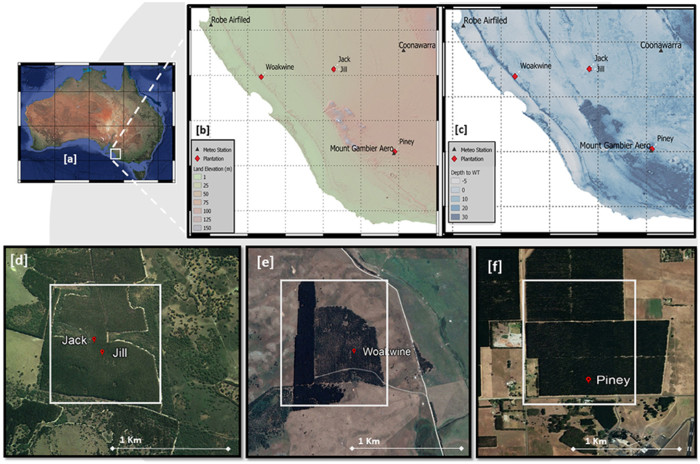
Figure 1. Location of the study area within Australia (a). Details of the topography, plantation sites, and meteorological stations used in this study (b). Details of the depth to WT of the upper unconfined aquifer (c). Satellite images of the four locations. Jack and Jill (d), Woakwine (e), and Piney (f). The squares represent the model cell and the CMRSET averaging area.

Softwood and hardwood forestry for timber production has been practiced in the area for more than a century. The dominant plantation timber species are Monterey Pine, Pinus radiata and Tasmanian Bluegum, Eucalyptus globulus (Benyon et al., 2006). Where these plantations overlie shallow WTs, which are within 6 m of the surface, it is likely that the trees directly access groundwater (Canadell et al., 1996; Benyon and Doody, 2004, 2015; Benyon et al., 2006, 2008).

Ecohydrological studies in the area have previously characterized vegetation, soil, climate, net irrigation, potential and actual evaporation, and depth to the WT, from silvicultural sites (Benyon et al., 2006). We selected four of these sites to answer the research questions. Two sites (“Woakwine” and “Jack”) had shallow WT depths (2.5 and 3m), Woakwine with a homogeneous soil profile and Jack a heterogeneous profile. One site (“Jill”) has a deep WT (10 m). The fourth site (“Piney”) records an average WT depth of 6 m (see Figure 1c for a map of the depth to WT). In general 6 m is the maximum WT depth at which the local forestry plantations can directly access groundwater (Benyon et al., 2006), thus this location is at the threshold between deep and shallow WT. Of these sites, Jill has a homogeneous soil profile, and Piney a heterogeneous profile. Climate is similar between the sites, and all contain mature trees: E. globulus except Piney, which contains P. radiata. Site details are presented in Table 1. Note that site names correspond to the those in Benyon et al. (2006), with the codenames in that paper being Woakwine: 4.EGl; Jack 5.EGl; Jill 6.EGl; and Piney 11.PR.

TABLE 1

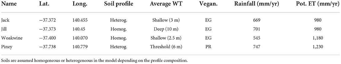
Table 1. Name, coordinates, and characteristics of the silviculture sites (Benyon et al., 2006).

2.2. Environmental data

2.2.1. Regional climatic data

The hydrogeological models used in this experiment are forced with rainfall and potential ET. Timeseries of each were obtained from three Bureau of Meteorology (BoM) stations (Figure 1b). Rainfall was obtained every 30 min, while potential ET values were daily totals. Rainfall data was aggregated, and potential ET disaggregated by dividing by 24, to produce hourly values used for modeling (Samain and Pauwels, 2013). When looking at water table dynamics at a regional scale, the simple ET disaggregation is considered appropriate enough, as long as consistency is kept between the model calibration and the application.

Simulations at Jack and Jill use climatic input from the Coonawarra station (Lat. −37.290, Long. 140.825 Station 026091), Piney uses data from the Mount Gambier Aero station (Lat. −37.747, Long. 140.773, Station 026021), and Woakwine from Robe Airfield station (Lat. −37.177, Long. 139.805 Station and 026105). Potential ET forcing inputs at Jack have a long gap between April and September 2002. As the gap affects some of the assimilation results, this period was omitted from the model evaluation.

2.2.2. Site characteristics

All site characteristics are presented in Benyon et al. (2006) (Table 1). Jack and Jill are paired sites, shown in Figure 1d and conceptually in Figure 2A. They are located only 110 m apart within the same E. globulus plantation. This plantation had a stem density of 1,175 stems ha⁻¹. Jack is located on a flat plain, over duplex soil (sand–clay) with depth to WT of ~ 3 m. Conversely, Jill is located at the crest of a sand dune, over a homogeneous sandy profile with the WT 10 m below the surface (Benyon et al., 2006).

FIGURE 2

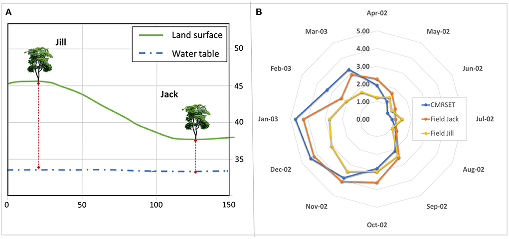
Figure 2. Conceptual representation of the local undulation affecting the depth to WT (A). Daily Actual ET from the CMRSET (averaged over 1 km²) and daily actual ET from field data at Jack and Jill (B).

Woakwine is an E. globulus plantation with a tree density of 818 stems ha⁻¹ (See Figure 1e). It grows on a homogeneous sandy soil with the WT at 3 m below the surface. Piney is a P. radiata plantation with a density of 1,200 stems ha⁻¹ (See Figure 1f). Piney grows on a duplex sandy-clay soil profile, with a WT depth of ~ 6 m, the threshold depth for plant transpiration from the groundwater (Benyon et al., 2006).

2.2.3. Water use

Climatically the sites experience different water deficits, defined as the difference between potential ET and rainfall (Table 1). This deficit is largest at Woakwine (635 mm year⁻¹), then Piney (483 mm year⁻¹), and smallest at Jack (311 mm year⁻¹) and Jill (279 mm year⁻¹). These deficits indicate the potential “demand” of the forestry plantations for groundwater use. When compared to actual ET estimates obtained through past lysimeter studies (Benyon and Doody, 2004; Benyon et al., 2006, 2008), however, the difference between precipitation and actual ET was clearly influenced by edaphic rather than climatic settings. For example, observed actual ET for Jack was 904 mm year⁻¹, which is larger than the 713 mm year⁻¹ for Jill (Benyon et al., 2006), suggesting that while potential ET—rainfall was comparable between the sites, some additional 235 mm year⁻¹ was transpired above rainfall at Jack (Data from in-situ pluviometers show an average difference of about 30 mm per year). The Jill site only relied on rainwater due to a much deeper depth the groundwater.

2.3. Remotely sensed ET

Remotely-sensed ET estimates were obtained from CMRSET (Guerschman et al., 2009). This data estimates actual ET based on surface reflectance from MODIS-Terra and interpolated climate data. It uses reflectance to rescale the Priestley-Taylor potential ET and calculates actual ET through the global vegetation moisture index (GVMI) and the enhanced vegetation index (EVI). Originally, the CMRSET algorithm was devised to produce monthly values of actual ET, using 16-day reflectance values, upscaled in time to a monthly value at 1 km resolution. In this version of the dataset, the CMRSET reached an averaged RMSE of 14.9 mm month⁻¹ when compared to five flux towers. A finer temporal and spatial resolution data-set, with a 250 m grid at a 8-day composite time step, is used in this study. Evapotranspiration values are rescaled to the model grid size (1 km²) as a result of averaging sixteen 250 × 250 m tiles.

The polar chart of Figure 2B shows, for Jack and Jill, the field-measured actual ET and the 1 km² averaged actual ET value from CMRSET. The spatial resolution of the resulting CMRSET dataset is well-suited to distinguish differences in actual ET between distant sites, but not the paired Jack and Jill sites as results are located within the same satellite observation grid. However, actual ET dynamics at the two sites differ. Jack has higher actual ET rates in summer, which are conceptually attributed to direct use of groundwater by vegetation, but not seen at Jill due to the deeper WT (Benyon et al., 2006). Jill, conversely, displays higher actual ET than Jack during May to August, presumably due to increased rainfall recorded at that site relative to Jack (Table 1). Given the differences in these two proximal sites, the simulations in this study can provide insight into how CMRSET resolution might impact the value of calibration to an assimilation of remotely sensed actual ET.

2.4. Models and simulations

2.4.1. Models

Water balance dynamics of the four sites were simulated using the UnSAT (Unsaturated zone & SATellite) model coupled to MODFLOW 2005, as described in Gelsinari et al. (2021). The UnSAT discretizes the soil column into a continuous series of vertical layers, applies the water balance to each layer, and solves for soil water content at each timestep. Forced by hourly climate data, UnSAT computes net-recharge, soil water content by depth [θ(z)], runoff, and actual ET. UnSAT is coupled to MODFLOW 2005 (Harbaugh, Arlen, 2005) through the net-recharge (i.e., gross recharge minus ET) term. This model configuration allows for plant water uptake from soil layers below the WT. As UnSAT is a conceptual model, its parameters are not necessarily entirely representative of the true soil physical conditions. Thus, parameters such as UnSAT saturated hydraulic conductivity (K_s) and MODFLOW saturated hydraulic conductivity (K_h) might differ. Untying K_s from K_h allows for a better representation of the different soil-hydraulic properties along the unsaturated zone.

While UnSAT runs at an hourly time step, MODFLOW applies an 8-day time step, aligned with MODIS observation frequency. MODFLOW computes the WT levels through space [WT(x,y)] which are then fed back to UnSAT, which recomputes the discretization of the unsaturated zone for the new local WT value. This non-iterative coupling scheme, similar to Zeng et al. (2019), provides a useful compromise between accuracy and computational burden of iterative schemes and has been validated in Gelsinari et al. (2020). This paper focuses on the use of actual ET data from remote sensing to inform these models.

2.4.2. Calibration, deterministic, and stochastic simulations

To address Research Questions 1 and 2, three different model calibration and simulations were executed:

- [Level 0]—Single Calibration. This is a simple, deterministic model calibration as routinely performed in groundwater models. The coupled UnSAT-MODFLOW model was calibrated using the Particle Swarm Optimization (PSO) algorithm (Kennedy and Eberhart, 1995; Shi and Eberhart, 1998) applied to modeled WT levels. For all locations, the WT level observations were split into a calibration period consisting of 40 8-day intervals, and a validation period consisting of the remainder of the observations. The PSO minimizes the Single Objective Function (SOF) defined as:

$\begin{array}{ll}\text{SOF}=\frac{\text{RMSE}(WT)}{\sigma (WT)},& (1)\end{array}$

where σ is standard deviation, and the Root Mean Square Error (RMSE) is defined as:

$\begin{array}{ll}\text{RMSE}=\sqrt{\frac{1}{L}{\displaystyle \sum _{k=1}^L}{(o_k-h_k)}^2},& (2)\end{array}$

where o_k and h_k are observed and modeled WT levels at time k, and L is the total number of observations. Calibrated parameters of the Level-0 simulations are listed in Table 2 under the SOF columns.

TABLE 2

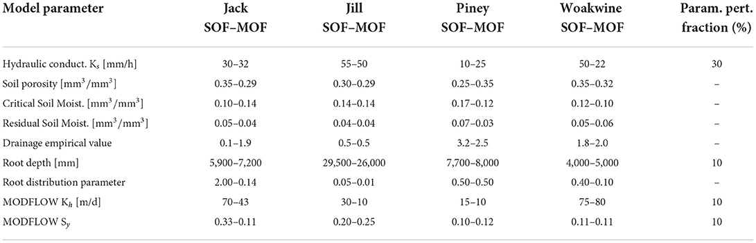
Table 2. Parameters and perturbation fractions used for the simulations.

- [Level 1]—Open Loop. This approach requires two steps, as informed by the results of using actual ET fluxes to improve model calibration (Gelsinari et al., 2021). First, the link between WT dynamic and actual ET fluxes needs to be established. This is achieved by minimizing a multi-objective function (MOF) defined by a combination of WT depth and actual ET as follows:

$\begin{array}{ll}\text{MOF}=\frac{\text{RMSE}(WT)}{\sigma (WT)}+\frac{\text{RMSE}(ET)}{\sigma (ET)},& (3)\end{array}$

Subsequently, the calibrated values were used as base for the generation of an ensemble of simulations to account for forcing inputs and parameter uncertainty.

To form this ensemble, all climatic inputs, initial conditions, and model parameters were treated as random samples. Climatic forcings were treated as the observed climate with additive noise sampled from a Gaussian distribution. Parameter values were treated as the deterministic MOF calibrated values, with multiplicative noise. The multiplier was varied between the parameters, as indicated by the “parameter perturbation fraction” (last column in Table 2). Initial conditions of WT levels were also perturbed with additive noise to induce a good spread in the ensemble from the early stages of the simulation. Calibrated parameters are listed in Table 2 under the MOF columns.

Care was taken during the ensemble generation to preserve the statistical accurateness while retaining the relationship between actual ET and WT levels obtained with the calibration (Pauwels and De Lannoy, 2009). By applying the verification skills described in Talagrand et al. (1997) (i.e., ensemble skill, ensemble spread, and mean square error), the mean of the ensemble was maintained statistically indistinguishable from the deterministic run used as its base. This would have made redundant the analysis of another (deterministic) level.

- [Level 2]—Data assimilation. These simulations use the Ensemble Kalman Filter (EnKF) to assimilate actual ET observations into the UnSAT model. The EnKF assimilation algorithm offers a reduced computational load and the capacity to deal with highly non-linear systems (Mitchell et al., 2002; Pauwels et al., 2013). The flexibility and low computational demand is achieved by propagating multiple, but limited, realizations of the model. This number defines the ensemble population. In this case, 32 ensemble members, generated through the process in Level 1, were used. This ensemble population is sufficient to represent the UnSAT-MODFLOW system in synthetic studies (Gelsinari et al., 2020) (see Supplementary Figure 2). Here we followed the approach adopted in Gelsinari et al. (2020, 2021). These studies provide a detailed description of the filter set-up and the interaction between the state variables, such as soil moisture and WT levels, and the assimilated quantity actual ET.

These simulation approaches are shown in Figure 3.

FIGURE 3

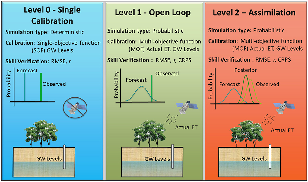
Figure 3. Simulation levels. In the probability inset: Forecast means the modeled actual ET. Observed means the satellite-based actual ET, which can be a single value, as in the case of Level-1, or a distribution, as required by the EnKF. Posterior means the distribution resulting from the filter update.

2.4.3. Simulation set-up

Simulations at the four sites were performed over different periods of time, according to the timing of data acquisition from previous field investigations, spanning from late 2000 to late 2007 (see Benyon et al., 2006). The domains consist horizontally of 5 × 1 cells (1 km² each), where the first and the last are constant head boundaries, and vertically of one convertible layer for the saturated zone simulating the unconfined aquifer. This simple groundwater model conceptualization aims to model WT levels and actual ET flux at a single cell per simulation. Model set up was shown to adequately represent the system through a sensitivity analysis of different domain sizes, as described in Gelsinari et al. (2021), and in Supplementary Figure 1.

2.5. Simulation skill verification

Simulation results were evaluated using several different metrics. These included: (i) RMSE (see Equation 2), (ii) the Pearson correlation coefficient (r) as in Pearson (1920), and (iii) the Continuous Ranked Probability Score (CRPS—Hersbach, 2000), a measure of the difference between the predicted and observed cumulative distributions. CRPS avoids some of the limitations of sum of squared error metrics (like RMSE or r) which can be highly sensitive to the largest errors, potentially biasing the model skill evaluation (Schneider et al., 2020).

The CRPS for the probability density function P(x) given by the ensemble simulation for the variable of interest x (i.e., ET and WT levels) and calculated at a specific timestep k is defined by:

$\begin{array}{ll}CRP{S}_k={\displaystyle {\int }_{+\infty }^{-\infty }{(P{(x)}_k-P_o{(x)}_k)}^{2}dx,}& (4)\end{array}$

where P_o is distribution of observations. As the observation at a given time is usually a single value, P_o(x) is equivalent to H(x−x_a), where H is the Heaviside function (Bracewell, 2000), applied similarly to Gelsinari et al. (2021).

With this definition, the CRPS is interpreted as the area between the cumulative probability function of the ensemble forecast and the observation function (linear). A CRPS of zero implies a perfect deterministic forecast (Hersbach, 2000). The CRPS varies from 0 to 1, and is usually calculated for all timesteps and then averaged over a simulation period.

RMSE values were calculated for all three calibration strategies used in these experiments. When the simulations were based on a parameter ensemble, RMSE values were calculated for the ensemble average predictions. CRPS values were calculated for the ensemble simulations only (i.e., the open loop and data assimilation simulations), following Equation (4). Verification skills were calculated over a validation period as previously described in Section 2.4.2.

Residuals of actual ET were computed as:

$\begin{array}{ll}RET={\displaystyle \sum _{k=1}^L}(i_k-j_k),& (5)\end{array}$

where i_k is the satellite observed actual ET and j_k is the modeled actual ET at time k, and L is the total number of observations. Values greater than zero indicate that the modeled actual ET under-estimates observations, while values higher than zero imply that the modeled actual ET is lower than the remote sensing actual ET observations.

3. Results

Performance of the simulations based on the RMSE and r are presented in Table 2 for both actual ET and for WT levels. The ensembles were generated so that the mean of the Level-1 ensemble is statistically equivalent to the deterministic simulation. RMSE and r-values calculated over the means (for Level-1 and Level-2) and compared to those of the deterministic (Level-0) simulation provide an assessment of the simulation performance against Level-0 as a benchmark.

The CRPS values (Table 4) provide an additional assessment of the ensemble performances for the two stochastic modeling approaches. Specifically, comparing CRPS between Level-2 and Level-1 quantifies the benefits to model performance of assimilating ET data through the EnKF versus calibrating to ET. The results are discussed separately for the model predictions of actual ET and WT.

3.1. Evapotranspiration

Including actual ET in the models through calibration or assimilation improved simulations of actual ET in the sense that RMSEs declined and r increased, for every site other than Jill. The improvements were most evident at Jack, in which the RMSE decreased by ~30% and the r improved by ~100% upon inclusion of actual ET data in the modeling. Improvements at Woakwine and Piney are more modest, but still represent ~20% reductions in RMSE (see Table 3). The modeled actual ET at Jack is shown in the top panel of Figure 4. This panel shows that the Level-0 modeled actual ET (yellow line) greatly underestimates MODIS-CMRSET observations, an underestimation which is overcome by incorporating actual ET information, in the Level-1 and Level-2 models. The cause of the peak in ET of April 2003 is due to the model input, as this is similarly found at all the three levels, meaning that is not an artifact of the Ensemble Kalman filter update or the input perturbation strategy. The model response has been interpreted as a situation where the soil profile is particularly wet combined with high Potential ET (similar to summer conditions), causing the model to over-estimate actual ET.

TABLE 3

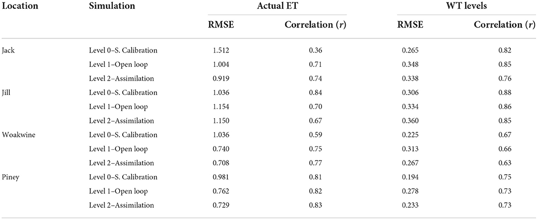
Table 3. RMSE and r calculated on actual ET and WT levels.

FIGURE 4

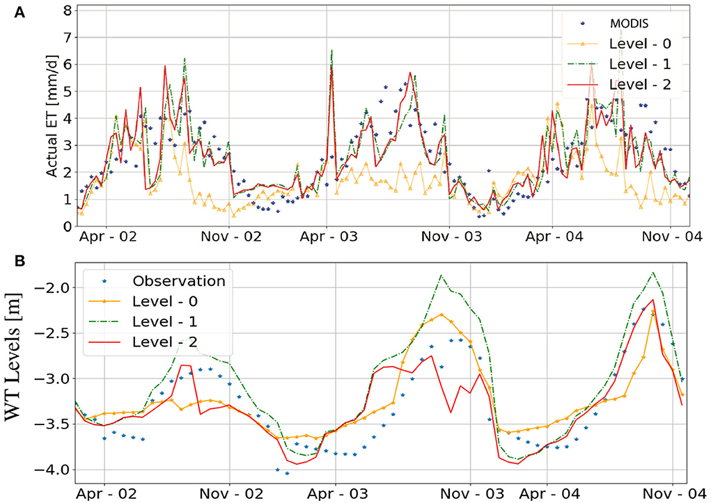
Figure 4. Remotely sensed (MODIS) and modeled actual ET (Level-0 to Level-1) (A). Observed and modeled WT levels (B) at the Jack field site.

As described in Section 2.4.3, the deep WT at Jill occurs within the same MODIS-CMRSET pixel as the shallow WT at Jack, but represents a very different water availability scenario for the plantation. With the model for Jack reproducing actual ET fluxes well when constrained with MODIS-CMRSET observations, it is perhaps unsurprising that the opposite occurs in the different environment at Jill. Level-1 and Level-2 models at Jill had an ~10% higher RMSE and an ~15% lower r relative to the Level-0 model.

CRPS values, aggregated over the validation period for the model runs, are reported in Table 4, with the ET results shown on the left hand side. CRPS values calculated at each time represent the actual ET level distribution of the ensemble around the observation, with a low value indicating good agreement and thus reduced uncertainty. The CRPS suggest that assimilation improves the ET ensemble distributions at Jack, Woakwine, and Piney, although the improvements are relatively small in percentage terms, and marginal at Jack. At Jill, however, the assimilation of actual ET increases the CRPS, actually worsening the model performance relative to calibration.

TABLE 4

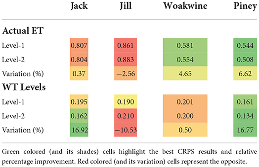
Table 4. CRPS values for the two stochastic simulation levels and relative percentage variation of Level–2 over Level–1.

Figure 5 shows the residuals of 6-month aggregated values of actual ET for the single calibration, open-loop and assimilation runs, compared to CMRSET predictions. Values above zero indicate overestimation of modeled ET compared to remotely sensed observations (CMRSET), while values below zero are underestimates (Figure 5). For almost all runs across sites and years, the groundwater models calibrated only to WT levels underestimate actual ET. The right side of Figure 5 shows the average of these residuals for each 6 month period, showing that Level-0 models underestimate actual ET by between 74 and 140 mm year⁻¹. However, these underestimates were reduced at Level-2 by 25 % (at Jill) to 70 % (i.e., Jack and Piney). Examination of the calibrated parameters of the Level-0 models show that they predict shorter root lengths and a more linear root density distribution than do the Level-1 and Level-2 simulations.

FIGURE 5

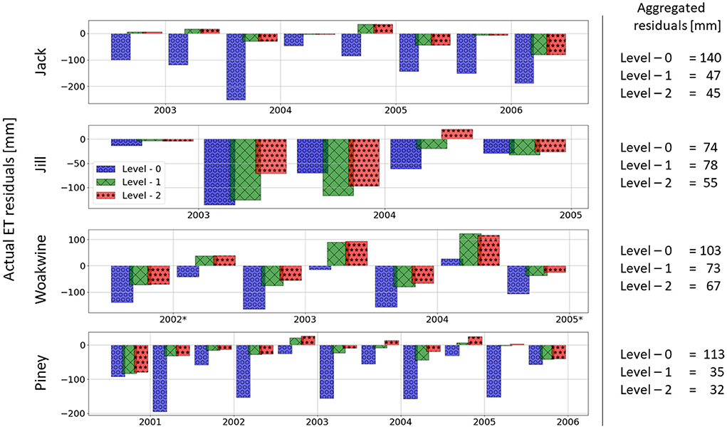
Figure 5. Residuals of the actual ET (RET) depths calculated as 6-month aggregates, and aggregated RET over the simulation periods.

3.2. WT Levels

The Level-0 simulations generated the best performance in terms of WT predictions as measured by RMSE in all the locations, as shown in Table 3, with the r being similar for most of the simulations. The CRPS metrics in Table 4, however, show that assimilation can improve ensemble WT predictions compared to the open loop, notably at Piney and Jack, in which quite large percentage improvements in CRPS are achieved by assimilation. The r in the Level-2 Jack simulation is reduced; this is a consequence of the EnKF continuously updating the WT level (see Figure 4B). For example, the Level-2 model shows abrupt changes in WT in the period of June–December 2003. These changes are due to the filter causing rapid and non-smooth changes in WT predictions, which lower performance metrics. Not all abrupt changes in the model predictions, however, are associated with the EnKF. For example, the shifts in WT around September 2002 occur in both Level-1 and Level-2 simulations, and are associated with the gap of the potential ET forcing data. As a results of this gap, the period from 2002/04/01 to 2002/10/31 was removed when calculating performance metrics.

Similarly to Jack, the CRPS for Piney improves between Level-1 and Level-2 and the performance of the model is good overall. However, the r-value is not improved. At Jill and Woakwine, CRPS, RMSE, and r worsened or were close to unchanged between Level-1 and Level-2. At Jill, the declining performance may indicate that actual ET data were disinformative of the local water balance (Beven and Westerberg, 2011).

4. Discussion

Including actual ET in the simulations via calibration or assimilation improved the ability of the models to represent ET fluxes at all sites except Jill, generally at the expense of the ability of the models to represent WT dynamics. Overall, assimilation of actual ET timeseries improved the representation of ET fluxes and the ensemble predictions of WT levels, while slightly worsening the RMSE and values of WT predictions compared to the deterministic run.

4.1. How do site attributes affect modeling strategies?

Across both actual ET and WT, and for all levels modeled, the model predictions were most reliable at Piney. This site exhibited the highest stem density of all the plantations, which is likely to have produced near homogeneous conditions of water use, and may mean that satellite observations of actual ET were more reliable than when made over the more variable land surface conditions at the other sites.

The benefits of informing model calibration with actual ET were greatest at the Jack, Piney, and Woakwine sites. These sites had relatively shallow WT that were at the limit of or within the rooting depth of the plantations, suggesting that WT levels might be well coupled to evaporation at these locations. Actual ET assimilation has previously been shown to perform well in areas with significant groundwater-vegetation interactions (Gelsinari et al., 2020).

Information provided from actual ET, reduced model performance only at the Jill site. Presumably this is due to the localized deep WT at Jill, which is not representative of the conditions across the MODIS-CMRSET pixels used for the analysis. Under such a condition, the ET data is disinformative rather than informative, and worsens the model predictions. There is less differentiation between calibration and assimilation under these circumstances, because the ET in all cases does not add a meaningful constraint to the groundwater model. Preliminary analyses of digital elevation models could be useful to identify such locations that might exist in one remote sensing pixel.

4.2. Recommendations

Across all sites, incorporating actual ET information into model parameterization reduced the quality of predictions of the WT dynamics while improving the prediction of ET fluxes. This suggests that an improvement in the fidelity of modeling the local water balance might require reduced accuracy in modeling the specific signature of WT levels. It also indicates the risks inherent with using only a single metric to evaluate a model performance: overfitted models based on a single measurement can overestimate a model's ability to replicate all hydrological processes. If the models are only evaluated against WT level results, the single calibration (e.g., WT levels) seems to produce good results.

However, the quantitative management of groundwater resources requires having good estimates of fluxes, such as recharge and ET, and not only of groundwater levels. If the volume of water transpired by plantations is underestimated in models (as it was in all Level-0 models) then management based on model interpretations could be incorrect. Underestimation of water used by forest plantations could contribute to unsustainable management of groundwater resources, which itself can trigger non-linear and hard-to-reverse changes in water resource availability. By accounting for satellite based remote sensing ET, the models better replicated the fluxes of plant transpiration, especially in areas where plant-groundwater interactions were strong. The benefits of informing the model with actual ET greatly improved the estimates of ET volumes, at the cost of losing some precision in the estimates of WT levels. However, this loss of precision is not problematic with the benefit of obtaining better estimates of important hydrologic quantities such as ET or recharge.

Consequently, using actual ET observations from satellites is a valuable approach to improving the fidelity of groundwater models, especially if remote sensing outputs can be bias corrected using field collected data. This approach may be particularly beneficial in sites exhibiting vegetation-groundwater interactions, which closely couple WT levels to ET.

The difference between Level-1 and Level-2 is more subtle than the improvements relative to Level-0 models. There is a substantial increase in effort and skill needed to set up an EnKF scheme, and the benefit of doing so requires careful evaluation. In densely vegetated areas where the WT is within the reach of the plant roots, such as Jack, Woakwine and Piney, data assimilation improved RMSE and CRPS values for WT, actual ET and thus volumes of transpired water. Overall, however, the improvements in simulations between simple calibration and assimilation were relatively modest, and data assimilation may not be necessary for successful use of ET in groundwater models in general.

Although one of the key advantages of remote sensing data is to provide spatially distributed data, in this experiment that piece of information was not used as the focus was on the calibration and data assimilation of models using actual ET data. Regardless of the calibration method, the potential for rapid spatial changes in depth to groundwater and water balance within a satellite pixel is the main constraint on using ET for model calibration. Modelers should determine whether local groundwater dynamics can be reasonably represented at the scale of the satellite ET pixel before proceeding.

Future work in model evaluation could consider longer time periods, more sites, the use of drones for the estimation of actual ET at much higher spatial resolutions (Marzahn et al., 2020), and further refining metrics. For example, representing the CRPS as a time dependent metric allows for more in-depth analyses to identify the specific conditions for which an ensemble is or is not improved (Gelsinari et al., 2021). Similarly, it could further explore the role of the soil profile in moderating model performance. During this experiment, identifying and isolating the effects of integrating ET data over different soil profiles (i.e., Homogeneous vs. Heterogenous) was not conclusive. With the results obtained at Piney and Jack, it was shown that heterogenous profiles (usually considered more difficult to model and calibrate) do not represent an obstacle per se to the application of this methodology.

Here, we focused on measured actual ET fluxes and WT levels, and were not able to examine how ET information altered prediction of the distribution of soil moisture in the profile. A specific assessment of the soil moisture content at all the locations could provide more insights into the effect of using actual ET retrievals on model fidelity in the unsaturated zone. In this study, water content distributions accounted for by using ET fluxes as a proxy for the water content along the soil column.

5. Conclusion

This study focused on the ability of a satellite-based ET dataset (CMRSET) to inform coupled unsaturated zone-groundwater models. Three levels of application of the remotely sensed ET were applied to four plantations in the water-limited, south-east of South Australia. These plantations show a combination of WT depth, soil profiles, and vegetation type for each of the locations that is representative of numerous other plantations in the area. Thus, they provide insights into the value of using satellite based actual ET to improve modeled hydrological quantities.

The findings of this paper show that incorporating actual ET fluxes when modeling vegetated areas substantially improved the model capability of accounting for water fluxes. This is especially evident in areas where vegetation has direct access to groundwater, resulting in higher transpiration. For these areas the error reduction in predicted ET volumes is up to an order of magnitude.

Stochastic simulations of a model calibrated using WT level and actual ET data were performed to account for forcing input and parameter uncertainties. For actual ET, Level-1 RMSE and r-values report improvements of up to 50% for all the locations, with the exception of deep WT levels (i.e., Jill), when compared to the model calibrated using only WT level data. The deterministic simulations (Level-0) calibrated on WT levels only performed better than the stochastic when evaluated against WT levels. This comes at the price of poorer performances when simulating actual ET, which is a variable of great importance in water limited environments.

The application of ET assimilation (i.e., Level-2) to these locations is evaluated through the RMSE and the CRPS. The data assimilated simulations present reduced actual ET and WT levels RMSE compared to calibrating with a MOF, and also improves the ensemble distribution as indicated by CRPS values. However, the value of performing a complex ET assimilation is not always justified by the magnitude of the error reduction. Improvements were more obvious in densely vegetated areas when plants have access to groundwater. Conversely, where groundwater was deep and vegetation water use was lower, a reduced filter effect was shown, which is in agreement with the lack of direct correlation between actual ET and WT when the latter is deep. Finally, these results indicate that benefits can be obtained by using actual ET observation in the calibration phase, as performed through the MOF.

These findings support the use of actual ET to inform hydrogeological models as a valuable tool for the quantitative management of groundwater resources, and is particularly relevant in silvicultural areas. Updating the model with readily available, continuous, satellite-based ET time-series helps in improving assessments of water consumption by forest plantations accessing groundwater in water-limited environments. More accurate estimates of water used by vegetation is beneficial for water resource managers who are more often dealing with problems arising from unaccounted water use in already heavily allocated groundwater systems. The method has the potential to provide useful information for non stationary systems, such as environments experiencing climate change related stresses.

Data availability statement

The datasets presented in this study can be found in online repositories. The names of the repository/repositories and accession number(s) can be found at: https://doi.org/10.6084/m9.figshare.21211130.

Author contributions

SG, RD, ED, and VP contributed to conception and design of the study. SG organized the database, performed the statistical analysis, and wrote the first draft of the manuscript. TD and ST helped in the interpretation of the results and the structuring of the manuscript. All authors contributed to manuscript revision. All authors contributed to the article and approved the submitted version.

Funding

Funding for this project has been provided by the CSIRO Land and Water Effective Floodplain Management Project. Funding for these plantation sites was provided by CSIRO, the South Australian Department of Water, Land, and Biodiversity Conservation, the South East Catchment Water Management Board, Auspine, Green Triangle Forest Products, the Forest and Wood Products Research and Development Corporation, the Green Triangle Regional Plantation Committee, and the District Council of Grant.

Acknowledgments

We wish to gratefully acknowledge Dr. Richard Benyon who led the research collecting the data for the sites presented.

Conflict of interest

The authors declare that the research was conducted in the absence of any commercial or financial relationships that could be construed as a potential conflict of interest.

Publisher's note

All claims expressed in this article are solely those of the authors and do not necessarily represent those of their affiliated organizations, or those of the publisher, the editors and the reviewers. Any product that may be evaluated in this article, or claim that may be made by its manufacturer, is not guaranteed or endorsed by the publisher.

Supplementary material

The Supplementary Material for this article can be found online at: https://www.frontiersin.org/articles/10.3389/frwa.2022.932641/full#supplementary-material

References

Banks, E. W., Brunner, P., and Simmons, C. T. (2011). Vegetation controls on variably saturated processes between surface water and groundwater and their impact on the state of connection. Water Resour. Res. 47, 1–14. doi: 10.1029/2011WR010544

CrossRef Full Text | Google Scholar

Benyon, R. G., and Doody, T. M. (2004). Water Use by Tree Plantations in South East South Australia. Technical report, CSIRO Forestry and Forest Products.

Google Scholar

Benyon, R. G., and Doody, T. M. (2015). Comparison of interception, forest floor evaporation and transpiration in Pinus radiata and Eucalyptus globulus plantations. Hydrol. Process. 29, 1173–1187. doi: 10.1002/hyp.10237

CrossRef Full Text | Google Scholar

Benyon, R. G., Doody, T. M., Theiveyanathan, S., and Koul, V. (2008). Plantation Forest Water Use in Southwest Victoria. Technical report, CSIRO: Water for a Healthy Country National Research Flagship.

Google Scholar

Benyon, R. G., Theiveyanathan, S., and Doody, T. M. (2006). Impacts of tree plantations on groundwater in south-eastern Australia. Aust. J. Bot. 54:181. doi: 10.1071/BT05046

CrossRef Full Text | Google Scholar

Beven, K. (2006). A manifesto for the equifinality thesis. J. Hydrol. 320, 18–36. doi: 10.1016/j.jhydrol.2005.07.007

CrossRef Full Text | Google Scholar

Beven, K., and Westerberg, I. (2011). On red herrings and real herrings: disinformation and information in hydrological inference. Hydrol. Process. 25, 1676–1680. doi: 10.1002/hyp.7963

CrossRef Full Text | Google Scholar

Bracewell, R. (2000). Heaviside's Unit Step Function, H(x). The Fourier Transform and Its Applications, 3rd Edn. New York, NY: McGraw-Hill.

Google Scholar

Canadell, J., Jackson, R. B., Ehleringer, J. B., Mooney, H. A., Sala, O. E., and Schulze, E. D. (1996). Maximum rooting depth of vegetation types at the global scale. Oecologia 108, 583–595. doi: 10.1007/BF00329030

PubMed Abstract | CrossRef Full Text | Google Scholar

Doble, R. C., and Crosbie, R. S. (2017). Review: Current and emerging methods for catchment-scale modelling of recharge and evapotranspiration from shallow groundwater. Hydrogeol. J. 25, 3–23. doi: 10.1007/s10040-016-1470-3

CrossRef Full Text | Google Scholar

Doble, R. C., Pickett, T., Crosbie, R. S., Morgan, L. K., Turnadge, C., and Davies, P. J. (2017). Emulation of recharge and evapotranspiration processes in shallow groundwater systems. J. Hydrol. 555, 894–908. doi: 10.1016/j.jhydrol.2017.10.065

CrossRef Full Text | Google Scholar

Dresel, P. E., Dean, J. F., Perveen, F., Webb, J. A., Hekmeijer, P., Adelana, S. M., et al. (2018). Effect of eucalyptus plantations, geology, and precipitation variability on water resources in upland intermittent catchments. J. Hydrol. 564, 723–739. doi: 10.1016/j.jhydrol.2018.07.019

CrossRef Full Text | Google Scholar

Dye, P., and Versfeld, D. (2007). Managing the hydrological impacts of South African plantation forests: an overview. For. Ecol. Manage. 251, 121–128. doi: 10.1016/j.foreco.2007.06.013

CrossRef Full Text | Google Scholar

Famiglietti, J. S., and Rodell, M. (2013). Water in the balance. Science 340, 1300–1301. doi: 10.1126/science.1236460

PubMed Abstract | CrossRef Full Text | Google Scholar

Farrington, P., and Bartle, G. (1991). Recharge beneath a Banksia woodland and a Pinus pinaster plantation on coastal deep sands in south Western Australia. For. Ecol. Manage. 40, 101–118. doi: 10.1016/0378-1127(91)90096-E

CrossRef Full Text | Google Scholar

Gelsinari, S., Doble, R., Daly, E., and Pauwels, V. (2020). Feasibility of improving groundwater modeling by assimilating evapotranspiration rates. Water Resour. Res. 56:e2019WR025983. doi: 10.1029/2019WR025983

CrossRef Full Text | Google Scholar

Gelsinari, S., Pauwels, V. R., Daly, E., Van Dam, J., Uijlenhoet, R., Fewster-Young, N., et al. (2021). Unsaturated zone model complexity for the assimilation of evapotranspiration rates in groundwater modelling. Hydrol. Earth Syst. Sci. 25, 2261–2277. doi: 10.5194/hess-25-2261-2021

CrossRef Full Text | Google Scholar

Glenn, E. P., Doody, T. M., Guerschman, J. P., Huete, A. R., King, E. A., McVicar, T. R., et al. (2011). Actual evapotranspiration estimation by ground and remote sensing methods: the Australian experience. Hydrol. Process. 25, 4103–4116. doi: 10.1002/hyp.8391

CrossRef Full Text | Google Scholar

Green, T. R., Taniguchi, M., Kooi, H., Gurdak, J. J., Allen, D. M., Hiscock, K. M., et al. (2011). Beneath the surface of global change: Impacts of climate change on groundwater. J. Hydrol. 405, 532–560. doi: 10.1016/j.jhydrol.2011.05.002

CrossRef Full Text | Google Scholar

Greenwood, A. J. (2013). The first stages of Australian forest water regulation: national reform and regional implementation. Environ. Sci. Policy 29, 124–136. doi: 10.1016/j.envsci.2013.01.012

CrossRef Full Text | Google Scholar

Greenwood, A. J., Benyon, R. G., and Lane, P. N. (2011). A method for assessing the hydrological impact of afforestation using regional mean annual data and empirical rainfall-runoff curves. J. Hydrol. 411, 49–65. doi: 10.1016/j.jhydrol.2011.09.033

CrossRef Full Text | Google Scholar

Guerschman, J. P., McVicar, T. R., Vleeshower, J., Van Niel, T. G., Pen̄a-Arancibia, J. L., and Chen, Y. (2022). Estimating actual evapotranspiration at field-to-continent scales by calibrating the CMRSET algorithm with MODIS, VIIRS, Landsat and sentinel-2 data. J. Hydrol. 605:127318. doi: 10.1016/j.jhydrol.2021.127318

CrossRef Full Text | Google Scholar

Guerschman, J. P., van Dijk, A., Mattersdorf, G., Beringer, J., Hutley, L. B., Leuning, R., et al. (2009). Scaling of potential evapotranspiration with MODIS data reproduces flux observations and catchment water balance observations across Australia. J. Hydrol. 369, 107–119. doi: 10.1016/j.jhydrol.2009.02.013

CrossRef Full Text | Google Scholar

Harbaugh, A. W. (2005). MODFLOW-2005: The U.S. Geological Survey Modular Ground-Water Model the Ground-Water Flow Process. U.S. Geol. Surv. Tech. Methods, 253. doi: 10.3133/tm6A16

CrossRef Full Text | Google Scholar

Hersbach, H. (2000). Decomposition of the continuous ranked probability score for ensemble prediction systems. Weather Forecast. 15, 559–570. doi: 10.1175/1520-0434(2000)015&lt;0559:DOTCRP&gt;2.0.CO;2

CrossRef Full Text | Google Scholar

Immerzeel, W., and Droogers, P. (2008). Calibration of a distributed hydrological model based on satellite evapotranspiration. J. Hydrol. 349, 411–424. doi: 10.1016/j.jhydrol.2007.11.017

CrossRef Full Text | Google Scholar

Kalma, J., McVicar, T., and McCabe, M. (2008). Estimating land surface evaporation: a review of methods using remotely sensed surface temperature data. Surveys Geophys. 29, 421–469. doi: 10.1007/s10712-008-9037-z

CrossRef Full Text | Google Scholar

Kennedy, J., and Eberhart, R. (1995). “Particle swarm optimization,” in Proceedings 1995 of IEEE International Conference on Neural Networks, Vol. 4 (Perth, WA), 1942–1948.

Google Scholar

Leblanc, M., Tweed, S., van Dijk, A., and Timbal, B. (2012). A review of historic and future hydrological changes in the Murray-Darling Basin. Glob. Planet. Change 80–81, 226–246. doi: 10.1016/j.gloplacha.2011.10.012

CrossRef Full Text | Google Scholar

Lopes, J. D., Rodrigues, L. N., Imbuzeiro, H. M. A., and Pruski, F. F. (2019). Performance of SSEBOP model for estimating wheat actual evapotranspiration in the Brazilian savannah region. International Journal of Remote Sensing 40, 6930–6947. doi: 10.1080/01431161.2019.1597304

CrossRef Full Text | Google Scholar

Marzahn, P., Flade, L., and Sanchez-Azofeifa, A. (2020). Spatial estimation of the latent heat flux in a tropical dry forest by using unmanned aerial vehicles. Forests 11, 1–16. doi: 10.3390/f11060604

CrossRef Full Text | Google Scholar

McVicar, T., Vleeshouwer, J., Van Niel, T., and Guerschman, J. (2022). Actual Evapotranspiration for Australia using CMRSET algorithm. Terrestrial Ecosystem Research Network. (Dataset). doi: 10.25901/gg27-ck96

PubMed Abstract | CrossRef Full Text | Google Scholar

Mitchell, H. L., Houtekamer, P. L., and Pellerin, G. (2002). Ensemble size, balance, and model-error representation in an ensemble Kalman filter*. Mon. Weather Rev. 130, 2791–2808. doi: 10.1175/1520-0493(2002)130&lt;2791:ESBAME&gt;2.0.CO;2

CrossRef Full Text | Google Scholar

Moore, C., and Doherty, J. (2006). The cost of uniqueness in groundwater model calibration. Adv. Water Resour. 29, 605–623. doi: 10.1016/j.advwatres.2005.07.003

CrossRef Full Text | Google Scholar

Novick, K., Biederman, J., Desai, A., Litvak, M., Moore, D., Scott, R., et al. (2018). The ameriflux network: a coalition of the willing. Agric. For. Meteorol. 249, 444–456. doi: 10.1016/j.agrformet.2017.10.009

CrossRef Full Text | Google Scholar

Pauwels, V. R. N., and De Lannoy, G. J. M. (2009). Ensemble-based assimilation of discharge into rainfall-runoff models: a comparison of approaches to mapping observational information to state space. Water Resour. Res. 48:W08428. doi: 10.1029/2008WR007590

CrossRef Full Text | Google Scholar

Pauwels, V. R. N., De Lannoy, G. J. M., Hendricks Franssen, H.-J., and Vereecken, H. (2013). Simultaneous estimation of model state variables and observation and forecast biases using a two-stage hybrid Kalman filter. Hydrol. Earth Syst. Sci. 17, 3499–3521. doi: 10.5194/hess-17-3499-2013

CrossRef Full Text | Google Scholar

Pearson, K. (1920). Notes on the history of correlation. Biometrika 13, 25–45. doi: 10.1093/biomet/13.1.25

CrossRef Full Text | Google Scholar

Samain, B., and Pauwels, V. R. N. (2013). Impact of potential and (scintillometer-based) actual evapotranspiration estimates on the performance of a lumped rainfall-runoff model. Hydrol. Earth Syst. Sci. 17, 4525–4540. doi: 10.5194/hess-17-4525-2013

CrossRef Full Text | Google Scholar

Schneider, R., Henriksen, H. J., and Stisen, S. (2020). A robust objective function for calibration of groundwater models in light of deficiencies of model structure and observations. Hydrol. Earth Syst. Sci. Discuss. 1–26. doi: 10.5194/hess-2019-685

CrossRef Full Text | Google Scholar

Shi, Y., and Eberhart, R. (1998). “A modified particle swarm optimizer,” in 1998 IEEE International Conference on Evolutionary Computation. Proceedings IEEE World Congress on Computational Intelligence (Cat. No.98TH8360), 69–73. doi: 10.1109/ICEC.1998.699146

PubMed Abstract | CrossRef Full Text | Google Scholar

Silberstein, R. P., Dawes, W. R., Bastow, T. P., Byrne, J., and Smart, N. F. (2013). Evaluation of changes in post-fire recharge under native woodland using hydrological measurements, modelling and remote sensing. J. Hydrol. 489, 1–15. doi: 10.1016/j.jhydrol.2013.01.037

CrossRef Full Text | Google Scholar

Swaffer, B. A., Habner, N. L., Holland, K. L., and Crosbie, R. S. (2020). Applying satellite-derived evapotranspiration rates to estimate the impact of vegetation on regional groundwater flux. Ecohydrology 13, 1–14. doi: 10.1002/eco.2172

CrossRef Full Text | Google Scholar

Talagrand, O., Vautard, R., and Strauss, B. (1997). Evaluation of Probabilistic Prediction Systems. Technical report, Meteo-France, Illkirch.

Google Scholar

van Der Salm, C., Denier Van Der Gon, H., Wieggers, R., Bleeker, A., and van Den Toorn, A. (2006). The effect of afforestation on water recharge and nitrogen leaching in The Netherlands. For. Ecol. Manage. 221, 170–182. doi: 10.1016/j.foreco.2005.09.027

CrossRef Full Text | Google Scholar

Walker, G. R., Crosbie, R. S., Chiew, F. H. S., Peeters, L., and Evans, R. (2021). Groundwater impacts and management under a drying climate in southern Australia. Water 13:3588. doi: 10.3390/w13243588

CrossRef Full Text | Google Scholar

Zeng, J., Yang, J., Zha, Y., and Shi, L. (2019). Capturing soil-water and groundwater interactions with an iterative feedback coupling scheme : new HYDRUS package for MODFLOW. Hydrol. Earth Syst. Sci. 23, 637–655. doi: 10.5194/hess-23-637-2019

CrossRef Full Text | Google Scholar