Adaptation of water resources management under climate change

The rapid growth of demand in agricultural production has created water scarcity issues worldwide. Simultaneously, climate change scenarios have projected that more frequent and severe droughts are likely to occur. Adaptive water resources management has been suggested as one strategy to better coordinate surface water and groundwater resources (i.e., conjunctive water use) to address droughts. In this study, we enhanced an aggregated water resource management tool that represents integrated agriculture, water, energy, and social systems. We applied this tool to the Yakima River Basin (YRB) in Washington State, USA. We selected four indicators of system resilience and sustainability to evaluate four adaptation methods associated with adoption behaviors in alleviating drought impacts on agriculture under RCP4.5 and RCP 8.5 climate change scenarios. We analyzed the characteristics of four adaptation methods, including greenhouses, crop planting time, irrigation technology, and managed aquifer recharge as well as alternating supply and demand dynamics to overcome drought impact. The results show that climate conditions with severe and consecutive droughts require more financial and natural resources to achieve well-implemented adaptation strategies. For long-term impact analysis, managed aquifer recharge appeared to be a cost-effective and easy-to-adopt option, whereas water entitlements are likely to get exhausted during multiple consecutive drought events. Greenhouses and water-efficient technologies are more effective in improving irrigation reliability under RCP 8.5 when widely adopted. However, implementing all adaptation methods together is the only way to alleviate most of the drought impacts projected in the future. The water resources management tool helps stakeholders and researchers gain insights in the roles of modern inventions in agricultural water cycle dynamics in the context of interactive multi-sector systems.

Introduction

Water resource management at the Food-Energy-Water (FEW) nexus is increasingly being investigated and scrutinized for synergies and conflicts (Lele et al., 2013; Abbott et al., 2017; Kaddoura and El Khatib, 2017). The improvement of water provisioning for agricultural producers is of utmost importance because they are continually being challenged by the increasing frequencies of extreme weather, such as periods of drought, especially under future climate projections (Hatfield et al., 2011; National Research Council, 2011; Wang et al., 2011; Church et al., 2018). For example, across the Cascades to the eastern valleys in the Pacific Northwest (PNW), farmers encounter water scarcity issues frequently as a result of insufficient water supply and large demands from agricultural activities (Chang et al., 2013). Adaptation is needed to achieve reliability, resilience, and sustainability of water resource systems in agriculture (Rickards and Howden, 2012; Iglesias and Garrote, 2015; Nam et al., 2015).

Water resource systems can become more reliable by improving water supply or reducing water demand. Increasing water storage is a key strategy to create a buffer between seasonally available precipitation, snowmelt, and water needs during the agricultural growing season. Reservoirs, ponds, natural water bodies, and aquifers are examples of available water storage. Recently, managed aquifer recharge (MAR) has received more attention as a method by which extra water is stored in the aquifer through infiltration or well-injection, instead of releasing water downstream (Dillon et al., 2010). California and Arizona have been developing MAR to address droughts as early as the 1960s with outstanding outcomes in enhancing drought resilience (Scanlon et al., 2016). In Europe, the history of MAR started as early as 1810 in the UK, and it has been playing an important role in water supply in many European countries for over a century (Sprenger et al., 2017). However, MAR is not yet widely implemented in agriculturally intensive regions such as the Yakima River Basin in the PNW (Zhao et al., 2021). Vano et al. (2010) found that farmers have suffered from water shortfalls 14% of years, on average, from 1917 to 2006. Their study shows that the frequency is projected to increase to 68% by the 2080s under climate change scenarios (i.e., A1B scenario: balance across all energy sources) if no actions are taken.

Agricultural water demand, among other water demand sectors, takes up about 65% of the total water withdrawals, and 90% of global total water consumption comes from agriculture (Oki and Kanae, 2006). Irrigation water demand and consumption are greatly affected by crop type, weather condition, and irrigation system efficiency. Adaptive management that increases capacity and efficiency for irrigation and coordinates land use and land cover change can potentially ease the projected water stress. Technology advances in irrigation systems are often focused on improving crop yield and thereby increasing consumptive water use (Ward and Pulido-Velazquez, 2008; Bjornlund et al., 2009), which may lead to decreased return flow. Adoption of water conservation technologies in irrigation, such as drip or sprinkler systems, has been encouraged due to prospective economic returns (Marques et al., 2005) as well as to reduce evaporation losses and reduce water demand. Greenhouses (GHs) equipped with efficient water application technology are a growing method of protected cultivation by reducing consumptive water use and improving water use efficiency (Rahimikhoob et al., 2020).

Climate change impacts on irrigation water availability is one of the greatest concerns for agricultural sustainability (Elliott et al., 2014). Many studies have attempted to evaluate the effects of climate change on irrigation water demand and crop production at large spatial (e.g., global and national) (e.g., Wild et al., 2021b) and temporal scales (e.g., annual and monthly) (e.g., Woznicki et al., 2015). Researchers also have focused on evaluating adaptations in water and agricultural systems in light of future climate change. Esteve et al. (2015) used integrated hydro-economic models to simulate crop growth, hydrology, and human responses for climate change policy analysis and decision-making at a basin scale. However, solution-based studies on mitigating climate change impacts on agricultural water supply are often limited, especially for regionally targeted adaptation strategies based on local policy (e.g., water rights) and societal features. The lack of finer spatial and temporal resolutions of climate change datasets is one of the main challenges for adaptive water management considering future water variability at the regional scale and daily time step (Abatzoglou and Brown, 2012). Availability of finer-scale meteorological variability under climate change has the potential to better guide adaptation in water resource management.

With a wide range of approaches that may improve irrigation sustainability, management tools are critical for analyzing the impact of innovations considering interactions of climate change, water, soil, and people to inform decision-making. Modeling approaches are widely applied to evaluate hydrologic and biological processes for water and crop systems, and often are used to assess management based on the preference of environmental, social, or economic values (Savenije and van der Zaag, 2002; Brouwer and Hofkes, 2008). Various modeling and management tools aim to find the optimum management strategies for sustainable irrigation in a drought situation, including irrigation planning and management (Cai et al., 2003; Singh, 2014), land and water allocation (Das et al., 2015), and irrigation scheduling with water deficiency (Garg and Dadhich, 2014). However, agricultural water management is complex, and developing management tools requires stakeholder engagement which is not a straightforward process (Mott Lacroix and Megdal, 2016). System dynamics (SD) modeling is a suitable tool to understand system interactions and feedbacks, and its easy-to-use features make it possible for stakeholders to evaluate their own decisions (Elsawah et al., 2017; Phan et al., 2021).

In this paper, the objective was to evaluate adaptation methods for improving irrigation reliability under water deficit conditions associated with projected climate change scenarios. First, we expanded the SD model in Zhao et al. (2021) of aggregated water system management to answer ‘what if' questions in adaptation design. Second, we applied spatially and temporally downscaled climate change data (2020–2090) from General Circulation Model (GCM) simulations under representative carbon pathways (RCP) 4.5 and RCP 8.5 with hydrologic data from the VIC-CropSyst model (Malek et al., 2018b) as input to the SD model. Third, we evaluated the minimum management requirements for four adaptation methods, including GHs, crop planting time shifts, MAR, and irrigation technology, for enhancing drought resilience in terms of irrigation reliability for each climate condition. Lastly, we added innovation adoption (e.g., human behavior in adoption) on GHs, MAR, and irrigation technology after 2020 and evaluated the effectiveness of adaptation of each innovation on improving irrigation reliability.

Background

Study area: Yakima River Basin

The study area is the Yakima River Basin (YRB), an agricultural region in south-central Washington State with a drainage area of 15,900 km² (Figure 1). From the upper YRB (elevation 2,494 m near the headwaters) in the Cascade Range to the lower YRB (elevation 104 m at the confluence of Yakima River and Columbia River), annual precipitation varies from about 2,500 to 150 mm. The majority of precipitation is stored as snowpack during winter and contributes to streamflow to the lower YRB during spring and summer, which will be available for irrigation purpose. Five reservoirs along the tributaries of the upper Yakima river and Naches river are operated to meet the goals for flood control, irrigation, hydropower, and environmental flows. Surface storage comprises only 30% of the average annual runoff, whereas the rest of the water supply consists of unregulated natural flow and irrigation return flows (USBR, 2011a). Two hydropower plants, Roza and Chandler, located on the upper and lower YRB, respectively, generate hydroelectricity for groundwater pumping in the irrigation districts.

FIGURE 1

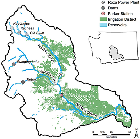
Figure 1. Location of reservoirs, irrigation districts, the Roza hydropower plant, and control point (Parker station) in the Yakima River Basin (Zhao et al., 2021).

Agriculture accounts for the majority of economic activity because of affordable land, fertile soil, and an ideal climate for growing crops with minimal disease issues. Many varieties of crops have been grown in the YRB. As of 2007 more than 50% of the total cropland (about 2.0 × 10⁹ m²) is used for orchards, hay, and forage (Washington State Department of Agriculture, 2013). Annual surface water demand for agriculture is 95% of the total surface water demand, which is supplied by natural flow, return flow, and 1.43 × 10⁹ m³ of total reservoir storage (USBR, 2011a). About 95% of the water is diverted from above Parker station (Figure 1). The lower YRB is able to meet its surface water demand from return flow, which is about 45% of the irrigated water which returns to the river system through groundwater discharge and surface runoff with different time lags (Vaccaro, 2011). Water loss on cropland due to crop evapotranspiration (ET) is estimated at 1.7 × 10⁹ m³ per year on average (17% of the total precipitation) and exceeds total water reservoir storage (Vaccaro and Olsen, 2009). Many recorded droughts have caused serious damage to the agricultural sector due to water curtailments and lack of storage capacity to buffer water supply deficiency.

Groundwater has become an important resource to support domestic use, environmental use, public water supply, and agricultural development. During drought years, groundwater withdrawal can account for 25% of the total irrigation water (Jones et al., 2006; USBR, 2011a). According to a report from the Washington State Department of Ecology (Vaccaro and Sumioka, 2006), there are more than 20,000 wells in the basin with associated groundwater rights. Groundwater rights in the YRB consist of 2,575 certificates, 299 permits, and 16,600 claims that collectively can withdraw about 815 km³ of water as reported by the Tri-County Watershed Resource Agency (TCWRA) in 2000. Eighty percent of the withdrawals is used for irrigation covering an area of 525 km².

Future climates

Five GCMs were chosen for future climate simulation forced by two RCPs, RCP 4.5 and RCP 8.5 (Field, 2014). RCP 4.5 describes an intermediate scenario and RCP 8.5 represents the worst scenario with aggressive fossil fuel usage that could cause significant global warming. These five GCMs were CanESM2 (Flato et al., 2000), GFDL-ESM2G (Dunne et al., 2012), HadGEM2-CC365 and HadGEM-ES365 (Collins et al., 2011; Martin et al., 2011), and INMCM4 (Volodin et al., 2010). We selected them by ranking 18 available GCMs based on their changes in average temperature and average precipitation from historical period (1980–2010) to future period (2030–2090) across the YRB (Malek et al., 2018a). Then, we selected 5 out of 18 GCMs for future scenarios that considered both average and extreme climate conditions (Table 1). The output of the GCMs were downscaled to gridded cells with 1/16 degree resolution on a daily time step using the Multivariate Adapted Constructed Analogs-version 2 (MACA2) described by Abatzoglou and Brown (2012).

TABLE 1

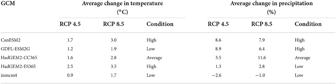
Table 1. The average projected change in temperature and precipitation for the five selected GCMS associated with RCP 4.5 and RCP 8.5 (Malek et al., 2018b).

The Palmer Drought Severity Index (PDSI) (Palmer, 1965) was used to evaluate the timing and drought severity for each GCM (Figure 2). PDSI is a widely used index to quantify long-term drought based on the water balance including anomalies in precipitation and ET, and soil water holding capacity (Vicente-Serrano et al., 2010). The PDSI can capture the impact of global warming on drought through projected changes in potential ET (Dai et al., 2004). However, PDSI assumes all precipitation is rainfall and it does not account for time-evolving storage, such as snowpack, which can affect drought status in snow dominant regions. For long-term projection of Yakima's drought condition, the first 20 years (2020–2040) are mostly wet years, followed by mixed dry and wet years during 2040–2060 and increased drought severity after 2060 for both RCP 4.5 and 8.5 (Figure 2) across different GCMs. We averaged the five GCMs within each RCP scenario to retain the main features of wet-median-dry patterns of future climate and focused on drought severity featured by RCP 4.5 and RCP 8.5 scenarios.

FIGURE 2

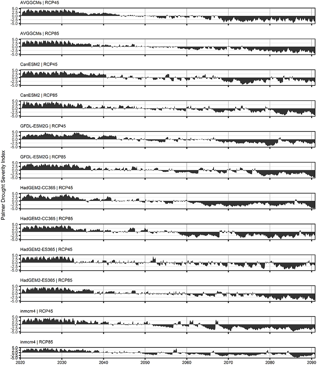
Figure 2. Palmer drought severity index (PDSI) for five GCMs and average of GCMs (top two: AVGGCMS) under RCP 4.5 and RCP 8.5 for future projection of 2020–2090 in the YRB. Positive PDSI indicates moist condition and negative PDSI indicates drought condition. Classification of PDSI follows extreme wet (≥4), normal (=0), and extreme drought (<= −4).

Methodology

Data sources

Naturalized inflow (non-regulated inflow from reservoir management) from the upper YRB (headwater regions) accumulating at Parker station was simulated by the VIC-CropSyst model (Malek et al., 2017) based on downscaled average GCM outputs, and this inflow was used as input to the SD model water system. Climate time series, including precipitation, actual ET, temperature of the gridded cell containing the Parker station (Figure 1), was used to represent the average future climate for crop lands in the YRB. All future climate data were projected from 2020 to 2090.

Historical data were used to provide daily averages for variables needed in the 2020–2090 period, such as hydroelectricity demand, which is a small component of reservoir management in the YRB. Data related to requirements and features for the YRB (USBR, 2011b), including Title XII target instream flow, surface water and groundwater rights, crop land areas, soil properties, reservoir maximum capacities, were the same as in Zhao et al. (2021). New data includes greenhouse crop coefficients and growth stages (Harel et al., 2014), evaporative cooling system water demand (Sabeh et al., 2006), maximum yield for apple and alfalfa crops (USDA, 2017).

Water storage management

System dynamics approach

A water storage management tool was developed and improved from Zhao et al. (2021) using the SD modeling platform Stella (iSee Systems, Inc., Lebanon, NH, USA). The tool captures processes and interactions of water allocation in the YRB based on incoming natural flow to current water storage and water demand from agriculture and hydroelectricity generation (Figure 3). We aggregated five reservoirs to one system water storage for water system operation following the priority to meet Title XII instream flow target (USBR, 2008), hydropower demand, and irrigation. The water system operation algorithm was based on total water supply for agriculture (TWSA), water demands from food, energy, and environmental instream flow, constraints of minimum and maximum water storage, flood season, irrigation season, and reservoir goal curve. The historical daily average of total reservoir storage above Parker station was used as the reservoir goal curve. Soil water dynamics played a critical role in deciding how much water was needed for irrigation according to crop growth season, water loss from ET, and irrigation efficiency level from the current irrigation system. Surface water diversion was the main supply source while groundwater was used as co-supply during non-drought years or backup supply in case of insufficient surface water supply during drought years. The use of both water resources was limited by surface water entitlements (i.e., proratable and non-proratable water rights) and groundwater entitlements (i.e., primary and standby water rights), respectively. The groundwater accumulated from MAR implementation was defined as “MAR entitlement” in this study, which is a type of water right to be used when both surface water and groundwater entitlements were exhausted. In addition to managed aquifer recharge (MAR), we developed new modules based on the SD model from Zhao et al. (2021), including greenhouse systems and crop production (section greenhouse system and crop yield), to evaluate possible management strategies to improve irrigation reliability as well as economic benefits. We chose the open field high and low value crops represented by apples and alfalfa, respectively, and tomato represented the greenhouse crop.

FIGURE 3

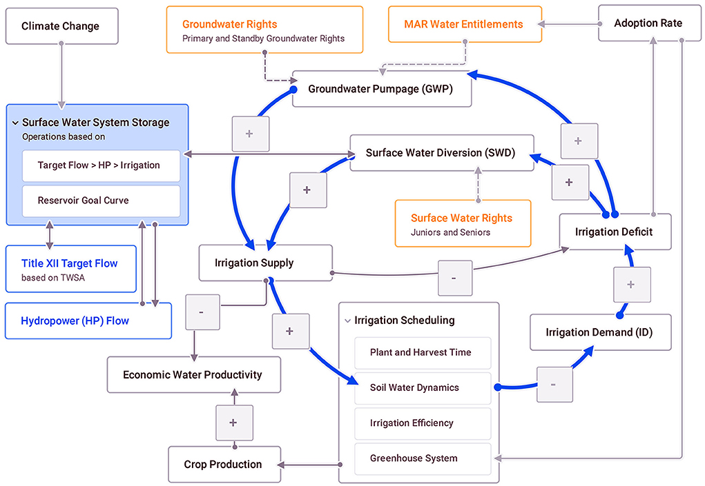
Figure 3. Conceptual map of the water storage management tool. The plus sign “+” indicates a positive relationship between two connected variables, where they change in the same direction, and the negative sign “–” means that two variables change in the opposite direction.

Greenhouse system

Greenhouse system water demand included water required for evaporative cooling systems and water loss due to ET. Evaporative cooling pulls outside air through a wetted pad and uses the heat from the air to evaporate water from pads for cooling purposes. The effectiveness of cooling depended on the ventilation rate of the fan system. An average water use of 0.18 m³/(m²·s) was assumed based on a 0.037 m³/(m²·s) air exchange rate (Sabeh et al., 2006). Daily air temperature ranged between the designed maximum (32.2°C) and minimum (18.3°C) temperature for growing crops (Shamshiri et al., 2018) to represent temperature fluctuation inside GHs. We used the Hargreaves method (Hargreaves and Samani, 1985) to calculate reference ET (ET₀) inside the greenhouse. Two year-round crop rotations for tomato were scheduled with a spring crop starting in January and a fall crop starting in July for 180 days per rotation. Crop coefficients (K_c) for spring and fall seasons are shown in Supplementary Table S2. Actual ET was calculated as the product of K_c and ET₀.

The adoption of GH systems was assumed to replace low value crops (i.e., alfalfa) due to considerable crop value difference and limited crop land areas. The land use density for GHs was at 80% with plants seeded at a density of 2.5 plants/m². Greenhouses used water tanks for flexible water supply. More water was allocated to the GH storage tanks when water demand exceeded the management allowable depletion (MAD) of the tank storage at 90%. Precipitation was another source for GH water collection and 5% of the total precipitation falling on the GH area was assumed to be stored in the tanks. The GHs were assumed to be closed hydroponic systems with 100% water use efficiency.

Greenhouses had the priority to divert water from total water allocation, and the rest was diverted to crops for open fields. The total irrigation demand included water demand from apple, alfalfa, and tomato growing (Figure 4). Final total water allocation depended on water system operation rules described in section system dynamics approach. Adopted GH area was a function of an adoption ratio calculated based on the innovation diffusion model (Sterman, 2000; Repenning, 2002) with additional impact factors (Zhao et al., 2021), such as drought severity stimuli and the effectiveness of the adoption method. As farmers switched alfalfa for GHs (Figure 4), a reinforcing causal loop (Loop R) and a balancing causal loop (Loop B1) controlled the behavior of adoption rate for GHs depending on whether GHs can help mitigate the drought impact on water scarcity for irrigation.

FIGURE 4

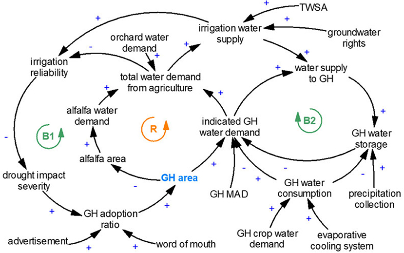
Figure 4. Causal loop diagram for greenhouse system within irrigation water demand and supply structure. B denotes balancing loop; R denotes reinforcing loop.

Crop yield

Crop yield, defined as crop production per unit area, was mainly affected by crop water use through actual ET. Generally, there is a positive relationship between yield reduction and reduced soil moisture content as a result of water supply shortage (Doorenbos and Kassam, 1979). We calculated crop yield for apple and alfalfa with Equations (1) and (2) that describe the yield response to actual ET (Steduto et al., 2012). Greenhouse crop yield was assumed constant [28.2 kg/m² (OSU Extension Service, 2002)] representing the average yield for two growing seasons together.

$\begin{array}{ll}{Y}_a=Y_x\left[1-K_y\left(1-\frac{E{T}_a}{E{T}_x}\right)\right]& (1)\end{array}$

$\begin{array}{ll}E{T}_x=K_{c}E{T}_0& (2)\end{array}$

where Y_a is actual crop yield; Y_x is the maximum crop yield; K_y is a yield response factor indicating the sensitivity of yield reduction to ET reduction; ET_a and ET_x are the actual and maximum ET. Based on data from the United States Department of Agriculture (USDA, 2017), maximum crop yields for apple and alfalfa were fixed at 5.4 and 1.64 kg/m², respectively. K_y was 1.1 for alfalfa and 1 for apple (Steduto et al., 2012). ET_a was calculated based on soil water dynamics in the irrigation supply module of the model.

Model calibration and validation

We used the total reservoir storage and observed daily streamflow at Parker station during 1979–1999 to calibrate the model after adding new modules and improving the algorithm of water system operations based on the SD model version in Zhao et al. (2021). Then, we validated the model with the same variables for the next 15-year time period (2000–2015). Calibration used the embedded Powell optimization tool (Powell, 2009) in Stella. Model performance for validation used the Nash-Sutcliff Efficiency (NSE) coefficient (Nash and Sutcliffe, 1970). In addition, we evaluated the performance using RMSE and R² (see Supplementary material).

$\begin{array}{ll}NSE=1-\frac{{\displaystyle {\sum }_{i=1}^n}{\left(Q_{obs,i}-Q_{sim,i}\right)}^2}{{\displaystyle {\sum }_{i=1}^n}{\left(Q_{obs,i}-\overline{Q_{obs}}\right)}^2}& (3)\end{array}$

where Q_obs and Q_sim are the observed and simulated values, respectively; $\overline{Q_{obs}}$ is the average of the observed value; n is the number of data points.

Scenario analysis

Climate conditions

Future climate showed a wet-to-dry trend with different levels of wetness and dryness at different time periods. We divided the 70-year climate projection (2020–2090) into seven decades to represent future climate conditions (CCs) similar to Malek et al. (2018a). Historical climate from 1979 to 2015 served as a baseline, while relative changes of precipitation and temperature for each CC relative to the baseline mostly increased from 2020 to 2090 (Table 2). Severe drought conditions are likely to occur with increased average temperature and decreased average precipitation. RCP 8.5 had more intense CCs with greater relative increases in temperature, compared to RCP 4.5.

TABLE 2

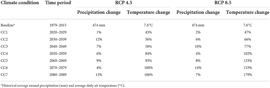
Table 2. Relative changes in average annual precipitation and temperature from each climate condition to historical average (1979–2015) of precipitation and temperature.

Each CC could occur in the future instead of following the specific timeline simulated from GCMs. Managers and stakeholders can optimize a ten-year water conservation plan facing each possible CC for their various combinations and levels of droughts. Long-term plans can also be evaluated by using the 70-year climate projection (see section impact of adoption in long-term management).

Water management for each climate condition

Agriculture in the YRB is relatively vulnerable facing water scarcity because irrigation heavily depends on climate conditions. From historical records during 1979–2015, droughts occurred seven times with proration rate lower than 70%. Failure of sufficient water supply during droughts resulted from mismatch between demand and supply, such as the lack of reservoir storage (insufficient supply) and inefficient irrigation systems (high demand). Drip and sprinkler irrigation methods are favored by orchard owners in the YRB, and drip irrigation only covers a small portion (13%) compared to sprinkler systems (49%). Inefficient methods, such as rill and flood irrigation (36% of total irrigated land) are still common especially in the Kittitas valley and lower valley of the YRB (Johnson, 2000). In the model, the average irrigation efficiency (IE) was assumed to be 0.75 based on all irrigation methods in the YRB.

To reduce the vulnerability to droughts, we propose four climate adaptation methods for water management that either reduce irrigation demand or increase irrigation supply. The selected adaptation methods include GHs, shifting crop planting time to earlier in the season, irrigation technology for IE improvement, and managed aquifer recharge (MAR). For MAR, this study only considered surface recharge by delivering water through existing canals and spreading water on agricultural land for infiltration and percolation. We listed the measurement for each method to represent their adoption levels (Table 3). Greenhouse adoption was measured by the fraction of land switched from alfalfa to GHs, named GH area fraction (GHAF). Management for crop planting time shift (PTS) was measured with days where positive values of shifted days indicated planting crops earlier relative to the default planting date (at day 92 from the beginning of a year for alfalfa). The crop growing season length was unchanged (208 days). Improvement in irrigation technology (IT) was measured by the average IE, which was defined as the ratio of actual water stored in the root zone of open field crops (apple and alfalfa) vs. water delivered for irrigation. MAR was measured by the infiltration area (IA) with a constant infiltration rate (0.43 m/day) and hydraulic conductivity (1.52 m/day) (Zhao et al., 2021). The initial available MAR entitlement was set at 0.1 × 10⁹ m³ for RCP 4.5 and 0.5 × 10⁹ m³ for RCP 8.5 to spin up the adoption of MAR (Zhao et al., 2021). This was also to overcome the fact that MAR application was a time-dependent method.

TABLE 3

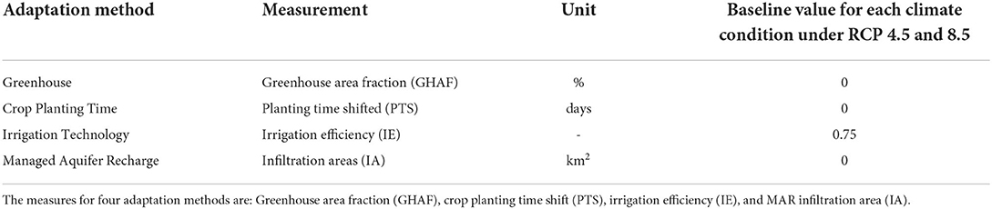
Table 3. Baseline values for four methods in their measurement units.

In this CC analysis, we used the model to find the minimum requirement for each of the four adaptation methods that can fully mitigate drought effects on irrigation for each CC under RCP 4.5 and 8.5, while keeping other methods unchanged from the baseline (Table 3). The minimum requirement was defined as an application level of an adaptation method that improved irrigation reliability to 1 (irrigation water supply met irrigation demand) for every year within the selected CC. For example, when 15% of the total alfalfa land switched to GHs (GHAF = 15%), the water shortage for agriculture resulting from droughts was fully mitigated for CC1 under RCP 4.5. Thus, a GHAF at 15% was the minimum requirement for CC1. It was assumed that each CC represented an independent, ten-year planning window not affected by other CCs. For all CCs, we calculated the precent change from baseline in agricultural water demand and supply resulting from each adaptation method. Greater percent change indicated greater sensitivity of demand or supply dynamics to the adaptation method.

Impact of adoption in long-term management

Long-term planning required consideration of the outcomes from adopting proposed adaptation methods. Innovation adoption describes a predictable process of innovative methods being adopted within a given community. We assume adoption behaviors are affected by advertisement, word of mouth, effectiveness of adaptation methods, cost-effective driven adoption, and drought stimuli, explained in Zhao et al. (2021). Effectiveness of adaptation methods in mitigating drought impact on irrigation reliability was evaluated differently for each method: (1) for GH, the ratio of reduction in ET loss to total ET loss; (2) for MAR, the ratio of MAR supply to water demand deficit (i.e., demand that is not met by water supplied without MAR); (3) for IT, the ratio of water saved from improving irrigation efficiency to total water supply. Adoption behaviors vary over time as the drought tolerance changed as a result of implementing adaptation methods. Cost-effective driven adoption was to reflect the fact that cheaper infrastructure tends to be diffused faster, which was assumed as MAR > IT > GH. We analyzed the role of adoption behaviors in drought mitigation from 2020 to 2090 with the initial adoption ratio at zero in 2020.

Adoption ratio is the ratio of the number of adopters over the total amount of potential adopters. Thus, adoption ratio approaching 1 indicates that the adopters approach the total population (e.g., irrigation units). We defined maximum threshold for the measurement of each adaptation methods, including GHAF, MAR IA, and IE, to represent the limitations of financial and natural resources. For example, infiltration area at full adoption (IAFA), defined as the maximum infiltration area at a 100% adoption ratio, is an upper threshold for MAR measurement. The upper thresholds for measurements were 70%, 3.0 km², and 0.95 for GHAF, MAR IA, and IE, respectively. The lower thresholds were baseline values (Table 4), and the measurement value at time t for each adaptation method was calculated by Equation (4). Five scenarios were designed to evaluate the impact of individual methods and combined methods on drought mitigation (Table 4) under RCP 4.5 and 8.5.

$\begin{array}{ll}{M}_i^t=T{H}_{min,i}\left(1-r_i^t\right)+T{H}_{max,i}{r}_i^t& (4)\end{array}$

where $M_i^t$ is the measurement value at time t for method i, i = GH, MAR, or IT; TH_{min, i} and TH_{max, i} are minimum and maximum threshold for the measurement of method i, respectively; $r_i^t$ is the adoption ratio for method i at time t, which is the ratio of irrigation units that adopt method i over total irrigation units. $r_i^t=0$ means no irrigation unit adopts the method i at time t; $r_i^t=1$ means all irrigation units adopt the method i at time t.

TABLE 4

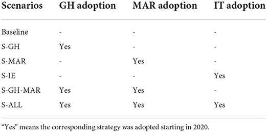
Table 4. Description of five scenarios on the adoption status, compared to the baseline.

System resilience and sustainability indicators

Four indicators were selected to show the outcomes of adopting various management strategies from different perspectives, including irrigation reliability (IR), groundwater supply fraction, crop production, and economic water productivity (EWP, see Supplementary material). We used these indicators to demonstrate the critical factors that may affect system resilience and sustainability in terms of environmental resources and economic values.

IR is an index for the total agricultural water supply (AWS) and agricultural water demand (AWD) ratio in terms of open fields and greenhouses consuming surface water and groundwater. The IR was calculated at an annual time step based on the concept of volumetric reliability (Hashimoto et al., 1982; Kundzewicz and Kindler, 1995).

$\begin{array}{ll}IR=\frac{AWS}{AWD}& (5)\end{array}$

Groundwater supply fraction (referred to as F_GW) was defined as the proportion of groundwater supply (GWS) pumped for agriculture in AWS Equation (5), indicating the irrigation dependence on groundwater as well as the level of available groundwater entitlements and surface water availability. For example, more groundwater would be pumped for irrigation purposes when surface water supply cannot keep up with crop water demand due to drought. The groundwater supply fraction was calculated on an annual basis.

$\begin{array}{ll}{F}_{GW}=\frac{GWS}{AWS}& (6)\end{array}$

Results and discussion

Model performance evaluation

Model simulations during the evaluation period (2000–2015) agreed well with the observed total reservoir storage and streamflow at Parker station, using parameters calibrated during 1979–1999. The simulated system water storage captured peak storage and low storage levels well, except for a few years (e.g., 2001) where simulations indicate more intense water releases during the irrigation season as compared to observed releases (Figure 5). For streamflow at Parker station, the model performed well-during most dry and flood seasons. Few overestimated low flows and underestimated high flows were caused by storing extra water in the reservoir during flood seasons, compared to observed daily reservoir storage. Figure 5B shows the comparison of monthly reservoir storage and release between observations and simulations. Simulated reservoir operations, driven by climate, irrigation water demand, and water rights, tend to release slightly more water during the irrigation season, draining reservoir storage faster than observed. Irrigation water delivery was limited by surface water rights, and most underestimations of irrigation delivery in the model relate to surface water rights used up at the end of the month. For daily simulations, the NSE for the calibration period was 0.67 for streamflow and 0.85 for total reservoir storage. The NSE values decreased slightly to 0.57 and 0.74 for evaluation period, respectively.

FIGURE 5

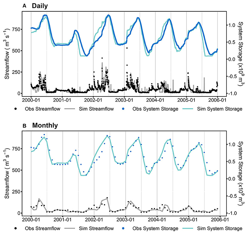
Figure 5. Simulations and observations of total reservoir storage and streamflow at Parker station for (A) daily values; and (B) average monthly values.

Management requirement for each climate condition

Features of climate conditions

Climate conditions included various drought features due to the timing and level of precipitation and temperature, which represent possible situations water resource managers may face in the future. The annual IR indicated drought severity, with the lower IR meaning a more severe drought (Figure 6). At baseline for RCP 4.5, the occurrence of droughts started to increase in the late 2040s and the possibility of more frequent and extreme droughts was high in 2060s and 2070s. The baseline for RCP 8.5 showed a clear trend of increasing drought severity after the late 2040s, and the average IR value was < 0.25 after the 2070s. Among seven climate conditions under each RCP scenario, the lowest average IR was during CC6 (2070s) under RCP 4.5 and CC7 (2080s) under RCP 8.5. However, the worst annual IR was during CC5 (2060s) under RCP 4.5. CC1 (2020s) and CC2 (2030s) for both RCP 4.5 and 8.5 appeared to be water sufficient and no action was needed for improving system water reliability. Overall, climate patterns within the CCs determined the water scarcity situations, where consecutive droughts would lead to a worse situation than if the same numbers of droughts spread within a decade.

FIGURE 6

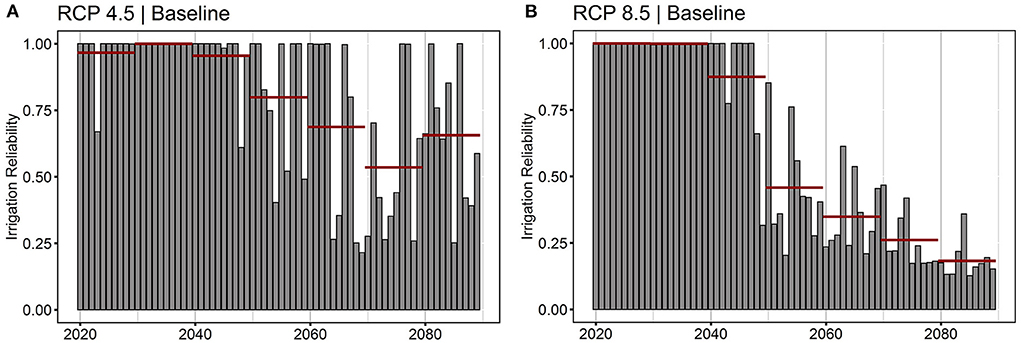
Figure 6. Annual irrigation reliability for (A) RCP 4.5 and (B) RCP 8.5. The red lines are the average irrigation reliability value for each CC. Lower irrigation reliability means there is not enough agricultural water supply to meet demand.

Management requirements

The minimum requirement for each adaptation method varied significantly under different CCs (Table 5). Higher values for the minimum requirement of adaptation methods indicated more resources (i.e., financial, land, and permits) were needed to alleviate drought impacts on irrigation. There were no minimum requirements for all four methods under CC2 for both RCPs due to the wet climate. For CC5 under RCP 4.5, the minimum requirements for GH, crop PTS, and IT were all the highest, compared to requirements in other CCs. However, infiltration area for MAR was higher at 4.1 km² for CC6 than 2.7 km² for CC5 because temporal distribution of severe droughts was mostly at the first half of CC6 whereas droughts in CC5 occurred in the second half of the decade. This indicates that MAR depended on the long-term efforts to accumulate MAR entitlements and were more valuable at longer planning times. GHAF needed to take over more than 50% of the low value croplands to improve drought conditions for CC5–CC7. The minimum requirements of PTS ranged from day 0 to 73, which illustrated that moving crop planting time to late January can significantly drop the water demand level due to lower ET in the winter season. Improving IE appeared to be an effective method as minimum requirements for IE for most CCs were under 0.9, which can be achieved easily by switching from traditional flood irrigation to sprinkler and drip irrigation.

TABLE 5

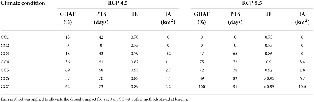
Table 5. The minimum management requirement for each method.

The minimum requirements for all four adaptation methods were much higher under RCP 8.5 than RCP 4.5 as a result of the higher frequency of severe droughts (Table 5). The most extreme CC7 required the highest application level of GHAF or IE reach for drought mitigation. However, even the highest level of IE of 0.95 was not able to fully secure agricultural water supply. Crop PTS needed to move more than 2 months earlier, in order to reduce water demand; however, crop yield may drop significantly as other agronomic factors other than water affect crop growth when planted in winter. MAR IA under CC7 was more than three times that under CC4, with 10.6 km² of IA needed to accumulate ~ 5.1 × 10⁹ m³ of MAR entitlement in a decade. Overall, RCP 8.5 created challenging CCs and each CC required well-defined infrastructures for adaptation methods to improve water security.

The minimum requirement identified the potential implementation scale for each method. Most of the extreme requirements were to evaluate the degree of effort needed using a single adaptation method without knowing if these would be entirely realistic in future settings. For example, switching 100% of low value cropland to GHs exemplifies the severity of droughts in terms of GH implementation scale. However, all the minimum requirements may not be met due to limited natural and financial resources, environmental feasibility, and applicability. For example, considering damages from first frost/freeze, over-moist soil in the early growing season, and limited growing degree-days for proper crop development when spring alfalfa is sown in winter, the higher value of crop PTS may not be valid. Alternatives can include planting cool season crops in the fall for winter/spring harvest to achieve the goal of ET reduction. However, evaluation of cropping patterns and practices were beyond the scope of this paper.

Impact of adaptation methods on agricultural water demand and supply

All four adaptation methods reduced irrigation demand by 5–80% under most CCs (Figure 7). A positive relationship exists between drought severity and agricultural water demand reduction under adaptation management. For example, percent change in water demand reduction for CC2 under both RCP 4.5 and 8.5 was 0 because water demand was already satisfied by available supply (Figure 6) without any adaptation methods. In contrast, the highest percent change in water demand reduction for RCP 4.5 was in CC6 as a result of its extreme water scarcity status. Similarly, under RCP 8.5, water demand from CC3 to CC7 showed a decreasing trend relative to the baseline in all adaptation methods except for IE management in CC7. This was because IE reached its maximum threshold (0.95) in CC7, but the method was still unable to erase all the drought impacts.

FIGURE 7

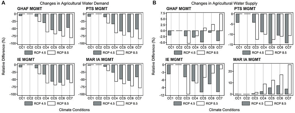
Figure 7. Percent change from the baseline in (A) agricultural water demand and (B) agricultural water supply under all CCs for each adaptation method under RCP 4.5 and 8.5.

The reduction level of agricultural water demand was dependent on the adaptation method being used. In fact, drought created a situation where the soil water content kept decreasing with continuous water loss from ET and insufficient irrigation, leading to increasing water demand over time. All methods directly or indirectly reduced water demand in three ways: (1) reduced biological water demand of crops from reducing ET (e.g., PTS); (2) reduced irrigation water wasted (e.g., IT, GH); and (3) reduced soil water deficit by increasing supply (e.g., MAR). Adaptation methods, such as PTS, whose purpose was to decrease crop water demand, had the most reduction compared to others (Figure 7). Shifting planting time earlier reduced ET due to increased growing days during winter season, where ET remained low compared to ET in summer. In addition, earlier harvest avoided high risks of having limited water during summer.

Agricultural water supply mostly decreased with application of adaptation methods except for GHs and MAR (Figure 7). The most reduction was from crop PTS in CC5 at about 14% under RCP 4.5 and 13% under RCP 8.5. Agricultural water supply and demand depended on each other via soil water dynamics, for example, reduced demand led to less supply. However, MAR, as an exception, increased water supply because MAR created extra water storage for emergency use. GHs resulted in mixed positive and negative changes of relative difference in water supply under RCP 8.5 (CC5–CC7). This is because increased GHAF led to contradictory consequences on water supply according to feedback relationship shown in Figure 4. On the one hand, reduced alfalfa acreage greatly reduced ET losses, and thus reduced water supply. On the other hand, GHs required more consistent water supply throughout the growing season with water storage infrastructure, which allowed more water to be stored for use during droughts.

Long-term impact of innovation adoption

The adoption rate of innovations and new policies changes by time and is driven by the number of potential adopters, information dissemination, social norms, and various factors. Generally, adoption behavior follows a S-shaped growth curve with few early adopters (Sterman, 2000). The large base of assumed potential adopters is one of the drivers for fast growth in the initial stage if there is positive feedback (Bass, 1969). However, the innovation diffusion may take many years to reach a 100% adoption ratio and it is important to consider the time needed to improve agricultural water conservation and management strategies for climate change adaptation. We now describe the impact of adoption on three adaptation methods, including GHs, IT, and MAR, and the effectiveness of long-term adaptation strategies on improving water sustainability under climate change.

Agricultural water demand and irrigation reliability

The most effective individual methods for reducing irrigation deficit were MAR for RCP 4.5 and GHs for RCP 8.5, respectively, whereas a combination of all the adaptation methods (S-ALL) achieved the best results (Figure 8). The reduction of irrigation deficit can be the result of decreased irrigation demand or increased irrigation supply. In the baseline of RCP 4.5, the agricultural water demand reached a peak value of around 12 × 10⁹ m³ in the 2060s and remained high in the next two decades, compared to a value around 2.5 × 10⁹ m³ before 2050. In the baseline of RCP 8.5, the median annual water demand by decade started to increase from 2050s at an average rate of 3 × 10⁹ m³ per decade. Most water demand ranged from 13 to 18 × 10⁹ m³ in the 2080s, which is about seven times the median water demand of 2.5 × 10⁹ m³ in the 2020s. With intense water shortage in the second half of the century, both GHs and IE were effective and lowered annual water demand for RCP 8.5 to around 5 × 10⁹ m³, compared to the MAR. With the combination of GH and MAR or all three methods, the water demand slightly decreased with time for both RCPs, which can be used as an effective and flexible strategy to mitigate drought when a certain method has limitations.

FIGURE 8

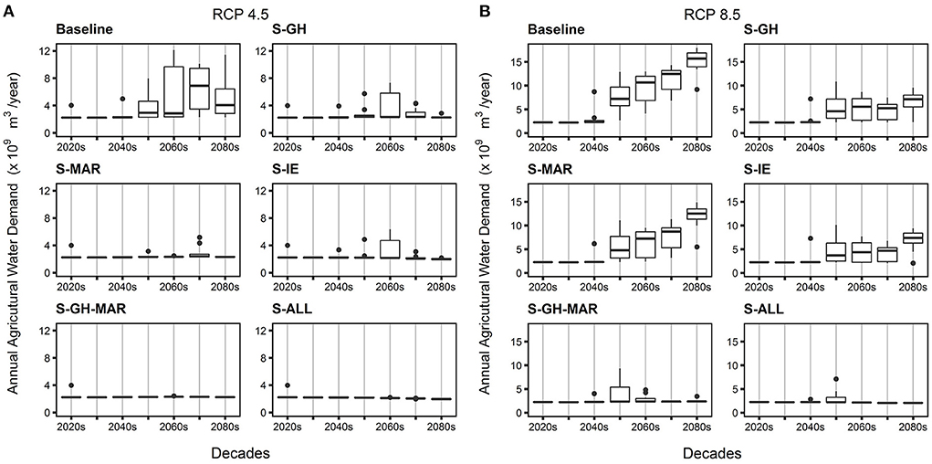
Figure 8. Impact of adopting individual and combined adaptation methods on annual Irrigation demand under (A) RCP 4.5 and (B) RCP 8.5.

We selected two different dry periods for RCP 4.5 (2070–2075) and 8.5 (2080–2085), respectively, to demonstrate the impact of adaptation methods on dynamics of soil moisture content (Figure 9). During typical dry years from 2070 to 2075 for RCP 4.5, the water loss by ET led to a soil moisture content drop below 15% at baseline. The soil was even drier during 2080–2085 under RCP 8.5 indicating considerable water stress from extreme droughts. Among three single method scenarios, GHs restored soil water the most during these periods for both RCPs, followed by IT and MAR. MAR filled up soil water to field capacity during 2070–2073 with the remaining available entitlements and became less effective even if its adoption ration was approaching 1.0. Soil moisture content was the bridge connecting agricultural water demand and supply. Agricultural water demand kept increasing when the deficit between current soil water content and field capacity was not replenished, which put more pressure on future supply. The key to mitigate drought conditions was continuously wetting the soil or slow down the water loss from the soil to avoid increased soil water deficits. Different adaptation methods can be more helpful for certain climate patterns according to their basic principles in mitigating droughts.

FIGURE 9

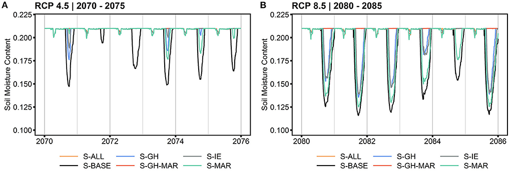
Figure 9. Impact of adaptation methods on soil moisture content during (A) 2070–2075 under RCP 4.5 and (B) 2080–2085 under RCP 8.5.

The results of annual irrigation reliability show a finer temporal resolution of the impact of adaptation methods on extreme future climates (Figure 10). All adaptation methods performed better in improving irrigation reliability under RCP 4.5 than under RCP 8.5. Under RCP 4.5, both IT and GHs appeared to be less effective than MAR. Under RCP 8.5, GHs and IT served as a better option in increasing irrigation reliability with frequent severe droughts. The discrepancy of effectiveness of adaptation methods under RCP 4.5 and RCP 8.5 was because of their fundamental functionalities, where GHs and IT were methods focusing on reducing water demands and MAR was focusing on increasing water supply. By switching low value cropland to GHs, higher water use efficiency in GH's irrigation system decreased average water demand overall. Improving IE directly increased the volume of water stored in the crop root zone per unit volume of water irrigated to the soil. MAR did not significantly enhance water scarcity conditions after 2050 for RCP 8.5 as a result of low adoption rate at the initial stage as well as high consumption of MAR entitlements during 2050s. With all adaption methods working together, we still see there were 4 years having water shortages in 2050s due to low adoption rate (0.1–0.3) in the middle of the century.

FIGURE 10

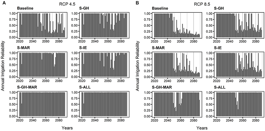
Figure 10. Annual irrigation reliability for scenarios adopting individual method and combined methods on under (A) RCP 4.5 and (B) RCP 8.5.

MAR adoption ratios increased faster than the adoption ratios for IT and GH and the more extreme climate in RCP 8.5 encouraged greater adoption in a shorter time for all adaptation methods (Figure 11). Note that the values at the full adoption for GHs, IT, and MAR were 70% of the alfalfa land, IE at 0.95, and IA at 3.0 km². The actual adoption for each method started low and increased as more and more irrigation units decided to take action to improve water security. MAR was assumed as an easier adaptation method than the other two methods because no extra construction was needed to apply MAR. However, the reason of MAR failing to provide enough groundwater under RCP 8.5 (Figure 10) was due to low available MAR entitlement with low infiltration area. With a MAR area of 3.0 km² at full adoption, the IA increased to 0.36 km² and accumulated 0.15 × 10⁹ m³ of water entitlement at around year 2048 (Figure 12), when severe droughts under RCP 8.5 started to occur. Therefore, the speed of MAR entitlement accumulation could not catchup with agricultural water demand, so that the entitlement dropped to 0 in 2050 and stayed low after that. On the other hand, the same designed IAFA under RCP 4.5 could always satisfy almost all the agricultural water demand and managed to retain a good amount of groundwater entitlement by the end of the century. The entitlement accumulated as high as 0.8 × 10⁹ m³ in 2064 and declined sharply due to a dry climate for 10 years. As a cost-effective adaptation method, our findings suggest an appropriate MAR design for IAFA based on the projected CCs, the capacity of the groundwater system, and available land for infiltration can mitigate drought impact by providing large buffers for climates with alternate dry and wet conditions.

FIGURE 11

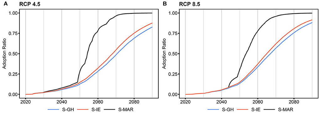
Figure 11. Adoption ratio for three adaptation methods under (A) RCP 4.5 and (B) RCP 8.5.

FIGURE 12

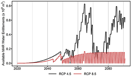
Figure 12. Available MAR water entitlements if MAR were implemented in 2020 with 3.0 km² as targeted infiltration area at full adoption under RCP 4.5 and RCP 8.5.

Groundwater supply fraction

Groundwater is an important and vulnerable resource in water supply. Increasing groundwater use in total water supply can cause dramatic groundwater depletion when the average pumping exceeds average recharge rate. GHs and IT indirectly reduced the groundwater supply fraction (F_GW) especially in later decades under RCP 4.5 (Figure 13). MAR as a groundwater resource kept F_GW as high as the baseline level. However, groundwater pumped from available MAR entitlements was artificially recharged from surface water thus using the aquifer as extra storage which was less likely to cause negative effects on groundwater levels.

FIGURE 13

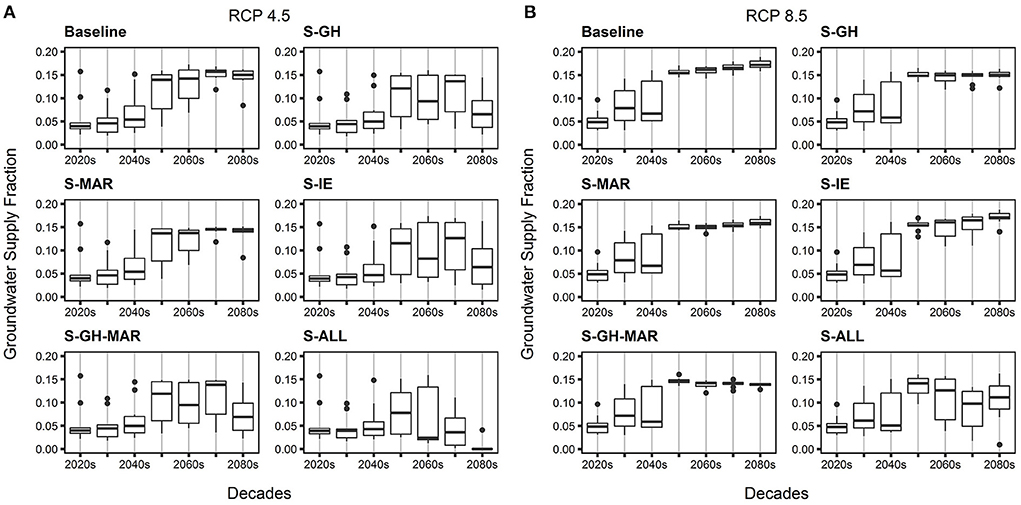
Figure 13. Ground water fraction for scenarios adopting individual method and combined methods under (A) RCP 4.5 and (B) RCP 8.5.

The result for RCP 8.5 showed that a combination of all methods was needed to lower the F_GW (Figure 13). The F_GW during 2020–2060 was not affected very much even with application of all adaptation methods. However, all adaptation methods combined greatly reduced the median of F_GW in last three decades especially for 2080s, the decade with the highest F_GW in baseline. During severe drought scenarios, all annual groundwater rights were mostly consumed during the summer season and time periods when irrigation water rights were not available (outside of Apr–Oct). With the help of all adaptation methods, groundwater pumping was shifted mainly before April and after September serving as a backup for limited surface water.

Crop production

RCP 8.5 had more impact on crop production than RCP 4.5 for both low value (e.g., alfalfa) and high value (e.g., apple) crops (Figure 14). Average annual production of alfalfa in each decade at baseline fluctuated around 0.62 × 10⁶ tons/year before the 2050s and reduced gradually after the 2050s, especially for RCP 8.5. MAR and IT slightly increased alfalfa production relative to the baseline. GH implementation led to a significant drop in alfalfa production to 0.25 × 10⁶ tons/year on average due to reduced land area for alfalfa for both RCPs. Apple production was also sensitive to the increasing GHs adoption. For RCP 4.5, adopting GHs increased high value crop production from an average of 3.0 × 10⁶ tons/year in 2030s to 3.1 × 10⁶ tons/year in 2080s, compared to baseline with decreased production after the 2040s to as low as 2.75 × 10⁶ tons/year in 2070s. MAR and IT slightly improved apple production by 0.2 × 10⁶ tons/year on average during droughts. For RCP 8.5, apple production at the baseline showed an obvious reduction associated with the increasing trend of frequency and severity of droughts. Similar to RCP 4.5, GHs was more effective at improving apple production as adoption increased for RCP 8.5. For example, about 62% of GHAF (adoption ratio = 0.88) enhanced apple production by 0.5 × 10⁶ tons/year in 2080s from the baseline. During 2060–2090 with frequent extreme droughts, IT increased apple production by 0.4 × 10⁶ tons/year on average, whereas MAR achieved the smallest average amount at 0.2 × 10⁶ tons/year. With all three adaptation methods, we can only see a slightly increasing trend of apple production toward the end of the century.

FIGURE 14

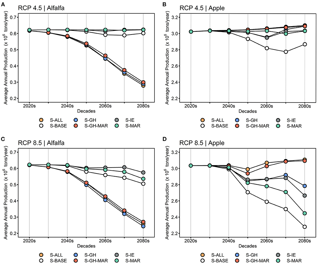
Figure 14. Average annual crop production within each decade for apple and alfalfa under six scenarios for (A,B) RCP 4.5 and (C,D) RCP 8.5.

The critical time in the year determining the amount of annual crop yield was the end of the growing season when drought impacts had accumulated as expressed by lack of water in the root zone. Lack of soil water reduced actual ET, leading to yield reduction according to Equation (1). The reason that GH was more effective in improving high value crop production was the reduced land area in alfalfa (and thus reduced total water demand) and GH water demand. With sharing water with alfalfa and ET loss from alfalfa, the soil water in the root zone was used up faster, which exhausted the water supply system more quickly during the irrigation season. Consequently, the orchard soon reached soil water deficiency in the middle season causing yield reduction. Without alfalfa, water available per unit open field for orchard increased allowing sufficient water in the root zone for ET demand. Improving IE increased the ratio of water stored in the root zone per unit water delivered to the field. However, this method had a ceiling that constrained the maximum irrigation efficiency. During extreme droughts, scenarios with high GHAF proved to be a better strategy to decrease water loss by ET.

Conclusions

In this study, a water system management tool evaluated the impacts of climate change on future water availability for agriculture. Following calibration-validation, the SD model simulated water system operations based on the basic future climate data including natural inflow, precipitation, and temperature projected with GCMs under RCP 4.5 and 8.5. The model included modules for greenhouses and crop yield based on the version from Zhao et al. (2021) to provide capabilities for evaluating innovations of water management strategies under climate change scenarios.

Without any adaptation measures, the probability of occurrence of annual irrigation reliability below 0.7 was more than 36% within the 2020–2090 time period under RCP 4.5. For RCP 8.5, irrigation reliability dropped below 0.5 for more than 40 years in the same time period. Low water availability under climate projections created difficult water supply conditions for agricultural activities. Clearly, water conservation and management strategies will be needed to overcome the impact of climate change on agriculture in arid climates like that in the YRB. More broadly, adaptive water management can be applied to regions with various patterns of water scarcity, such as those caused by heterogenous distribution of water resources and demands driven by socioeconomic growth (Wild et al., 2021a).

We evaluated four adaptation measures, including GHs, crop PTS, IT, and MAR, to find their minimum management requirements under seven CCs. With CC causing extremely dry conditions, more resources, such as land area for MAR and updated irrigation systems, were needed to overcome water scarcity. Climate Condition 5 under RCP 4.5 and CC7 under RCP 8.5 were the scenarios with frequent severe droughts, which mostly required the highest GHAF (69% and 100%), PTS (73 and 91 days), IE (0.95 and 0.95), and MAR IA (4.1 and 10.6 km²).

Assessment of the impact of adoption behavior on the effectiveness of three adaptation methods (GHs, IT, and MAR) starting from 2020 showed that the adoption ratio and adopted time length for each method played an important role in the effectiveness of adaptation methods under projected CC. MAR can be very effective if designed IAFA was enough to accumulate enough entitlements. However, available entitlements were used up once it reached a peak value in 10 years under RCP 4.5 and 2 years in RCP 8.5 with designed IAFA of 3.0 km². MAR was a temporal and spatial scale dependent adaptation methods, which did not change the amount of water demand based on crop type and crop land area. Updated irrigation system technology helped with decreasing water demand by efficiently putting more water into the root zone with less irrigated water. However, with the upper limit of water that can be saved by technology innovation, the improvement of IE, was also constrained to a certain extent.

Greenhouses proved to be the most effective adaptation methods among all methods under CCs when widely adopted. It reduced the agricultural water demand by switching low value cropland to GHs, which were equipped with more efficient irrigation systems that required much less water for two harvest cycles in a single year. Irrigation reliability improved the most for S-GH scenarios (or combined S-GH-MAR and S-ALL) in the decade with the most severe drought situation under RCP 8.5 at lower adoption ratios, compared to other measures (2080s). In addition, apple production increased about 11% under RCP 4.5 and 20% under RCP 8.5 in the 2080s, compared to the baseline with no GH adoption. The EWP jumped up about 15 times with the production of high value crops from the GH in the 2080s, compared to baseline (see Supplementary material).

This paper evaluated the effectiveness of potential adaptive management in mitigating droughts under projected climate change scenarios using SD framework. Assessing adaptation strategies for resources management under climate change requires holistic understanding of the system and agile perspectives (Gregory et al., 2006; Lawler, 2009). System-specific models and tools are developed to accomplish this goal. While it is not straightforward to compare structures and designs of an applied framework for different systems in adaptive water resources management, conclusions from multiple studies using a SD framework suggested the necessity of mixed strategies to manage water demand and supply in coordination to alleviate climate-induced droughts (Stave, 2003; Sahin et al., 2016; Gohari et al., 2017; Naderi et al., 2021).

Limitations and future potential improvements are discussed for this study. First, we applied the SD model to identify interactions, feedback, and delays while tracking water balances within a complex system such as the YRB. This process can involve different types of uncertainties in input data, model structure, parameters, and boundary conditions. Differences in assumptions and values from alternative sources can affect the results (Winz et al., 2009; Mirchi et al., 2012). As we validated the model's performance, the ultimate judgement of the model's usefulness should rely on its ability to answer related questions and to bring insights to the involved parties. The transparency of the SD model makes it possible for users to modify the model based on their judgements. Second, we did not consider cost constraints explicitly but generally the construction and maintenance costs for three methods was reflected in the adoption process and ranked as MAR < IT < GHs. With that in mind, the combination of shared lands for GHs and MAR could be designed considering future climate change and available budgets, along with upgrading from current rill and flood irrigation to drip or sprinkler systems in the YRB. Findings of this study also suggest that the adoption ratio was a key factor. Preventive actions can be taken by advertising or providing subsidies for stakeholders to adopt innovative methods in anticipation of future uncertainties.

Data availability statement

The data presented in this study are available on request from the corresponding author.

Author contributions

MZ and JB contributed to conception and design of the study. MZ collected and managed the database, developed the model, performed the analysis, wrote the first draft of the manuscript. All authors contributed to manuscript revision, read, and approved the submitted version.

Funding

This work was funded by the National Science Foundation (NSF) Earth Sciences (award #1639458) and the United States Department of Agriculture (USDA) (award # 2017-670 04-26131).

Acknowledgments

This work was conducted at Washington State University. We acknowledge Dr. Jennifer Adam, Dr. Keyvan Malek, and Dr. Mingliang Liu for providing data and VIC-CropSyst model simulations in the YRB.

Conflict of interest

The authors declare that the research was conducted in the absence of any commercial or financial relationships that could be construed as a potential conflict of interest.

Publisher's note

All claims expressed in this article are solely those of the authors and do not necessarily represent those of their affiliated organizations, or those of the publisher, the editors and the reviewers. Any product that may be evaluated in this article, or claim that may be made by its manufacturer, is not guaranteed or endorsed by the publisher.

Supplementary material

The Supplementary Material for this article can be found online at: https://www.frontiersin.org/articles/10.3389/frwa.2022.983228/full#supplementary-material

References

Abatzoglou, J. T., and Brown, T. J. (2012). A comparison of statistical downscaling methods suited for wildfire applications. Int. J. Climatol. 32, 772–780. doi: 10.1002/joc.2312

CrossRef Full Text | Google Scholar

Abbott, M., Bazilian, M., Egel, D., and Willis, H. H. (2017). Examining the food–energy–water and conflict nexus. Curr. Opin. Chem. Eng. 18, 55–60. doi: 10.1016/j.coche.2017.10.002

CrossRef Full Text | Google Scholar

Bass, F. M. (1969). A new product growth for model consumer durables. Manage. Sci. 15, 215–322. doi: 10.1287/mnsc.15.5.215

CrossRef Full Text | Google Scholar

Bjornlund, H., Nicol, L., and Klein, K. K. (2009). The adoption of improved irrigation technology and management practices—A study of two irrigation districts in Alberta, Canada. Agric. Water Manage. 96, 121–131. doi: 10.1016/j.agwat.2008.07.009

CrossRef Full Text | Google Scholar

Brouwer, R., and Hofkes, M. (2008). Integrated hydro-economic modelling: approaches, key issues and future research directions. Ecol. Econ. 66, 16–22. doi: 10.1016/j.ecolecon.2008.02.009

CrossRef Full Text | Google Scholar

Cai, X., McKinney, D. C., and Rosegrant, M. W. (2003). Sustainability analysis for irrigation water management in the Aral Sea region. Agric. Syst. 76, 1043–1066. doi: 10.1016/S0308-521X(02)00028-8

CrossRef Full Text | Google Scholar

Chang, H., Jung, I.-W., Strecker, A., Wise, D., Lafrenz, M., Shandas, V., et al. (2013). Water supply, demand, and quality indicators for assessing the spatial distribution of water resource vulnerability in the Columbia River basin. Atmosphere-Ocean 51, 339–356. doi: 10.1080/07055900.2013.777896

CrossRef Full Text | Google Scholar

Church, S. P., Dunn, M., Babin, N., Mase, A. S., Haigh, T., and Prokopy, L. S. (2018). Do advisors perceive climate change as an agricultural risk? An in-depth examination of Midwestern U.S. Ag advisors' views on drought, climate change, and risk management. Agric. Hum. Values 35, 349–365. doi: 10.1007/s10460-017-9827-3

CrossRef Full Text | Google Scholar

Collins, W. J., Bellouin, N., Doutriaux-Boucher, M., Gedney, N., Halloran, P., Hinton, T., et al. (2011). Development and evaluation of an Earth-System model–HadGEM2. Geosci. Model Dev. 4, 997–1062. doi: 10.5194/gmd-4-1051-2011

CrossRef Full Text | Google Scholar

Dai, A., Trenberth, K. E., and Qian, T. (2004). A global dataset of palmer drought severity index for 1870–2002: relationship with soil moisture and effects of surface warming. J. Hydrometeorol. 5, 1117–1130. doi: 10.1175/JHM-386.1

CrossRef Full Text | Google Scholar

Das, B., Singh, A., Panda, S. N., and Yasuda, H. (2015). Optimal land and water resources allocation policies for sustainable irrigated agriculture. Land Use Policy 42, 527–537. doi: 10.1016/j.landusepol.2014.09.012

CrossRef Full Text | Google Scholar

Dillon, P., Toze, S., Page, D., Vanderzalm, J., Bekele, E., Sidhu, J., et al. (2010). Managed aquifer recharge: rediscovering nature as a leading edge technology. Water Sci. Technol. 62, 2338–2345. doi: 10.2166/wst.2010.444

PubMed Abstract | CrossRef Full Text | Google Scholar

Doorenbos, J., and Kassam, A. H. (1979). Yield Response to Water. Irrigation and drainage paper, 257. doi: 10.1016/B978-0-08-025675-7.50021-2

CrossRef Full Text | Google Scholar

Dunne, J. P., John, J. G., Adcroft, A. J., Griffies, S. M., Hallberg, R. W., Shevliakova, E., et al. (2012). GFDL's ESM2 global coupled climate–carbon earth system models. Part I: physical formulation and baseline simulation characteristics. J. Clim. 25, 6646–6665. doi: 10.1175/JCLI-D-11-00560.1

CrossRef Full Text | Google Scholar

Elliott, J., Deryng, D., Müller, C., Frieler, K., Konzmann, M., Gerten, D., et al. (2014). Constraints and potentials of future irrigation water availability on agricultural production under climate change. PNAS 111, 3239–3244. doi: 10.1073/pnas.1222474110

PubMed Abstract | CrossRef Full Text | Google Scholar

Elsawah, S., Pierce, S. A., Hamilton, S. H., van Delden, H., Haase, D., Elmahdi, A., et al. (2017). An overview of the system dynamics process for integrated modelling of socio-ecological systems: Lessons on good modelling practice from five case studies. Environ. Model. Softw. 93, 127–145. doi: 10.1016/j.envsoft.2017.03.001

CrossRef Full Text | Google Scholar

Esteve, P., Varela-Ortega, C., Blanco-Gutiérrez, I., and Downing, T. E. (2015). A hydro-economic model for the assessment of climate change impacts and adaptation in irrigated agriculture. Ecol Econ. 120, 49–58. doi: 10.1016/j.ecolecon.2015.09.017

PubMed Abstract | CrossRef Full Text | Google Scholar

Field, C. B. (2014). Climate Change 2014 – Impacts, adaptation and Vulnerability: Regional Aspects. Cambridge: Cambridge University Press.

Google Scholar

Flato, G. M., Boer, G. J., Lee, W. G., McFarlane, N. A., Ramsden, D., Reader, M. C., et al. (2000). The Canadian Centre for Climate Modelling and Analysis global coupled model and its climate. Clim. Dyn. 16, 451–467. doi: 10.1007/s003820050339

CrossRef Full Text | Google Scholar

Garg, N. K., and Dadhich, S. M. (2014). Integrated non-linear model for optimal cropping pattern and irrigation scheduling under deficit irrigation. Agric. Water Manage. 140, 1–13. doi: 10.1016/j.agwat.2014.03.008

CrossRef Full Text | Google Scholar

Gohari, A., Mirchi, A., and Madani, K. (2017). System dynamics evaluation of climate change adaptation strategies for water resources management in Central Iran. Water Resour. Manage. 31, 1413–1434. doi: 10.1007/s11269-017-1575-z

CrossRef Full Text | Google Scholar

Gregory, R., Ohlson, D., and Arvai, J. (2006). Deconstructing adaptive management: criteria for applications to environmental management. Ecol. Appl. 16, 2411–2425. doi: 10.1890/1051-0761(2006)016[2411:DAMCFA]2.0.CO;2

PubMed Abstract | CrossRef Full Text | Google Scholar

Harel, D., Sofer, M., Broner, M., Zohar, D., and Gantz, S. (2014). Growth-stage-specific Kc of greenhouse tomato plants grown in semi-arid mediterranean region. J. Agric. Sci. 6, 132–142. doi: 10.5539/jas.v6n11p132

CrossRef Full Text | Google Scholar

Hargreaves, G. H., and Samani, Z. A. (1985). Reference crop evapotranspiration from temperature. Appl. Eng. Agric. 1, 96–99. doi: 10.13031/2013.26773

CrossRef Full Text | Google Scholar

Hashimoto, T., Stedinger, J. R., and Loucks, D. P. (1982). Reliability, resiliency, and vulnerability criteria for water resource system performance evaluation. Water Resour. Res. 18, 14–20. doi: 10.1029/WR018i001p00014

CrossRef Full Text | Google Scholar

Hatfield, J. L., Boote, K. J., Kimball, B. A., Ziska, L. H., Izaurralde, R. C., Ort, D., et al. (2011). Climate impacts on agriculture: implications for crop production. Agron. J. 103, 351–370. doi: 10.2134/agronj2010.0303

CrossRef Full Text | Google Scholar

Iglesias, A., and Garrote, L. (2015). Adaptation strategies for agricultural water management under climate change in Europe. Agric. Water Manage. 155, 113–124. doi: 10.1016/j.agwat.2015.03.014

PubMed Abstract | CrossRef Full Text | Google Scholar

Johnson, H. M. (2000). Factors Affecting the Occurrence and Distribution of Pesticides in the Yakima River Basin, Washington, 2000. USGS. Available online at: https://pubs.usgs.gov/sir/2007/5180/index.html (accessed July 5, 2020).

Google Scholar

Jones, M. A., Vaccaro, J. J., and Watkins, A. M. (2006). Hydrogeologic Framework of Sedimentary Deposits in Six Structural Basins, Yakima River Basin, Washington. United States Geological Survey. doi: 10.3133/sir20065116

CrossRef Full Text | Google Scholar

Kaddoura, S., and El Khatib, S. (2017). Review of water-energy-food Nexus tools to improve the Nexus modelling approach for integrated policy making. Environ. Sci. Policy 77, 114–121. doi: 10.1016/j.envsci.2017.07.007

CrossRef Full Text | Google Scholar

Kundzewicz, Z. W., and Kindler, J. (1995). “Multiple criteria for evaluation of reliability aspects of water resource systems,” in IAHS Publications-Series of Proceedings and Reports-Intern Assoc Hydrological Sciences 231, 9.

Google Scholar

Lawler, J. J. (2009). Climate change adaptation strategies for resource management and conservation planning. Ann. N. Y. Acad. Sci. 1162, 79–98. doi: 10.1111/j.1749-6632.2009.04147.x

PubMed Abstract | CrossRef Full Text | Google Scholar

Lele, U., Klousia-Marquis, M., and Goswami, S. (2013). Good governance for food, water and energy security. Aquat. Procedia 1, 44–63. doi: 10.1016/j.aqpro.2013.07.005

PubMed Abstract | CrossRef Full Text | Google Scholar

Malek, K., Adam, J., Stockle, C., Brady, M., and Rajagopalan, K. (2018b). When should irrigators invest in more water-efficient technologies as an adaptation to climate change? Water Resour. Res. 54, 8999–9032. doi: 10.1029/2018WR022767

CrossRef Full Text | Google Scholar

Malek, K., Adam, J. C., Stöckle, C. O., and Peters, R. T. (2018a). Climate change reduces water availability for agriculture by decreasing non-evaporative irrigation losses. J. Hydrol. 561, 444–460. doi: 10.1016/j.jhydrol.2017.11.046

CrossRef Full Text | Google Scholar

Malek, K., Stöckle, C., Chinnayakanahalli, K., Nelson, R., Liu, M., Rajagopalan, K., et al. (2017). VIC–CropSyst-v2: a regional-scale modeling platform to simulate the nexus of climate, hydrology, cropping systems, and human decisions. Geoscientific Model Dev. 10, 3059–3084. doi: 10.5194/gmd-10-3059-2017

CrossRef Full Text | Google Scholar

Marques, G. F., Lund, J. R., and Howitt, R. E. (2005). Modeling irrigated agricultural production and water use decisions under water supply uncertainty. Water Resour. Res. 41, W08423. doi: 10.1029/2005WR004048

CrossRef Full Text | Google Scholar

Martin, G. M., Bellouin, N., Collins, W. J., Culverwell, I. D., Halloran, P. R., Hardiman, S. C., et al. (2011). The HadGEM2 family of Met Office Unified Model climate configurations. Geosci. Model Dev. 4, 723–757. doi: 10.5194/gmd-4-723-2011

CrossRef Full Text | Google Scholar

Mirchi, A., Madani, K., Watkins, D., and Ahmad, S. (2012). Synthesis of system dynamics tools for holistic conceptualization of water resources problems. Water Resour. Manage. 26, 2421–2442. doi: 10.1007/s11269-012-0024-2

CrossRef Full Text | Google Scholar

Mott Lacroix, K., and Megdal, S. (2016). Explore, synthesize, and repeat: unraveling complex water management issues through the stakeholder engagement wheel. Water 8:118. doi: 10.3390/w8040118

CrossRef Full Text | Google Scholar

Naderi, M. M., Mirchi, A., Bavani, A. R. M., Goharian, E., and Madani, K. (2021). System dynamics simulation of regional water supply and demand using a food-energy-water nexus approach: application to Qazvin Plain, Iran. J. Environ. Manage. 280, 111843. doi: 10.1016/j.jenvman.2020.111843

PubMed Abstract | CrossRef Full Text | Google Scholar

Nam, W.-H., Choi, J.-Y., and Hong, E.-M. (2015). Irrigation vulnerability assessment on agricultural water supply risk for adaptive management of climate change in South Korea. Agric. Water Manage. 152, 173–187. doi: 10.1016/j.agwat.2015.01.012

CrossRef Full Text | Google Scholar

Nash, J. E., and Sutcliffe, J. V. (1970). River flow forecasting through conceptual models part I — A discussion of principles. J. Hydrol. 10, 282–290. doi: 10.1016/0022-1694(70)90255-6

CrossRef Full Text | Google Scholar

National Research Council (2011). Adapting to the Impacts of Climate Change. National Academies Press.

Google Scholar

Oki, T., and Kanae, S. (2006). Global hydrological cycles and world water resources. Science 313, 1068–1072. doi: 10.1126/science.1128845

PubMed Abstract | CrossRef Full Text | Google Scholar

OSU Extension Service (2002). Greenhouse tomato production in Oregon. Ag - Processed Vegetables. Available online at: https://extension.oregonstate.edu/crop-production/vegetables/greenhouse-tomato-production-oregon (accessed July 13, 2020).

Palmer, W. C. (1965). Meteorological Drought. US Department of Commerce, Weather Bureau.

Google Scholar

Phan, T. D., Bertone, E., and Stewart, R. A. (2021). Critical review of system dynamics modelling applications for water resources planning and management. Cleaner Environ. Syst. 2, 100031. doi: 10.1016/j.cesys.2021.100031

CrossRef Full Text | Google Scholar

Powell, M. J. D. (2009). The BOBYQA Algorithm for Bound Constrained Optimization Without Derivatives.

Google Scholar

Rahimikhoob, H., Sohrabi, T., and Delshad, M. (2020). Assessment of reference evapotranspiration estimation methods in controlled greenhouse conditions. Irrigation Sci. 38, 389–400. doi: 10.1007/s00271-020-00680-5

CrossRef Full Text | Google Scholar

Repenning, N. P. (2002). A simulation-based approach to understanding the dynamics of innovation implementation. Organ. Sci. 13, 109–127. doi: 10.1287/orsc.13.2.109.535

PubMed Abstract | CrossRef Full Text | Google Scholar

Rickards, L., and Howden, S. M. (2012). Transformational adaptation: agriculture and climate change. Crop Pasture Sci. 63, 240–250. doi: 10.1071/CP11172

CrossRef Full Text | Google Scholar

Sabeh, N. C., Giacomelli, G. A., and Kubota, C. (2006). Water use for pad and fan evaporative cooling of a greenhouse in a semi-arid climate. Acta Hortic. 719, 409–416. doi: 10.17660/ActaHortic.2006.719.46

CrossRef Full Text | Google Scholar

Sahin, O., Siems, R. S., Stewart, R. A., and Porter, M. G. (2016). Paradigm shift to enhanced water supply planning through augmented grids, scarcity pricing and adaptive factory water: a system dynamics approach. Environ. Model. Softw. 75, 348–361. doi: 10.1016/j.envsoft.2014.05.018

CrossRef Full Text | Google Scholar

Savenije, H. H. G., and van der Zaag, P. (2002). Water as an economic good and demand management paradigms with pitfalls. Water Int. 27, 98–104. doi: 10.1080/02508060208686982

CrossRef Full Text | Google Scholar

Scanlon, B. R., Reedy, R. C., Faunt, C. C., Pool, D., and Uhlman, K. (2016). Enhancing drought resilience with conjunctive use and managed aquifer recharge in California and Arizona. Environ. Res. Lett. 11, 035013. doi: 10.1088/1748-9326/11/3/035013

CrossRef Full Text | Google Scholar

Shamshiri, R. R., Jones, J. W., Thorp, K. R., Ahmad, D., Man, H. C., and Taheri, S. (2018). Review of optimum temperature, humidity, and vapour pressure deficit for microclimate evaluation and control in greenhouse cultivation of tomato: a review. Int. Agrophysics 32, 287–302. doi: 10.1515/intag-2017-0005

CrossRef Full Text | Google Scholar

Singh, A. (2014). Irrigation planning and management through optimization modelling. Water Resour. Manage. 28, 1–14. doi: 10.1007/s11269-013-0469-y

CrossRef Full Text | Google Scholar

Sprenger, C., Hartog, N., Hernández, M., Vilanova, E., Grützmacher, G., Scheibler, F., et al. (2017). Inventory of managed aquifer recharge sites in Europe: historical development, current situation and perspectives. Hydrogeol. J. 25, 1909–1922. doi: 10.1007/s10040-017-1554-8

CrossRef Full Text | Google Scholar

Stave, K. A. (2003). A system dynamics model to facilitate public understanding of water management options in Las Vegas, Nevada. J. Environ. Manage. 67, 303–313. doi: 10.1016/S0301-4797(02)00205-0

PubMed Abstract | CrossRef Full Text | Google Scholar

Steduto, P., Hsiao, T. C., Fereres, E., and Raes, D. (2012). Crop Yield Response to Water. Food and Agriculture Organization of the United Nations. Available online at: http://www.fao.org/3/i2800e/i2800e00.htm (accessed July 3, 2020).

PubMed Abstract | Google Scholar

Sterman, J. (2000). Business Dynamics: Systems Thinking and Modeling for a Complex World.

PubMed Abstract | Google Scholar

USBR (2008). Yakima River Basin Water Storage Feasibility Study: Final Planning Report/Environmental Impact Statement. Available online at: https://www.usbr.gov/pn/studies/yakimastoragestudy/reports/eis/final/index.html (accessed June 17, 2020).

USBR (2011a). Proposed Integrated Water Resource Management Plan: Volume 1. Available online at: https://www.usbr.gov/pn/programs/yrbwep/2011integratedplan/ (accessed June 22, 2020).

USBR (2011b). Yakima River Basin Water Resources Technical Memorandum. Available online at: https://www.usbr.gov/pn/programs/yrbwep/reports/tm/index.html (accessed March 18, 2020).

USDA (2017). 2017 Census of Agriculture - Volume 1, Chapter 2: County Level Data. Available online at: https://www.nass.usda.gov/Publications/AgCensus/2017/Full_Report/Volume_1,_Chapter_2_County_Level/Washington/ (accessed July 3, 2020).

Vaccaro, J. J. (2011). River-aquifer exchanges in the Yakima River Basin. Washington. U.S. Geological Survey Available online at: https://pubs.usgs.gov/sir/2011/5026/pdf/sir20115026.pdf

Vaccaro, J. J., and Olsen, T. D. (2009). Estimates of Ground-Water Recharge to the Yakima River Basin Aquifer System, Washington, for Predevelopment and Current Land-Use and Land-Cover Conditions. Available online at: https://pubs.usgs.gov/sir/2007/5007/index.html (accessed March 15, 2020). doi: 10.3133/sir20075007

CrossRef Full Text | Google Scholar

Vaccaro, J. J., and Sumioka, S. S. (2006). Estimates of Ground-Water Pumpage from the Yakima River Basin Aquifer System, Washington, 1960–2000. US Department of the Interior, US Geological Survey. doi: 10.3133/sir20065205

CrossRef Full Text | Google Scholar

Vano, J. A., Scott, M. J., Voisin, N., Stöckle, C. O., Hamlet, A. F., Mickelson, K. E. B., et al. (2010). Climate change impacts on water management and irrigated agriculture in the Yakima River Basin, Washington, USA. Clim. Change 102, 287–317. doi: 10.1007/s10584-010-9856-z

CrossRef Full Text | Google Scholar

Vicente-Serrano, S. M., Beguería, S., López-Moreno, J. I., Angulo, M., and El Kenawy, A. (2010). A new global 0.5° gridded dataset (1901–2006) of a multiscalar drought index: comparison with current drought index datasets based on the Palmer Drought Severity Index. J. Hydrometeor. 11, 1033–1043. doi: 10.1175/2010JHM1224.1

CrossRef Full Text | Google Scholar

Volodin, E. M., Dianskii, N. A., and Gusev, A. V. (2010). Simulating present-day climate with the INMCM4. 0 coupled model of the atmospheric and oceanic general circulations. Izvestiya Atmos. Oceanic Phys. 46, 414–431. doi: 10.1134/S000143381004002X

CrossRef Full Text | Google Scholar

Wang, D., Hejazi, M., Cai, X., and Valocchi, A. J. (2011). Climate change impact on meteorological, agricultural, and hydrological drought in central Illinois. Water Resour. Res. 47, W09527. doi: 10.1029/2010WR009845

CrossRef Full Text | Google Scholar

Ward, F. A., and Pulido-Velazquez, M. (2008). Water conservation in irrigation can increase water use. PNAS 105, 18215–18220. doi: 10.1073/pnas.0805554105

PubMed Abstract | CrossRef Full Text | Google Scholar

Washington State Department of Agriculture (2013). Agricultural History of Yakima County. Available online at: http://www.yakimacounty.us/DocumentCenter/View/2375.

Google Scholar

Wild, T. B., Khan, Z., Clarke, L., Hejazi, M., Bereslawski, J. L., Suriano, M., et al. (2021a). Integrated energy-water-land nexus planning in the Colorado River Basin (Argentina). Reg. Environ. Change 21, 1–16. doi: 10.1007/s10113-021-01775-1

CrossRef Full Text | Google Scholar

Wild, T. B., Khan, Z., Zhao, M., Suriano, M., Bereslawski, J. L., Roberts, P., et al. (2021b). The implications of global change for the co-evolution of Argentina's integrated energy-water-land systems. Earth's Future 9, e2020EF001970. doi: 10.1029/2020EF001970

CrossRef Full Text | Google Scholar

Winz, I., Brierley, G., and Trowsdale, S. (2009). The use of system dynamics simulation in water resources management. Water Resour. Manage. 23, 1301–1323. doi: 10.1007/s11269-008-9328-7

PubMed Abstract | CrossRef Full Text | Google Scholar

Woznicki, S. A., Nejadhashemi, A. P., and Parsinejad, M. (2015). Climate change and irrigation demand: uncertainty and adaptation. J. Hydrol. Reg. Stud. 3, 247–264. doi: 10.1016/j.ejrh.2014.12.003

CrossRef Full Text | Google Scholar

Zhao, M., Boll, J., Adam, J. C., and Beall King, A. (2021). Can managed aquifer recharge overcome multiple droughts? Water 13, 2278. doi: 10.3390/w13162278

CrossRef Full Text | Google Scholar