 Corinna Frank
 Marc Rußwurm
 Javier Fluixa-Sanmartin3
 Devis Tuia
- 1Environmental Computational Science and Earth Observation Laboratory, Ecole Polytechnique Fédérale de Lausanne, Sion, Switzerland
- 2Department Water Resources and Drinking Water, Swiss Federal Institute of Aquatic Science and Technology Eawag, Dübendorf, Switzerland
- 3Section Dangers Naturels, Centre de recherche sur l'environnement alpin CREALP, Sion, Switzerland
The governing hydrological processes are expected to shift under climate change in the alpine regions of Switzerland. This raises the need for more adaptive and accurate methods to estimate river flow. In high-altitude catchments influenced by snow and glaciers, short-term flow forecasting is challenging, as the exact mechanisms of transient melting processes are difficult to model mathematically and are poorly understood to this date. Machine learning methods, particularly temporally aware neural networks, have been shown to compare well and often outperform process-based hydrological models on medium and long-range forecasting. In this work, we evaluate a Long Short-Term Memory neural network (LSTM) for short-term prediction (up to three days) of hourly river flow in an alpine headwater catchment (Goms Valley, Switzerland). We compare the model with the regional standard, an existing process-based model (named MINERVE) that is used by local authorities and is calibrated on the study area. We found that the LSTM was more accurate than the process-based model on high flows and better represented the diurnal melting cycles of snow and glacier in the area of interest. It was on par with MINERVE in estimating two flood events: the LSTM captures the dynamics of a precipitation-driven flood well, while underestimating the peak discharge during an event with varying conditions between rain and snow. Finally, we analyzed feature importances and tested the transferability of the trained LSTM on a neighboring catchment showing comparable topographic and hydrological features. The accurate results obtained highlight the applicability and competitiveness of data-driven temporal machine learning models with the existing process-based model in the study area.
1. Introduction
Monitoring and controlling hydrological processes has a long history in Switzerland, where traditional irrigation systems enabled subsistence-based mountain agriculture (Crook, 2001) and systematic hydrological measurements are taken for over 100 years (Hegg et al., 2006). Especially, modeling and forecasting river discharge from meteorological observations have been an essential task of hydrologists. Until today, these hydrological forecast models help to forecast hydrological power output (Ogliari et al., 2020), mitigate the dangers of flood events (Alfieri et al., 2013), and improve the understanding of the underlying processes, such as snowmelt and evapotranspiration (Höge et al., 2022). Especially in Switzerland, many civil services such as local environmental agencies and hydropower producers depend on reliable forecasts of river flow for effective management of water resources. The forecasting of water discharge is challenging in alpine environments, due to the dynamics of snow and glacier melt and the fine-grained heterogeneity of the terrain, which requires injecting information from detailed elevation maps (Tiel et al., 2020).
In general, three families of models have been used to predict river discharge (Devia et al., 2015). First are physically based models, which are mechanistic and rely on the solution of a complex set of differential equations. They tend to be computationally expensive, but their parameters have physical interpretation and are valid for a wide range of situations. Second are conceptual or process-based models, which are parametric model reservoirs, and include semi-empirical equations with a physical basis. Their calibration involves curve fitting, which makes direct physical interpretation difficult. Third and last, empirical or data-driven models are data-based and designed with little consideration of features and processes within the system. They are often only valid within the boundary of the given domain, but have high predictive power and are computationally very efficient. Among data-driven models, artificial neural networks have been known for decades (Campolo et al., 1999; Hsu et al., 2002), but only re-gained popularity in recent years thanks to deep learning (DL) based hydrological models (Kratzert et al., 2019; Anderson and Radić, 2022; Lees et al., 2022).
The re-emergence of neural networks for hydrological models is supported by new computational infrastructure combined with increasing availability of river flow and meteorological observation data (Shen et al., 2021). Different DL models have been developed to predict river flow from meteorological forcing data. The most common are Multilayer Perceptron (MLP), Convolutional Neural Networks (CNN), and Long Short-Term Memory (LSTM) Networks (Sit et al., 2020). Combined structures such as encoder-decoder LSTMs (Kao et al., 2020) or CNN-LSTM (Feng et al., 2020) have been put to the test as well. Even though these modern data-driven approaches are showing promising results, they are only slowly tested on catchments in Switzerland. For instance, Mohammadi et al. (2022) recently combined the outputs of three existing conceptual models used in Switzerland with a MLP neural network to estimate the river runoff in the Emme watershed in central Switzerland. Also, only a handful of studies have focused on leveraging the predictive power of neural networks for application in glacier-influenced catchments. For instance, Anderson and Radić (2022) identified a relationship between glacier cover extent and temperature sensitivity of the model by using a CNN-LSTM hybrid model for daily streamflow simulation. De la Fuente et al. (2019) developed a forecast system for nine hydrometric stations in Chile, predicting hourly discharge values three days ahead with high accuracy (Nash-Sutcliffe efficiency of 0.97 to 0.99).
In this paper, we aim at closing this research gap and contributing to the growing hydrological research in data-driven models. We do so by developing and testing a LSTM model for river discharge monitoring in the glacially-influenced Goms Valley in Switzerland. We compare our model with the local standard: the operational system MINERVE (Hernández, 2011; Hernández et al., 2014), a conceptual bucket model developed and managed by the Research Center on Alpine Environment (CREALP).
In summary, our main contributions are:
• the development of a light-weight data-driven LSTM model that can be trained with moderate computational effort, to predict near future discharge with variable predictive horizons up to 72 h,xs
• a comparison to the conceptual MINERVE model, which represents the operational standard in the area of interest, and
• further studies analyzing the relative importance of the input variables and the robustness of the LSTM approach to a transfer to a different catchment, which are considered the main limitations of data-driven models (Devia et al., 2015).
We compare two approaches for the LSTM setup: (1) using the same input feature set as the process-based model (temperature, precipitation, radiation) for best comparison and (2) including past discharge observations in the feature set to harness the auto-correlation of the discharge signal. During the forecasted 72 h window, discharge observations are not available and will be replaced as inputs by the model predictions in a recursive manner. We further analyze the impact of training the LSTM with a loss function on the entire forecast window compared to a loss function on the first predicted value only.
The remainder of this paper is as follows: we start by describing the study area and data in Section 2. Different model setups are detailed in Section 3. We continue by presenting the results of the different experiments in Section 4. Finally, in Section 5, we review the obtained results and place our findings into context with the current literature.
2. Data description
2.1. Study area
The studied catchment in the Goms Valley is situated in the southern Swiss Alps at the foot of the Rhône glacier, where the Rhône river has its source. Large parts of the North and of the Southeast of the catchment are covered by glacier ice. Two hydrometric stations mark off the sub-catchments Gletsch and Goneri on which this study is focused. Figure 1 shows the location of the two sub-catchments within the Rhône catchment and further includes a table with a summary of the sub-catchments' geographic properties. River discharge at these hydrometric stations is a combination of rainfall-induced runoff and meltwater from snow and glacier ice, which then feeds into downstream sub-catchments. Human influence is low in the area and can be therefore neglected.
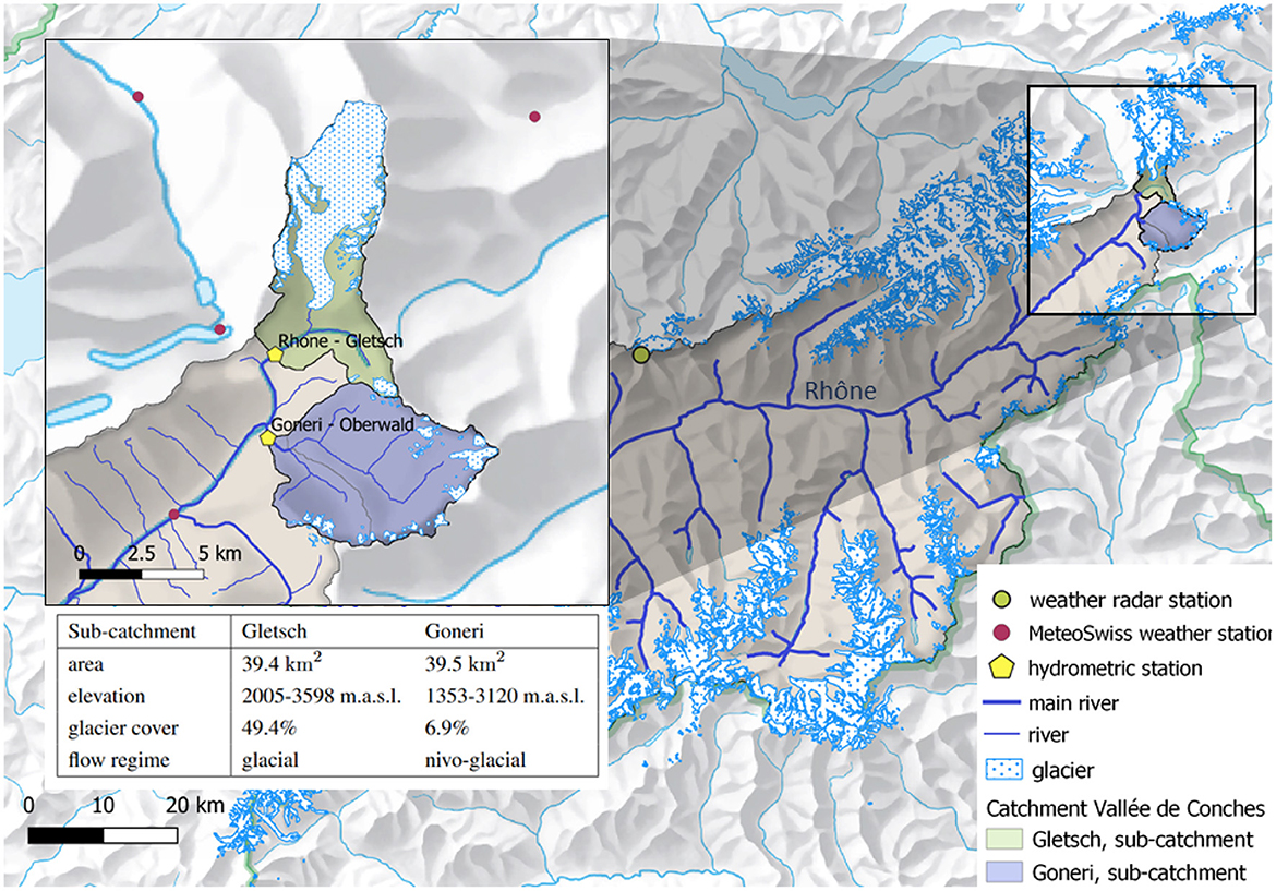
Figure 1. Studied catchment Goms Valley in the canton of Valais, Switzerland. Separation in sub-catchments and associated measurement stations for meteorological and hydrological observations.
2.2. Available observation data
2.2.1. Meteorological forcing data
The Swiss Federal Office of Meteorology and Climatology MeteoSwiss provides historical reanalysis data and real-time observations of precipitation (mm h-1), air temperature (°C) and incoming shortwave radiation (W m-2) for all of Switzerland. Air temperature and radiation are point observations from ground-based weather stations distributed throughout Switzerland. Since 2005, precipitation is available as the gridded product CombiPrecip of 1 km resolution combining radar and rain-gauge observations (Federal Office of Meteorology and Climatology MeteoSwiss, 2014). Before 2005, precipitation is available only from rain gauges.
2.2.2. River flow observations
Observations of river flow discharge (m3 s-1) at the two measurement stations Gletsch and Goneri are operated by the Swiss Federal Office for the Environment FOEN (Federal Office for the Environment FOEN, 2017). The observation history since 1990 was provided by CREALP for this study.
Figure 2 depicts both the mean annual flow and the flow duration curve for the studied period 1999–2020. The observed annual flow patterns can be characterized as nivo-glacial for the station Goneri, and glacial for Gletsch. For both stations, peak flows are reached during the melt season in (late) summer, showing diurnal cyclic patterns due to sub-daily variations of glacier and snow melt induced by variations in air temperature and solar radiation (find a flow example showing the diurnal melting cycles in Figure 9 in the Supplementary material). At both locations, flood events of different magnitudes have been recorded over the considered time period (1999–2020). They often occur at the end of summer on a weak snowpack and high baseflow. Intensive precipitation events can then lead to direct runoff and sometimes mobilize snow melt, producing extreme discharge values.
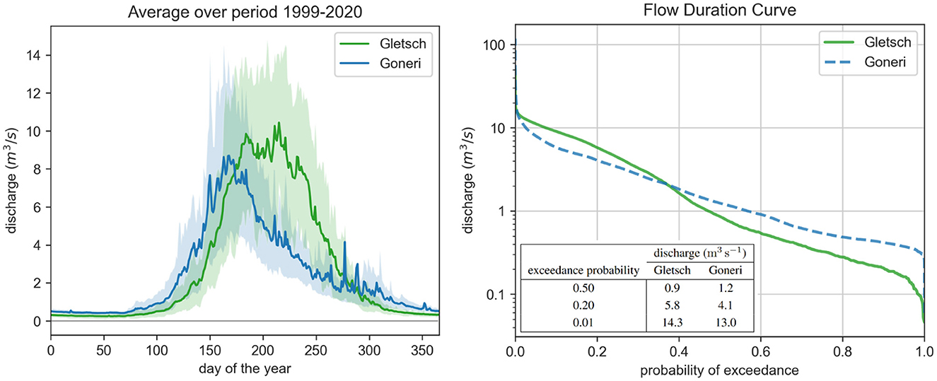
Figure 2. Left: Annual flow measured at the two hydrometric stations Gletsch and Goneri averaged over the studied period from 1999 to 2020. Drawn confidence bands represent the 10% to 90% quantiles. Right: Flow duration curve of the observed discharge at the two hydrometric stations Gletsch and Goneri from 1999 to 2020, depicting the probability of exceedance of a certain discharge value and a table with some key values.
2.3. Data pre-processing
We consider the following meteorological forcing variables at hourly frequency: air temperature, precipitation and incoming shortwave radiation. The forcing data is aggregated in two steps, first on elevation bands, each spanning 400 m of altitude, to account for the large spread in elevation of the alpine catchment. Temperature and radiation observations at the nearest weather stations have been interpolated via inverse distance-weighting, and precipitation has been extracted directly from the CombiPrecip gridded product and integrated over each zone. Subsequently, the resulting elevation band-separated data is aggregated a second time into two zones, a glacier-covered zone and a non-glacial zone, by using the glacier cover extent from swissTLM3D (Federal Office of Topography swisstopo, 2013) in its 2013 version. Glacier-covered areas show different reactions to meteorological forcings due to altered energy and mass flows in the icepack (Hock and Jansson, 2005). The separation will allow the model to learn those different reactions. For better comparison, we assume a constant glacier cover extent as done in the process-based model MINERVE. We highlight that a dynamic glacier cover separation of the inputs would be advised to represent seasonal dynamics and account for shrinking glaciers as observed in the Swiss Alps (Rounce et al., 2023).
The final model inputs are then the three meteorological forcings, once for the glacier-covered zone and once for the non-glacial zone. This specific two-step aggregation scheme was selected in order to keep the number of input variables constant, while still accounting for structural differences between glacier-covered and open terrain.
Previous river discharge is an additional highly informative variable to estimate current and future discharges due to its strong auto-correlation. In some experiments, detailed in Section 3.3, we introduce it in the tested models as an additional input variable. Since the empirical distributions of the discharge at both stations are highly skewed towards small values, we use the natural log-transform of the discharge to focus on changes in magnitudes of flow rate.
3. Methods
This section describes the process-based MINERVE model (Section 3.1) and the data-driven LSTM network architecture we used (Section 3.2). The last two Sections 3.3 and 3.4 describe the experimental setup and evaluation metrics, respectively.
3.1. Process-based model: MINERVE
MINERVE (Hernández et al., 2020) is a process-based rainfall-runoff model developed by CREALP. The MINERVE model performs rainfall-runoff calculations based on a semi-distributed concept and downstream propagation of discharges. Find a simplified description of semi-distributed models and a comparison to other model types in Sitterson et al. (2018). Each element of the model represents a portion of the terrain (i.e., subbasins of the catchment) and models different hydrological processes such as snowmelt, glacier melt, surface and underground flow, etc. These hydrological elements are then linked together in a network of junctions and rivers to simulate runoff processes. MINERVE has been calibrated specifically for the study area and is the state-of-the-art in the studied region used by local authorities to estimate and forecast river discharge.
The model inputs are meteorological variables, i.e., temperature, precipitation and radiation, aggregated on elevation bands as described in Section 2.3. The data is processed by an HBVS (Hydrologiska Byråns Vattenbalansavdelning Valais) module - HBV (Bergström, 1976) adapted by CREALP. Snow and glacier melt are represented by a glacier snow model (GSM) with a Seasonal Degree-day, inspired by Hamdi et al. (2005) and Schaefli et al. (2005). The outflows of the sub-modules are then combined using a transport function to simulate the resulting river flow at the exit of a sub-catchment. In operation mode, previous discharge observations are assimilated to correct the current system states. In this study, we compare to the non-assimilated simulations, which do not use observed discharge as model input, but only exogenous variables.
3.2. Long short-term memory network (LSTM)
This section details the LSTM architecture used in this work and further describes the objective functions, used for training the models. We first introduce the standard LSTM architecture used for the prediction of single values from a generic input sequence in Section 3.2.1 and then extend single prediction to multi-step forecasting with LSTM models. The loss function used for single-step prediction and the loss function for multistep prediction is described in Section 3.2.2. The last sections 3.2.3 and 3.2.4 then briefly describe the implementation details and parameter and hyperparameter optimization process.
3.2.1. Model architecture
The core of the LSTM, as developed by Hochreiter and Schmidhuber (1997), consists of a recurrent cell that is applied iteratively at every observation xt of a sequence (x1, …, xt, …, xT) of T observations as depicted by Figure 3. Two internal memory vectors are updated by several internal gates at each time step: the cell state ct corresponds to the system's long-term memory, and the hidden state ht represents the short-term memory.
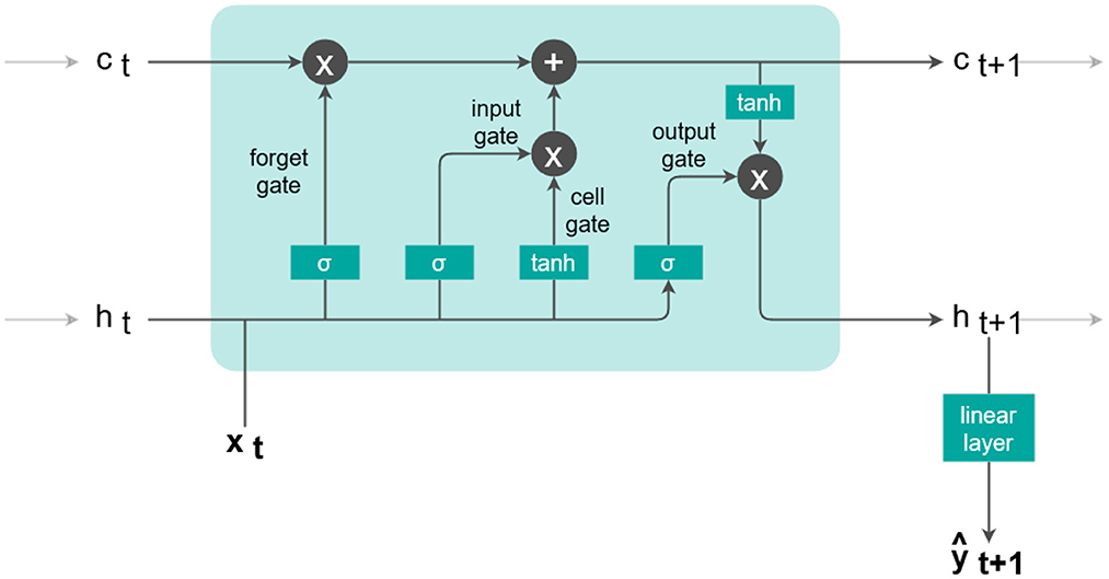
Figure 3. Internal gate structure of an LSTM cell and additional linear output layer.
The four different gates within the LSTM cell update the memory states using a combination of new inputs and previous cell states. They each act like a single layer of nh neurons with weights, bias and an activation function, nh being the chosen hidden size. As a first step, the forget gate
regulates at each time t how much of the information stored in ct is deleted in the long-term memory vector. The input is a vector of d input variables at time t. In each gate, the two weight matrices and and the bias contain randomly initialized parameters and are updated during the training process. The activation function σ represents the sigmoid function; it adds non-linearity to the model and scales the gate output between 0 and 1.The combination of the input gate
and the cell gate
control the new input information written to the long-term memory. Finally, the long-term cell memory state is updated
by deletion of parts in previous cell memory and input of new information. The output gate
then combines new inputs xt and the previous hidden state ht. This gate is modulated by the updated long-term memory ct+1 of Equation (4) to produce the updated hidden state
We use a final linear output layer
to map the hidden state ht+1 of the LSTM cell to a single output of estimated discharge ŷt+1 using the weight parameters Vl and bl.
The overall LSTM model can be abstracted to
where we denote the index exo to indicate that only exogenous variables (meteorological forcings) are inputs to the model (see Figure 4, first setup). We can modify this model to the auto-regressive ar setting
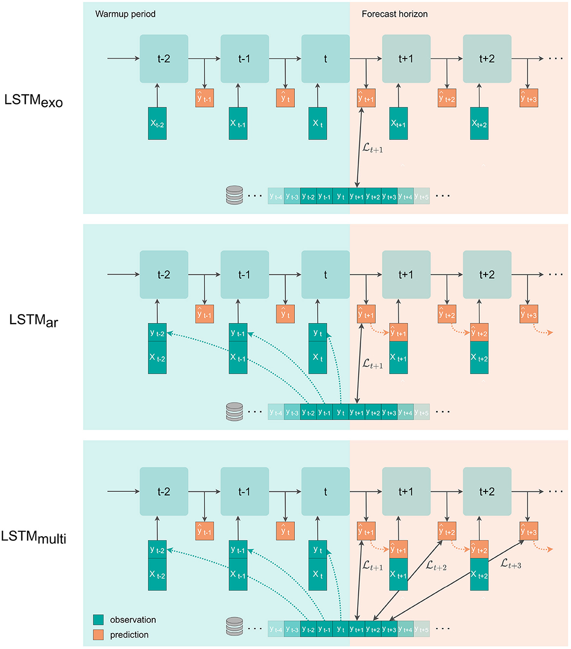
Figure 4. The three setups for multistep-ahead prediction with a single layer LSTM. xt is the vector of meteorological observations (precipitation, temperature, radiation), and yt is the natural logarithm of river discharge at time t. Note that the depicted loss function is applied to the back-transformed discharge values. From Top to Bottom: The LSTMexo setup uses only meteorological input variables and is trained with a loss on the first predicted value. The LSTMar setup uses meteorological inputs plus the discharge signal, which is replaced by the model prediction in the forecast window, and is trained with a single-step loss. The LSTMmulti setup is equal to the setup of LSTMar but is trained using a multistep loss evaluated on the entire forecast window with uniform weights.
by concatenating past flow observations y to the exogenous input vector x, which we denote as (x, y)t for each time point t. Including past discharge observations in the list of input variables allows for utilizing the auto-correlation of the signal in an auto-regressive fashion.
So far, in the auto-regressive setting, we have considered a single-step prediction at t+1, where all input variables (x, y)t are observations. To extend the prediction to multistep-ahead forecasting, we can use the estimated discharge predictions ŷt+1,ŷt+2, … as inputs for the next prediction step (see Figure 4, second setup). This recursive forecasting based on previously estimated discharges can be repeated for an unlimited number of steps. However, we expect forecast performance to drop as prediction errors are propagated with every iteration.
3.2.2. Loss function single-step and multi-step
We can train the model (i.e., optimizing weights and biases of the LSTM cell and linear layer) for single-step prediction by minimizing a loss function between the predicted output ŷi,t+1 and the measured discharge yi,t+1 of a sample i in a dataset of size N. Here, we use the mean squared error over N samples as a loss function to penalize large absolute errors.
For multi-step forecasting in the auto-regressive approach, we can extend the loss function as the average of the sample mean squared errors over the entire predicted sequence of length T (see Figure 4, third setup). In our case, we consider T = 72h.
3.2.3. Hydrological implementation
To ensure that modeled discharge is strictly positive, we predict hourly values of logarithmic discharge in this study. Modeling discharge in magnitudes further allows for covering the high variability in flow observed at the studied locations. In a post-processing step, the predictions are back-transformed using an exponential function. The loss function is still calculated on normal, back-transformed values to prioritize accuracy on high discharge values. In its logarithmic version, the empirical distributions of the discharge have two modes for both stations Gletsch and Goneri. These correspond to low and high flow situations, as shown in Figure 10 in the Supplementary material. The modes are naturally separated by a critical discharge of 1.82 m3 s-1, which we use to evaluate model performance separately for low and high flow later in the experimental Section 4.
We consider two different input feature sets consisting of 6 or 7 input features: In the exogenous variables (exo) setting, we use meteorological forcing variables for both the glacier-covered (g) and non-glacial (ng) zone as described in Section 2.3: Pg, Png, Tg, Tng, Radg and Radng. In the auto-regressive (ar) setting, we additionally use logQ as model input. All variables are used at hourly frequency and are standardized by empirical mean and standard deviation over the training period prior to model input.
When predicting multiple steps, logQ observations are replaced by the model predictions as detailed in Section 3.2.1. For exogenous variables, we always use meteorological observations and not forecasts to focus on the prediction error caused by the LSTM setup. The used meteorological forcings are thus only associated with their measurement error, and additional error caused by the meteorological forecast is not considered.
We use data from 1999 to 2020, which we split into a pre-train, train, validation and test partition in chronological order. We use the last 2 × 15 000 h (~2 × 1.7 years) of data for validation and test/evaluation partitions. In a preliminary analysis, we tested the influence of the length of the test set on model performance evaluation and determined 15 000 h to be the test set length where error metrices stablize and performance evaluation becomes statistically representative. The remaining years are used for training as follows: the LSTMs are first pre-trained on data from the period 1999–2005 (52 500 h) to obtain good parameter initializations. We decided not to include this period in the main training since precipitation data was retrieved from a different source (see Section 2.2.1). Subsequently, the initialized models are trained on the remaining 101 400 h (~11.6 years) of main training data from 2005-2016.
Samples are extracted from the training set as segments consisting of a warmup period (365 days) and the forecasted sequence (one to 72 h). The segments overlap in the warmup period to obtain one sample per time step.
3.2.4. Parameter and hyperparameter optimization
The parameters of the LSTM are determined during training by minimizing the respective loss function - Equation (11) or Equation (12) - on the training set using stochastic gradient descent (SGD). The hyperparameters of the SGD controlling this training process are optimized for the validation set using a grid search of the following values: learning rate (step size of the gradient descent {0.001, 0.01, 0.05, 0.1, 0.3, 0.5}) and weight decay (a regularization to avoid overfitting {10−2, 10−3, 10−4, 10−5}). The optimal learning rate and weight decay were found to be different for the three LSTM models trained in this study and are listed in Table 3 in the Supplementary material. The batch size (number of samples in memory during one iteration) was set to 512 beforehand, according to the available VRAM.
We chose a lightweight model structure with a single LSTM layer and minimal model size to accelerate the calibration process. The hidden size nh (corresponding to the size of cell state and hidden state, tested values: {1, 2, 4, 8, 16, 32}) determined the number of model parameters and was optimized in a preliminary study. A hidden size that is too small will result in an oversimplified model, which is not able to represent all the hydrological relationships. If it is chosen too large, unnecessary degrees of freedom are awarded through a large number of model weights and biases, slowing down the calibration process. The determined hidden size of 4 - leading to a number of 197 model parameters for LSTMexo and 213 for LSTMar and LSTMmulti - was fixed for all LSTM variations, to keep the model size consistent.
During training, the selected initial learning rate as reported in Table 3 in the Supplementary material was gradually reduced until convergence, a common practice in neural network training. For every LSTM setup we developed an ensemble of ten models with different random parameter initializations to represent the inherent error of the model. The final model performance is then evaluated on the test set as the mean over each ensemble.
3.3. Experimental setup
Figure 5 summarizes the adopted workflow including feature selection, pre-processing and the three analyses of the trained models. Throughout this work, we consider a forecast horizon of 72 h for the LSTMs and compare their performance to the process-based model MINERVE. The forecast window of 72 hours was selected according to the quality expected degradation due to accumulating errors in the estimated flow that is used as input to the LSTM model for the next time step. Note that in the present setup, we only use meteorological observations and not forecasts, as outlined in Section 3.2.3. For every tested LSTM setup, we developed an ensemble consisting of ten individual models, described in Section 3.2.4, and evaluate the mean performance over the ensemble.

Figure 5. Adopted workflow, starting with feature selection and pre-processing, followed by the training of different LSTM setups (ensemble of 10 models each) and testing of general performance, feature importance analysis, and the robustness to a change of domain.
3.3.1. Multistep-ahead prediction
In this set of experiments, we compare three different LSTM model setups for forecasting of river discharge in the sub-catchment Gletsch as depicted by Figure 4: (a) using only meteorological/exogenous variables to forecast discharge (LSTMexo), (b) exogenous and discharge as input with a single-step loss (LSTMar) and (c) exogenous and discharge as input with a multistep loss (LSTMmulti). Through comparison of LSTMexo and LSTMar we examine the importance of adding discharge inputs for the prediction. When discharge is included in the feature set, its observations are no longer available after the point of forecast and are replaced by the predicted value. We thus expect an increasing model error with progressing forecast and test whether extending the single-step loss function on the entire 72-h window, as adopted by LSTMmulti, can reduce this effect.
We compare all LSTM setups with the process-based model MINERVE, which uses the same set of input variables as LSTMexo. To test whether the LSTMs that receive past discharge as input variable are learning more than just copying the discharge values, we compare against a simplistic baseline model, which copies the last observed discharge for the entire forecast window.
The multistep-ahead predictions will reveal the best LSTM setup according to the selected criteria defined in Section 3.4, which we then select for the subsequent experiments.
3.3.2. Permutation feature importance
After determining the best LSTM setup in the previous experiment, LSTMmulti, we test whether meaningful relationships between the input variables were learned by the model. We use permutation feature importances to rank the input features by relevance (Breiman, 2001; Fisher et al., 2019). This method consists of shuffling the time-series of a feature in the test set and evaluating the trained model on this time-series. The procedure is repeated for each feature, recording the mean drop in performance over ten different random permutations.
Permutation feature importance is a model agnostic method and thus applicable to any model type and is further independent of the actual feature distribution. It however evaluates each feature separately, whereas as significant correlation and interdependence between features might exist and thus only allows to get a general idea of the relevance of the input variables. Other more sophisticated methods, such as Shapley Additive Explanation (SHAP) or Local Interpretable Model-Agnostic Explanations (LIME) (Holzinger et al., 2022), take variable interrelation into account and can provide additional insight about the directional influence of a variable. In contrast to these methods, permutation feature importance can be easily implemented for any model with few lines of code, making it an accessible explainability tool for an initial assessment of variable importance.
3.3.3. Application on other sub-catchment
We continue again with the best-performing LSTM setup and aim to test one of the main limitations of data-driven models: they are often limited to the training domain and perform poorly when transfering to new domains (Devia et al., 2015). Testing out-of-domain allows to assess whether reasonable physical relationships have been learned [question (i)]. With this experiment, we further evaluate if fine-tuning the trained model on the new domain over a few epochs can boost the performance [question (ii)]. If successful, this would allow to use the pre-trained model and transfer it to a catchment with limited amount of observation data, e.g., if a gauging station was only recently installed in the area of interest.
To address these questions we test and compare the performance of three differently trained LSTMmulti on the neighboring sub-catchment Goneri. We chose Goneri as test location because of its comparable surface area and climatic similarity to Gletsch. Both catchments are located in the same valley, thus, we expect reasonable performance of a hydrological model that has learned the correct basic relationships. To answer question (i) we apply the model, which we previously trained on the Gletsch sub-catchment, directly on the neighboring sub-catchment Goneri. We denote this model LSTMGletsch. This test will inform about the robustness of the model, i.e., whether it overfits to the specifics of the sub-catchment. For question (ii), we compare two models: LSTMGoneri, trained only on data from Goneri, and LSTMGletsch+Goneri, the trained Gletsch model finetuned on data from Goneri over ten training epochs. The three LSTM models are compared to the local calibrated version of the process-based model MINERVE similar to the previous experiment.
3.4. Evaluation metrics
The prediction performance of the developed models is assessed by visual inspection of the predicted hydrographs and through several metrics common for hydrological model evaluation. The target river discharge is separated into the low flow (Q ≤ 1.82 m3 s-1) and the high flow (Q>1.82 m3 s-1) regime and evaluation is carried out separately on these regimes. These two flow regimes were determined through visual inspection of the log-histogram of discharge which is naturally separated in two clusters (see Section 3.2.3 and Figure 10 in the Supplementary material). To test the model performance for extreme events, under-represented in the training set, two example flood events were selected from the validation and test period: September 4-7, 2016, with an estimated return period of 29 years, and October 2-5, 2020, with an estimated return period of 2 years [estimated return periods from Federal Office for the Environment FOEN (2021)].
The following metrics have been chosen for the performance evaluation, the respective equations are listed in Supplementary material 7.3. We use the Root-mean-square error (RMSE) as an absolute error metric in the unit of discharge, a perfect RMSE would be 0 m3 s-1. The volumetric efficiency (VE) (Criss and Winston, 2008) is a performance score and lies in the range of -∞ to 1. It measures the volume bias as the integral under the discharge curve. A perfect model would have a VE of 1, negative values indicate that the model prediction error is larger than the observed discharge value. The VE and RMSE can be used to evaluate short sequences and are thus selected as primary performance criteria for multi-step prediction.
The Nash Sutcliffe efficiency (NSE) (Nash and Sutcliffe, 1970) scores the simulation performance of the model compared to using the empirical average as a predictor. An NSE of 0 describes a model as good as the mean, a perfect model would have an NSE of 1. Similarly, the Kling-Gupta efficiency (KGE) (Gupta et al., 2009) describes the shape of the curve and combines several measures of bias, variance and correlation coefficient into one score. A perfect model would have a KGE of 1. The NSE and KGE are used for continuous time series and thus not suitable for evaluating short sequences, such as the 72 h of this study. We therefore used these metrics only to evaluate continuous time series of single-step predictions, which are listed in Table 4 in the Supplementary material.
4. Results
4.1. Multistep-ahead prediction
This section compares the LSTM in different setups - regarding input features and loss function - with the process-based model MINERVE and a baseline copying the last flow value. We compare the models in three flow regimes. In Section 4.1.1, we consider low and high-flow situations, while Section 4.1.2 compares models qualitatively on flood events in the evaluation area.
4.1.1. Low and high flow regimes
Figure 6 depicts the results of the multistep-ahead forecasts of the different tested LSTM setups. Each line consists of the mean performance over the ten ensemble members, with a standard deviation drawn as a confidence band. We show how performance develops along the forecast steps with RMSE as a metric. The LSTM is compared to the process-based model MINERVE, as well as a baseline copying the last observed value over the entire 72-h forecast horizon. The larger the RMSE, the larger the absolute error of the prediction. In Table 1 we further list RMSE and VE values of some key forecast horizons.
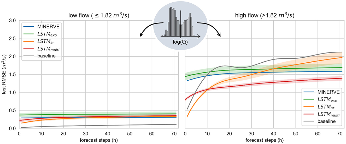
Figure 6. Test results of multistep-ahead prediction of river discharge in Gletsch by the LSTM models, the process-based model MINERVE and the baseline (copies the last available discharge observation at t = 0h). Reported is the root mean squared error (RMSE) for different forecast horizons, separated into low flow (Left) and high flow regime (Right). For the LSTM, the depicted line represents the mean over the developed ensembles consisting of ten models each, with a confidence band of one standard deviation.
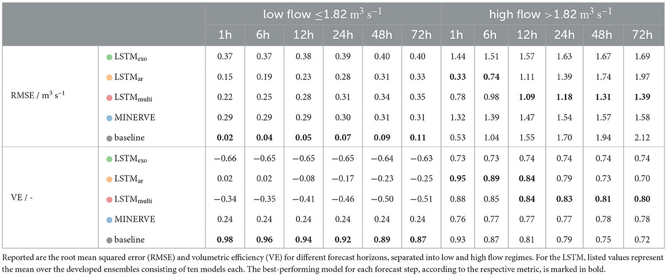
Table 1. Test results of multistep-ahead prediction of river discharge in Gletsch by the developed LSTM models, the process-based model MINERVE and the baseline (copies the last available discharge observation at t=0h).
A significant difference is observed between predictions of low flow and high flow regimes, which were distinguished using the empirical histogram of the logarithmically transformed discharge as described in Section 2.3. Absolute errors on low flow are very small, stable over time and do not exceed 0.4 m3 s-1 for all models (compared to average flow values observed at this station in Figure 2). Judging by the RMSE, all LSTMs perform similarly to MINERVE when considering the spread of the respective LSTM ensembles. We note that the baseline shows the lowest RMSE error with 0.11 m3 s-1 after 72 hours, suggesting that a simplistic auto-regressive model is sufficient to describe the low flow regime. Furthermore, the volumetric efficiency of all LSTM is negative or close to zero, which indicates that the LSTM prediction error is larger than the river flow value itself.
In the high flow regime, clear differences between the models are visible. The prediction accuracy of the LSTMexo, which uses only meteorological forcings as input, as well as of the process-based model MINERVE stays constant over the entire forecast window as depicted by the green and blue line in Figure 6, respectively. MINERVE is thereby slightly more accurate in terms of both RMSE and VE.
Adding past discharge values to the input vector, as implemented in the LSTMar (orange line in Figure 6), results in a significantly lower error than MINERVE for the first few forecast steps. To verify whether the increased performance for the initial forecast hours can be traced back to the auto-correlation of the discharge signal, we compare against the simplistic baseline, which copies the last available discharge observation to the entire forecast horizon. Since the baseline and LSTMar pattern are very similar, we conclude that the LSTMar very likely attributes the largest importance to the discharge input feature. This hypothesis is further supported by the steep increase in RMSE that exceeds the LSTMexo after 40 hours. If the relationships between meteorological forcings and output discharge were correctly learned by the model, prediction error would level out around the LSTMexo instead of exceeding it after a few steps.
Adapting the loss function for multistep prediction resolves this issue, supporting our initial hypothesis. The LSTMmulti has an initial performance that lies in between LSTMexo and LSTMar and deteriorates only minorly with progressing forecast. For forecast horizons over 12 hours, the LSTMmulti is the best of the compared models. This is confirmed in Table 1, showing that the VE of LSTMmulti is larger than the models with only meteorological inputs over the entire forecast horizon. Additionally, a lower spread within the model ensemble compared to the other trained LSTM is observed in Figure 6.
4.1.2. Performance for flood events
We tested all the models for multistep prediction of two selected flood events with a lead time of about 24 h. Figure 7 depicts the predictions of the three LSTM models, compared to MINERVE and the baseline. The drawn lines of the LSTM are the ensemble median with a confidence band ranging from the 10% to 90% quantile.
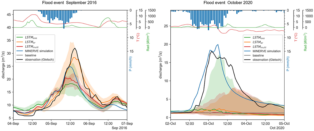
Figure 7. Test results of multistep-ahead prediction of two example flood events (Left: 2016 event; Right: 2020 event) in Gletsch by the LSTM models, the process-based model MINERVE and the baseline (copies the last available discharge observation at t = 0h); and meteorological variables observed during the event averaged over the entire sub-catchment. For the LSTM, the depicted line represents the median over the developed ensembles consisting of ten models, with a confidence band of the 10-90% quantile. Note that MINERVE was recalibrated to fit the October 2020 flood event particularly well.
The observed LSTM forecast performance is different for the two events. While the timing of the flood peak in the 2016 event is captured well by all LSTM setups, the peak discharge is underestimated by the LSTMexo and LSTMmulti. Prediction performance is here comparable to the process-based model MINERVE. In 2020, only LSTMexo managed to represent the dynamics of the flood event, while the other LSTM largely underestimated the peak. MINERVE performed here significantly better and reached the full peak height. It is, however, crucial to note that the MINERVE version used in this study was recalibrated to fit this specific flood event particularly well, which can alter the interpretation of this event. The baseline predicts a constant value for the entire forecast horizon and is not suited for predicting specific events.
The different performance of the models on the flood events can be explained by the underlying mechanisms being fundamentally different between the events. The 2016 event was a precipitation driven flood: at the end of summer the snowpack is fully melted and a large precipitation event is transformed directly to a runoff-peak. Both MINERVE and LSTM thus manage to capture this regular flood event reasonably well. The 2020 event, in contrast, presented more complex dynamics. As shown in Figure 7, recorded temperatures were only slightly above zero when precipitation started to intensify. During the subsequent translation into runoff and rise of the discharge peak, temperatures drop around zero, switching between solid and liquid precipitation. Note that the temperature profile shown in Figure 7 is the average over the entire catchment, i.e., temperatures were below zero in the high-altitude and above zero in the low-altitude section of the catchment. It could thus be expected that the models perform badly on this event with such exceptional conditions.
Next to the performance difference between different events, we observe a performance difference between the tested LSTM setups. For instance in the 2016 event, LSTMar occurs to be the best predictor. While this observation can be drawn for this single event, no model consistently outperforms the others in the studied anomalies. We attribute this inconsistency to the rare nature of these events, that are not captured sufficiently in the training data. We could hypothesize performances during the 2016 event to be linked to the duration of the precipitation, to the magnitude of the event, or to the fact that LSTMar uses logQ as input, yet no general conclusion can be drawn on a single event. Further studies specifically designed for anomalous floods are necessary to assess these properties of models more thoroughly, which we reserve for future studies.
Generally, the prediction of flood events is a specifically challenging task as precipitation magnitudes are at the high end of the historically observed conditions. In addition, floods are often triggered by specific mechanisms, such as rain on snow, that are not yet sufficiently understood to represent them in a model. Data-driven models, which learn from correlation and distributions of the data, are thus expected to perform poorly on out-of-sample conditions. Nevertheless, we showed with this experiment that at least one of the tested LSTM setups is able to represent the general dynamics of the flood events similarly well to the process-based model MINERVE. The setup with agreeable performance to MINERVE is hereby different for the two events: LSTMar is best in September 2016, LSTMexo is best for the flood of October 2020.
4.2. Feature importance
In the previous experiment, we identified LSTMmulti as the best-performing setup within the tested LSTMs. To justify its performance and disclose the relationships learned by the LSTM we calculate permutation feature importances for the LSTMmulti setup. This model agnostic method defines feature importance by the drop in performance (or increase in test error) when the observed time-series of a feature is replaced by a series of random values drawn from the feature's empirical distribution. We calculate accordingly the increase in test RMSE for 1h-ahead predictions on the test period. Only high flow conditions are evaluated, since the variation of the model simulations during low flow conditions was minimal and we thus expect a smaller impact when omitting a feature. The process is repeated ten times per feature for statistical stability and we report the mean over the permutations in Table 2. A bigger increase in test error indicates a stronger focus of the model on the values of this feature.
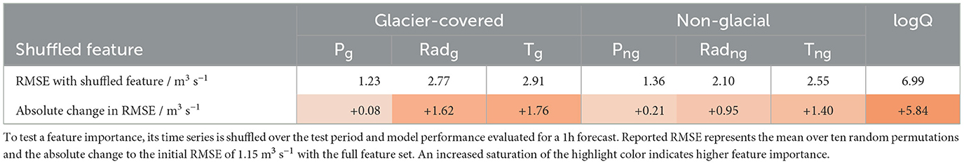
Table 2. Permutation feature importances for LSTMmulti evaluated on high flow conditions (>1.82 m3 s-1) in the test set.
The auto-regressive input feature logQ shows the strongest increase in RMSE of +5.84 m3 s-1 after shuffling its values. It was expected that the discharge is a strong predictor since it is highly auto-correlated over the forecast window, which can be concluded from the strong performance of the simple baseline during the first forecast hours. Next important features are air temperature Tg and incoming solar radiation Radg over the glacier-covered area. This coincides with the strong influence of the glacier on the local hydrology in Gletsch (observed, e.g., by the diurnal cycles shown in Table 2). The LSTM seems to capture this relationship and thus reacts predominantly to temperature and radiation over the glacier - the main drivers of glacial melt.
Both precipitation features, over the glacier-covered and open terrain, exhibit the smallest change in RMSE. While the applied method allows a certain look inside the black-box model, it is limited by the empirical distribution of the feature. Precipitation is zero most of the times and rarely rises to an important level. Shuffling the values will thus only seldom lead to significantly deviant values, biasing the analysis and falsely indicating a small importance of the precipitation feature. Even though this feature fell under the radar of permutation feature importances, the good performance of the LSTM on the flood events shows that the LSTM does indeed react to precipitation.
A way to overcome this draw-back of the permutation feature importances would be to apply other explainability methods such as Shapley Additive Explanation (SHAP), Local Interpretable Model-Agnostic Explanations (LIME) or GRADient Class Activation Mapping (GRAD-CAM) as suggested by Chakraborty et al. (2021) and Machlev et al. (2022). SHAP, for instance, is based on game theory and takes inter-dependence of predictor variables into account, and GRAD-CAM is a deep learning-specific approach allowing to unveil local feature contributions for specific events. While these post-hoc methods are computationally complex and costly (Holzinger et al., 2022), they could provide a more accurate ranking of global and local variable importance and are worth exploring in future studies.
4.3. Extension to other sub-catchments
We selected the best LSTM setup, LSTMmulti, according to the findings of the multistep evaluation in Section 4.1.1 and applied it to the neighboring sub-catchment Goneri in different training setups as introduced in Section 3.3. Figure 8 summarizes the multistep prediction results of the three compared training setups. The LSTM setups compare similarly under high flow and low flow conditions. We thus limit the description of this experiment's results to high flow conditions and refer to the Supplementary material for the low flow results (Figure 11).
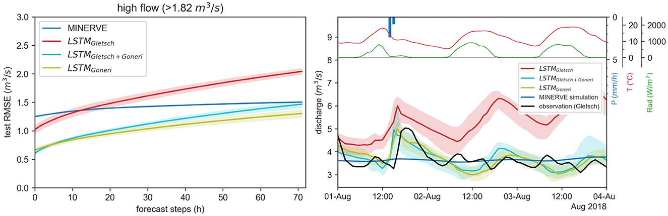
Figure 8. Left: Test results of multistep-ahead prediction of river discharge in Goneri by the process-based model MINERVE and the developed LSTM models: trained only on Gletsch, trained first on Gletsch then fine-tuned on Goneri, trained only on Goneri. Reported is the root mean squared error (RMSE) for different forecast horizons under high flow conditions. The depicted line represents the mean over the developed ensembles, with a confidence band of one standard deviation. Right: Prediction example of hourly discharge of the developed LSTM models and MINERVE for the sub-catchment Goneri. For the LSTM, the depicted line represents the median over the developed ensembles consisting of ten models, with a confidence band of the 10–90% quantile.
The LSTMGletsch is the LSTMmulti tested directly on Goneri data without further finetuning. It reaches high accuracy on the new area, with an RMSE of 1.1–2.1 m3 s-1 when forecasting 1 or 72 steps, respectively. Additional finetuning on the new sub-catchment (LSTMGletsch+Goneri) can, however, improve the predictions to a significant extent and reduce the RMSE at 72 h to 1.5 m3 s-1. A comparison with LSTMGoneri, the LSTM model tuned from zero on the Goneri catchment, reveals that the high performance can be primarily attributed to training on data from the considered area, as both models perform similarly well. Starting with a model that was trained on the neighboring area does not contribute to the performance, however, decreases the training time needed for the new area. This result from the analysis of the RMSE is confirmed by inspection of a flow example depicted in the right panel of Figure 8. All LSTM models capture well the dynamics of the hydrograph and react to incoming precipitation with an increase in discharge, while the process-based model MINERVE seems to predict a constant discharge for this timeframe. LSTMGletsch hereby over-estimates the flow and reacts more strongly to temperature and radiation.
5. Discussion
The results of this work demonstrate that data-driven LSTM models that ingest the previous flow rate together with meteorological variables achieve better accuracy than the established conceptual bucket model MINERVE in the glacially-influenced Goms Valley in Switzerland. We focused in this study on high-flow situations with flow rates above 1.82 m3 s-1, which are most challenging to model accurately to provide knowledge for applications like hydroelectric power estimation (Ogliari et al., 2020) or flood risk assessment (Alfieri et al., 2013). Under low flow conditions with inconsiderable flow variability, a simplistic model that copies the last available discharge value (termed “baseline”) showed to be sufficient in terms of prediction error. We also evaluated the models on two distinct flood events, but found that the prediction performance of all tested models was mixed for these flood events, which we attribute to the challenges of modeling these rare events that include new hydrodynamic mechanisms that are under-represented in the training set. Depending on the event, some LSTM setups could capture the flood peak well, and some under-estimated peak discharge comparable to the process-based model.
In the high flow regime, we found the LSTM variants that use past discharge as model input next to meteorological variables, i.e., LSTMmulti and LSTMar, most effective, as they can harness the auto-correlation of the discharge signal. Concretely, the best LSTM variant for longer term forecasting of ≥12 h, i.e., LSTMmulti, predicted headwater discharge with an RMSE of 1.39 m3 s-1 for a 72 h forecast window compared to MINERVE with 1.58 m3 s-1. In short-term forecast <12 h, the LSTMar model predicted the flow most accurately followed by LSTMmulti and MINERVE. This is due to the different loss function used between LSTMar and LSTMmulti, where an accurate long-term forecast is explicitly encouraged in LSTMmulti by including all 72 prediction steps in the loss function at equal weight. In contrast, LSTMar is optimized to accurately predict only the next single step, which naturally leads to more accurate short-term predictions, as we see in the experiments (Figure 6). We would like to emphasize that these results were achieved with a lightweight model with only 213 trainable parameters, which is highly parameter-efficient and makes the prediction with tested LSTMs computationally efficient next to ensuring that the LSTM is less prone to overfitting.
The results were verified by transferring the model to the neighboring location, the Goneri sub-catchment (Section 4.3), and by a feature importance analysis (Section 4.2) that re-emphasizes the importance of ingesting previous flow in the model, but also reveals that the model preferentially uses temperature and radiation measurements above the glacier cover for its predictions. While the adopted permutation approach to measure feature importances is a fast and simple way to verify that reasonable physical relationships were learned by the model, it is limited to provide a first impression. Other more elaborate methods need to be applied to obtain more accurate and detailed measures of global and local interpretability with correlated input variables (Chakraborty et al., 2021). For instance SHAP and LIME (Holzinger et al., 2022) are two model agnostic strategies allowing to take variable interactions into account and calculate directional feature contributions. A common strategy specific for deep learning models is the analysis of gradients, which enabled to reveal dynamic feature contributions for LSTM in the study of Kratzert et al. (2019). Gradient analysis provides exact measures of local dependencies, as compared to approximate values obtained through LIME, and could potentially help in improving the understanding of the glacial hydrological processes in the studied catchment.
In general, we observed that separating the analysis of the developed LSTM into low and high flow regimes was crucial, as different models achieved best results depending on the flow situation. While high flow conditions, occurring during the melt season in spring and summer, are modeled well by the LSTM, relative errors are large during low flow in the accumulation season, where the baseline models achieved best results. We attribute this to runoff-generating processes being different in winter than in summer, making it challenging for the model to learn to represent these different mechanisms equally well. Another important observation is that the LSTM was particularly sensitive to parameter initialization. We addressed this by training multiple LSTM models and making ensemble predictions. This ensemble spread, especially visible during the analysis of the two flood events, emphasizes the importance of developing a model ensemble to cover model-inherent uncertainty, as highlighted by Kratzert et al. (2021).
Modeling in glacier-influenced catchments can be especially challenging due to the highly dynamic processes present in the alpine environment, which are often not yet fully understood (Tiel et al., 2020). In contrast to process-based models, DL models infer processes from correlations in the input data and do not need a precise description of the processes. In particular, LSTM are time-aware DL models that still resemble the general structure of process-based models, and contain memory states that are able to learn storage processes such as snow accumulation. LSTM are thus suitable as hydrological models and could be established for many catchments in a much shorter time than with process-based models, where model structure and parameters need to be adapted manually when moving to other catchments.
A general limit of the setup, as presented in this study, is that input data was aggregated on the glacier and non-glacier-covered zones with a fixed surface area, whereas climate change scenarios report a shift in glacier extent and snow-covered area for Switzerland. To ease this constraint, meteorological inputs could be aggregated using a dynamic delineation of the glacier-covered area based on real-time satellite images, scaling the variables by the respective surface area of each zone. A further limitation comes from the lightweight character of the developed LSTM.
While the light-weight model architecture with few trainable parameters has several practical and computational benefits, it may not have the internal capacity to learn very complex behaviors. Given related work with substantially larger deep learning models (Kratzert et al., 2018; Feng et al., 2020), we hypothesize that our light-weight LSTM may not be optimal in this particular configuration when used as a large regional model and utilizing public datasets such as CAMELS (Addor et al., 2017), or the soon available Swiss version [CAMELS-CH (Höge et al., 2023)]. Still, we did not observe better performance on our evaluated catchments when increasing the model capacity in this work. Nevertheless, our comparison of input features and loss functions should be transferable directly to larger regional models and our explicit feature importance and transferability studies provide a general insight into the applicability of data-driven LSTM models in Switzerland and for glacial catchments in general.
6. Conclusion
Operational flood and water resource management require accurate short-term predictions of river discharge by hydrological models. With this work, we showed that the previously demonstrated power of data-driven deep learning models for hydrological modeling can be extended to alpine catchments in operational frameworks. Besides the good performance, deep learning models can be set up faster, while being more flexible than their process-based counterparts. The flexibility with respect to the choice of input data allowed us, for instance, to integrate past discharge observations to supersede complex data-assimilation techniques.
We believe that adaptive, fast reactive models as the one we propose are truly needed: under changing climate conditions, the shift in flow regimes that is starting to be observed further raises the need for models that can follow new distribution with limited calibration time and that can be transferred between catchments without full re-calibration. We hope that this work will contribute to the further application of data-driven deep learning models for forecasting runoff in alpine environments in synergy with current conceptual models.
Data availability statement
The used data is available upon request to the corresponding author. Requests to access these datasets should be directed to Y29yaW5uYS5mcmFua0BhbHVtbmkuZXBmbC5jaA==.
Author contributions
DT, JF-S, MR, and CF contributed to the conception and design of the study. CF performed the main model development and analysis and wrote the first draft of the manuscript. JF-S performed data preprocessing. MR wrote sections of the manuscript. All authors contributed to manuscript revision, read, and approved the submitted version.
Acknowledgments
This project is based on the Master Thesis of CF, which was hosted jointly by the Centre de recherche sur l'environnement alpin CREALP and the Environmental Computational Science and Earth Observation Laboratory at EPFL. The authors kindly thank CREALP for providing the observation data used in this study and gratefully acknowledge the financial assistance provided by EPFL for publishing of this article.
Conflict of interest
The authors declare that the research was conducted in the absence of any commercial or financial relationships that could be construed as a potential conflict of interest.
Publisher's note
All claims expressed in this article are solely those of the authors and do not necessarily represent those of their affiliated organizations, or those of the publisher, the editors and the reviewers. Any product that may be evaluated in this article, or claim that may be made by its manufacturer, is not guaranteed or endorsed by the publisher.
Supplementary material
The Supplementary Material for this article can be found online at: https://www.frontiersin.org/articles/10.3389/frwa.2023.1126310/full#supplementary-material
References
Addor, N., Newman, A. J., Mizukami, N., and Clark, M. P. (2017). The CAMELS data set: catchment attributes and meteorology for large-sample studies. Hydrol. Earth Syst. Sci. 21, 5293–5313. doi: 10.5194/hess-21-5293-2017
Alfieri, L., Burek, P., Dutra, E., Krzeminski, B., Muraro, D., Thielen, J., et al. (2013). Glofas-global ensemble streamflow forecasting and flood early warning. Hydrol. Earth Syst. Sci. 17, 1161–1175. doi: 10.5194/hess-17-1161-2013
Anderson, S., and Radić, V. (2022). Interpreting deep machine learning for streamflow modeling across glacial, nival, and pluvial regimes in southwestern Canada. Front. Water. 4, 934709. doi: 10.3389/frwa.2022.934709
Bergström, S. (1976). Development and application of a conceptual runoff model for scandinavian catchments. SMHI, Norrköping. Reports RHO, 7.
Campolo, M., Soldati, A., and Andreussi, P. (1999). Forecasting river flow rate during low-flow periods using neural networks. Water Resour. Res. 35, 3547–3552. doi: 10.1029/1999WR900205
Chakraborty, D., Başağaoğlu, H., and Winterle, J. (2021). Interpretable vs. noninterpretable machine learning models for data-driven hydro-climatological process modeling. Expert Syst. Appl. 170:114498. doi: 10.1016/j.eswa.2020.114498
Criss, R. E., and Winston, W. E. (2008). Do nash values have value? Discussion and alternate proposals. Hydrol. Proc. 22, 2723–2725. doi: 10.1002/hyp.7072
Crook, D. S. (2001). The historical impacts of hydroelectric power development on traditional mountain irrigation in the valais, switzerland. Mt. Res. Dev. 21, 46–53.
de la Fuente, A., Meruane, V., and Meruane, C. (2019). Hydrological early warning system based on a deep learning runoff model coupled with a meteorological forecast. Water. 11, 1808. doi: 10.3390/w11091808
Devia, G. K., Ganasri, B. P., and Dwarakish, G. S. (2015). A review on hydrological models. Aquatic Procedia. 4, 1001–1007. doi: 10.1016/j.aqpro.2015.02.126
Federal Office for the Environment (2017). Hydrological Data and Forecasts. Available online at: http://hydrodaten.admin.ch (accessed October 10, 2022).
Federal Office for the Environment (2021). Flood Statistics. Available online at: https://www.bafu.admin.ch/bafu/en/home/topics/water/state/data/flood-statistics.html (accessed October 10, 2022).
Federal Office of Meteorology Climatology MeteoSwiss (2014). Documentation of MeteoSwiss Grid-Data Products - Hourly Precipitation Estimation Through Raingauge-Radar: Combiprecip. Available online at: https://www.meteoswiss.admin.ch/services-and-publications/service/weather-and-climate-products.html (accessed October 10, 2022).
Federal Office of Topography swisstopo (2013). swisstlm3d. Available online at: https://www.swisstopo.admin.ch/en/geodata/landscape/tlm3d.html (accessed February 20, 2023).
Feng, D., Fang, K., and Shen, C. (2020). Enhancing streamflow forecast and extracting insights using long-short term memory networks with data integration at continental scales. Water Resour. Res. 56, 9. doi: 10.1029/2019WR026793
Fisher, A., Rudin, C., and Dominici, F. (2019). All models are wrong, but many are useful: Learning a variable's importance by studying an entire class of prediction models simultaneously. J. Mach. Learn. Res. 20, 1–81. doi: 10.48550/arXiv.1801.01489
Gupta, H. V., Kling, H., Yilmaz, K. K., and Martinez, G. F. (2009). Decomposition of the mean squared error and NSE performance criteria: Implications for improving hydrological modelling. J. Hydrol. 377, 80–91. doi: 10.1016/j.jhydrol.2009.08.003
Hamdi, Y., Hingray, B., and Musy, A. (2005). Un modèle de prévision hydro-météorologique pour les crues du rhône supérieur en suisse. Technical report. Baden: Schweizerischer Wasserwirtschaftsverband SWV. doi: 10.5169/seals-941778
Hegg, C., McArdell, B. W., and Badoux, A. (2006). One hundred years of mountain hydrology in switzerland by the wsl. Hydrol. Proc. 20, 371–376. doi: 10.1002/hyp.6055
Hernández, J. G. (2011). “Flood management in a complex river basin with a real-time decision support system based on hydrological?,” in Communication 48 du Laboratoire de Constructions Hydrauliques, ed E. A. Schleiss (Lausanne: Ecole Polytechnique Fédérale de Lausanne EPFL). doi: 10.5075/epfl-thesis-5093
Hernández, J. G., Claude, A., Arquiola, J. P., Roquier, B., and Boillat, J.-L. (2014). “Integrated flood forecasting and management system in a complex catchment area in theAlps' implementation of the MINERVE project in the Canton of Valais,” in Swiss Competences in River Engineering and Restoration, Schleiss, A., Speerli, J., Pfammatter, R. (eds.). Boca Raton, FL: CRC Press. doi: 10.1201/b17134-12
Hernández, J. G., Foehn, A., Fluixá-Sanmartín, J., Roquier, B., Brauchli, T., Arquiola, J. P., et al. (2020). RS MINERVE – Technical Manual. Sion: Centre de recherche sur l'environnement alpin (CREALP) and HydroCosmos SA.
Hochreiter, S., and Schmidhuber, J. (1997). Long short-term memory. Neural Comput. 9, 1735–1780. doi: 10.1162/neco.1997.9.8.1735
Hock, R., and Jansson, P. (2005). Modeling glacier hydrology. J. Glaciol. 66, 1–11. doi: 10.1002/0470848944.hsa176
Höge, M., Kauzlaric, M., Siber, R., Schönenberger, U., Horton, P., Schwanbeck, J., et al. (2023). Catchment attributes and hydro-meteorological time series for large-sample studies across hydrologic Switzerland (CAMELS-CH) (0.1) [Data set]. Zenodo. doi: 10.5281/zenodo.7784633
Höge, M., Scheidegger, A., Baity-Jesi, M., Albert, C., and Fenicia, F. (2022). Improving hydrologic models for predictions and process understanding using neural ODEs. Hydrol. Earth Syst. Sci. 26, 5085–5102. doi: 10.5194/hess-26-5085-2022
Holzinger, A., Saranti, A., Molnar, C., Biecek, P., and Samek, W. (2022). “Explainable AI methods - a brief overview,” in xxAI - Beyond Explainable AI. Midtown Manhattan, New York City: Springer International Publishing. p. 13–38. doi: 10.1007/978-3-031-04083-2_2
Hsu, K.-,l., Gupta, H. V., Gao, X., Sorooshian, S., and Imam, B. (2002). Self-organizing linear output map (solo): an artificial neural network suitable for hydrologic modeling and analysis. Water Resour. Res. 38, 38–31. doi: 10.1029/2001WR000795
Kao, I.-F., Zhou, Y., Chang, L.-C., and Chang, F.-J. (2020). Exploring a long short-term memory based Encoder-Decoder framework for multi-step-ahead flood forecasting. J. Hydrol. 583, 124631. doi: 10.1016/j.jhydrol.2020.124631
Kratzert, F., Herrnegger, M., Klotz, D., Hochreiter, S., and Klambauer, G. (2019). “NeuralHydrology, interpreting LSTMs in hydrology,” in Explainable AI: Interpreting, Explaining and Visualizing Deep Learning, Lecture Notes in Computer Science, Samek, W., Montavon, G., Vedaldi, A., Hansen, L. K., and Müller, K.-R. (eds). Midtown Manhattan, New York City: Springer International Publishing. p. 347–362. doi: 10.1007/978-3-030-28954-6_19
Kratzert, F., Klotz, D., Brenner, C., Schulz, K., and Herrnegger, M. (2018). Rainfall-runoff modelling using long short-term memory (lstm) networks. Hydrol. Earth Syst. Sci. 22, 6005–6022. doi: 10.5194/hess-22-6005-2018
Kratzert, F., Klotz, D., Hochreiter, S., and Nearing, G. S. (2021). A note on leveraging synergy in multiple meteorological data sets with deep learning for rainfall–runoff modeling. Hydrol. Earth Syst. Sci. 25, 2685–2703. doi: 10.5194/hess-25-2685-2021
Lees, T., Reece, S., Kratzert, F., Klotz, D., Gauch, M., De Bruijn, J., et al. (2022). Hydrological concept formation inside long short-term memory (LSTM) networks. Hydrol. Earth Syst. Sci. 26, 3079–3101. doi: 10.5194/hess-26-3079-2022
Machlev, R., Heistrene, L., Perl, M., Levy, K., Belikov, J., Mannor, S., et al. (2022). Explainable artificial intelligence (XAI) techniques for energy and power systems: Review, challenges and opportunities. Energy and AI. 9, 100169. doi: 10.1016/j.egyai.2022.100169
Mohammadi, B., Safari, M. J. S., and Vazifehkhah, S. (2022). Ihacres, gr4j and misd-based multi conceptual-machine learning approach for rainfall-runoff modeling. Sci. Rep. 12, 12096. doi: 10.1038/s41598-022-16215-1
Nash, J., and Sutcliffe, J. (1970). River flow forecasting through conceptual models part i —a discussion of principles. J. Hydrol. 10, 282–290. doi: 10.1016/0022-1694(70)90255-6
Ogliari, E., Nespoli, A., Mussetta, M., Pretto, S., Zimbardo, A., Bonfanti, N., et al. (2020). A hybrid method for the run-of-the-river hydroelectric power plant energy forecast: hype hydrological model and neural network. Forecasting. 2, 410–428. doi: 10.3390/forecast2040022
Rounce, D. R., Hock, R., Maussion, F., Hugonnet, R., Kochtitzky, W., Huss, M., et al. (2023). Global glacier change in the 21st century: every increase in temperature matters. Science. 379, 78–83. doi: 10.1126/science.abo1324
Schaefli, B., Hingray, B., Niggli, M., and Musy, A. (2005). A conceptual glacio-hydrological model for high mountainous catchments. Hydrol. Earth Syst. Sci. 9, 95–109. doi: 10.5194/hess-9-95-2005
Shen, C., Chen, X., and Laloy, E. (2021). Editorial: Broadening the use of machine learning in hydrology. Hydrol. Earth Syst. Sci. 3, 681023. doi: 10.3389/frwa.2021.681023
Sit, M., Demiray, B. Z., Xiang, Z., Ewing, G. J., Sermet, Y., and Demir, I. (2020). A comprehensive review of deep learning applications in hydrology and water resources. Water Sci. Technol. 82, 2635–2670. doi: 10.2166/wst.2020.369
Sitterson, J., Knightes, C., Parmar, R., Wolfe, K., Avant, B., and Muche, M. (2018). “An overview of rainfall-runoff model types,” in International Congress on Environmental Modelling and Software (Washington, DC: U.S. Environmental Protection Agency). p. 41.
Keywords: hydrological model, LSTM, short-term forecast, machine learning, alpine, streamflow, glacier, rainfall-runoff
Citation: Frank C, Rußwurm M, Fluixa-Sanmartin J and Tuia D (2023) Short-term runoff forecasting in an alpine catchment with a long short-term memory neural network. Front. Water 5:1126310. doi: 10.3389/frwa.2023.1126310
Received: 17 December 2022; Accepted: 29 March 2023;
Published: 17 April 2023.
Edited by:
Hossein Shafizadeh-Moghadam, Tarbiat Modares University, IranReviewed by:
K. S. Kasiviswanathan, Indian Institute of Technology Roorkee, IndiaHakan Basagaoglu, Edwards Aquifer Authority, United States
Copyright © 2023 Frank, Rußwurm, Fluixa-Sanmartin and Tuia. This is an open-access article distributed under the terms of the Creative Commons Attribution License (CC BY). The use, distribution or reproduction in other forums is permitted, provided the original author(s) and the copyright owner(s) are credited and that the original publication in this journal is cited, in accordance with accepted academic practice. No use, distribution or reproduction is permitted which does not comply with these terms.
*Correspondence: Corinna Frank, Y29yaW5uYS5mcmFua0BhbHVtbmkuZXBmbC5jaA==