The contribution of remote sensing and input feature selection for groundwater level prediction using LSTM neural networks in the Oum Er-Rbia Basin, Morocco

The planning and management of groundwater in the absence of in situ climate data is a delicate task, particularly in arid regions where this resource is crucial for drinking water supplies and irrigation. Here the motivation is to evaluate the role of remote sensing data and Input feature selection method in the Long Short Term Memory (LSTM) neural network for predicting groundwater levels of five wells located in different hydrogeological contexts across the Oum Er-Rbia Basin (OER) in Morocco: irrigated plain, floodplain and low plateau area. As input descriptive variable, four remote sensing variables were used: the Integrated Multi-satellite Retrievals (IMERGE) Global Precipitation Measurement (GPM) precipitation, Moderate resolution Imaging Spectroradiometer (MODIS) normalized difference vegetation index (NDVI), MODIS land surface temperature (LST), and MODIS evapotranspiration. Three LSTM models were developed, rigorously analyzed and compared. The LSTM-XGB-GS model, was optimized using the GridsearchCV method, and uses a single remote sensing variable identified by the input feature selection method XGBoost. Another optimized LSTM model was also constructed, but uses the four remote sensing variables as input (LSTM-GS). Additionally, a standalone LSTM model was established and also incorporating the four variables as inputs. Scatter plots, violin plots, Taylor diagram and three evaluation indices were used to verify the performance of the three models. The overall result showed that the LSTM-XGB-GS model was the most successful, consistently outperforming both the LSTM-GS model and the standalone LSTM model. Its remarkable accuracy is reflected in high R² values (0.95 to 0.99 during training, 0.72 to 0.99 during testing) and the lowest RMSE values (0.03 to 0.68 m during training, 0.02 to 0.58 m during testing) and MAE values (0.02 to 0.66 m during training, 0.02 to 0.58 m during testing). The LSTM-XGB-GS model reveals how hydrodynamics, climate, and land-use influence groundwater predictions, emphasizing correlations like irrigated land-temperature link and floodplain-NDVI-evapotranspiration interaction for improved predictions. Finally, this study demonstrates the great support that remote sensing data can provide for groundwater prediction using ANN models in conditions where in situ data are lacking.

1. Introduction

Groundwater is of crucial importance as an essential source of drinking water, providing around half of the world's drinking water supply. It also plays a vital role in supporting agriculture, meeting almost 40% of irrigation needs, contributing to food security and the sustainability of water resources (Dumont, 2021; Elshall et al., 2022). This importance is even greater in the context of North Africa, particularly in countries such as Morocco, where the challenges posed by arid and semi-arid environments amplify its value. Despite its undeniable importance, the current state of monitoring and warning systems for this resource is very worrying. The scarcity of effective mechanisms for monitoring and responding to the state of groundwater highlights the urgent need to improve our approach to resource management in these regions (Hamed et al., 2018; Sherif et al., 2023). Within hydrogeology, the conventional techniques for observing groundwater, which encompass wells and piezometers used to gauge groundwater levels and outline its development, are put into practice. However, in many African basins, the monitoring and assessment of groundwater resources is inadequate, lacking the comprehensive coverage needed to understand the complex dynamics of its environment (World Meteorological Organization, 2020). In certain instances, the piezometric networks currently in operation suffer from dysfunctionality, riddled with gaps that result in data lags spanning several months, and occasionally, even years. This temporal lag critically impedes the capacity for real-time evaluation of groundwater quantitative and qualitative changes, particularly during drought periods. In response, modeling and forecasting of groundwater quantity and quality variables have become essential to support water resources management and strategy (Cui et al., 2022).

Artificial neural networks (ANNs) have proven to be very effective tools for predicting groundwater variables, mainly due to their remarkable ability to capture complex and subtle patterns in the data (Rajaee et al., 2019; Zhu et al., 2022). By integrating historical and heterogeneous data, ANNs can apprehend non-linear patterns and variations that are challenging to discern using traditional conceptual and physical-based methods. Their capacity to generalize from training data empowers them to generate accurate forecasts, even amidst changing conditions, all while not necessarily requiring a complete comprehension of the underlying hydrogeological processes (Rajaee et al., 2019). Moreover, ANNs can be adjusted and refined over time, continuously enhancing their forecasting performance. They can also be integrated with optimization techniques to swiftly calibrate models, thereby expediting the decision-making process in groundwater management. ANNs were first used in groundwater monitoring in the late 1990s and early 2000s, and it has since become a well-established area of research (Maier et al., 2010; Rajaee et al., 2019; Tao et al., 2022). Several studies demonstrated that ANN models such as Multilayer Perceptron (MLP) Neural Network, Input Delay Neural Network (IDNN) and Recurrent Neural Network (RNN) are able to predict groundwater level up to several months, even years in advance (Coulibaly et al., 2001; Daliakopoulos et al., 2005; Nayak et al., 2006; Nourani et al., 2008, 2022; Trichakis et al., 2011; Taormina et al., 2012; Moghaddam et al., 2019; Sahu et al., 2020; Kouadri et al., 2022). Moreover, ANNs can be used to model spatial variations in the water table if observations from a well network are available (Sharafati et al., 2020; Malakar et al., 2021). ANNs can also be used to improve the performance of spatiotemporal groundwater predictions for aquifers, either as a replacement for or in conjunction with existing physical models (Nourani et al., 2011; Taormina et al., 2012; Wunsch et al., 2021).

In this study, we focus on the application of the Long Short-Term Memory (LSTM) model to predict time series data related to groundwater levels. LSTM is an improved architecture of the Recurrent Neural Network (RNN) (Hochreiter and Schmidhuber, 1997). Designed for sequential data, the LSTM model suits the prediction of groundwater variables with temporal dependencies. Its key advantage lies in retaining information from the time series' beginning, enabling it to capture long-term patterns relevant for groundwater variables influenced by climate, cyclical phenomena, and extended temporal scales. LSTM architecture employs memory gates to control the flow of information, allowing it to capture seasonal trends, irregular fluctuations, and gradual shifts in groundwater levels (Shin et al., 2020; Van Houdt et al., 2020; Kim et al., 2021). Thanks to its aptitude for retaining information from prior periods, the LSTM model excels in predicting time series characterized by intricate oscillations and non-linear trends. In modeling complex groundwater behavior, the LSTM's adeptness at handling time-based patterns and extensive dependencies makes it a crucial tool for accurate forecasting (Zhang et al., 2018; Vu et al., 2021; Khan et al., 2023). The LSTM model has several hybrid and optimization forms, such as the LSTM-Weighted Mean of Vectors Optimizer (INFO), LSTM- Ant Lion Optimizer (ALO) and LSTM- Ensemble Empirical Mode Decomposition (EEMD), which proved effective in predicting hydrological variables such as water temperature and streamflow (Yuan et al., 2018; Huang et al., 2023; Ikram et al., 2023). By merging the strengths of LSTMs with pertinent historical and environmental data, this approach presents a robust tool for precision prediction and proficient management of groundwater levels.

Predicting groundwater level using complex neural network architectures like LSTM model requires an access to a comprehensive database that covers a complex chronicle of fluctuations in groundwater levels, alongside an array of pertinent explanatory factors (Rajaee et al., 2019). Of particular significance are climatic series, notably including variables such as precipitation patterns and temperature records (Ghose et al., 2018; Kouziokas et al., 2018; Zhang et al., 2018). Furthermore, hydrological time series, such as river discharge, contribute to the complex interaction of water movements between surface and subsurface environments (Mohanty et al., 2015; Sahu et al., 2020). Equally vital are parameters like evapotranspiration rates, which quantify the transfer of moisture from the Earth's surface into the atmosphere through processes like plant transpiration and soil evaporation (Ghose et al., 2018; Zhang et al., 2018). Additionally, the inclusion of pumping rates, serves as a critical determinant of groundwater availability and variation (Trichakis et al., 2011; Mohanty et al., 2015). However, a notable constraint and challenge in the application of ANNs for groundwater prediction lies in the availability and reliability of these input data. Reliable in situ measurements of climatic variables such as precipitation, temperature and evapotranspiration are often hampered by measurement irregularities and the presence of erroneous data (Kuglitsch et al., 2009; Toreti et al., 2012; Ledesma and Futter, 2017). Constraints related to terrain accessibility, changes in measurement conditions, relocation of weather stations, changes in land use, adoption of new instruments and changes in observation times all contribute to the potential unreliability of collected data.

These challenges are particularly pronounced in regions where the monitoring infrastructure is inadequate, notably in Africa, where only one-eighth of the minimum density of weather stations is available (World Meteorological Organization, 2020). The scarcity of these crucial observation points within these regions, directly affects the potential accuracy and robustness of ANNs when applied to groundwater prediction models. Although ANNs excel at capturing complex relationships within data, their effectiveness relies heavily on the quality and quantity of data fed into the model (Sahu et al., 2020).

In such context of increasing in situ data scarcity, climate and Earth observation data derived from remote sensing have offered researchers a great opportunity to study and analyse hydro-geo-dynamic processes in a new way (Li et al., 2022; Zhang and Zhang, 2022). Remote sensing technology, with its ability to collect large amounts of climate and Earth observation data with considerable and complex heterogeneity on dynamic Earth systems such as soil, water and vegetation, and complemented by the ability of satellites to repeatedly cover large areas through regular visits, has found great application in modeling hydrological processes (Becker, 2006; Chawla et al., 2020; Adams et al., 2022; Li et al., 2022). However, the convergence of remotely sensed data and artificial intelligence for groundwater level prediction only became apparent in late 2019 and early 2020 (Bhanja et al., 2019; Sharafati et al., 2020; Malakar et al., 2021; Sureshkumar et al., 2022; Stateczny et al., 2023; Zhang et al., 2023). These recent studies have highlighted the potential of integrating remote sensing data as input parameters in ANN models. Yet, there are still several aspects of this approach that need to be studied in more detail. Indeed, groundwater aquifers are characterized by a wide diversity and heterogeneity of geo-environmental features such as depth, unconfined or confined aquifer conditions, and different types of usage like irrigation and water supply. These factors can significantly condition and influence the use of remote sensing data as descriptive variables to model their groundwater variables (Adams et al., 2022). On the other hand, remote sensing data also encompass various characteristics that can impact their ability to explain variations in groundwater variables, such as spatial and temporal resolution and data presented in various forms (Adams et al., 2022).

Advances in remote sensing technologies, the deployment of numerous satellites and the development of data storage systems have led to the accumulation of an enormous volume of climate and environmental data (Sahu et al., 2020). In the light of this, a crucial question arises as to the optimum approach: should we exploit a diverse range of explanatory factors or rely on a single variable that most effectively reveals variations in groundwater levels? The choice between these approaches adds another layer of complexity to the application of remote sensing data for groundwater prediction through ANN models. While employing multiple variables might capture a broader spectrum of influencing factors and interactions, it can also introduce challenges related to data dimensionality, potential multicollinearity, and increased computational complexity (Dormann et al., 2013; Anh et al., 2023). On the other hand, focusing on a single variable that has the strongest correlation with groundwater levels might simplify the modeling process but could oversimplify the hydrodynamic mechanism within the aquifer system. Currently, there is no general consensus in the literature regarding the optimal choice of variables. The number and selection of variables depend on the specific objectives and characteristics of the study case (Rajaee et al., 2019).

In order to shed light on these issues and provide valuable insights, this study aims two main objectives: firstly, to assess the effectiveness of incorporating remote sensing data into LSTM models for predicting groundwater levels; and secondly, to investigate the ramifications of input feature selection on prediction accuracy. Additionally, the research this study seeks to extend its examination by considering predictions across diverse hydrodynamic and land cover-land use conditions. To achieve this, three LSTM models for groundwater level prediction were developed, rigorously analyzed and compared. The first model, named LSTM-XGB-GS, was optimized using the GridsearchCV method, which is a hyperparameter optimization technique (Chen et al., 2023). This model uses a single variable identified by the XGBoost method, an input feature selection technique (Zhang B. et al., 2022; Jiang et al., 2023). This selected variable is considered the most effective in explaining variations in groundwater level among four remotely sensed variables: GPM precipitation, MODIS NDVI, MODIS evapotranspiration, and MODIS LST. Another optimized LSTM model was also constructed, but uses the four variables as input (LSTM-GS). Additionally, a standalone LSTM model was established and also incorporating the four variables as inputs. These models were employed to predict groundwater levels in five wells located within significantly diverse geo-environmental and land use conditions, including an irrigated zone, an alluvial plain, and a confined aquifer in a plateau area, within the Oum Er-Rbia river Basin (OER) in Morocco. The models developed in this study will pave the way for the establishment of a single, global groundwater level prediction model capable of helping water managers to predict groundwater levels in regions characterized by variable hydrogeodynamic conditions and land use.

2. Materials and methods

2.1. Study area

The study area is located in the OER River Basin, in the north-central part of Morocco, between latitudes 31° 00' and 33° 00' North and longitudes 5° 00' and 9° 00' West (Figure 1A). The study area comprises two main regions with very different hydrogeological, land use and relief contexts: the phosphate plateau and the Tadla plain (Figure 1B). The climate in the study area is semi-arid to arid with a continental character. Precipitation is irregularly distributed in time and space within the basin. There is a dry season from May to October and a wet season from November to April. During the dry season the minimum inter-annual monthly rainfall averages are as low as 0.8 mm, however the average maximum is over 72 mm during the winter. From north to south, the increase in altitude is accompanied by an increase in precipitation amount and a decrease in temperature.

FIGURE 1

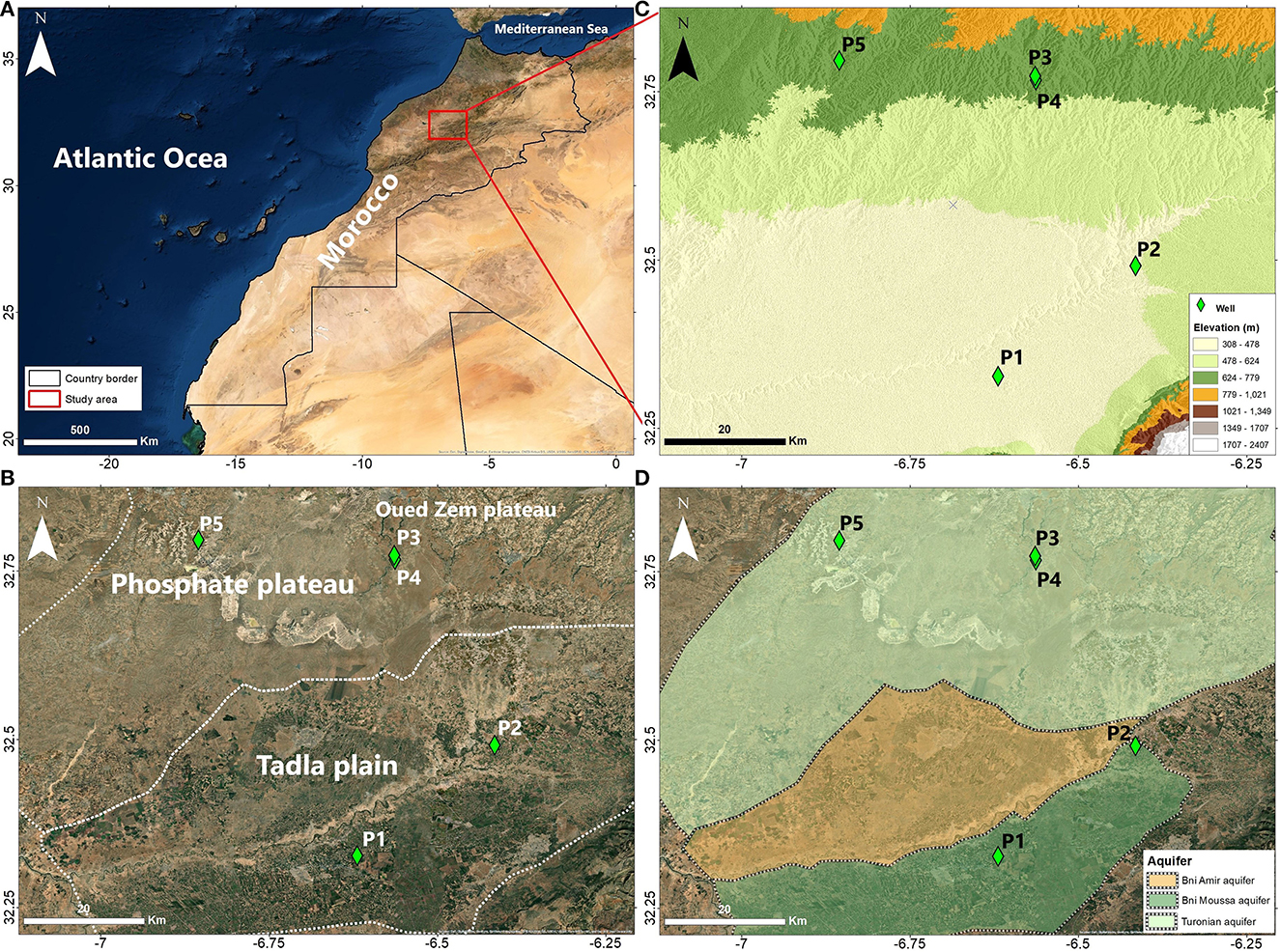
Figure 1. (A) Location of the study area, (B) main geographical areas, (C) altitude variation and (D) the main aquifers in the study area.

In the OER River Basin, groundwater aquifers are subject to constant monitoring, encompassing both qualitative and quantitative variables. This region benefits from a particularly extensive historical groundwater dataset, unlike other parts of Morocco where data is sparse. The comprehensive database available in the OER basin owes its central role as one of Morocco's agricultural hubs (Ouatiki et al., 2019; Khellouk et al., 2021; Lionboui et al., 2021). Five wells are investigated in this study, wells P1 (Figure 2A) and P2 (Figure 2B) are located in the Tadla Plain which is characterized by a generally regular topography at an average altitude of 400 m and a gentle slope toward the west (Figures 1B, C). The Tadla plain is divided by the OER wadi into two hydrogeological zones: the Beni Amir aquifer to the north and the Beni Moussa aquifer to the south, in which the P1 and P2 wells are located (Figure 1D). The water table of the Tadla plain is formed by Villafranchian and Quaternary lacustrine limestone arranged in discontinuous lenses separated by low permeability formations. The agricultural areas in this plain cover 320 000 ha that include 124 000 ha as irrigated areas (Lionboui et al., 2021).

FIGURE 2

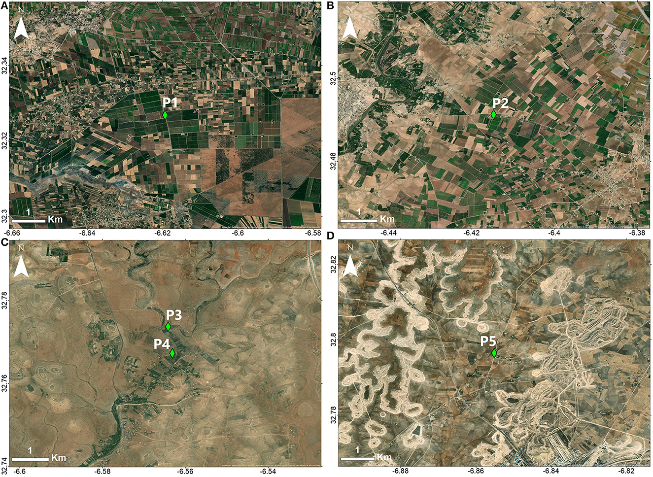
Figure 2. Location of wells (A) P1, (B) P2, (C) P3 and P4, (D) P5.

Wells P3, P4 (Figure 2C) and P5 (Figure 2D) are located in the phosphate plateau (Figure 1B). These wells belong to the Turonian deep water table which is the most important one in the Tadla (Figure 1D), circulating in limestone and dolomitic limestone formations. However, these three wells are located in distinct hydrological contexts. Wells P3 and P4 are located in the floodplain of the Wadi Zem, which dissipates further south into the alluvium without merging with the OER River. Well P5, shows the greatest depth to the water table (average depth = 72 m), is located further north in the center of the phosphate plateau in a semi-arid environment near the phosphate mines (Figure 2D). Table 1 presents the descriptive statistics of groundwater level observed for each well.

TABLE 1

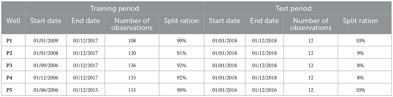
Table 1. Distribution of groundwater level data for training and test periods.

2.2. Datasets

2.2.1. Observed groundwater level records

Monthly groundwater level observations were provided by the Oum Er-Rbia basin agency. The length of the time series of the five wells is not uniform (Figure 3). However, the difference in length is not very high, ranging from 1 to 3 years of difference (Table 1). The time series for each well was divided into training and test periods. The length of the training period varies between wells due to the non-uniformity of the time series, but the length of the test period is constant and has been set as the last year of the time series in each well (Table 1). The decision to assign a single year allows a comprehensive assessment of the model's adaptability to distinct seasonal profiles and facilitates direct comparison of its performance between wells, providing valuable information on its ability to handle variable seasonal fluctuations and data patterns under different hydrodynamic conditions. For neural networks developed for big data processing, this variation in the length of time series is negligible and does not influence model performance between wells (Vu et al., 2021; Wei et al., 2021). Table 2 presents the statistical description of the groundwater level in each well.

FIGURE 3

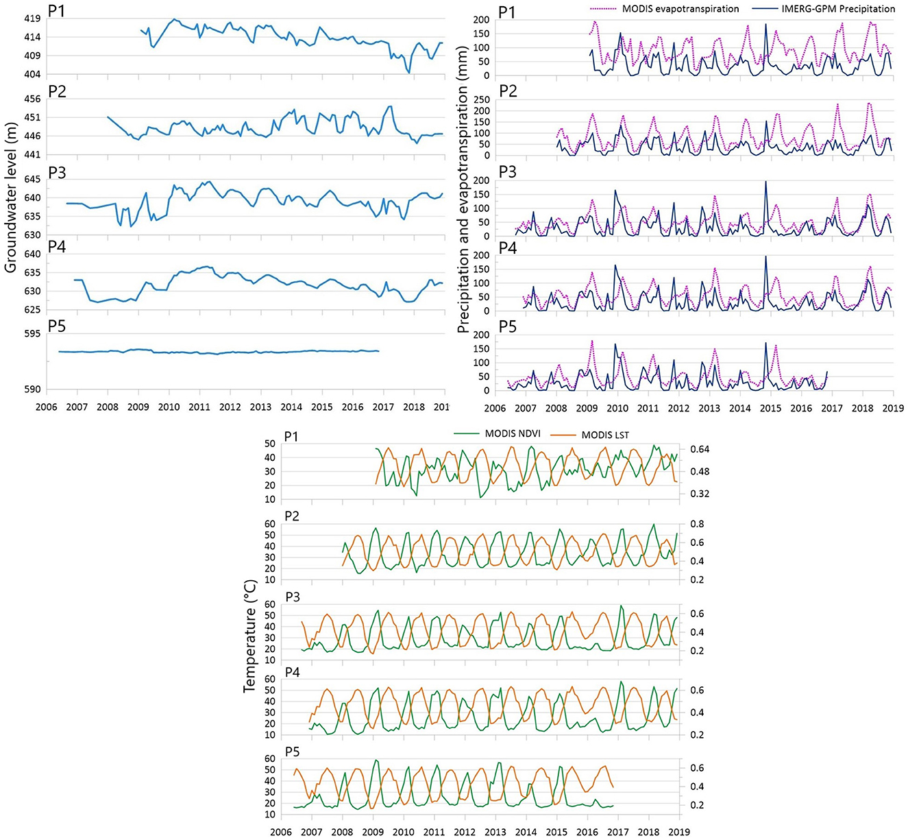
Figure 3. Monthly variation of the observed groundwater level, IMERG-GPM precipitation, MODIS evapotranspiration, MODIS LST and MODIS NDVI of the five studied wells.

TABLE 2

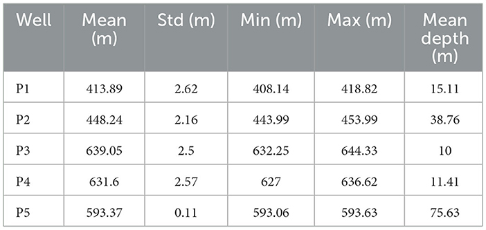
Table 2. Groundwater level description.

2.2.2. Remote sensing data

The groundwater level is influenced by several geo-environmental and climates factors such as precipitation, evapotranspiration, soil moisture, hydrodynamic parameters of the aquifer, pumping and irrigation activities, and aquifer recharge (Rinderer et al., 2016; Iqbal et al., 2020; Band et al., 2021). In this work four remotely sensed variables were used, namely precipitation, land surface temperature, evapotranspiration and normalized difference vegetation index (NDVI). Precipitation, temperature and evapotranspiration are the most frequently used climate variables for forecasting groundwater level (Rajaee et al., 2019; Tao et al., 2022). This is due to their strong influence on groundwater fluctuations and their availability thanks to the several satellite products that provide global coverage with several spatial and temporal resolutions. Furthermore, thanks to its long archives at low and moderate spatial resolutions are available, NDVI has become one of the most widely used remote sensing products for ecosystem analysis, mapping, and land monitoring at regional scales (Azzali and Menenti, 2000; Epting et al., 2005; Fu and Burgher, 2015; Marchetti et al., 2016; Htitiou et al., 2021; Lebrini et al., 2021).

The monthly variation of NDVI at the studied wells was extracted from the NDVI product (MOD13Q1) version 6 of the Terra Moderate Resolution Imaging Spectroradiometer (MODIS), with a spatial resolution of 250 meters and a temporal frequency of 16 days. The temperature variation at each well was determined using the MODIS MYD11A2 product Version 6, which provides an average 8-day per-pixel land surface temperature and emissivity (LST&E) at a spatial resolution of 1 km. Monthly evapotranspiration data are obtained from the MODIS MOD16A2 evapotranspiration product version 6 with a spatial resolution of 500 m and a temporal resolution of 8 days. Monthly precipitation data for each well were obtained from the Integrated Multi-Satellite Retrievals (IMERG) for Global Precipitation Mission (GPM) program with a spatial resolution of 10 km (Huffman et al., 2020). Figure 3 illustrates monthly changes in MODIS LST and NDVI for each well, while Figure 3 represents monthly changes in MODIS evapotranspiration and IMERG-GPM precipitation.

2.3. Data pre-processing

2.3.1. Handling missing data

The database of the wells studied had several missing monthly values scattered throughout the time series. However, it should be noted that these wells were selected from a large network of wells because they do not have more than two successive missing monthly values. Missing values can present many problems in the data set. They can reduce the statistical power of the data, and increase its bias (Kang, 2013). It is therefore necessary to process these missing values in order to maintain the characteristics of the data. In this study, we employ linear interpolation, which performs well in cases of brief missing data, given that consecutive missing data points within the time series do not exceed two observations (Bikše et al., 2023). This method estimates the absent monthly groundwater level by leveraging the values of neighboring months, thus seamlessly integrating the missing data into the groundwater level time series (Huang, 2021).

2.3.2. Feature scaling

Feature scaling is a crucial step in the pre-processing of data for forecasting models. Inputs with high values disproportionately mask the impact of inputs with lower values. The range of predictors should also be matched to the range of the hidden layer transfer function (Cabaneros et al., 2019; Chen et al., 2020). The standardization method has been incorporated into the algorithm of the groundwater level prediction model used in this study. Thus, the input variables are scaled in such a way that they end up having the properties of a standard normal distribution with a mean of zero and a standard deviation of 1. This is done by simply calculating the Z-score of each observation in the data set for each variable, as follows:

$\begin{array}{ll}Z(i)=\frac{Valuei-Std}{Mean}& (1)\end{array}$

Where Z(i) is the normalized value of each observation, Value i is the input value for month (i), Std and Mean are respectively the standard deviation and the average input value of the whole time series.

2.4. Input features selection

Predicting groundwater levels using remote sensing data from several climate variables for several wells with very different dynamics necessitates an understanding of the data that goes into the model. As a result, a variable importance analysis can help us understand the relationship between the descriptive variables and the target variable, and determine which features are not relevant to the model in each well (Sahu et al., 2020; Sharafati et al., 2020; Khaire and Dhanalakshmi, 2022).

Traditionally, important variables are chosen using correlation coefficient analysis, with the selected variables being those with the highest correlations with groundwater levels (Derbela and Nouiri, 2020; Band et al., 2021; El Bilali et al., 2021; Vu et al., 2021). However, strongly correlated input variables can have a negative impact on the performance of a modeling algorithm. When using multiple correlated variables, the effect of collinearity occurs, resulting in unstable and unreliable model results. To avoid this, choosing the best single variable eliminates the need to use multiple variables and their potential interactions, preventing over-learning and allowing the model to generalize better to new, unknown data (Dormann et al., 2013; Anh et al., 2023).

Thus, before building the model, it is critical to examine the correlations between the input variables and the variable to be predicted in order to assess their relationships in a fairly straightforward and descriptive manner. However, it is recommended to use input feature selection techniques, which calculate a score for all input features of a given model that simply represent the importance of each variable (Sahu et al., 2020). A higher score means that the variable will have a greater effect on the model that is used to predict the groundwater level. In this study we used the Extreme Gradient Boosting (XGBoost) method, which constructs boosted trees to obtain the scores of the variables, indicating their importance for the modeling model (Hastie et al., 2009; Breiman et al., 2017; Zheng et al., 2017). The scores provided by XGBoost indicate the usefulness or value of each variable in building the boosted decision trees in the model. The more a variable is used to make key decisions with the decision trees, the higher its relative importance (Friedman, 2002; Zheng et al., 2017). XGBoost counts the importance by “gain”, which is the main reference factor of the variables importance in the tree branches (Hastie et al., 2009; Breiman et al., 2017; Zheng et al., 2017):

$\begin{array}{ll}{\omega }_l^2(T)=\frac{1}{M}{\sum }_{m=1}^M{\tau }_t^2(T_m)& (2)\end{array}$

With T as a decision tree, ω_l importance score for each predictor variable, M is the additive number of trees et ${\tau }_t^2$ is the estimated maximum improvement of the variable in the risk of squared error over that of a constant fit.

2.5. Recurrent neural network model: LSTM

Specifically designed for handling sequential data, the LSTM model is highly suitable for forecasting both qualitative and quantitative groundwater variables, which often exhibit temporal dependencies. One of the main advantages of the LSTM model is its ability to retain information on events that occurred at the start of the time series, even as it processes new data. This feature is crucial for capturing long-term dependencies and patterns present in time series data. This is especially relevant for groundwater variables, as they are influenced by climatic seasonality and other phenomena with return times spanning several years or even longer periods.

The mathematical representation of a RNN is defined by the equation (Hochreiter and Schmidhuber, 1997; Gers et al., 2000):

$\begin{array}{ll}{h}_t=\sigma (b_h+U.X_t+W.h_{t-1})& (3)\end{array}$

$\begin{array}{ll}{y}_t=b_o+(V.h_t)& (4)\end{array}$

Where, h_t is the initial state at time t, h_t−1 is the hidden state of the cell at time t-1, X is the input vector with the sequence, σ and the activation function of TanH, b_h and b_o bias vector, U is the weight (vector) for the hidden layer, V is the weight (vector) for the output layer, W is the same weight vector for different time steps, and y the output vector with the sequence.

The RNN uses the time backpropagation approach, which is a type of gradient descent algorithm that is used to update the weight and minimize errors using a derived chain rule. However, the way the RNN is structured does not allow for effective long-term dependency treatment, as its learning process leads to the vanishing gradients (Hochreiter, 1998). This problem is due to the fact that during the backpropagation the weights are the same for all time steps, as the weight is updated continuously, so that the gradient becomes either too weak or too strong with the updates. One of the solutions to this problem is the use of long-term memory (LSTM) (Graves, 2012). The LSTM was built to avoid the problem of long-term dependencies, by having an additional feature compared to RNNs, which is called memory or the internal stat, which is specifically designed to store information over long periods of time.

This memory deals with the evanescent gradient problem by implementing a structure consisting of four elements, namely the CEC cell (the Constant Error Carrousel) and three types of gates: input gates, output gates and forget gates, which ensure the preservation of previous information with a stable gradient calculation. The information is processed by a sequential calculation using the following equations iteratively along the time series:

$\begin{array}{ll}{i}_t=\sigma (w_i{x}_t+U_i{h}_{t-1}+b_i)& (5)\end{array}$

$\begin{array}{ll}{f}_t=\sigma (w_f{x}_t+U_f{h}_{t-1}+b_f)& (6)\end{array}$

$\begin{array}{ll}{o}_t=\sigma (w_o{x}_t+U_o{h}_{t-1}+b_o)& (7)\end{array}$

$\begin{array}{ll}\begin{array}{l}\stackrel{-}{C}= Tanh(x_t+ U_c{h}_{t-1}+b_c)\hfill \end{array}& (8)\end{array}$

$\begin{array}{ll}{C}_t=f_t{\otimes C}_{t-1}+i_t\otimes C_t& (9)\end{array}$

$\begin{array}{ll}{h}_t=o_t\otimes Tanh(C_t)& (10)\end{array}$

where w_i, w_f and w_o denote the matrix of weights of the input, forget and output gates at the input, respectively. Similarly, U_i, U_f, and U_o denote the weights matrix of the input, forget and output gates to the hidden, respectively. b_i, b_f, and b_o denote the bias vectors of the input, oblivion and output gates, respectively. σ is a non-linear activation function by elements: logistic sigmoid. i_t, f_t, o_t and C_t are the input, forget, output gates and state vectors of the cell at time t, respectively, which are all the same size as the output vector of the cell ht. The element-wise multiplication of two vectors is denoted with ⊗ (Zhang et al., 2018).

The LSTM is designed to handle large databases. However, with a large number of parameters, LSTM can easily be over-fitted, especially when data is limited. To solve this problem, the 'Dropouts' method is used where randomly selected neurons are ignored during training. They are randomly 'dropped'. This avoids over-fitting the model.

The three LSTM models developed in this study consist of two layers connected with the dense layer. It should be noted that the exact number of LSTM layers to be used as hidden layers in order to obtain the optimized results remained unknown. However, in general, two layers have proven to be sufficient to detect the complex interrelationships between the variable to be predicted and the input data (Zhang et al., 2018).

2.6. LSTM hyperparameters tuning using GridsearchCV

In deep neural networks models there are a set of parameters called hyperparameters that must be defined before the training process. Hyperparameters are frequently set manually or at random; however, this type of setting remains difficult to perform and becomes extremely tedious, when network architecture is complex. Several hyperparameter tuning algorithm are therefore used to identify the optimal combination of model hyperparameters in an efficient, fast and reliable manner (Bowes et al., 2019). The GridsearchCV method, a traditional method of hyperparameter optimization, was used in this study, which is simply an exhaustive search in a specified subset of a learning algorithm's hyperparameter space (Chang et al., 2022; Elzain et al., 2022; Anh et al., 2023). In other words, it iterates through all of the hyperparameters entered into the parameter grid to find the best parameter combination. Furthermore, GridsearchCV performance is often measured using cross validation on the training set (Ghawi and Pfeffer, 2019). In this study, the LSTM hyperparameters tuned are the number of neurones, batsh size, learning rate, dropout rate and number of epochs (Table 3). These parameters have a significant impact on prediction performance and are considered the most important to optimize (Bowes et al., 2019). The dropout rate helps avoid overfitting during the training process by skipping randomly chosen neurons. The batsh size is the number of samples introduced to the model in order to distinguish common features in the training data set and prior to performing a weight update. The number of epochs defines the number of complete iterations of the training data set to be executed.

TABLE 3

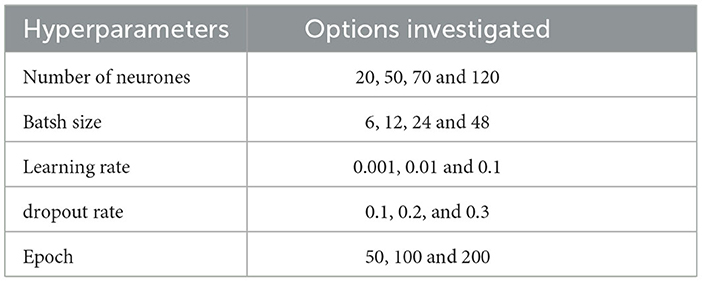
Table 3. Hyperparameters options investigated.

2.7. Model evaluation criteria

Three prediction performance evaluation indices were used, namely, mean absolute error (MAE), root mean squared error (RMSE) and the R². The MAE measures the average magnitude of errors in a set of predictions, regardless of their direction. It is the average, over the training or test sample, of the absolute differences between the prediction and the actual observation, with all individual differences having the same weight. It is less sensitive to outliers, making it more suitable for cases where extreme values might be present in the dataset. The RMSE is a quadratic scoring rule that also measures the average magnitude of the error. It is the square root of the average of the squared differences between the prediction and the actual observation. RMSE ensures that outliers and large errors have a substantial impact on the evaluation, providing a more robust assessment of the model's performance. R² is an indicator used in data analysis to judge the quality of a model and to measure the degree of accuracy in reproducing observed values, R² values are between (0, 1) where an R² score close to 1 represents optimal model prediction. The selection of performance indices in this study is based on their widespread use and established importance in hydrogeological modeling, including groundwater level prediction (Rajaee et al., 2019).

$\begin{array}{ll}MAE=\frac{1}{n}{\sum }_{j=1}^n|y_j-\widehat{y_j}|& (11)\end{array}$

$\begin{array}{ll}RMSE=\sqrt{\frac{1}{n}{\displaystyle {\sum }_{j=1}^n(y_j-{\widehat{y_j)}}^2}}& (12)\end{array}$

$\begin{array}{ll}{R}^2=\frac{{\displaystyle {\sum }_{j=1}^n{(y_j-\overline{y_j})}^2}-{\displaystyle {\sum }_{j=1}^n(y_j-{\widehat{y_j)}}^2}}{{\displaystyle {\sum }_{j=1}^n{(y_j-\overline{y_j})}^2}}& (13)\end{array}$

where y_j is the measured value at time j, $\overline{y_j}$is the average of y_j (j= 1,..., N) and i $\widehat{y_j}$ is the predicted value at time j.

3. Results

3.1. Input variable selection

The groundwater level shows very distinct correlation values with the input variables and within the five wells (Figure 4). In well P1, the groundwater level shows a weak correlation with NDVI and evapotranspiration; on the other hand it shows a slight positive correlation with precipitation (0.3) and negative correlation with land surface temperature (−0.3). The groundwater level in well P2 has low correlations with the four input variables, the highest correlation is 0.21 obtained with evapotranspiration. Well P3 shows relatively high positive correlation values of groundwater level with NDVI (0.43) and evapotranspiration (0.39), while precipitation and land surface temperature show no significant correlations. The level of groundwater in well P4 shows slight correlation values with NDVI (0.28) and evapotranspiration (0.3). In well P5, the level of groundwater has weak correlations with all four input variables, and the correlation value that is slightly high (0.28) is observed with evapotranspiration (Figure 4). Moreover, it can be observed that within the five wells. the input variables exhibit strong correlations (both positive and negative) among themselves.

FIGURE 4

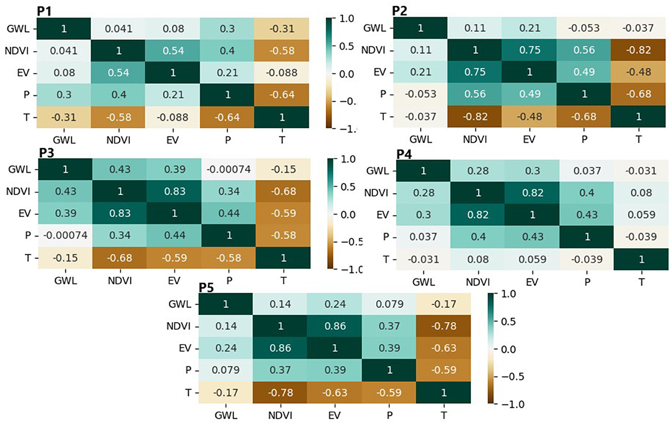
Figure 4. Correlation heath-map of groundwater level of the five wells with NDVI, MODIS Land surface temperature (T), MODIS evapotranspiration (EV) and IMERG-GPM precipitation (P).

The benefit of using XGBoost is that once the boosted trees are constructed, it is quite simple to retrieve the importance scores for each variable. The XGBoost result shows that land surface temperature is the most important input variable for groundwater level in the wells P1 and P5. Furthermore, precipitation, NDVI, and evapotranspiration are the important input variables, respectively, for P2, P3, and P4 (Figure 5). Thus, based on these results, the most important input variable for each well is used as a predictor variable in the LSTM-XGB-GS model.

FIGURE 5

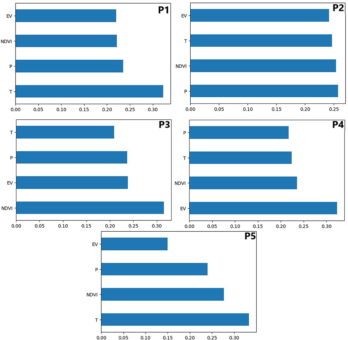
Figure 5. Input features importance for each well using XGBoost.

3.2. Hyperparameter tuning results

The outcomes of hyperparameter tuning reveal a notable distinction between the LSTM-XGB-GS model and the LSTM-GS model. Conversely, for each individual model, the differences are relatively minor across the wells (Table 4). In the case of the LSTM-XGB-GS model, the optimal number of neurons is 70, except for well P2 where it is 50. The preferred batch size is 48 for wells P1, P2, and P3, 24 for well P4, and 12 for well P5. Across most wells, the favored learning rate is 0.001, with the exception of well P5 where it is 0.01. The highest dropout rate (0.3) is utilized for wells P1, P4, and P5, while for wells P2 and P3, the optimal dropout rate is 0.2. The optimal number of epochs for all wells stands at 200.

TABLE 4

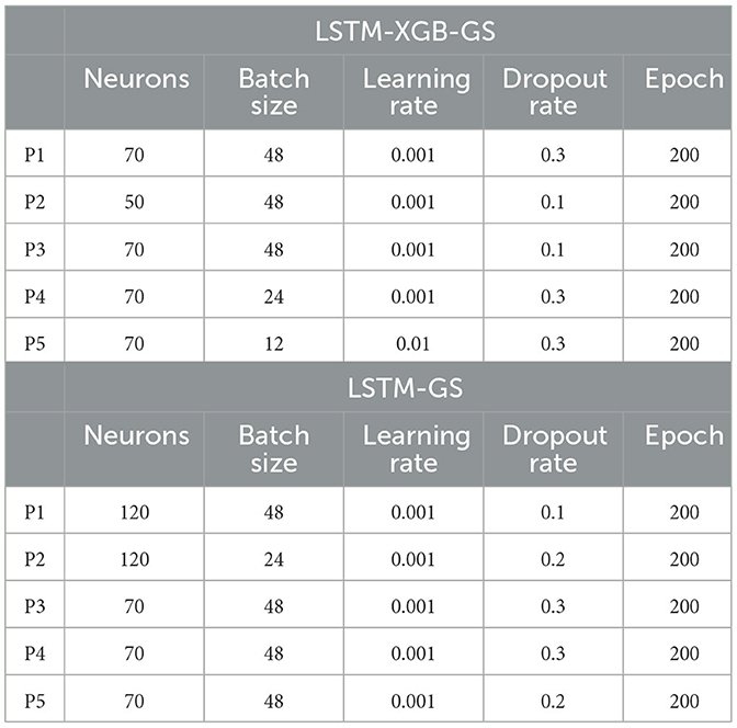
Table 4. Hyperparameters tuning for LSTM models.

For the LSTM-GS model, the most effective number of neurons is 120 for wells P1 and P2, and 70 for wells P3, P4, and P5. The optimal batch size across all wells, except for well P2, is 48. Well P2 features a batch size of 24. Learning rates of 0.001 are consistent across all wells. The highest dropout rate (0.3) is employed for wells P3 and P4, while for wells P2 and P5, the ideal dropout rate is 0.2, and for P1 it's 0.1. The optimum number of epochs remains consistent at 200 for all wells.

These results highlight the sensitivity of the LSTM model to the quantity and selection of input data, a factor that can have an impact on the results of individual models and wells.

3.3. Assessment of model performance using evaluation criteria

The performance of the models, in terms of three statistical indices during both the training and test periods, is presented in Table 4. The optimized model with the best input feature (LSTM-XGB-GS) demonstrated significantly superior performance compared to both the optimized model with all input features (LSTM-GS) and the standalone model (LSTM) across all five wells.

The R² values of the LSTM-XGB-GS model during the training period ranged from 0.95 to 0.99, while the corresponding values for LSTM-GS and LSTM were found to be in the range of 0.89 to 0.99 and 0.67 to 0.84, respectively. Upon analyzing the computed RMSE and MAE values, it was observed that the LSTM-XGB-GS model achieved the minimum values for all five studied wells. The RMSE ranged from 0.03 to 0.68 meters, while the MAE ranged from 0.03 to 0.51 meters. Specifically, the wells in the irrigated areas P1 and P2, as well as those in the floodplain P3 and P4, exhibited acceptable values of RMSE (0.33 m, 0.57 m, 0.68 m, and 0.25 m, respectively) and MAE (0.22 m, 0.45 m, 0.51 m, and 0.20 m, respectively). Notably, the P5 well located on the phosphate plateau demonstrated the lowest values of RMSE (0.03 m) and MAE (0.02 m). Furthermore, it is worth mentioning that the LSTM model showed the lowest modeling performance in terms of RMSE and MAE during the training period.

During the test period, the LSTM-XGB-GS model demonstrated good to excellent performance, achieving an R² between 0.72 and 0.99. On the other hand, the LSTM-GS model exhibited varying performance, ranging from poor to excellent depending on the well location, with an R² between 0.27 and 0.97. Meanwhile, the LSTM standalone model showed the poorest performance across all five wells, attaining an R² between 0.09 and 0.96.

As for the RMSE and MAE indices, the LSTM-XGB-GS model consistently displayed the lowest values among the three models for all five wells. In particular, when utilizing MODIS LST as the input variable for well P1, the LSTM-XGB-GS model yielded RMSE and MAE values of 0.20 m and 0.15 m, respectively (Table 5). For well P2, employing IMERG-GPM precipitation as the input, the LSTM-XGB-GS model resulted in RMSE and MAE values of 0.66 m and 0.58 m, respectively. For well P3, using MODIS NDVI as the input, the model provided acceptable RMSE and MAE values of 0.42 m and 0.39 m, respectively. Similarly, well P4, with MODIS evapotranspiration as the input, demonstrated acceptable RMSE and MAE values of 0.35 m and 0.29 m, respectively. Notably, the phosphate plateau well P5, utilizing MODIS LST, exhibited the best prediction performance during the test period, with both RMSE and MAE values at 0.02 m.

TABLE 5

Table 5. Models evaluation criteria for groundwater level prediction during training and testing periods.

3.4. Assessment of model performance using scatter plots and time series plot

The scatter plots of groundwater levels observed and predicted using the three models during the training and test periods are shown in Figure 6. In general, the results show that the groundwater level predicted by the three models closely reflect, or even align with, the trend in the observed data (the black line) during the training period. This alignment is also supported by the R² values, which exceed 0.7 for all models over the five wells (Table 5). It should be noted, however, that the scatterplot associated with the LSTM-XGB-GS model adheres more closely to the trend in the observed data than the scatterplots for the LSTM-GS model and the stand-alone LSTM model. The latter two show slightly more dispersed scatterplots, with some values far from the trend of the observed data.

FIGURE 6

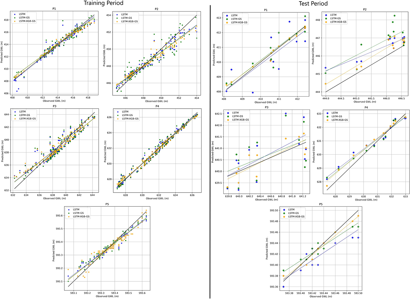
Figure 6. Scatterplots of groundwater levels observed and predicted by the three models over the training and test periods.

The results from the test period give a clearer overview of the prediction performance of the models compared with the results from the training period. Most notably, the scatter plot for the LSTM-XGB-GS model shows better alignment with the trend in the observed data, with points showing reduced dispersion and closer proximity to the trend line. Conversely, the scatterplots of the LSTM-GS and standalone LSTM models are less closely aligned with the trend of the observed data, with points showing increased scatter. These observations are also supported by the R² values, where the LSTM-XGB-GS model has the highest values for all five wells (Table 5).

Time series plots of monthly variations in groundwater levels observed and predicted over the test period by the three models is shown in Figure 7. The plots show that all three models effectively capture seasonal fluctuations and variations in groundwater levels in each well. However, the LSTM-XGB-GS model shows superior performance in reproducing the groundwater levels observed. It shows remarkable alignment with minimal overestimation or underestimation. In particular, for wells P1 and P4, the LSTM-XGB-GS model almost perfectly reproduces the observed data. On the other hand, the LSTM-GS and standalone LSTM models, although capable of capturing seasonal variations in groundwater levels, show significant overestimates and underestimates. This discrepancy is most pronounced, although slightly attenuated, in well P4, where the values of the latter two models are very close to the observed data.

FIGURE 7

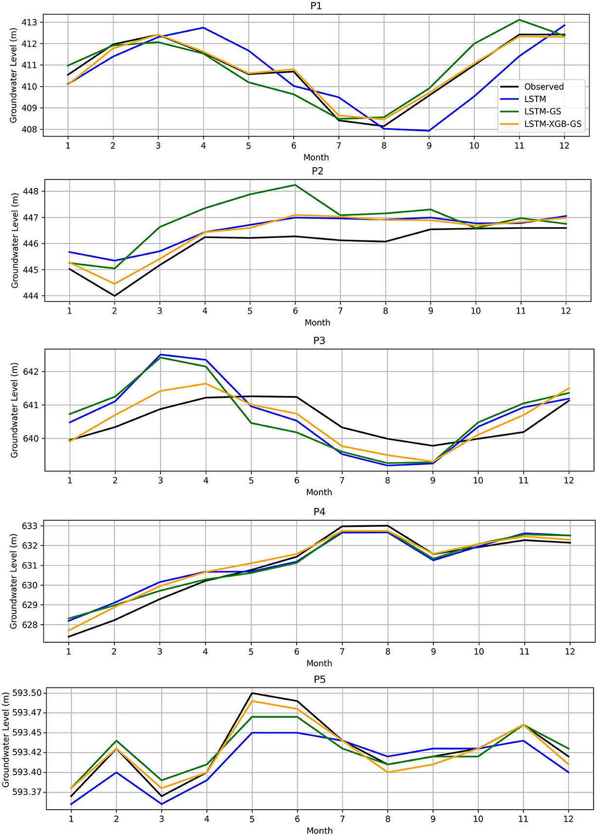
Figure 7. Monthly variations of groundwater level observed and predicted over the test period.

3.5. Assessment of models performance using violin plot and Taylor diagram

Finally, the ability of the three models to reproduce the probability distribution of observed groundwater level data during the training and test periods for all five wells was visually evaluated by preparing violin plots. The violin plots displaying the observed and predicted groundwater level data by the models during the training period are presented in Figure 8. The violin plots demonstrate that all three models have a similar overall shape to the observed groundwater level data, with their median values closely aligned, suggesting similarity in the distribution of predicted and observed groundwater level data. However, it was also observed that the violin plots of the LSTM-XGB-GS model appear slightly narrower compared to the other models and the observed data for wells P1, P2, P3, and P5. This indicates a slightly lower variance in the predictions. Additionally, the LSTM-XGB-GS model shows a slight tendency to underestimate maximum values and overestimate minimum values for these wells. On the other hand, the LSTM-GS model exhibits a high degree of similarity with the observed data for wells P1, P2, and P4, without underestimating or overestimating extreme values. In contrast, the LSTM model shows some divergence from the observed data, with underestimation and overestimation of maximum and minimum values, except for well P4, where the LSTM model exhibits a distribution similar to the observed values.

FIGURE 8

Figure 8. Violin plots showing the relative performance of the three models in replicating distribution of observed groundwater level data during the training and test periods.

The violin plots of the test period show that the LSTM-XGB-GS model exhibits the highest similarity to the observed data compared to the other two models (Figure 8). For wells P1, P4, and P5, the LSTM-XGB-GS model displays a similar shape and range to the observed data, with a median value at the same level and less underestimation and overestimation of the maximum and minimum values compared to the other models. For well P2, all three models overestimate the median and extreme values compared to the observed data, but the LSTM-XGB-GS model shows the lowest divergence and a shape similar to the observed data. For well P3, all three models display a wider shape than the observed data; however, the LSTM-XGB-GS model exhibits the least divergence by showing a median value at the same level as the observed data, with the lowest overestimation and underestimation of extreme values.

The performances of the different models were also assessed using the Taylor diagram. The Taylor diagram graphically compares two statistics, namely the standard deviation and correlation, to provide a reliable and more direct evaluation of the relative performance of the different models. The results for the five wells are presented in Figure 9. In the Taylor diagram, the dashed black circle represents the observed groundwater level, and the black star denotes the reference point for the observed data. A model is considered proficient if it is close to the reference point. During the training period (Figure 9), the LSTM-XGB-GS model exhibited the best performance across all five wells. On the other hand, the standalone LSTM model showed the weakest performance in predicting the observed data. However, for well P5, the performances of the LSTM-XGB-GS and LSTM-GS models were roughly equal. For the results of the test period (Figure 9), the LSTM-XGB-GS model also displayed the best performance in predicting the observed data during the test period. Conversely, the standalone LSTM model demonstrated better performance than the LSTM-GS model for wells P2 and P3. However, for the P5 well, the performance of the LSTM-XGB-GS and LSTM-GS models was fairly equal compared to the standalone LSTM model, whose performance was much lower.

FIGURE 9

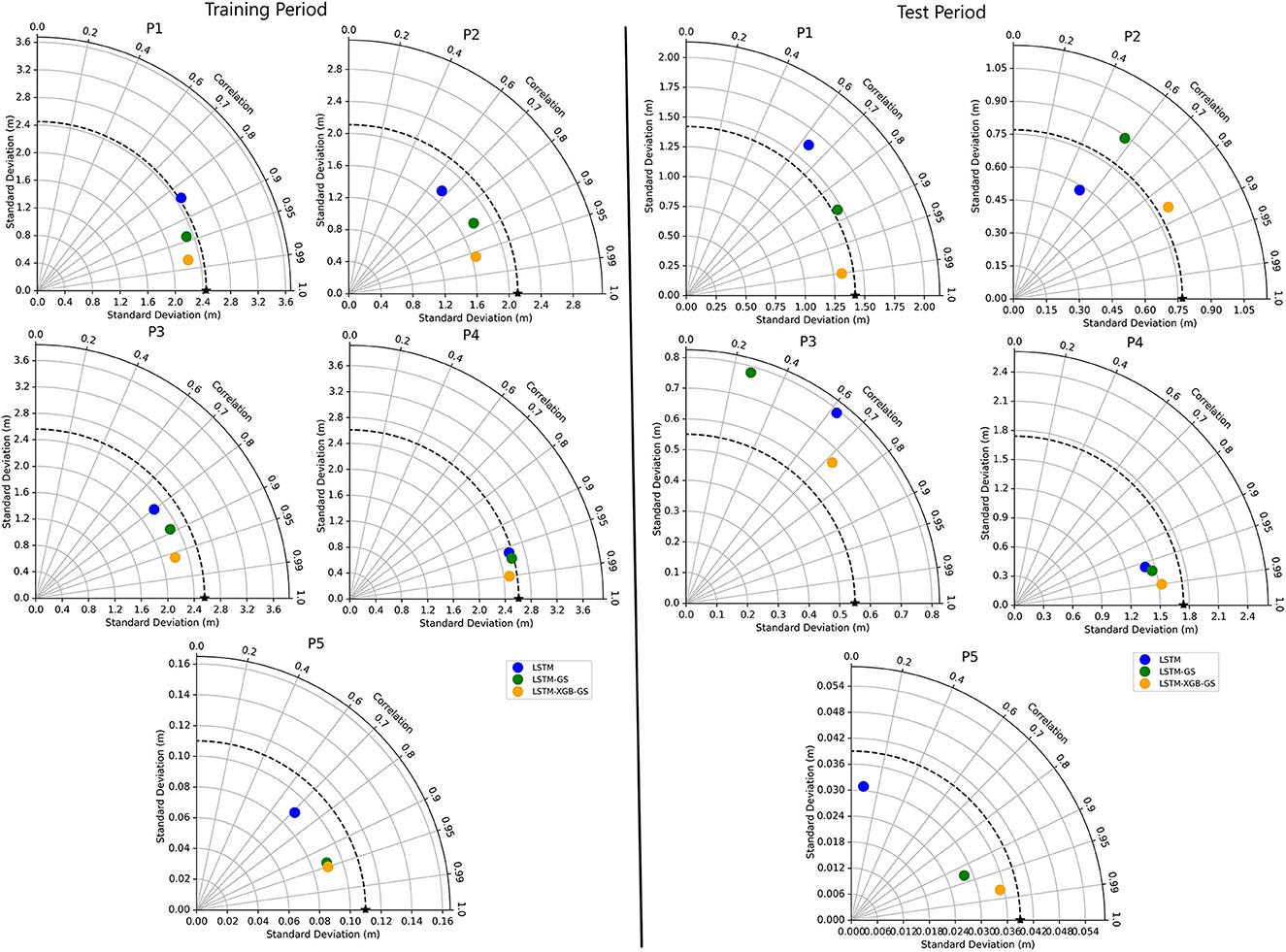
Figure 9. Taylor diagram representing the statistical performance of the three models in predicting observed groundwater level data during the training and test periods.

4. Discussion

4.1. Importance of the input feature selection and model optimization on groundwater prediction

The good performance achieved by the LSTM-XGB-GS model in this study clearly emphasizes the importance and impact of identifying the best input feature and fine-tuning the hyperparameters for groundwater level prediction. The hydrodynamic characteristics of aquifers and the groundwater levels fluctuation in monitoring wells exhibit significant variations influenced by several factors (Rinderer et al., 2016; Iqbal et al., 2020; Band et al., 2021), primarily encompassing hydro-geodynamic and climatic conditions, as well as land use and land cover. To achieve enhanced model performance, it becomes imperative to pinpoint the variable that reflects the dominant factor that explains most the variation of the groundwater level in each well. Moreover, the optimization of the LSTM model's hyperparameters using the GridSearchCV method enables a more effective capture of patterns and relationships between groundwater level and the selected remote sensing variable.

However, it is worth noting that the number of observed values in the five wells averages 134, which represents a relatively small dataset for ensuring the LSTM model's optimal performance. LSTM model initially designed for learning on large datasets, commonly known as “big data,” shows remarkable performance. However, the model's formidable learning capacity can present difficulties when applied to a limited dataset of groundwater level observations. In such cases, the LSTM model becomes susceptible to over-fitting, which can compromise its predictive accuracy (Baek and Kim, 2018). This overfitting issue is evident in the case of the LSTM-GS model. By employing all available remote sensing variables without specifically selecting the most informative ones for each well, the LSTM-GS model becomes overly specialized in capturing the training data, leading to decreased performance when confronted with new, unseen data during the testing phase (Table 5). Furthermore, the poor performance of the LSTM standalone model was expected, since it uses all available input variables without the hyperparameters optimization. As a result, this model is prone to overfitting and its ability to accurately capture fluctuations in groundwater levels is limited. This has been observed in several other studies, where standalone ANN models exhibited the weakest performance in predicting groundwater variables (Rahman et al., 2020; Cui et al., 2022; Zhang et al., 2023).

4.2. Model performance assessment in irrigated and floodplain areas

Despite the high fluctuation of groundwater levels in well P1 (Standard deviation > 2 m) (Table 2), the integration of the best input feature (MODIS LST) using XGBoost and the hyperparameter optimization of the LSTM-XGB-GS model led to a remarkably accurate prediction of its groundwater levels during the test period (Figure 7). This good prediction performance can be attributed to the relationship between irrigation and land surface temperature, as evidenced by several studies (Bright et al., 2017; Liu et al., 2019; Yang et al., 2020; Zhang Z. et al., 2022). These studies, demonstrated that in arid regions, irrigation has been shown to substantially alter the land surface temperature, resulting in lower daytime land surface temperature in irrigated areas compared to adjacent non-irrigated regions (Yang et al., 2020). Given that irrigation in the Beni Moussa aquifer heavily relies on pumping water from the aquifer (Lionboui et al., 2021), a direct relationship may exist between the dynamics of groundwater levels and the variations in land surface temperature. Consequently, this interplay between land surface temperature and groundwater levels could explain LSTM-XGB-GS model's good performance in simulating groundwater levels for well P1.

The LSTM-XGB-GS prediction results for wells P2 and P3 are generally acceptable and reliable. However, a noticeable decrease in model prediction performance is observed when compared to their training period or to the other wells (Table 5). This decrease in performance can be attributed to several factors. To begin with, the correlation coefficient for groundwater level in well P2 does not exhibit a distinct correlation with any of the four input variables (Figure 4). XGBoost indicates that IMERG-GPM precipitation is ranked first, but it is not isolated from the other variables since they all hold roughly the same level of importance (Figure 5). This observation might be explained by the significant unsaturated zone at well P2, where the depth to the water table is 36.78 m (Table 2). At certain depths, surface climatic conditions such as land surface temperature and evapotranspiration may have only a minor influence on short-term groundwater fluctuations. Conversely, changes in the precipitation regime can have a long-term impact on groundwater levels. Nevertheless, the effect of precipitation on groundwater is not always immediate; it can vary from month to month and is heavily dependent on the aquifer's hydrological conditions (Jan et al., 2013; Grinevskii, 2014; Cai and Ofterdinger, 2016; Qi et al., 2018; Mogaji and Lim, 2020). Moreover, the IMERG-GPM product's low spatial resolution (10 km) might hinder its ability to accurately capture the fine-scale spatial variability in precipitation, which is crucial in this semi-arid irrigated plain (Ouatiki et al., 2019). Additionally, numerous evaluations of the IMERG-GPM product have revealed certain biases and estimation errors, leading to significant over- and underestimations of the duration and intensity of precipitation (Ramsauer et al., 2018; Ouatiki et al., 2019; Kazamias et al., 2022; Pradhan et al., 2022).

In addition, NDVI exhibits a strong positive correlation with well P3 in the floodplain (Figure 4), supporting the findings of XGBoost, where NDVI is identified as the most important input feature. This good correlation/importance can be attributed to the temporal variation of NDVI in floodplain areas, where it has been shown to effectively capture seasonal and inter-annual variability in vegetation dynamics and the hydro-sedimentological regime along and across the floodplain (Shrestha et al., 2013; Powell et al., 2014; Marchetti et al., 2016). Moreover, NDVI values provide insights into the relationship between groundwater and plant growth. In cases where a high NDVI area is experiencing drought, it indicates that vegetation is consuming more groundwater, which potentially impact groundwater levels variation (Hassan et al., 2019; Hadri et al., 2021; Lebrini et al., 2021; Moumane et al., 2021; Sajjad et al., 2022; Zhang Z. et al., 2022). However, given the positioning of well P3 in the floodplain, it is plausible that the influence of the nearby wadi contributes significantly to the observed decline in model performance between the training and test periods. The dynamic interactions that occur between the wadi and the aquifer have the potential to elucidate a substantial part of the fluctuations observed in the water table, as highlighted by previous studies (May et al., 2011; Wang et al., 2014; Kazamias et al., 2022). To establish this hypothesis with greater certainty, a more conclusive assessment of the modeling performance would require the integration of flow data from the wadi. Unfortunately, such data were not available in the present case.

The strong relationship between groundwater levels in well P4 and MODIS evapotranspiration (Figures 4, 5) clearly enabled accurate prediction of groundwater level fluctuations in this well. This can be explained by the fact that the floodplains in this region serve as designated irrigation areas, used to extract water from surface and groundwater reservoirs. This is particularly important during prolonged periods of limited rainfall, when the extracted water supports plant growth, resulting in increased evapotranspiration (Zhang et al., 2018; Hssaisoune et al., 2020; Ahmed et al., 2021; Malakar et al., 2021). In this context, the measurement of evapotranspiration is of key importance and is considered an essential climatic parameter for vigilant monitoring and effective management of irrigation operations and floodplain ecosystems. Many research studies have seamlessly integrated evapotranspiration data acquired from remote sensing resources, including MODIS data, to assess irrigation needs and decipher hydrological models (Droogers et al., 2010; Van Houdt et al., 2020; Vogels et al., 2020).

It's important to acknowledge that groundwater resources in irrigated and floodplain areas bear a substantial impact from intensive pumping activities (Zhang et al., 2018; Malakar et al., 2021). This phenomenon accounts for the substantial fluctuations in groundwater levels within irrigated (wells P1 and P2) and floodplain (wells P3 and P4) regions, as evidenced by their high standard deviations (> 2m) (Table 2). The influence of farming practices, particularly irrigation and pumping, is even more pronounced in semi-arid and arid climates, where high pressure and reliance on groundwater are prevalent during water scarcity periods (Wang et al., 2014; Kirby et al., 2015; Mao et al., 2017; Pulido-Bosch et al., 2018; Salem et al., 2018; Tweed et al., 2018; Cavelan et al., 2022). In Morocco, the combination of meteorological drought driven by reduced rainfall and elevated temperatures has escalated irrigation water demand. Consequently, irrigation sources often shift from surface water to groundwater during these periods. Such challenges have been closely monitored and evaluated across the OER Basin and its irrigated areas, where human activities have exerted significant pressure on water resources, leading to notable declines in groundwater levels averaging from 71.9 to 148.8 cm/year (Ahmed et al., 2021) and ~30 m over the past three decades (Hssaisoune et al., 2020). As a consequence, the model prediction performances highlight the importance of precise knowledge regarding groundwater pumping rates and volumes. Such information proves critical for enhancing future groundwater modeling and forecasting in arid and semi-arid climates characterized by intense irrigation and pumping activities. These insights enable effective training of models to adeptly capture the abrupt shifts in hydraulic head that result from these activities. However, the challenge often lies in obtaining accurate data concerning the quantity of water pumped from individual wells (Trichakis et al., 2011).

4.3. Model performance assessment of a stationary groundwater level

Well P5, located in the phosphate plateau area, achieves the best modeling results during the training and testing periods in both LSTM-XGB-GS and LSTM-GS models (Table 5), and the simulated groundwater level maintains the same trend, distribution and quasi-stationary aspect of the observed groundwater level variation. This result was anticipated given that well P5 have the lowest groundwater level fluctuation (standard deviation of 0.11 m) and the deepest water table depth (mean depth of 72 m) (Table 2). These aspects suggest that groundwater levels in well P5 remain relatively unaffected by climatic conditions or surface activities such as irrigation or pumping, as demonstrated by the low correlation values of the groundwater level with the four input variables (Figure 4). In general, groundwater level prediction studies that have shown excellent performance (RMSEs and MAEs < 0.1 m), have often been applied to groundwater levels that did not show large groundwater fluctuations, or they showed a long-term trend, over the whole time series (Bowes et al., 2019; Band et al., 2021; Ghazi et al., 2021; Wunsch et al., 2021). This near-stationary or regular dynamics allow ANN models, and in particular recurrent neural networks such as the LSTM, to adequately predict the time series, as the output variable becomes increasingly easy to predict as the time series advances. in such conditions, it would be possible to predict the groundwater level of the well P5 by adopting only a univariate prediction approach, which relies solely on the groundwater level observed data as input to the LSTM optimized model (Raghavendra and Deka, 2016; Mohanasundaram et al., 2019; Roy et al., 2021; Sarma and Singh, 2022).

5. Conclusion

The primary goal of this study is to assess the contribution of remote sensing data and the input feature selection approach within neural network models to predict groundwater levels in the OER basin in Morocco. This region faces great challenges such as drought and excessive groundwater water resource usage due to intense irrigation. These challenges highlight the urgent need for dependable and precise groundwater level prediction techniques. To achieve this, three LSTM models for groundwater level prediction were developed, rigorously analyzed and compared. The first LSTM model, named LSTM-XGB-GS, was optimized using the GridsearchCV method, and uses a single variable identified by the XGBoost method. This selected variable is considered the most effective in explaining variations in groundwater level among four remotely sensed variables: GPM precipitation, MODIS NDVI, MODIS evapotranspiration, and MODIS LST. Another optimized LSTM model was also constructed, but uses the four variables as input (LSTM-GS). Additionally, a standalone LSTM model was established and also incorporating the four variables as inputs. The performance prediction of these models was evaluated in five wells strategically located across diverse areas within the Tadla plain in Morocco. Specifically, two wells (P1 and P2) are located in irrigated zones, another two wells (P3 and P4) are positioned in alluvial floodplains, and one well (P5) is situated on the plateau region recognized as the Phosphate Plateau.

The results of the study demonstrate the consistent outperformance of the LSTM-XGB-GS model compared with the LSTM-GS model and the standalone LSTM model. The LSTM-XGB-GS model demonstrates remarkable accuracy during both training and test periods, as evidenced by high R² values, notably ranging from 0.95 to 0.99 during training periods and 0.72 to 0.99 during testing periods. Furthermore, the LSTM-XGB-GS model achieves the lowest RMSE and MAE values across all wells, illustrating its superior predictive capabilities. More specifically, well P1 demonstrates accurate predictions using the LSTM-XGB-GS model with MODIS LST as the optimal input, attributed to the connection between irrigation and land surface temperature. However, well P2 experiences reduced prediction performance of the LSTM-XGB-GS model due to its water table depth and limitations arising from the low spatial resolution of IMERG-GPM data. Despite a strong NDVI correlation with groundwater levels in the floodplain well P3, the low prediction performance of LSTM-XGB-GS model could potentially be influenced by interactions with the wadi flow. In the floodplain well P4, the significant relationship between groundwater levels and MODIS evapotranspiration notably enhances the LSTM-XGB-GS predictions performance. Lastly, the low variation groundwater levels of well P5 contribute to robust model predictions, enabling accurate prediction due to its distinctive characteristics.

Finally, this study demonstrates the support that remote sensing data can provide for groundwater prediction using the ANNs model in conditions where in situ data are lacking. It's also highlights the distinctive characteristics and behavior of groundwater levels in each well, which can be attributed to well construction, hydrodynamic conditions, aquifer characteristics, and the type of land cover and land use. Consequently, there is a pronounced need to develop a generalized neural network model structure, architecture, and generalized input variables, enabling faster and more efficient predictions of groundwater levels for multiple wells simultaneously at the basin scale.

Data availability statement

The raw data supporting the conclusions of this article will be made available by the authors on request.

Author contributions

TB, ML, and IK contributed to the design and development of the study. HO and AB organized the database. ML performed the statistical analysis. TB wrote the first version of the manuscript. TB, ML, AB, and HO wrote parts of the manuscript. All authors contributed to the article and approved the submitted version.

Acknowledgments

This work was carried out at the geoscience, water and environment laboratory of the Faculty of Sciences of Rabat Mohammed V University in Rabat and at the Institute for Development Research (IRD). The authors also acknowledge the availability of in situ observations from Oum Er-Rbia Basin agency.

Conflict of interest

The authors declare that the research was conducted in the absence of any commercial or financial relationships that could be construed as a potential conflict of interest.

Publisher's note

All claims expressed in this article are solely those of the authors and do not necessarily represent those of their affiliated organizations, or those of the publisher, the editors and the reviewers. Any product that may be evaluated in this article, or claim that may be made by its manufacturer, is not guaranteed or endorsed by the publisher.

References

Adams, K. H., Reager, J. T., Rosen, P., Wiese, D. N., Farr, T. G., Rao, S., et al. (2022). Remote sensing of groundwater: current capabilities and future directions. Water Res. Res. 58, e2022WR. doi: 10.1029/2022WR032219

CrossRef Full Text | Google Scholar

Ahmed, M., Aqnouy, M., and El Messari, J. S. (2021). Sustainability of Morocco's groundwater resources in response to natural and anthropogenic forces. J. Hydrol. 603, 126866. doi: 10.1016/j.jhydrol.2021.126866

CrossRef Full Text | Google Scholar

Anh, D. T., Pandey, M., Mishra, V. N., Singh, K. K., Ahmadi, K., Janizadeh, S., et al. (2023). Assessment of groundwater potential modeling using support vector machine optimization based on Bayesian multi-objective hyperparameter algorithm. Appl. Soft Comput. 132, 109848. doi: 10.1016/j.asoc.2022.109848

CrossRef Full Text | Google Scholar

Azzali, S., and Menenti, M. (2000). Mapping vegetation-soil-climate complexes in southern Africa using temporal fourier analysis of NOAA-AVHRR NDVI data. Int. J. Remote Sens. 21, 973–996. doi: 10.1080/014311600210380

CrossRef Full Text | Google Scholar

Baek, Y., and Kim, H. Y. (2018). ModAugNet: A new forecasting framework for stock market index value with an overfitting prevention LSTM module and a prediction LSTM module. Expert Syst. Appl. 113, 457–480. doi: 10.1016/j.eswa.2018.07.019

CrossRef Full Text | Google Scholar

Band, S. S., Heggy, E., Bateni, S. M., Karami, H., Rabiee, M., Samadianfard, S., et al. (2021). Groundwater level prediction in arid areas using wavelet analysis and Gaussian process regression. Eng. Appl. Comput. Fluid Mech. 15, 1147–1158. doi: 10.1080/19942060.2021.1944913

CrossRef Full Text | Google Scholar

Becker, M. W. (2006). Potential for satellite remote sensing of ground water. Groundwater 44, 306–318. doi: 10.1111/j.1745-6584.2005.00123.x

PubMed Abstract | CrossRef Full Text | Google Scholar

Bhanja, S. N., Malakar, P., Mukherjee, A., Rodell, M., Mitra, P., Sarkar, S., et al. (2019). Using satellite-based vegetation cover as indicator of groundwater storage in natural vegetation areas. Geophys. Res. Lett. 46, 8082–8092. doi: 10.1029/2019GL083015

CrossRef Full Text | Google Scholar

Bikše, J., Retike, I., Haaf, E., and Kalvāns, A. (2023). Assessing automated gap imputation of regional scale groundwater level data sets with typical gap patterns. J. Hydrol. 620, 129424. doi: 10.1016/j.jhydrol.2023.129424

CrossRef Full Text | Google Scholar

Bowes, B. D., Sadler, J. M., Morsy, M. M., Behl, M., and Goodall, J. L. (2019). Modelling groundwater table in a flood prone coastal city with long short-term memory and recurrent neural networks. Water 11, 1098. doi: 10.3390/w11051098

CrossRef Full Text | Google Scholar

Breiman, L., Friedman, J. H., Olshen, R. A., and Stone, C. J. (2017). Classification and Regression Trees. London: Routledge.

Google Scholar

Bright, R. M., Davin, E., O'Halloran, T., Pongratz, J., Zhao, K., Cescatti, A., et al. (2017). Local temperature response to land cover and management change driven by non-radiative processes. Nat. Clim. Change 7, 296–302. doi: 10.1038/nclimate3250

CrossRef Full Text | Google Scholar

Cabaneros, S. M., Calautit, J. K., and Hughes, B. R. (2019). A review of artificial neural network models for ambient air pollution prediction. Environ. Modell. Software 119, 285–304. doi: 10.1016/j.envsoft.2019.06.014

CrossRef Full Text | Google Scholar

Cai, Z., and Ofterdinger, U. (2016). Analysis of groundwater-level response to rainfall and estimation of annual recharge in fractured hard rock aquifers, NW Ireland. J. Hydrol. 535, 71–84. doi: 10.1016/j.jhydrol.2016.01.066

CrossRef Full Text | Google Scholar

Cavelan, A., Golfier, F., Colombano, S., Davarzani, H., Deparis, J., Faure, P., et al. (2022). A critical review of the influence of groundwater level fluctuations and land surface temperatureon LNAPL contaminations in the context of climate change. Sci. Total Environ. 806, 150412. doi: 10.1016/j.scitotenv.2021.150412

PubMed Abstract | CrossRef Full Text | Google Scholar

Chang, Z., Lu, W., and Wang, Z. (2022). Study on source identification and source-sink relationship of LNAPLs pollution in groundwater by the adaptive cyclic improved iterative process and Monte Carlo stochastic prediction. J. Hydrol. 612, 128109. doi: 10.1016/j.jhydrol.2022.128109

CrossRef Full Text | Google Scholar

Chawla, I., Karthikeyan, L., and Mishra, A. K. (2020). A review of remote sensing applications for water security: quantity, quality, and extremes. J. Hydrol. 585, 124826. doi: 10.1016/j.jhydrol.2020.124826

CrossRef Full Text | Google Scholar

Chen, X., Zhao, X., Tahmasebi, P., Luo, C., and Cai, J. (2023). NMR-data-driven prediction of matrix permeability in sandstone aquifers. J. Hydrol. 618, 129147. doi: 10.1016/j.jhydrol.2023.129147

CrossRef Full Text | Google Scholar

Chen, Y., Song, L., Liu, Y., Yang, L., and Li, D. (2020). A review of the artificial neural network models for water quality prediction. Appl. Sci.nces 10, 5776. doi: 10.3390/app10175776

CrossRef Full Text | Google Scholar

Coulibaly, P., Anctil, F., Aravena, R., and Bobée, B. (2001). Artificial neural network modeling of water table depth fluctuations. Water Res. Res. 37, 885–896. doi: 10.1029/2000WR900368

PubMed Abstract | CrossRef Full Text | Google Scholar

Cui, F., Al-Sudani, Z. A., Hassan, G. S., Afan, H. A., Ahammed, S. J., Yaseen, Z. M., et al. (2022). Boosted artificial intelligence model using improved alpha-guided grey wolf optimizer for groundwater level prediction: comparative study and insight for federated learning technology. J. Hydrol. 606, 127384. doi: 10.1016/j.jhydrol.2021.127384

CrossRef Full Text | Google Scholar

Daliakopoulos, I. N., Coulibaly, P., and Tsanis, I. K. (2005). Groundwater level modelling using artificial neural networks. J. Hydrol. 309, 229–240. doi: 10.1016/j.jhydrol.2004.12.001

CrossRef Full Text | Google Scholar

Derbela, M., and Nouiri, I. (2020). Intelligent approach to predict future groundwater level based on artificial neural networks (ANN). Euro-Mediter. J. Environ. Int. 5, 1–11. doi: 10.1007/s41207-020-00185-9

CrossRef Full Text | Google Scholar

Dormann, C. F., Elith, J., Bacher, S., Buchmann, C., Carl, G., Carr,é, G., et al. (2013). Collinearity: a review of methods to deal with it and a prediction study evaluating their performance. Ecography 36, 27–46. doi: 10.1111/j.1600-0587.2012.07348.x

CrossRef Full Text | Google Scholar

Droogers, P., Immerzeel, W. W., and Lorite, I. J. (2010). Estimating actual irrigation application by remotely sensed evapotranspiration observations. Agric. Water Manage. 97, 1351–1359. doi: 10.1016/j.agwat.2010.03.017

PubMed Abstract | CrossRef Full Text | Google Scholar

Dumont, A. (2021). Acting Together for the Sustainable Use of Water in Agriculture: Proposals to Prevent the Deterioration and Overexploitation of Groundwater. Paris: Éditions AFD.

Google Scholar

El Bilali, A., Taleb, A., and Brouziyne, Y. (2021). Comparing four machine learning model performances in modelling the alluvial aquifer level in a semi-arid region. J. African Earth Sci. 181, 104244. doi: 10.1016/j.jafrearsci.2021.104244

CrossRef Full Text | Google Scholar

Elshall, A. S., Castilla-Rho, J., El-Kadi, A. I., Holley, C., Mutongwizo, T., Sinclair, D., et al. (2022). Sustainability of Groundwater Imperiled: The Encyclopedia of Conservation. Amsterdam: Elsevier.

Google Scholar

Elzain, H. E., Chung, S. Y., Venkatramanan, S., Selvam, S., Ahemd, H. A., Seo, Y. K., et al. (2022). Novel machine learning algorithms to predict the groundwater vulnerability index to nitrate pollution at two levels of modeling. Chemosphere 137671. doi: 10.1016/j.chemosphere.2022.137671

PubMed Abstract | CrossRef Full Text | Google Scholar

Epting, J., Verbyla, D., and Sorbel, B. (2005). Evaluation of remotely sensed indices for assessing burn severity in interior Alaska using Landsat TM and ETM+. Remote Sens. Environ. 96, 328–339. doi: 10.1016/j.rse.2005.03.002

CrossRef Full Text | Google Scholar

Friedman, J. H. (2002). Stochastic gradient boosting. Comput. Stat. Data Anal. 38, 367–378. doi: 10.1016/S0167-9473(01)00065-2

CrossRef Full Text | Google Scholar

Fu, B., and Burgher, I. (2015). Riparian vegetation NDVI dynamics and its relationship with climate, surface water and groundwater. J. Arid Environ. 113, 59–68. doi: 10.1016/j.jaridenv.2014.09.010

CrossRef Full Text | Google Scholar

Gers, F. A., Schmidhuber, J., and Cummins, F. (2000). Learning to forget: continual prediction with LSTM. Neural Comput. 12, 2451–2471. doi: 10.1162/089976600300015015

PubMed Abstract | CrossRef Full Text | Google Scholar

Ghawi, R., and Pfeffer, J. (2019). Efficient hyperparameter tuning with grid search for text categorization using kNN approach with BM25 similarity. Open Comput. Sci. 9, 160–180. doi: 10.1515/comp-2019-0011

CrossRef Full Text | Google Scholar

Ghazi, B., Jeihouni, E., and Kalantari, Z. (2021). Simulating groundwater level fluctuations under climate change scenarios for Tasuj plain, Iran. Arabian J. Geosci. 14, 1–12. doi: 10.1007/s12517-021-06508-6

CrossRef Full Text | Google Scholar

Ghose, D., Das, U., and Roy, P. (2018). Modeling response of runoff and evapotranspiration for predicting water table depth in arid region using dynamic recurrent neural network. Groundwater Sust. Dev. 6, 263–269. doi: 10.1016/j.gsd.2018.01.007

CrossRef Full Text | Google Scholar

Graves, A. (2012). Supervised Sequence Labelling With Recurrent Neural Networks. Berlin: Springer, 5–13.

Google Scholar

Grinevskii, S. O. (2014). The effect of topography on the formation of groundwater recharge. Moscow Univ. Geol. Bullet. 69, 47–52. doi: 10.3103/S0145875214010025

CrossRef Full Text | Google Scholar

Hadri, A., Saidi, M. E. M., and Boudhar, A. (2021). Multiscale drought monitoring and comparison using remote sensing in a Mediterranean arid region: a case study from west-central Morocco. Arabian J. Geosci. 14, 1–18. doi: 10.1007/s12517-021-06493-w

CrossRef Full Text | Google Scholar

Hamed, Y., Hadji, R., Redhaounia, B., Zighmi, K., Bâali, F., El Gayar, A., et al. (2018). Climate impact on surface and groundwater in North Africa: a global synthesis of findings and recommendations. Euro-Mediter. J. Environ. Integ. 3, 1–15. doi: 10.1007/s41207-018-0067-8

CrossRef Full Text | Google Scholar

Hassan, M. A., Yang, M., Rasheed, A., Yang, G., Reynolds, M., Xia, X., et al. (2019). A rapid monitoring of NDVI across the wheat growth cycle for grain yield prediction using a multi-spectral UAV platform. Plant Sci. 282, 95–103. doi: 10.1016/j.plantsci.2018.10.022

PubMed Abstract | CrossRef Full Text | Google Scholar

Hastie, T., Tibshirani, R., Friedman, J. H., and Friedman, J. H. (2009). The Elements of Statistical Learning: Data Mining, Inference, and Prediction. New York, NY: Springer.

Google Scholar

Hochreiter, S. (1998). The vanishing gradient problem during learning recurrent neural nets and problem solutions. Int. J. Uncert. Fuzziness Syst. 6, 107–116. doi: 10.1142/S0218488598000094

CrossRef Full Text | Google Scholar

Hochreiter, S., and Schmidhuber, J. (1997). Long short-term memory. Neural Comput. 9, 1735–1780. doi: 10.1162/neco.1997.9.8.1735

PubMed Abstract | CrossRef Full Text | Google Scholar

Hssaisoune, M., Bouchaou, L., Sifeddine, A., Bouimetarhan, I., and Chehbouni, A. (2020). Moroccan groundwater resources and evolution with global climate changes. Geosciences 10, 81. doi: 10.3390/geosciences10020081

CrossRef Full Text | Google Scholar

Htitiou, A., Boudhar, A., Chehbouni, A., and Benabdelouahab, T. (2021). National-scale cropland mapping based on phenological metrics, environmental covariates, and machine learning on Google Earth Engine. Remote Sensing 13, 4378. doi: 10.3390/rs13214378

CrossRef Full Text | Google Scholar

Huang, G. (2021). Missing data filling method based on linear interpolation and lightgbm. J. Phys. Conf. 1, 012187. doi: 10.1088/1742-6596/1754/1/012187

CrossRef Full Text | Google Scholar

Huang, S., Yu, L., Luo, W., Pan, H., Li, Y., Zou, Z., et al. (2023). Runoff prediction of irrigated paddy areas in southern China Based on EEMD-LSTM model. Water. 15, 1704. doi: 10.3390/w15091704

CrossRef Full Text | Google Scholar

Huffman, G. J., Bolvin, D. T., Braithwaite, D., Hsu, K. L., Joyce, R. J., Kidd, C., et al. (2020). Integrated Multi-Satellite Retrievals for the Global Precipitation Measurement (GPM) Mission (IMERG). Satellite Precipitation Measurement. Cham: Springer, 343–353.

Google Scholar

Ikram, R. M. A., Mostafa, R. R., Chen, Z., Parmar, K. S., Kisi, O., Zounemat-Kermani, M., et al. (2023). Water temperature prediction using improved deep learning methods through reptile search algorithm and weighted mean of vectors optimizer. J. Marine Sci. Eng. 11, 259. doi: 10.3390/jmse11020259

CrossRef Full Text | Google Scholar

Iqbal, M., Naeem, U. A., Ahmad, A., Ghani, U., and Farid, T. (2020). Relating groundwater levels with meteorological parameters using ANN technique. Measurement 166, 108163. doi: 10.1016/j.measurement.2020.108163

CrossRef Full Text | Google Scholar

Jan, C. D., Chen, T. H., and Huang, H. M. (2013). Analysis of rainfall-induced quick groundwater-level response by using a Kernel function. Paddy Water Environ. 11, 135–144. doi: 10.1007/s10333-011-0299-6

CrossRef Full Text | Google Scholar

Jiang, Z., Che, J., He, M., and Yuan, F. (2023). A CGRU multi-step wind speed forecasting model based on multi-label specific XGBoost feature selection and secondary decomposition. Renewable Energ. 203, 802–827. doi: 10.1016/j.renene.2022.12.124

CrossRef Full Text | Google Scholar

Kang, H. (2013). The prevention and handling of the missing data. Korean J. Anesthesiol. 64, 402–406. doi: 10.4097/kjae.2013.64.5.402

PubMed Abstract | CrossRef Full Text | Google Scholar

Kazamias, A. P., Sapountzis, M., and Lagouvardos, K. (2022). Evaluation of GPM-IMERG rainfall estimates at multiple temporal and spatial scales over Greece. Atmospheric Res. 269, 106014. doi: 10.1016/j.atmosres.2021.106014

CrossRef Full Text | Google Scholar

Khaire, U. M., and Dhanalakshmi, R. (2022). Stability of feature selection algorithm: a review. J. Univ. Comput. Inf. Sci. 34, 1060–1073. doi: 10.1016/j.jksuci.2019.06.012

CrossRef Full Text | Google Scholar

Khan, J., Lee, E., Balobaid, A. S., and Kim, K. (2023). A comprehensive review of conventional, machine leaning, and deep learning models for groundwater level (GWL) forecasting. Appl. Sci. 13, 2743. doi: 10.3390/app13042743

CrossRef Full Text | Google Scholar

Khellouk, R., Barakat, A., Jazouli, A. E., Boudhar, A., Lionboui, H., Rais, J., et al. (2021). An integrated methodology for surface soil moisture estimating using remote sensing data approach. Geocarto Int. 36, 1443–1458. doi: 10.1080/10106049.2019.1655797

CrossRef Full Text | Google Scholar

Kim, G. B., Hwang, C. I., and Choi, M. R. (2021). PCA-based multivariate LSTM model for simulating natural groundwater level variations in a time-series record affected by anthropogenic factors. Environ. Earth Sci. 80, 1–21. doi: 10.1007/s12665-021-09957-0

CrossRef Full Text | Google Scholar

Kirby, J. M., Ahmad, M. D., Mainuddin, M., Palash, W., Quadir, M. E., Shah-Newaz, S. M., et al. (2015). The impact of irrigation development on regional groundwater resources in Bangladesh. Agric. Water Manage. 159, 264–276. doi: 10.1016/j.agwat.2015.05.026

CrossRef Full Text | Google Scholar

Kouadri, S., Pande, C. B., Panneerselvam, B., Moharir, K. N., and Elbeltagi, A. (2022). Prediction of irrigation groundwater quality parameters using ANN, LSTM, and MLR models. Environ. Sci. Pollut. Res. 29, 21067–21091. doi: 10.1007/s11356-021-17084-3

PubMed Abstract | CrossRef Full Text | Google Scholar

Kouziokas, G. N., Chatzigeorgiou, A., and Perakis, K. (2018). Multilayer feed forward models in groundwater level forecasting using meteorological data in public management. Water Res. Manage. 32, 5041–5052. doi: 10.1007/s11269-018-2126-y

CrossRef Full Text | Google Scholar

Kuglitsch, F. G., Toreti, A., Xoplaki, E., Della-Marta, P. M., Luterbacher, J., and Wanner, H. (2009). Homogenization of daily maximum land surface temperatureseries in the Mediterranean. J. Geophys. Res. Atmosph. 114, D15. doi: 10.1029/2008JD011606

CrossRef Full Text | Google Scholar

Lebrini, Y., Boudhar, A., Laamrani, A., Htitiou, A., Lionboui, H., Salhi, A., et al. (2021). Mapping and characterization of phenological changes over various farming systems in an arid and semi-arid region using multitemporal moderate spatial resolution data. Remote Sensing 13, 578. doi: 10.3390/rs13040578

CrossRef Full Text | Google Scholar

Ledesma, J. L., and Futter, M. N. (2017). Gridded climate data products are an alternative to instrumental measurements as inputs to rainfall–runoff models. Hydrol. Proc. 31, 3283–3293. doi: 10.1002/hyp.11269

CrossRef Full Text | Google Scholar

Li, J., Hong, D., Gao, L., Yao, J., Zheng, K., Zhang, B., et al. (2022). Deep learning in multimodal remote sensing data fusion: A comprehensive review. Int. J. Appl. Earth Obs. Geoinf. 112, 102926. doi: 10.1016/j.jag.2022.102926

CrossRef Full Text | Google Scholar

Lionboui, H., Benabdelouahab, T., Elame, F., Boudhar, A., Salhi, A., Hadria, R., et al. (2021). “The contribution of the costs of agricultural inputs (to) wheat grain yield: Morocco as a case study. In Recent Advances in Environmental Science from the Euro-Mediterranean and Surrounding Regions (2nd Edition),” in Proceedings of 2nd Euro-Mediterranean Conference for Environmental Integration (EMCEI-2). Tunisia: Springer International Publishing, 1169–1173.

Google Scholar

Liu, T., Yu, L., and Zhang, S. (2019). Impacts of wetland reclamation and paddy field expansion on observed local temperature trends in the Sanjiang Plain of China. J. Geophys. Res. Earth Surf. 124, 414–426. doi: 10.1029/2018JF004846

CrossRef Full Text | Google Scholar

Maier, H. R., Jain, A., Dandy, G. C., and Sudheer, K. P. (2010). Methods used for the development of neural networks for the prediction of water resource variables in river systems: Current status and future directions. Environ. Modell. Software 25, 891–909. doi: 10.1016/j.envsoft.2010.02.003

CrossRef Full Text | Google Scholar

Malakar, P., Mukherjee, A., Bhanja, S. N., Ray, R. K., Sarkar, S., Zahid, A., et al. (2021). Machine-learning-based regional-scale groundwater level prediction using GRACE. Hydrogeol. J. 29, 1027–1042. doi: 10.1007/s10040-021-02306-2

CrossRef Full Text | Google Scholar

Mao, W., Yang, J., Zhu, Y., Ye, M., and Wu, J. (2017). Loosely coupled SaltMod for simulating groundwater and salt dynamics under well-canal conjunctive irrigation in semi-arid areas. Agric. Water Manage. 192, 209–220. doi: 10.1016/j.agwat.2017.07.012

CrossRef Full Text | Google Scholar

Marchetti, Z. Y., Minotti, P. G., Ramonell, C. G., Schivo, F., and Kandus, P. (2016). NDVI patterns as indicator of morphodynamic activity in the middle Paraná River floodplain. Geomorphology 253, 146–158. doi: 10.1016/j.geomorph.2015.10.003

CrossRef Full Text | Google Scholar

May, R., Jinno, K., and Tsutsumi, A. (2011). Influence of flooding on groundwater flow in central Cambodia. Environ. Earth Sci. 63, 151–161. doi: 10.1007/s12665-010-0679-z

CrossRef Full Text | Google Scholar

Mogaji, K. A., and Lim, H. S. (2020). A GIS-based linear regression modeling approach to assess the impact of geologic rock types on groundwater recharge and its hydrological implication. Modeling Earth Syst. Environ. 6, 183–199. doi: 10.1007/s40808-019-00670-3

CrossRef Full Text | Google Scholar

Moghaddam, H. K., Moghaddam, H. K., Kivi, Z. R., Bahreinimotlagh, M., and Alizadeh, M. J. (2019). Developing comparative mathematic models, BN and ANN for modelling of groundwater levels. Groundwater Sust. Dev. 9, 100237. doi: 10.1016/j.gsd.2019.100237

CrossRef Full Text | Google Scholar

Mohanasundaram, S., Suresh Kumar, G., and Narasimhan, B. (2019). A novel deseasonalized time series model with an improved seasonal estimate for groundwater level predictions. H2Open J. 2, 25–44. doi: 10.2166/h2oj.2019.022

CrossRef Full Text | Google Scholar

Mohanty, S., Jha, M. K., Raul, S. K., Panda, R. K., and Sudheer, K. P. (2015). Using artificial neural network approach for simultaneous forecasting of weekly groundwater levels at multiple sites. Water Res. Manage. 29, 5521–5532. doi: 10.1007/s11269-015-1132-6

CrossRef Full Text | Google Scholar

Moumane, A., El Ghazali, F. E., Al Karkouri, J., Delorme, J., Batchi, M., Chafiki, D., et al. (2021). Monitoring spatiotemporal variation of groundwater level and salinity under land use change using integrated field measurements, GIS, geostatistical, and remote-sensing approach: case study of the Feija aquifer, Middle Draa watershed, Moroccan Sahara. Environ. Monitor. Assess. 193, 1–21. doi: 10.1007/s10661-021-09581-2

PubMed Abstract | CrossRef Full Text | Google Scholar

Nayak, P. C., Rao, Y. S., and Sudheer, K. P. (2006). Groundwater level forecasting in a shallow aquifer using artificial neural network approach. Water reso management, 20, 77–90.

Google Scholar

Nourani, V., Ejlali, R. G., and Alami, M. T. (2011). Spatiotemporal groundwater level modelling in coastal aquifers by hybrid artificial neural network-geostatistics model: a case study. Environ. Eng. Sci. 28, 217–228. doi: 10.1089/ees.2010.0174

CrossRef Full Text | Google Scholar

Nourani, V., Khodkar, K., and Gebremichael, M. (2022). Uncertainty assessment of LSTM based groundwater level predictions. Hydrol. Sci. J.urnal 67, 773–790. doi: 10.1080/02626667.2022.2046755

CrossRef Full Text | Google Scholar

Nourani, V., Mogaddam, A. A., and Nadiri, A. O. (2008). An ANN-based model for spatiotemporal groundwater level modelling. Hydrol. Int. J. 22, 5054–5066. doi: 10.1002/hyp.7129

CrossRef Full Text | Google Scholar

Ouatiki, H., Boudhar, A., Ouhinou, A., Arioua, A., Hssaisoune, M., Bouamri, H., et al. (2019). Trend analysis of rainfall and drought over the Oum Er-Rbia River Basin in Morocco during 1970–2010. Arabian J. Geosci. 12, 1–11. doi: 10.1007/s12517-019-4300-9

CrossRef Full Text | Google Scholar

Powell, S. J., Jakeman, A., and Croke, B. (2014). Can NDVI response indicate the effective flood extent in macrophyte dominated floodplain wetlands?. Ecol. Indic. 45, 486–493. doi: 10.1016/j.ecolind.2014.05.009

CrossRef Full Text | Google Scholar

Pradhan, R. K., Markonis, Y., Godoy, M. R. V., Villalba-Pradas, A., Andreadis, K. M., Nikolopoulos, E. I., et al. (2022). Review of GPM IMERG performance: a global perspective. Remote Sens. Environ. 268, 112754. doi: 10.1016/j.rse.2021.112754

CrossRef Full Text | Google Scholar

Pulido-Bosch, A., Rigol-Sanchez, J. P., Vallejos, A., Andreu, J. M., Ceron, J. C., Molina-Sanchez, L., et al. (2018). Impacts of agricultural irrigation on groundwater salinity. Environ. Earth Sci. 77, 1–14. doi: 10.1007/s12665-018-7386-6

CrossRef Full Text | Google Scholar

Qi, P., Zhang, G., Xu, Y. J., Wang, L., Ding, C., Cheng, C., et al. (2018). Assessing the influence of precipitation on shallow groundwater table response using a combination of singular value decomposition and cross-wavelet approaches. Water 10, 598. doi: 10.3390/w10050598

CrossRef Full Text | Google Scholar

Raghavendra, N. S., and Deka, P. C. (2016). “Multistep ahead groundwater level time-series modelling using gaussian process regression and ANFIS,” in Advanced Computing and Systems for Security. New Delhi: Springer, 289–302.

Google Scholar

Rahman, A. S., Hosono, T., Quilty, J. M., Das, J., and Basak, A. (2020). Multiscale groundwater level forecasting: Coupling new machine learning approaches with wavelet transforms. Adv. Water Res. 141, 103595. doi: 10.1016/j.advwatres.2020.103595

CrossRef Full Text | Google Scholar

Rajaee, T., Ebrahimi, H., and Nourani, V. (2019). A review of the artificial intelligence methods in groundwater level modeling. J. Hydrol. 572, 336–351. doi: 10.1016/j.jhydrol.2018.12.037

CrossRef Full Text | Google Scholar

Ramsauer, T., Wei,ß, T., and Marzahn, P. (2018). Comparison of the GPM IMERG final precipitation product to RADOLAN weather radar data over the topographically and climatically diverse Germany. Remote Sensing 10, 2029. doi: 10.3390/rs10122029

CrossRef Full Text | Google Scholar

Rinderer, M., van Meerveld, I., Stähli, M., and Seibert, J. (2016). Is groundwater response timing in a pre-alpine catchment controlled more by topography or by rainfall?. Hydrol. Proc. 30, 1036–1051. doi: 10.1002/hyp.10634

CrossRef Full Text | Google Scholar

Roy, D. K., Biswas, S. K., Saha, K. K., and Murad, K. F. I. (2021). Groundwater Level Modell via a discrete space-state modelling approach as a surrogate to complex groundwater prediction modelling. Water Res. Manage. 35, 1653–1672. doi: 10.1007/s11269-021-02787-6

CrossRef Full Text | Google Scholar

Sahu, R. K., Müller, J., Park, J., Varadharajan, C., Arora, B., Faybishenko, B., et al. (2020). Impact of input feature selection on groundwater level prediction from a multi-layer perceptron neural network. Front. Water 2, 573034. doi: 10.3389/frwa.2020.573034

CrossRef Full Text | Google Scholar

Sajjad, M. M., Wang, J., Abbas, H., Ullah, I., Khan, R., Ali, F., et al. (2022). Impact of climate and land-use change on groundwater resources, study of Faisalabad district, Pakistan. Atmosphere 13, 1097. doi: 10.3390/atmos13071097

CrossRef Full Text | Google Scholar

Salem, G. S. A., Kazama, S., Shahid, S., and Dey, N. C. (2018). Impacts of climate change on groundwater level and irrigation cost in a groundwater dependent irrigated region. Agric. Water Manage. 208, 33–42. doi: 10.1016/j.agwat.2018.06.011

CrossRef Full Text | Google Scholar

Sarma, R., and Singh, S. K. (2022). A comparative study of data-driven models for groundwater level modelling. Water Res. Manage. 5, 1–16. doi: 10.1007/s11269-022-03173-6

CrossRef Full Text | Google Scholar

Sharafati, A., Asadollah, S. B. H. S., and Neshat, A. (2020). A new artificial intelligence strategy for simulating the groundwater level over the Rafsanjan aquifer in Iran. J. Hydrol. 591, 125468. doi: 10.1016/j.jhydrol.2020.125468

CrossRef Full Text | Google Scholar

Sherif, M., Sefelnasr, A., Al Rashed, M., Alshamsi, D., Zaidi, F. K., Alghafli, K., et al. (2023). A review of managed aquifer recharge potential in the Middle East and North Africa Region with examples from the Kingdom of Saudi Arabia and the United Arab Emirates. Water 15, 742. doi: 10.3390/w15040742

CrossRef Full Text | Google Scholar

Shin, M. J., Moon, S. H., Kang, K. G., Moon, D. C., and Koh, H. J. (2020). Analysis of groundwater level variations caused by the changes in groundwater withdrawals using long short-term memory network. Hydrology 7, 64. doi: 10.3390/hydrology7030064

CrossRef Full Text | Google Scholar

Shrestha, R., Di, L., Yu, G., Shao, Y., Kang, L., Zhang, B., et al. (2013). Detection of Flood and Its Impact on Crops Using NDVI-Corn Case. 2013 Second International Conference on Agro-Geoinformatics (Agro-Geoinformatics). Piscataway, NJ: IEEE, 200–204.

Google Scholar

Stateczny, A., Narahari, S. C., Vurubindi, P., Guptha, N. S., and Srinivas, K. (2023). Underground water level prediction in remote sensing images using improved hydro index value with ensemble classifier. Remote Sensing 15, 2015. doi: 10.3390/rs15082015

CrossRef Full Text | Google Scholar

Sureshkumar, V., Somarajadikshitar, R., and Beeram, B. S. (2022). A novel representation and prediction initiative for underground water by using deep learning technique of remote sensing images. The Computer J. 12, 101. doi: 10.1093/comjnl/bxac101

CrossRef Full Text | Google Scholar

Tao, H., Hameed, M. M., Marhoon, H. A., Zounemat-Kermani, M., Salim, H., Sungwon, K., et al. (2022). Groundwater level prediction using machine learning models: a comprehensive review. Neurocomputing 489, 291–308. doi: 10.1016/j.neucom.2022.03.014

CrossRef Full Text | Google Scholar

Taormina, R., Chau, K. W., and Sethi, R. (2012). Artificial neural network prediction of hourly groundwater levels in a coastal aquifer system of the Venice lagoon. Eng. Appl. Artif. Int. 25, 1670–1676. doi: 10.1016/j.engappai.2012.02.009

CrossRef Full Text | Google Scholar

Toreti, A., Kuglitsch, F. G., Xoplaki, E., and Luterbacher, J. (2012). A novel approach for the detection of inhomogeneities affecting climate time series. J. Appl. Meteorol. Climatol. 51, 317–326. doi: 10.1175/JAMC-D-10-05033.1

PubMed Abstract | CrossRef Full Text | Google Scholar

Trichakis, I. C., Nikolos, I. K., and Karatzas, G. P. (2011). Artificial neural network (ANN) based modeling for karstic groundwater level prediction. Water Res. Manage. 25, 1143–1152. doi: 10.1007/s11269-010-9628-6

CrossRef Full Text | Google Scholar

Tweed, S., Celle-Jeanton, H., Cabot, L., Huneau, F., Montety, D. E., Nicolau, V., et al. (2018). Impact of irrigated agriculture on groundwater resources in a temperate humid region. Sci. Total Environ. 613, 1302–1316. doi: 10.1016/j.scitotenv.2017.09.156

PubMed Abstract | CrossRef Full Text | Google Scholar

Van Houdt, G., Mosquera, C., and Nápoles, G. (2020). A review on the long short-term memory model. Artif. Int. Rev. 53, 5929–5955. doi: 10.1007/s10462-020-09838-1

CrossRef Full Text | Google Scholar

Vogels, M. F., Jong, D., Sterk, S. M., Wanders, G., Bierkens, N. M. F., and Addink, E. A. (2020). An object-based image analysis approach to assess irrigation-water consumption from MODIS products in Ethiopia. Int. J. Appl. Earth Obs. Geoinf. 88, 102067. doi: 10.1016/j.jag.2020.102067

CrossRef Full Text | Google Scholar

Vu, M. T., Jardani, A., Massei, N., and Fournier, M. (2021). Reconstruction of missing groundwater level data by using long short-term memory (LSTM) deep neural network. J. Hydrol. 597, 125776. doi: 10.1016/j.jhydrol.2020.125776

CrossRef Full Text | Google Scholar

Wang, P., Yu, J., Pozdniakov, S. P., Grinevsky, S. O., and Liu, C. (2014). Shallow groundwater dynamics and its driving forces in extremely arid areas: a case study of the lower Heihe River in northwestern China. Hydrol. Proc. 28, 1539–1553. doi: 10.1002/hyp.9682

CrossRef Full Text | Google Scholar

Wei, X., Zhang, L., Yang, H. Q., Zhang, L., and Yao, Y. P. (2021). Machine learning for pore-water pressure time-series prediction: application of recurrent neural networks. Geosci. Front. 12, 453–467. doi: 10.1016/j.gsf.2020.04.011

CrossRef Full Text | Google Scholar

World Meteorological Organization. (2020). State of the Climate in Africa 2019. Geneva: World Meteorological Organization.

Google Scholar

Wunsch, A., Liesch, T., and Broda, S. (2021). Groundwater level modelling with artificial neural networks: a comparison of long short-term memory (LSTM), convolutional neural networks (CNNs), and non-linear autoregressive networks with exogenous input (NARX). Hydrol. Earth Syst. Sci. 25, 1671–1687. doi: 10.5194/hess-25-1671-2021

CrossRef Full Text | Google Scholar

Yang, Q., Huang, X., and Tang, Q. (2020). Irrigation cooling effect on land surface temperature across China based on satellite observations. Sci. Total Environ. 705, 135984. doi: 10.1016/j.scitotenv.2019.135984

PubMed Abstract | CrossRef Full Text | Google Scholar

Yuan, X., Chen, C., Lei, X., Yuan, Y., and Muhammad Adnan, R. (2018). Monthly runoff forecasting based on LSTM–ALO model. Stochastic Environ. Res. Risk Assessment 32, 2199–2212. doi: 10.1007/s00477-018-1560-y

CrossRef Full Text | Google Scholar

Zhang, B., Zhang, Y., and Jiang, X. (2022). Feature selection for global tropospheric ozone prediction based on the BO-XGBoost-RFE algorithm. Sci. Rep. 12, 9244. doi: 10.1038/s41598-022-13498-2

PubMed Abstract | CrossRef Full Text | Google Scholar

Zhang, J., Zhu, Y., Zhang, X., Ye, M., and Yang, J. (2018). Developing a Long Short-Term Memory (LSTM) based model for simulating water table depth in agricultural areas. J. Hydrol. 561, 918–929. doi: 10.1016/j.jhydrol.2018.04.065

CrossRef Full Text | Google Scholar

Zhang, L., and Zhang, L. (2022). Artificial intelligence for remote sensing data analysis: a review of challenges and opportunities. IEEE Geosci. Remote Sens. Magazine 10, 270–294. doi: 10.1109/MGRS.2022.3145854

CrossRef Full Text | Google Scholar

Zhang, Q., Li, P., Ren, X., Ning, J., Li, J., Liu, C., et al. (2023). A new real-time groundwater level forecasting strategy: Coupling hybrid data-driven models with remote sensing data. J. Hydrol. 10, 129962. doi: 10.1016/j.jhydrol.2023.129962

CrossRef Full Text | Google Scholar

Zhang, Z., Lin, A., Zhao, L., and Zhao, B. (2022). Attribution of local land surface temperature variations response to irrigation over the North China Plain. Sci. Total Environ. 826, 154104. doi: 10.1016/j.scitotenv.2022.154104

PubMed Abstract | CrossRef Full Text | Google Scholar

Zheng, H., Yuan, J., and Chen, L. (2017). Short-term load modelling using EMD-LSTM neural networks with a XGBoost algorithm for feature importance evaluation. Energies 10, 1168. doi: 10.3390/en10081168

CrossRef Full Text | Google Scholar

Zhu, M., Wang, J., Yang, X., Zhang, Y., Zhang, L., Ren, H., et al. (2022). A review of the application of machine learning in water quality evaluation. Eco-Environ. Health. 24, 1–5. doi: 10.1016/j.eehl.2022.06.001

CrossRef Full Text | Google Scholar