 Perry C. Oddo
 John D. Bolten
 Sujay V. Kumar
 Brian Cleary3
- 1Science Systems and Applications, Inc., Lanham, MD, United States
- 2Hydrological Sciences Laboratory, NASA Goddard Space Flight Center, Greenbelt, MD, United States
- 3Stormwater Management Division, Bureau of Environmental Services, Columbia, MD, United States
Flooding remains one of the most devastating and costly natural disasters. As flooding events grow in frequency and intensity, it has become increasingly important to improve flood monitoring, prediction, and early warning systems. Recent efforts to improve flash flood forecasts using deep learning have shown promise, yet commonly-used techniques such as long short term memory (LSTM) models are unable to extract potentially significant spatial relationships among input datasets. Here we propose a hybrid approach using a Convolutional LSTM (ConvLSTM) network to predict stream stage heights using multi-modal hydrometeorological remote sensing and in-situ inputs. Results suggest the hybrid network can more effectively capture the specific spatiotemporal landscape dynamics of a flash flood-prone catchment relative to the current state-of-the-art, leading to a roughly 26% improvement in model error when predicting elevated stream conditions. Furthermore, the methodology shows promise for improving prediction accuracy and warning times for supporting local decision making.
1 Introduction
Flooding remains one of the most common and devastating natural disasters, causing billions of dollars of damages annually (Wobus et al., 2017). The timing and severity of floods are dictated by complex interactions between a region's hydrology, landscape, and climatology. Flash flood events, which are characterized by a rapid water level response which peaks within 6 h of heavy rainfall, are particularly destructive and account for the majority of flood fatalities in the United States (Ashley and Ashley, 2008; Creutin et al., 2009). With climatic extremes poised to increase over the coming decades, flood damages are expected to worsen accordingly (Davenport et al., 2021).
For many municipal planners, the prospect of more extreme flooding demands a better understanding of where and when flooding will occur. This is especially true for areas located within small, flashy catchments which have among the fastest basin response times (Špitalar et al., 2014). One such example is Ellicott City, a historic mill town located in Howard County, Maryland (Figure 1). In 2016 and 2018, Ellicott City experienced flash floods which were considered “1-in-1,000 year” storm events, resulting in massive damages and multiple fatalities (Halverson, 2019). It is estimated that the economic cost of response and recovery was around $12 million for the 2016 flood and $10.5 million for the 2018 flood, with additional costs for lost revenue and reduced labor in the region (Clinch, 2016; Viterbo et al., 2020).
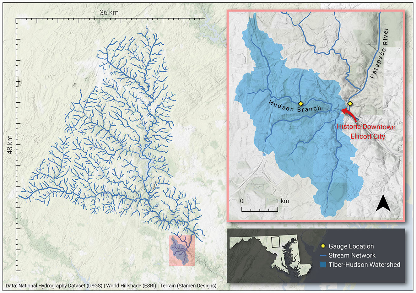
Figure 1. Ellicott City study domain. Left panel shows connected stream network that contributes to bottom-up flooding along the Patapsco River. Inset shows Tiber-Hudson with locations for Hudson Branch and Patapsco Ellicott stream gauges.
In response, Howard County identified a suite of flood management measures to reduce risks of future events. In total, 60 possible scenarios were evaluated, including the installation of new flood retention and diversion infrastructures, floodplain modification, building reclamation, and improved resilience measures (U.S. Army Corps of Engineers, 2019). As part of this comprehensive flood mitigation plan, additional effort has also been devoted to developing an operational flood forecast system for Ellicott City's historic downtown district.
The ability to forecast flash flooding is among the most challenging prospects in hydrometeorological research (Alfieri et al., 2011). Commonly used methods involve physical models, which attempt to capture rainfall-runoff dynamics using quantitative precipitation patterns, catchment characteristics, and stream morphology. However, these techniques are often computationally expensive and can be subject to stream-specific parameterization (Okuno et al., 2021). Numerous studies have outlined the advances in flash flood prediction as new techniques and datasets have been developed (Hapuarachchi et al., 2011; Gourley et al., 2014; Zanchetta and Coulibaly, 2020) yet in recent years, data-driven machine learning techniques have emerged as a promising approach to model flood conditions more efficiently and on smaller spatial scales.
“Machine learning” is a broad term that encompasses any number of algorithms that attempt to describe the relationship between input and output data (Choi et al., 2020). Unlike numerical or physical models, machine learning approaches can capture critical non-linearities in a hydrological system without explicit knowledge of the underlying geophysical processes (Mosavi et al., 2018). Certain types of models, known as artificial neural networks (ANN), have proven to be useful tools for time series problems like streamflow prediction and flood risk assessment (Alipour et al., 2020). Long short-term memory (LSTM) networks are a specific subset of ANNs that have broad applications for rainfall-runoff modeling, due to their ability to process and retain information from long sequences of data. Such frameworks that utilize multilayer neural networks to extract features from raw data are commonly referred to as “deep learning” (Shen et al., 2018).
Some of the most recent advances in hydrological deep learning come in the form of convolutional neural networks (CNN). Unlike LSTMs, CNNs are an emerging area of research which are designed to intake image data, allowing them to retain spatial dynamics that may be instructive to the problem of flash flood prediction (Shi et al., 2015). Landscape effects like soil moisture “memory” in the days following a rain event, for instance, can often impact the likelihood of a future flood event (McColl et al., 2017). Incorporating spatiotemporal inputs may therefore have important implications for flash flood prediction. This is particularly true for an area like Ellicott City, where current and forecasted stream conditions are used operationally to trigger emergency public alerts and evacuations.
Here, we introduce a hybrid Convolutional LSTM (ConvLSTM) model framework to evaluate how the addition of spatiotemporal data can potentially improve flash flood predictions in Ellicott City, Maryland. We use a simple LSTM as a baseline to predict future stage heights at the Hudson Branch stream gauge. We then benchmark this baseline against models driven by hydrometeorological inputs that can reflect the basin's specific landscape response. We evaluate both models for predictive accuracy, the ability to identify elevated stream conditions, and their performance in modeling the historical floods of 2016 and 2018. The following sections provide an overview of the study area and previous work in deep learning flood forecasting. Section 3 describes the details of data acquisition and processing, as well as the baseline and ConvLSTM model formulations. Sections 4 and 5 present the results and discussion, respectively. Finally, we discuss the specific applications of this model to operational flood management in Howard County and discuss caveats and future research needs.
2 Background and previous work
2.1 Ellicott City, Maryland
Ellicott City is a mill town founded in 1772, ~10 miles west of Baltimore. It is home to nearly 76,000 people and its downtown corridor was listed on the National Register of Historic Places in 1978 (National Park Service, 1978; U.S. Census Bureau, 2020). Throughout its history, the Ellicott City downtown corridor has endured numerous major floods due to its complex, and at times, unpredictable hydrology (The National Academies of Sciences, Engineering, and Medicine, 2020).
The city is situated at the confluence of several stream systems which can result in multiple flood mechanisms. The downtown area sits adjacent to the main stem of the Patapsco River. When flood waters from upstream cause the Patapsco to overtop, the city experiences “bottom-up” flooding (Halverson, 2019). The drainage basin feeding this system consists of nearly 50% developed land with a high degree of impervious surfaces (Maryland Department of Natural Resources, 2005). As a result, the basin is also prone to “top-down” floods, which occur when the Tiber River—which originates at higher elevations to the west of the city—overtops and flows downhill. The combination of steep terrain (~17° slope), shallow hydric soils, and large areas of exposed bedrock results in floodwaters being channeled directly through the downtown corridor's Main Street (The National Academies of Sciences, Engineering, and Medicine, 2020; Viterbo et al., 2020).
The specific hydrological characteristics of the Tiber-Hudson watershed make it one of the most volatile catchments in the nation. In a study of the flashiest watersheds in the contiguous United States (CONUS), two of the top 10 were found to be in the Baltimore area (Smith and Smith, 2015). A separate study by Saharia et al. (2016) developed a “flashiness” index, defined as the difference between the peak and action stage discharges, normalized by the flood response time and basin area (Saharia et al., 2016). Using this metric, the full study area would rank third in the state, while the smaller Tiber-Hudson watershed would have the highest average flashiness with an index of 0.952 out of 1 (Figure 2).
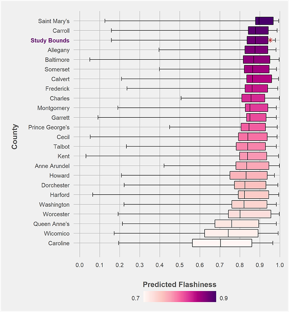
Figure 2. Distribution of flash flood severity (“flashiness”) of Maryland counties, based on data from Saharia et al. (2016). The area located strictly with this study's 36x48 kilometer domain is highlighted as the third highest average flashiness in the state, with the red star indicating the average flashiness of the smaller Tiber-Hudson watershed.
2.2 Deep learning for flood forecasting
Deep learning using neural networks has been an area of ongoing research in the hydrological sciences for decades (Daniel, 1991). In particular, LSTMs have been widely applied, due to their ability to solve the “vanishing gradient” problem present in earlier recurrent neural networks (RNN), in which the model training signal diminishes as it propagates through long sequences (Hochreiter and Schmidhuber, 1997; Shen, 2018). This is achieved through special structures within the LSTM cell that control which information is retained as training progresses (Figure 3A). At a given timestep, t, the model weights are updated based on a given input, xt, the previous cell output, ct−1, and the previous cell state, ht−1 (Rahman and Adjeroh, 2019). During the training process, the input gate, it, controls which inputs should be remembered, while the forget gate, ft, determines which past state memory should be discarded and which should be sent on to the output gate, ot (Shen, 2018). Numerous studies have recently demonstrated how LSTM networks can improve performance relative to other physically-based hydrological models (Kratzert et al., 2018; Xiang et al., 2020; Li et al., 2021).
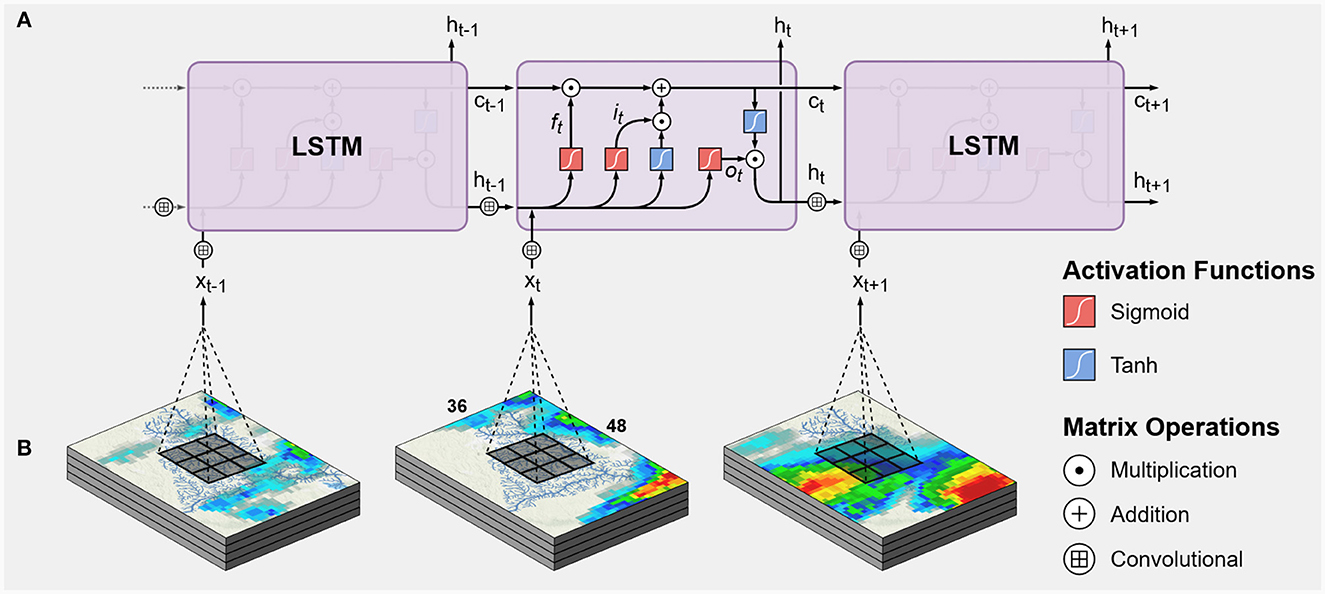
Figure 3. (A) Schematic of basic LSTM cell, (B) Addition of convolutional structures to produce ConvLSTM cell. Inputs and previous hidden states are convolved using 3x3 kernel to produce 3-dimensional tensors which pass through network. Figure adapted from Rahman and Adjeroh (2019).
Contrasted with LSTMs, convolutional neural networks can process data hierarchically in the form of arrays, making them better suited to image or video classification (LeCun et al., 2015). Recent studies have demonstrated the applicability of CNNs to flood susceptibility and extent mapping (Gebrehiwot et al., 2019; Wang et al., 2020), extreme weather detection (Liu et al., 2016), and forecasted precipitation estimation (Sadeghi et al., 2019). In a demonstration on deep learning for precipitation nowcasting, Shi et al. (2015) proposed a hybrid approach, ConvLSTM, which replaces matrix multiplication with convolutional operators for both the input and state-to-state transitions (Figure 3B; Shi et al., 2015). This hybrid approach has proven to outperform other neural network frameworks in studies ranging from precipitation nowcasting (Kim et al., 2017; Weyn et al., 2019; Kumar et al., 2020; Gamboa-Villafruela et al., 2021), to soil moisture prediction (ElSaadani et al., 2021), to flood extent mapping (Ulloa et al., 2022).
While ConvLSTM models have been shown to be effective at several hydrometeorological applications, there is less research applying these types of models directly to streamflow or stage forecasts. Moishin et al. (2021) developed a flood forecasting model based on a Flood Index (IF) derived from daily rainfall across nine sites in Fiji (Moishin et al., 2021). While the ConvLSTM model performed best in forecasting daily stream conditions, the authors note the analysis was limited by only using two input features and would benefit from hourly observations. Ha et al. (2021) also presents a ConvLSTM-based flood forecasting model using monthly streamflow data and an El Niño–Southern Oscillation (ENSO) index as inputs (Ha et al., 2021). Here, the individual datasets were 1-dimensional but were grouped into 2-dimensional inputs for model training. While both studies have advanced the state-of-the-art in operational flood forecast modeling, neither explicitly utilizes spatially-distributed inputs or addresses the specific issue of flash flooding.
2.3 Flood forecasting in Ellicott City
Efforts to monitor flood conditions within Ellicott City rely on observations of current stage heights, discharge, and forecasted precipitation. The Howard County Stormwater Management Division (SWMD) monitors these real-time conditions using an internal web platform, OneRain, which visualizes data from municipal and federal gauges. SWMD has established several stage thresholds (Significant, Warning, and Alarm) which use observed conditions to trigger subsequent flood mitigation measures. Until recently, the system was unable to forecast future flood conditions in real-time.
Initial attempts to integrate real-time stage forecasts into this web platform have shown promising results. Early implementations focused on generating statistical forecasts using autoregressive (AR) and autoregressive integrated moving average (ARIMA) models. These models were driven by times series of upstream discharge and area-averaged soil moisture and precipitation data from the North American Land Data Assimilation System (NLDAS). A subsequent implementation compared these statistical forecasts to those generated by a many-to-one LSTM and added in-situ precipitation observations. The current OneRain platform features a sequence-to-sequence encoder/decoder LSTM that forecasts operational stage height predictions up to 8-h out (see Supplementary Figure 1). This web interface supports two separate forecast models: one that relies solely on previous gauge observations and one which incorporates point estimates of forecasted precipitation from the National Oceanic and Atmospheric Administration (NOAA) High-Resolution Rapid Refresh (HRRR) product (Dowell et al., 2022).
These initial models have demonstrated high accuracy when predicting across the validation datasets, incurring a root mean square error (RMSE) of 0.07 feet. However, when evaluating performance for the elevated flood conditions, the models demonstrate much higher errors (RMSE = 0.85), indicating only a moderate ability to forecast flash flood conditions. The results of the initial model implementations are summarized in Supplementary Table 1 and are contrasted with the results of this analysis in the Discussion section. As these stage thresholds are critical to the flood mitigation practices within SWMD, additional research is needed to improve predictive accuracy in Ellicott City.
3 Materials and methods
3.1 Baseline model: LSTM
A baseline model was constructed using a simple implementation of an LSTM with a global attention mechanism (Luong et al., 2015; Rémy, 2017). Attention mechanisms are used to help identify relevant information in long sequences of data by drawing global dependencies between input and response variables (Vaswani et al., 2017). Data inputs for the baseline model are stage height observations at previous timesteps at both the Hudson Branch and Patapsco Ellicott gauge locations (Table 1). Time series of stream observations with varying input windows (1, 2, 3, 4, 6, and 8 h) were used to predict stage height at time n+1. Stream observations from January 2016 through October 2020 were acquired from OneRain and resampled to align to hourly indices for a total of 42,384 samples (2016-01-01 00:00 through 2020-10-31 23:00). The baseline model was trained on data 70% of the data, from January 2016 through May 2019. It should be noted that this training period contained both the 2016 and 2018 flood events. A diagnostic test was performed which split the 2016 and 2018 floods into the training and validation sets which resulted in a 52% increase in RMSE when forecasting elevated flood conditions. Models were validated against the remaining 30% of data, from May 2019 through October 2020. The full configuration parameters for the baseline LSTM can be seen in Table 2.

Table 1. Data inputs for baseline (LSTM) and ConvLSTM models.
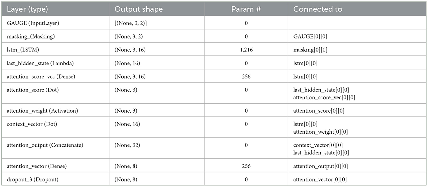
Table 2. Configuration parameters for the baseline LSTM with global attention mechanism.
3.2 ConvLSTM model
3.2.1 Study domain
The performance of the baseline LSTM is compared against model formulations which include the addition of spatiotemporal data inputs. The spatial domain for this study was determined using the U.S. Geological Survey's (USGS) National Hydrography Datasets Plus (NHDPlus) High Resolution dataset (Moore et al., 2019). A stream network analysis was performed using QGIS to determine the connected channels upstream of Ellicott City. A 36x48 km grid with 1-km horizontal resolution was superimposed on this stream network to establish a study area that could capture the potential for top-down and bottom-up flood mechanisms (Figure 1).
3.2.2 Data selection and processing
Four spatiotemporal datasets were selected for their temporal resolution (minimum of hourly measurements), moderate spatial resolution, and applicability for rainfall-runoff modeling (Table 1). Remotely-sensed precipitation data from the National Aeronautics and Space Administration (NASA) Global Precipitation Measurement (GPM) mission was acquired using the Integrated Multi-satellitE Retrievals for GPM (IMERG) algorithm.
Soil moisture data from the NLDAS Noah Land Surface Model (LSM) was acquired through the Goddard Earth Sciences Data and Information Services Center (GESDISC; Xia et al., 2012a,b).
Base reflectivity from NOAA's Next Generation Radar (NEXRAD) was acquired as a mosaicked product through Iowa State University's Iowa Environmental Mesonet. NEXRAD Level III 1-h accumulated rainfall data was acquired from Google Cloud public data repositories. Level III radar observations from the Sterling, Virginia KLWX doppler station were converted from radial to grid format using the Python ARM Radar Toolkit (Helmus and Collis, 2016).
All datasets were temporally subsetted to the closest hour to match the hourly indices of the gauged response data. The NEXRAD Mosaic, Noah LSM, and GPM IMERG data are available at CONUS scales and at regular intervals while the KLWX data contained several timesteps with no available data. The timesteps for the missing KLWX data (n = 1,405) were processed using masked arrays during the training process. All datasets were then spatially resampled to 1-km horizontal resolution using the “Nearest Neighbor” method in QGIS to align to the 36x48 kilometer study domain grid.
3.2.3 ConvLSTM model architecture
ConvLSTM models were constructed using a multi-headed architecture, where each spatiotemporal data input is processed as a separate neural network “head.” The output of each ConvLSTM head is then merged and concatenated with the baseline LSTM to produce a single output for the stream stage response variable (Kaushik et al., 2020). This model structure is designed to train each input more efficiently and help quantify the marginal effects of including additional spatiotemporal data as predictors. Model architecture was tuned for dropout rate, learning rate, and activation function using a hyperparameter grid search. Training and validation were performed using different combinations of spatial inputs, resulting in the evaluation of 15 separate ConvLSTM model versions (Table 3). A network diagram of the full model with all spatiotemporal inputs (version 15) included can be seen in Figure 4. Here, all four hydrometeorological inputs are processed using the Keras ConvLSTM2D and Conv3D hidden layers with the Rectified Linear Unit (ReLU) activation function before being concatenated with the baseline LSTM. Each version was trained using the same varying input windows as described in the baseline model.
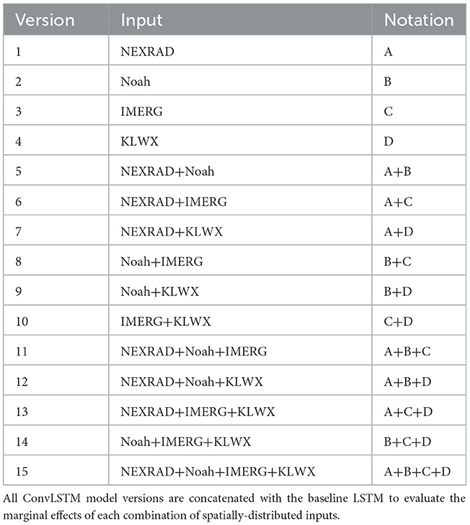
Table 3. Data input combinations for ConvLSTM models.
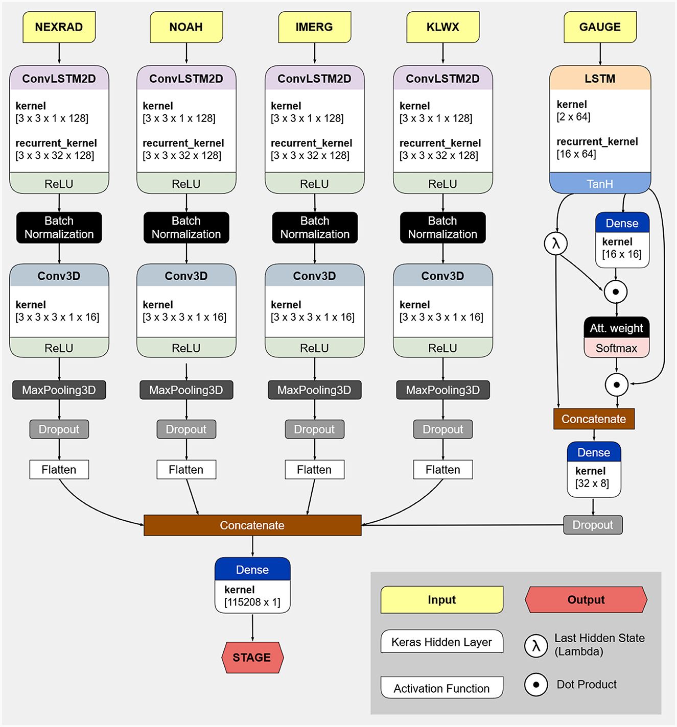
Figure 4. Example of full network architecture with all spatiotemporal inputs (Version 15; Table 3) concatenated with LSTM with global attention mechanism.
Both the Baseline LSTM and ConvLSTM neural networks were constructed using the open-source Keras library for Python with the TensorFlow backend, developed by Google (Abadi et al., 2015; Chollet, 2015). All models were trained for 100 epochs on the NASA Center for Climate Simulation (NCCS) machine learning cluster using NVIDIA V100 GPUs. Training and validation for each version were repeated 5 times to account for randomized initialization conditions, resulting in a total of 480 different model runs.
3.3 Problem objectives
We evaluate model performance as the ability to accurately predict observed stage height at time t+1 by seeking to minimize RMSE:
where yi and ŷi are the observed and estimated stage heights, respectively, at the Hudson Branch gauge site.
Model accuracy was evaluated for the full validation set (May 2019 to October 2020), as well as for the historical 2016 and 2018 flood events. Statistical t-tests were used to determine if mean RMSE values for each model version differed significantly from the baseline LSTM for each input window (p < 0.05).
In addition to overall accuracy, we consider each model's ability to detect elevated flood conditions using a specified threshold. Based on the full observational record from OneRain, we identify a threshold stage height of 254.32 feet using the find_peaks function within Python's SciPy library and a statistical prominence of 0.75 (Figure 5). This height is ~1 foot below the “Significant” level established by the Howard County SWM for the Hudson Branch site. Timesteps with stage heights above this threshold are considered “peak indices” (n = 164) and the accuracy at these timesteps is evaluated as a separate model objective.
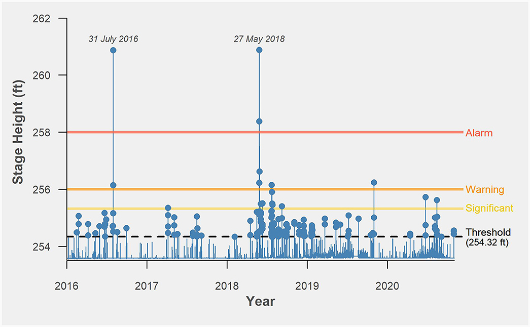
Figure 5. Identification of “peak indices” at the Hudson Branch stream gauge using statistical prominence approach.
4 Results
4.1 Validation accuracy
When evaluating accuracy over the full validation set, the inclusion of spatiotemporal data generally led to improved predictions over the baseline LSTM (see Supplementary Figure 2). Model version 15 (all spatial inputs) produced the lowest average RMSE (0.069), though none of the values using the 1-h input window were found to be statistically significant. Model performance varies depending on which input combinations were used, with some general trends emerging. Model formulations using shorter input windows tended to produce lower RMSE than those which included more hours of data. That said, larger input windows (4+ h) were more likely to produce statistically significant improvements over their respective baselines. Model versions featuring Noah soil moisture (B) and KLWX accumulated rainfall (D)—either individually or in combination—tended to result in the lowest, statistically significant errors. A hydrograph view also shows that the model with the lowest average error (version 15, 1-h) appears to capture daily and seasonal trends yet fails to capture the magnitude of larger peaks when predicting on unseen data (Figure 6).
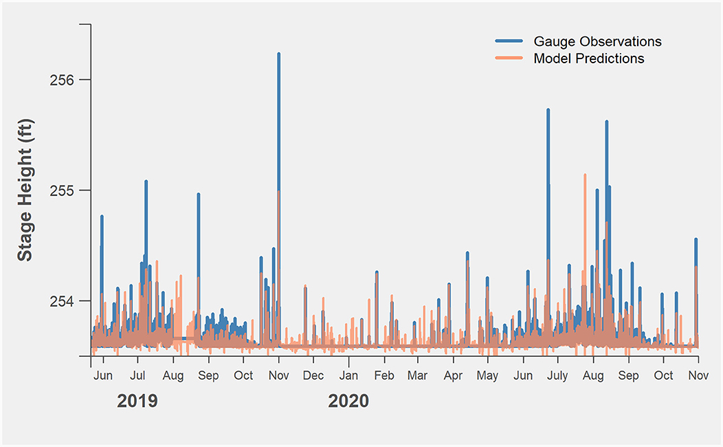
Figure 6. Predicted vs. observed stage heights at Hudson Branch for the full validation set.
4.2 Peak index accuracy
Isolating the prediction error for just the peak indices more clearly reveals the model improvements when incorporating spatial information (Figure 7). Here too, ConvLSTM version 15 using a 1-h window produces the lowest RMSE, yet in this case the improvement was found to be statistically significant. The majority of ConvLSTM model formulations resulted in lower errors compared to the baseline LSTM of their respective window, with a few exceptions. The models using a 3-h input window generally performed worse than the same formulations with either a 2- or 4-h window. Similar to the results in the full validation set, certain input combinations resulted in increased predictive accuracy, though those trends are less consistent.

Figure 7. Heatmap of RMSE for predicted stage height at specified “peak indices.” Lower values indicate higher accuracy. Asterisks denote model versions that were found to have statistically significant differences in mean RMSE relative to baseline LSTM (p < 0.05).
When simply comparing the models' ability to successfully predict peak indices, the ConvLSTM version 15 also outperforms the baseline LSTM. A confusion matrix for both shows that the ConvLSTM correctly predicted an average of two additional flood peaks compared to the baseline model, though both formulations exhibited high degrees of false negatives (Supplementary Figure 3).
4.3 Historical flood performance
Evaluating the trained model over the historical data shows its ability to capture the events from 2016 and 2018. Figure 8 shows a hydrograph of the model version with the lowest average RMSE in predicting these historical floods. For the 2016 Flood, this was achieved using version 12 (NEXRAD + Noah + KLWX) with an input window of 6-h. Despite this version achieving the lowest error, a general trend shows that a 3-h input window across all model versions appears to be the most instructive for that event (Supplementary Figures 4, 5).
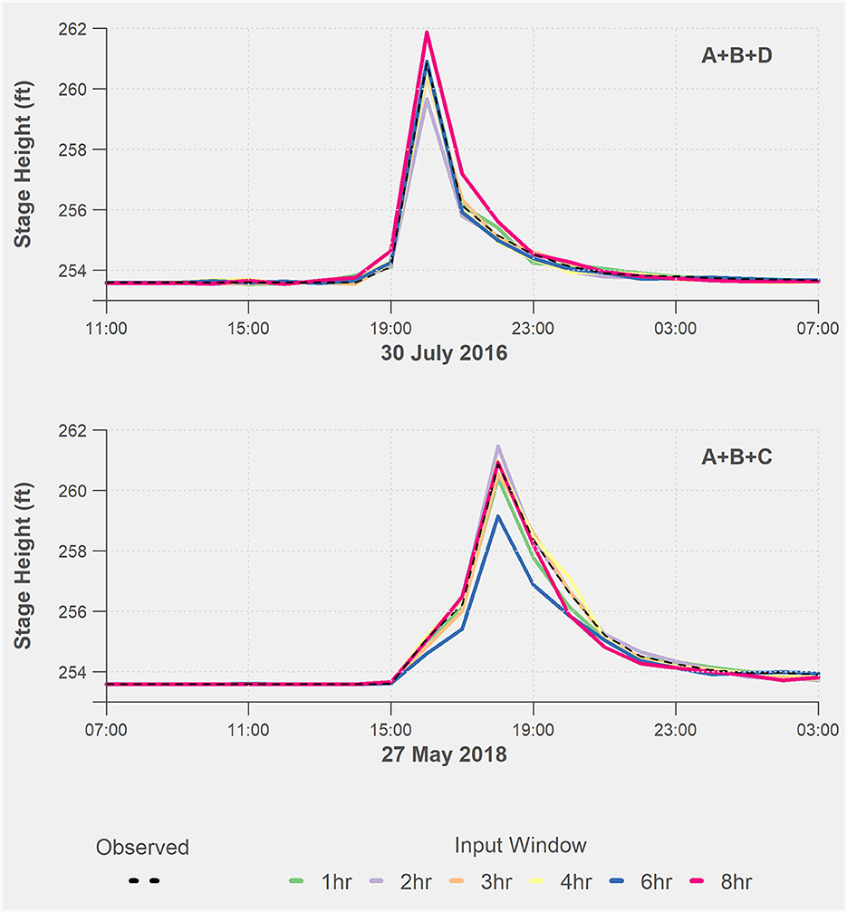
Figure 8. Observed vs. predicted stage heights for best performing model versions for 2016 (top) and 2018 (bottom) floods. Color bars represent model runs for different input windows. Dashed line indicates observations from OneRain gauge network.
For the 2018 Flood, version 11 (NEXRAD + IMERG + Noah) with a 1-h window achieved the highest accuracy. The performance of all versions can be seen in Supplementary Figures 6, 7. The 2018 Flood showed similar variability to the 2016 event. For both historical floods, a number of the ConvLSTM models were not found to have statistically better performance relative to the LSTM baseline. However, those that did showed more dramatic improvements than the marginal gains achieved in either the full validation or the peak index results. Both the 2016 and 2018 floods also displayed similar trends for model versions that performed worse than the baseline. In particular, versions featuring Noah soil moisture (B) and IMERG precipitation (C) resulted in some RMSE that were more than double that of the baseline.
5 Discussion and conclusions
We explored how the inclusion of spatiotemporal inputs can improve the predictive performance of a data-driven flood forecasting model. Overall, we find that the ConvLSTM models often outperform the baseline LSTM, though the relative improvements differ according to the objective in question. When evaluating total accuracy over the full validation data, the ConvLSTM model with all available inputs (version 15) achieves the lowest average error. The hydrograph view (Figure 6) suggests that this comparatively lower error maybe due to the model's ability to accurately predict the daily and seasonal fluctuations that comprise the bulk of the training data. This trend is most pronounced at timesteps where observed stage heights were below the peak threshold value, particularly during the drier winter months. Conversely, model errors appear systematically larger when predicting higher, more extreme stream stages.
These results are consistent with previous studies on hydrological prediction of extreme events. Frame et al. (2022) demonstrated that across multiple data-driven and process-based models, prediction error increased with event magnitude. It is likely that the comparatively small number of peak events available for training contributed to the model's poor performance on the validation set, which is a common challenge when predicting extreme events (Qi and Majda, 2020).
Despite not capturing the magnitudes of some of the larger stage heights, model version 15 also performs best on the “peak index” accuracy metric. Contrasted with the full validation set, more of the model versions evaluated for these peak indices were found to produce larger, statistically significant improvements over the baseline LSTM. Using a 1-h input window the addition of spatiotemporal inputs resulted in a ~26% improvement to the model, yet exhibited only a 6% improvement at correctly identifying peak indices. The high degree of type II error (i.e., false negatives) for both the ConvLSTM and baseline models, however, still reflects an increased need for predictive power at detecting elevated flood conditions in general.
The broader performance trends across all model formulations differ depending on which objective is being considered. When evaluating for peak indices or the full validation data, most model versions appear to benefit from a shorter input window. This finding runs counter to what may be expected in a data-driven model, where additional information about prior conditions typically leads to improved performance. One possible explanation could be found in the highly-flashy nature of this particular catchment. The rainfall-runoff response time in the Tiber-Hudson watershed is incredibly rapid, and so larger input windows may offer diminishing returns in predictive ability. Increased granularity could be achieved using sub-hourly gauge observations (which are available through OneRain) however the limiting factor is currently higher-frequency satellite observations. It's also possible that additional information about land surface features, such as elevation or land use/land cover would help to inform how the rainfall-runoff response propagates through the catchment.
Despite the floods of 2016 and 2018 occurring through similar top-down mechanisms, the model results reveal different characteristics for each event. The 2016 storm shows a strong preference for models using 3-h input window that isn't present in the 2018 event. Both storms produced similar amounts of rainfall (6.60 vs. 6.56 inches in 2016 and 2018, respectively). However, while both storms had ~3-h durations, the 2016 precipitation was introduced in a single downpour while 2018 had two distinct intervals of heavy rainfall (Doheny and Nealen, 2021). It's possible the differences in the evolution of these events can account for their respective model performance.
When viewing the contribution of specific datasets, certain inputs like the IMERG precipitation and Noah soil moisture appear to perform poorly individually, yet when paired with additional radar datasets often produce the best predictions for the historical floods. The higher errors of these individual inputs are likely due to their comparatively coarser resolution; IMERG and Noah are produced at 0.1- and 0.125-degree horizontal resolution (~11–12-km), while both NEXRAD products are processed at closer to 1-km horizontal resolution. So, while they are resampled to match the domain grid, these inputs may not contain enough spatial information to be as instructive on their own.
6 Caveats and future research needs
The results explored here reflect the specific hydrological characteristics of a single, highly-flashy watershed, as well as the targeted applied science needs of flood managers in Howard County. While some of the improvements demonstrated here may appear small, they can still potentially have important implications when planning for flash flood events. This is especially true for improvements made to peak index prediction, as these events factor most heavily into their risk reduction operations.
As is true with any data-driven approach, the framework presented here is envisaged to continue to improve as more training information and potential inputs become available. Additional datasets such as landcover or time series from upstream gauges could be incorporated to provide additional predictive accuracy, particularly if they are available in near real-time. Future plans to expand this methodology will focus on other stream reaches within the Howard County gauge network. Additionally, it will be critical to validate the model on other similarly flashy watersheds to assess the generalizability of this approach for flash flood forecasting.
While deep learning approaches like ConvLSTM can offer certain advantages, it is helpful to benchmark against established physical alternatives. NOAA's National Water Model (NWM) produces high-resolution streamflow forecasts over CONUS. A recent study by Viterbo et al. (2020) demonstrated how NWM forecasts were skillful in capturing trends from the 2018 Ellicott City Flood (Viterbo et al., 2020). However, the authors caution that the NWM likely underestimates streamflow in the small Ellicott City basin and note the difficulty in applying a CONUS-scale to highly-localized events. A comparison of the OneRain gauge observations to the NWM Reanalysis 2.0 model confirms that streamflow was indeed under-predicted at the Hudson Gauge site for both the 2016 and 2018 Floods (see Supplementary Figure 8).
Much of the power of machine learning methods comes from their ability to uncover non-linear relationships between inputs and outputs without explicit representations of a specific catchment. This can be especially useful when evaluating small and uncalibrated basins. Kratzert et al. (2019) showed that a LSTM network performed better at predicting streamflow on ungauged basins than process-based models calibrated on gauged basins. Ellicott City, due to its highly flashy watershed and long history of flooding, provides an ideal backdrop for exploring such a difficult flood management problem.
Data availability statement
The raw data supporting the conclusions of this article will be made available by the authors, without undue reservation.
Author contributions
PO: Data curation, Formal analysis, Investigation, Methodology, Software, Validation, Visualization, Writing—original draft. JB: Conceptualization, Funding acquisition, Methodology, Project administration, Supervision, Writing—review & editing. SK: Conceptualization, Funding acquisition, Methodology, Project administration, Supervision, Writing—review & editing. BC: Methodology, Resources, Supervision, Writing—review & editing.
Funding
The author(s) declare that no financial support was received for the research, authorship, and/or publication of this article.
Acknowledgments
The authors sincerely thank Manabendra Saharia for providing the raw data to produce the analysis on Flashiness in Maryland Counties. Additional thanks are given to members of the NASA DEVELOP Program who contributed to previous iterations of this research: Scott Cunningham, Jonathan Donesky, Terra Edenhart-Pepe, Darcy Gray, Ryan Hammock, Erika Munshi, Eli Orland, Julio Peredo, Matthew Pruett, Caroline Resor, Alina Schulz, and Callum Wayman.
Conflict of interest
PO was employed by Science Systems and Applications, Inc. for the period this research was conducted.
The authors declare that the research was conducted in the absence of any commercial or financial relationships that could be construed as a potential conflict of interest
Publisher's note
All claims expressed in this article are solely those of the authors and do not necessarily represent those of their affiliated organizations, or those of the publisher, the editors and the reviewers. Any product that may be evaluated in this article, or claim that may be made by its manufacturer, is not guaranteed or endorsed by the publisher.
Supplementary material
The Supplementary Material for this article can be found online at: https://www.frontiersin.org/articles/10.3389/frwa.2024.1346104/full#supplementary-material
Abbreviations
ANN, Artificial neural network; ARIMA, Autoregressive Integrated Moving Average; CNN, Convolutional neural network; CONUS, Continental United States; ConvLSTM, Convolutional long short-term memory; GESDISC, Goddard Earth Sciences Data and Information Services Center; GPM, Global Precipitation Measurement; HRRR, High-Resolution Rapid Refresh; IMERG, Integrated Multi-satellitE Retrievals for GPM; KLWX, Sterling, Virginia Doppler radar site; LSM, Land surface model; LSTM, Long short-term memory; NEXRAD, Next Generation Radar; NLDAS, North American Land Data Assimilation System; NWM, National Water Model; RMSE, Root-mean-square error; RNN, Recurrent neural network; SWMD, Howard County Stormwater Management Division.
References
Abadi, M., Agarwal, A., Barham, P., Brevdo, E., Chen, Z., Citro, C., et al. (2015). TensorFlow: Large-Scale Machine Learning on Heterogeneous Systems. Available online at: https://www.tensorflow.org/about/bib
Alfieri, L., Velasco, D., and Thielen, J. (2011). Flash flood detection through a multi-stage probabilistic warning system for heavy precipitation events. Adv. Geosci. 29, 69–75. doi: 10.5194/adgeo-29-69-2011
Alipour, A., Ahmadalipour, A., Abbaszadeh, P., and Moradkhani, H. (2020). Leveraging machine learning for predicting flash flood damage in the Southeast US. Environ. Res. Lett. 15:e024011. doi: 10.1088/1748-9326/ab6edd
Ashley, S. T., and Ashley, W. S. (2008). Flood fatalities in the United States. J. Appl. Meteorol. Climatol. 47, 805–818. doi: 10.1175/2007JAMC1611.1
Choi, R. Y., Coyner, A. S., Kalpathy-Cramer, J., Chiang, M. F., and Campbell, J. P. (2020). Introduction to machine learning, neural networks, and deep learning. Transl. Vis. Sci. Technol. 9:14. doi: 10.1167/tvst/9.2.14
Chollet, F. (2015). Keras: Deep Learning Library for Theano and Tensorflow. Available online at: https://keras.io/getting_started/faq/#how-should-i-cite-keras
Clinch, R. (2016). The Economic Impact of the 2016 Ellicott City Flood. University of Baltimore. Available online at: http://www.jacob-france-institute.org/wp-content/uploads/Economic-Impact-Ellicott-City-Flood-2016.pdf (accessed April 23, 2020).
Creutin, J. D., Borga, M., Lutoff, C., Scolobig, A., Ruin, I., and Créton-Cazanave, L. (2009). Catchment dynamics and social response during flash floods: the potential of radar rainfall monitoring for warning procedures. Meteorol. Appl. J. Forecast. Pract. Appl. Train. Tech. Model. 16, 115–125. doi: 10.1002/met.128
Daniel, T. M. (1991). “Neural networks-applications in hydrology and water resources engineering,” in Proc., Int. Hydrol. and Water Resour. Symp. (Perth, WA: Institution of Engineers).
Davenport, F. V., Burke, M., and Diffenbaugh, N. S. (2021). Contribution of historical precipitation change to US flood damages. Proc. Natl. Acad. Sci. U. S. A. 118:1752. doi: 10.1073/pnas.2017524118
Doheny, E. J., and Nealen, C. W. (2021). Storms and floods of July 30, 2016, and May 27, 2018, in Ellicott City, Howard County, Maryland. US Geol. Survey 2021:3025. doi: 10.3133/fs20213025
Dowell, D. C., Alexander, C. R., James, E. P., Weygandt, S. S., Benjamin, S. G., Manikin, G. S., et al. (2022). The high-resolution rapid refresh (HRRR): an hourly updating convection-allowing forecast model. Motivat. Syst. Descript. 37, 1371–1395. doi: 10.1175/WAF-D-21-0151.1
ElSaadani, M., Habib, E., Abdelhameed, A. M., and Bayoumi, M. (2021). Assessment of a spatiotemporal deep learning approach for soil moisture prediction and filling the gaps in between soil moisture observations. Front. Artif. Intell. 4:636234. doi: 10.3389/frai.2021.636234
Frame, J. M., Kratzert, F., Klotz, D., Gauch, M., Shalev, G., Gilon, O., et al. (2022). Deep learning rainfall–runoff predictions of extreme events. Hydrol. Earth Syst. Sci. 26, 3377–3392. doi: 10.5194/hess-26-3377-2022
Gamboa-Villafruela, C. J., Fernández-Alvarez, J. C., Márquez-Mijares, M., Pérez-Alarcón, A., and Batista-Leyva, A. J. (2021). Convolutional LSTM architecture for precipitation nowcasting using satellite data. Environ. Sci. Proc. 8:33. doi: 10.3390/ecas2021-10340
Gebrehiwot, A., Hashemi-Beni, L., Thompson, G., Kordjamshidi, P., and Langan, T. E. (2019). Deep convolutional neural network for flood extent mapping using unmanned aerial vehicles data. Sensors 19:1486. doi: 10.3390/s19071486
Gourley, J. J., Flamig, Z. L., Hong, Y., and Howard, K. W. (2014). Evaluation of past, present and future tools for radar-based flash-flood prediction in the USA. Hydrol. Sci. J. 59, 1377–1389. doi: 10.1080/02626667.2014.919391
Ha, S., Liu, D., and Mu, L. (2021). Prediction of Yangtze River streamflow based on deep learning neural network with El Niño–Southern Oscillation. Sci. Rep. 11, 1–23. doi: 10.1038/s41598-021-90964-3
Halverson, J. B. (2019). Flood City, USA: Ellicott City faces latest historical flooding. Weatherwise 72, 12–18. doi: 10.1080/00431672.2019.1559267
Hapuarachchi, H. P., Wang, Q. J., and Pagano, T. C. (2011). A review of advances in flash flood forecasting. Hydrol. Process. 25, 2771–2784. doi: 10.1002/hyp.8040
Helmus, J. J., and Collis, S. M. (2016). The Python ARM Radar Toolkit (Py-ART), a library for working with weather radar data in the python programming language. J. Open Res. Softw. 4:e25. doi: 10.5334/jors.119
Hochreiter, S., and Schmidhuber, J. (1997). Long short-term memory. Neural Comput. 9, 1735–1780. doi: 10.1162/neco.1997.9.8.1735
Kaushik, S., Choudhury, A., Dasgupta, N., Natarajan, S., Pickett, L. A., and Dutt, V. (2020). “Ensemble of multi-headed machine learning architectures for time-series forecasting of healthcare expenditures,” in Applications of Machine Learning Algorithms for Intelligent Systems, eds. P. Johri, J. K. Verma, and S. Paul (Singapore: Springer), 205.
Kim, S., Hong, S., Joh, M., and Song, S. K. (2017). Deeprain: Convlstm network for precipitation prediction using multichannel radar data. arXiv [Preprint]. arXiv:1711.02316.
Kratzert, F., Klotz, D., Brenner, C., Schulz, K., and Herrnegger, M. (2018). Rainfall–runoff modelling using Long Short-Term Memory (LSTM) networks. Hydrol. Earth Syst. Sci. 22, 6005–6022. doi: 10.5194/hess-22-6005-2018
Kratzert, F., Klotz, D., Herrnegger, M., Sampson, A. K., Hochreiter, S., and Nearing, G. S. (2019). Toward improved predictions in ungauged basins: exploiting the power of machine learning. Water Resour. Res. 55, 11344–11354. doi: 10.1029/2019WR026065
Kumar, A., Islam, T., Sekimoto, Y., Mattmann, C., and Wilson, B. (2020). Convcast: an embedded convolutional LSTM based architecture for precipitation nowcasting using satellite data. PLoS ONE 15:e0230114. doi: 10.1371/journal.pone.0230114
LeCun, Y., Bengio, Y., and Hinton, G. (2015). Deep learning. Nature 521, 436–444. doi: 10.1038/nature14539
Li, W., Kiaghadi, A., and Dawson, C. (2021). High temporal resolution rainfall–runoff modeling using long-short-term-memory (LSTM) networks. Neural Comput. Appl. 33, 1261–1278. doi: 10.1007/s00521-020-05010-6
Liu, Y., Racah, E., Prabhat, A., Correa, J., Khosrowshahi, A., Lavers, D., et al. (2016). Application of Deep Convolutional Neural Networks for Detecting Extreme Weather in Climate Datasets. ArXiv Prepr. Available online at: https://arxiv.org/abs/1605.01156v1 (accessed April 10, 2020).
Luong, M.-T., Pham, H., and Manning, C. D. (2015). Effective approaches to attention-based neural machine translation. ArXiv Prepr. ArXiv150804025. doi: 10.18653/v1/D15-1166
Maryland Department of Natural Resources (2005). Characterization of the Patapsco River lower north branch watershed in Howard County, Maryland. Maryland Department of Natural Resources. Available online at: https://dnr.maryland.gov/waters/Documents/WRAS/patlnb_char.pdf (accessed August 11, 2021).
McColl, K. A., Alemohammad, S. H., Akbar, R., Konings, A. G., Yueh, S., and Entekhabi, D. (2017). The global distribution and dynamics of surface soil moisture. Nat. Geosci. 10, 100–104. doi: 10.1038/ngeo2868
Moishin, M., Deo, R. C., Prasad, R., Raj, N., and Abdulla, S. (2021). Designing deep-based learning flood forecast model with ConvLSTM hybrid algorithm. IEEE Access 9, 50982–50993. doi: 10.1109/ACCESS.2021.3065939
Moore, R. B., McKay, L. D., Rea, A. H., Bondelid, T. R., Price, C. V., Dewald, T. G., et al. (2019). User's Guide for the National Hydrography Dataset Plus (NHDPlus) High Resolution. Reston, VA: U.S. Geological Survey. Available online at: http://pubs.er.usgs.gov/publication/ofr20191096
Mosavi, A., Ozturk, P., and Chau, K. (2018). Flood prediction using machine learning models: literature review. Water 10:1536. doi: 10.3390/w10111536
National Park Service (1978). Ellicott City Historic District. Natl. Regist. Hist. Places. Available online at: https://npgallery.nps.gov/NRHP/AssetDetail?assetID=a96e0078-fcb9-40d0-abb7-5467cc6564a9 (accessed August 9, 2021).
Okuno, S., Ikeuchi, K., and Aihara, K. (2021). Practical data-driven flood forecasting based on dynamical systems theory. Water Resour. Res. 57:e2020WR028427. doi: 10.1029/2020WR028427
Qi, D., and Majda, A. J. (2020). Using machine learning to predict extreme events in complex systems. Proc. Natl. Acad. Sci. U. S. A. 117, 52–59. doi: 10.1073/pnas.1917285117
Rahman, S. A., and Adjeroh, D. A. (2019). Deep learning using convolutional LSTM estimates biological age from physical activity. Sci. Rep. 9, 1–15. doi: 10.1038/s41598-019-46850-0
Rémy, P. (2017). Keras Attention Mechanism. Available online at: https://github.com/philipperemy/keras-attention-mechanism (accessed August 11, 2021).
Sadeghi, M., Asanjan, A. A., Faridzad, M., Nguyen, P., Hsu, K., Sorooshian, S., et al. (2019). PERSIANN-CNN: precipitation estimation from remotely sensed information using artificial neural networks–convolutional neural networks. J. Hydrometeorol. 20, 2273–2289. doi: 10.1175/JHM-D-19-0110.1
Saharia, M., Kirstetter, P.-E., Vergara, H., Gourley, J. J., Hong, Y., and Giroud, M. (2016). Mapping flash flood severity in the United States. J. Hydrometeorol. 18, 397–411. doi: 10.1175/JHM-D-16-0082.1
Shen, C. (2018). A transdisciplinary review of deep learning research and its relevance for water resources scientists. Water Resour. Res. 54, 8558–8593. doi: 10.1029/2018WR022643
Shen, C., Laloy, E., Elshorbagy, A., Albert, A., Bales, J., Chang, F.-J., et al. (2018). HESS Opinions: incubating deep-learning-powered hydrologic science advances as a community. Hydrol. Earth Syst. Sci. 22, 5639–5656. doi: 10.5194/hess-22-5639-2018
Shi, X., Chen, Z., Wang, H., Yeung, D.-Y., Wong, W., and WOO, W. (2015). “Convolutional LSTM network: a machine learning approach for precipitation nowcasting,” in Advances in Neural Information Processing Systems, eds C. Cortes, N. Lawrence, D. Lee, M. Sugiyama, and R. Garnett (Curran Associates, Inc.). Available online at: https://proceedings.neurips.cc/paper_files/paper/2015/file/07563a3fe3bbe7e3ba84431ad9d055af-Paper.pdf
Smith, B. K., and Smith, J. A. (2015). The flashiest watersheds in the contiguous United States. J. Hydrometeorol. 16, 2365–2381. doi: 10.1175/JHM-D-14-0217.1
Špitalar, M., Gourley, J. J., Lutoff, C., Kirstetter, P.-E., Brilly, M., and Carr, N. (2014). Analysis of flash flood parameters and human impacts in the US from 2006 to 2012. J. Hydrol. 519, 863–870. doi: 10.1016/j.jhydrol.2014.07.004
The National Academies of Sciences Engineering, and Medicine. (2020). Community Engagement for Flood Mitigation: Ellicott, City MD Case Study. The National Academies of Sciences Engineering, and Medicine. Available online at: https://www.preservationmaryland.org/wp-content/uploads/2020/03/Resilient-America-Ellicott-City-Case-Study-Mar2020-FINAL.pdf (accessed August 12, 2020).
U.S. Army Corps of Engineers (2019). Evaluation of Ellicott City Flood Risk Management Alternatives. Howard County, Maryland. Available online at: https://f7ffdcab-43e5-473c-85ed-f1db9af7ab7a.filesusr.com/ugd/34b2b4_750c08122d734b10abeaff470f9248fa.pdf (accessed August 10, 2021).
U.S. Census Bureau (2020). QuickFacts: Ellicott City CDP, Maryland. Available online at: https://www.census.gov/quickfacts/fact/table/ellicottcitycdpmaryland/POP010220#POP010220 (accessed August 9, 2021).
Ulloa, N. I., Yun, S.-H., Chiang, S.-H., and Furuta, R. (2022). Sentinel-1 spatiotemporal simulation using convolutional LSTM for flood mapping. Remote Sens. 14:246. doi: 10.3390/rs,14020246
Vaswani, A., Shazeer, N., Parmar, N., Uszkoreit, J., Jones, L., Gomez, A. N., et al. (2017). “Attention is all you need,” in Proceedings of the 31st International Conference on Neural Information Processing Systems NIPS'17 (Red Hook, NY: Curran Associates Inc.), 6000–6010.
Viterbo, F., Mahoney, K., Read, L., Salas, F., Bates, B., Elliott, J., et al. (2020). A multiscale, hydrometeorological forecast evaluation of national water model forecasts of the May 2018 Ellicott City, Maryland, Flood. J. Hydrometeorol. 21, 475–499. doi: 10.1175/JHM-D-19-0125.1
Wang, Y., Fang, Z., Hong, H., and Peng, L. (2020). Flood susceptibility mapping using convolutional neural network frameworks. J. Hydrol. 582:124482. doi: 10.1016/j.jhydrol.2019.124482
Weyn, J. A., Durran, D. R., and Caruana, R. (2019). Can machines learn to predict weather? Using deep learning to predict gridded 500-hPa geopotential height from historical weather data. J. Adv. Model. Earth Syst. 11, 2680–2693. doi: 10.1029/2019MS001705
Wobus, C., Gutmann, E., Jones, R., Rissing, M., Mizukami, N., Lorie, M., et al. (2017). Climate change impacts on flood risk and asset damages within mapped 100-year floodplains of the contiguous United States. Nat. Hazards Earth Syst. Sci. 17, 2199–2211. doi: 10.5194/nhess-17-2199-2017
Xia, Y., Mitchell, K., Ek, M., Sheffield, J., Cosgrove, B., Wood, E., et al. (2012a). Continental-scale water and energy flux analysis and validation for the North American Land Data Assimilation System project phase 2 (NLDAS-2): 1. Intercomparison and application of model products. J. Geophys. Res. Atmospheres 117:16048. doi: 10.1029/2011JD016048
Xia, Y., Mitchell, K., Ek, M., Sheffield, J., Cosgrove, B., Wood, E., et al. (2012b). NLDAS Noah Land Surface Model L4 Hourly 0.125 x 0.125 degree V002, ed. D. M. Mocko [Goddard Earth Sciences Data and Information Services Center (GES DISC)]. doi: 10.5067/47Z13FNQODKV
Xiang, Z., Yan, J., and Demir, I. (2020). A rainfall-runoff model with LSTM-based sequence-to-sequence learning. Water Resour. Res. 56:e2019WR025326. doi: 10.1029/2019WR025326
Keywords: neural network, deep learning, ConvLSTM, flash flooding, decision support systems
Citation: Oddo PC, Bolten JD, Kumar SV and Cleary B (2024) Deep Convolutional LSTM for improved flash flood prediction. Front. Water 6:1346104. doi: 10.3389/frwa.2024.1346104
Received: 28 November 2023; Accepted: 01 February 2024;
Published: 21 February 2024.
Edited by:
Evangelos Rozos, National Observatory of Athens, GreeceCopyright © 2024 Oddo, Bolten, Kumar and Cleary. This is an open-access article distributed under the terms of the Creative Commons Attribution License (CC BY). The use, distribution or reproduction in other forums is permitted, provided the original author(s) and the copyright owner(s) are credited and that the original publication in this journal is cited, in accordance with accepted academic practice. No use, distribution or reproduction is permitted which does not comply with these terms.
*Correspondence: Perry C. Oddo, cGVycnkub2Rkb0BuYXNhLmdvdg==