 Paolo Reggiani
 Daniela Biondi2,3
- 1Department of Civil Engineering, Research Institute for Water and Environment, University of Siegen, Siegen, Germany
- 2Italian Hydrological Society, Bologna, Italy
- 3Department of Informatics, Modeling, Electronics and Systems Engineering, University of Calabria, Rende, Italy
Post-processing raw stream flow forecasts are generally understood as estimating the univariate predictive density of stage or discharge values at selected future time steps, which is conditional on a single or multiple streamflow forecasts and observations up to the forecast start time to. The predictive density indicates to a forecaster in the most comprehensive way which flood level is likely to be expected. To this end, a variety of post-processing methods were proposed, which have respective strengths and weaknesses. These methods focus near-exclusively on the probabilistic forecast of the predictand at a single set future time ti, without addressing the predictive capability over the sequence of temporal sub-horizons (to, t1] ⊂ (to, t2] ⊂ … ⊂ (to, tk] nested into the overall forecast horizon. Here, we demonstrate the advantages of time-horizon dependent processing of streamflow forecasts, which evaluates the evolution of the predictive density over the sub-horizons by considering the temporal correlation among forecast ensemble members in addition to their cross-correlation with observations. The resulting probabilistic forecast consists of a multivariate distribution of stages and/or discharges at lagged forecasting times. These multivariate predictive distributions have the advantage of providing the likelihood of exceeding a critical threshold during the forecasting horizon while simultaneously offering valuable insights into the expected time of such exceedance. This approach supports not only decisions on issuing timely flood warnings but also the planing and roll-out of mitigating actions.
1 Introduction
Operational streamflow forecasting is an effective non-structural measure to contain flood risk and protect human lives. Starting from weather models, which prognosticate future precipitation to drive stream flow models, one can generate a forecast of future river flow rates and/or stages. Forecasts of this type are non-deterministic, notwithstanding Earth-system models, and hydrological simulation tools rest on the solution of deterministic differential equations. A wide range of sources for uncertainty affect the forecast and need educated quantification, before being communicated to decision-makers (Krzysztofowicz, 2001a; Pagano et al., 2014). Streamflow uncertainty originates mainly from forecasted meteorological forcing and the chaotic nature of the atmospheric system, but equally from model inadequacies because of the coarse process parameterization and space-time discretization. Measurement errors play a role as well. The sources of uncertainty and its diffusion through the modeling system have been amply investigated in the literature, and comprehensive approaches have been implemented for forecast error correction and control, among which sequential data assimilation of observations into models (Kitanidis and Bras, 1980; Seo et al., 2003; Vrugt et al., 2005; Kalnay et al., 2007; Clark et al., 2008). Nevertheless, the residual and irreducible uncertainty, which remains in each forecast, needs to be assessed in probabilistic terms through the predictive density, which expresses the uncertainty of the yet to be observed predictand, conditional on the predictors (Hamill and Whitaker, 2006).
The theoretical basis for a Bayesian forecasting system (BFS) has been described in a seminal article by Krzysztofowicz (1999), which lays out the structure of a probabilistic processor of uncertainties. The precipitation and flow/river stage random processes are elaborated by an independent precipitation uncertainty processor (PUP; Kelly and Krzysztofowicz, 2000) and a hydrological uncertainty processor (HUP; Krzysztofowicz and Kelly, 2000), respectively, that are combined through an integrator of densities into a probabilistic river stage forecast (Krzysztofowicz, 2001b). The dichotomy into PUP and HUP allows for separate processing of the meteorological uncertainty and the one inherent to the deterministic rainfall-runoff modeling process. The resulting river-stage forecasts consist of a sequence of univariate predictive probability distribution functions f(ht|ho, uo, wo) of water levels ht for each forecasting time step t = 1, …, k, following forecast onset time to, conditional on the initial water level ho, on hydrologic states uo, and on a probabilistic quantitative precipitation forecast wo at to. The cumulative distribution function associated with the density function f is . The proposed processor structure is Bayesian as it rests on the convolution of a prior probability density of future streamflow with a likelihood function. The likelihood statistically specifies the error structure of model forecasts. One of the fundamental assumptions underlying the HUP is modeling the prior distribution of flow forecasts as a lag-one Markov process. The BFS has been shown to fulfill three general requirements for the reliability of a forecasting system (Krzysztofowicz, 1999):
• It quantifies all sources of uncertainty pertaining to the predictand, i.e., the stage or discharge forecast;
• It possesses a self-calibration property, wherein, in the long run, the probabilistic forecasts preserve the prior (historic) distribution of the predictand;
• It possesses a coherence property, wherein the economic value of the forecast is at least zero or positive, relative to the economic value of the prior distribution of the predictand.
The Bayesian HUP was applied to the River Rhine forecasting system for a single deterministic forecast (Reggiani and Weerts, 2008), whereas an ensemble application for the same system was presented by Reggiani et al. (2009).
In further steps, the BFS was elaborated into a time-horizon dependent processor with multivariate output. In contrast to the earlier version, the system now issues a multivariate probabilistic river stage forecast obtained on the basis of a model of flow water level changes represented by Markov lag-one transition densities. The probabilistic water stage forecast consists of a joint predictive probability density function f(h1, …, hk|ho, uo, wo) with corresponding joint predictive distribution function defined through the multiple integral of f(·|·).
By setting hmax,k = max{h1, …, hk}, the maximum stage reached over the k-step forecast horizon of length tk − to, function P(h*) expresses the probability of at least one exceedance of the threshold value h* across the k consecutive steps:
meaning that P(h*) is equivalent to the joint non-exceedance probability of the threshold value over the range of temporal horizons. One also needs to note that the joint distribution P(h*) is indirectly defined over a sequence of nested temporal sub-horizons (to, t1] ⊂ (to, t2] ⊂ … ⊂ (to, tk], and therefore also allows to determine the probability of the time needed for threshold exceedance to occur. The probability on the time to reach flooding through exceedance of the threshold h*, t = t*(h*), therefore, is:
Capturing the uncertainty of the time to threshold exceedance is relevant in an operational setting, as it allows for adaptive decision-making (Krzysztofowicz, 2014). The original HUP was therefore adapted into a multivariate precipitation-dependent processor, which estimates the joint distribution of river stages, given stage and hydrological initial conditions, and a probabilistic precipitation forecast (Maranzano and Krzysztofowicz, 2004).
Ensemble prediction systems (EPS), in which multiple forecasts are generated under the assumption that their inherent spread describes the compound uncertainty of natural phenomena at different system stages, as well as the uncertainty due to meteorological and hydrologic model deficiencies, have become common in the last two decades in virtue of enhanced computing capabilities. An ensemble forecast in principle requires that a true random sample of the predictand is sufficiently large to allow for an adequate approximation of its potential probability distribution (Herr and Krzysztofowicz, 2015).
Forecast ensembles can be generated, for instance, from historical data using a single modeling system, which is initialized with perturbed initial condition vectors, or by combination of multiple models. Data-based ensembles on the other hand, which can be generated from reshuffling historical series (Wood and Schaake, 2008), suffer from the shortcoming that resulting ensembles are factually small due to strong cross-correlations among its members, while the non-stationarity of the process cannot be acknowledged (Schefzik et al., 2013). For model-generated ensembles, different processing methods have been devised for statistical post-adjustment. Some authors propose dressing single ensemble members (Pagano et al., 2013; Verkade et al., 2013, 2017), while methods such as the Bayesian HUP (Reggiani et al., 2009), the non-parametric processor by Brown and Seo (2010), process the whole ensemble of different model outputs all at once. The listed ensemble forecasting systems have different strengths and weaknesses, most do not output ensembles of time series of the predictand (Herr and Krzysztofowicz, 2015) but the predictive distribution of the predictand instead. In addition, the ensemble may not pertain to one and the same distribution, from which nature would sample the predictand and only few of the EPS satisfy the requirements of calibration and coherence mentioned above.
Time-horizon dependent post-processing of streamflow ensembles using the ensemble model output statistics (EMOS) technique (Gneiting et al., 2005) has been introduced by Hemri et al. (2013) using multivariate Bayesian model averaging (Raftery et al., 2005). Objective of that study was to extend univariate predictive densities for individual lead times to jointly process the EMOS output for the entire forecasting horizon encompassing multiple lead time sub-horizons. The authors further elaborated time-horizon dependent post-processing by introducing Ensemble Copula Coupling (ECC) and Gaussian Copula Approach (GCA) for joining univariate single lead-time marginal EMOS output distributions with a multivariate time-predictive density covering the whole range of lead-times (Hemri et al., 2015; Hemri and Klein, 2017). The output can be expressed as quantile trajectories, which account for the correlations structure of the ensemble prediction over the forecast time horizon using a correlogram. The proposed approach has shown to perform well using classical performance indicators such as CRPS (Hersbach, 2000) in terms of calibration and sharpness. In addition to guaranteeing calibration, the proposed approach remains not necessarily self-calibrating or coherent.
The model-conditional processor (MCP) of uncertainty (Todini, 2008) is based on the conditional distribution of future occurrences given single or ensemble forecasts. As clearly emerged from Equations (14, 15), the weights multiplying the members of the forecast ensemble depend directly on the covariance of each member with observations and inversely on the increasing mutual covariance. This expresses the fact that additional information must be independent from the one already available for producing a gain in knowledge. After standardizing predictor and predictand, one estimates their mutual variance-covariance matrix. The elements of the matrix, actually Pearson correlations in the standard Gaussian space, represent weights that attribute different importance to members of the ensemble of predictors based on their statistical similarity with the predictand over a control period. Because this approach requires the joint analysis of the covariance structure between predictors and predictand from data samples, it becomes feasible to process a whole ensemble of predictors all at once. The MCP has been developed on the assumption that predictor and predictands can be transformed into standard Gaussian variates, and their mutual dependency structure approximated as a Gaussian copula. Once the dependency structure has been established, conditional densities can be derived analytically and returned into the space of origin. An application of the MCP to streamflow ensembles was presented by Coccia and Todini (2011). This application also emphasizes the challenge posed by the heteroscedastic of data, which has been solved by piecewise modeling the region of the multivariate distribution by truncated Gaussian copulas for sub-regions with near-homoscedastic dependency. The equivalence between MCP and the univariate Bayesian HUP (Krzysztofowicz and Kelly, 2000) was demonstrated for the case, in which one employs either a Markov lag-one prior distribution or a simple linear regression model between random samples of observations and past predictions (Todini, 2012). This inter-comparison also showed that the Bayesian forecasting system concept (BFS), albeit theoretically consistent and analytically tractable, runs into practical limitations once multiple predictors become involved. Precisely, this drawback of the BFS has been the main driver for employing the MCP to estimate the predicitve density of precipitation (Reggiani and Boyko, 2019) in operational weather forecasting, where up to 50 member ensembles (Toth and Kalnay, 1993; Molteni et al., 1996) are routinely used to approximate the distribution of the predictand. This study also provides an example on how imputation of missing data can be used to artificially extend left-bound samples of a censored variate, therefore enabling the application of the processor to an intermittent random process such as precipitation. Barbetta et al. (2017) introduced the joint probability density concept over a nested set of time horizons into the MCP and conditioned the predictive density on an ensemble of streamflow forecasts. The aim of this study is to revisit the time-horizon dependent MCP with the following specific research objectives:
• Explain in more detail the stochastic dependency structure and corresponding derivations for the time-horizon dependent case,
• Demonstrate adherence to conditions of self-calibration and coherence,
• Discuss the advantages of time-horizon dependency in forecast processing over time-horizon independence,
• Show how the output of the uncertainty processor can be elaborated into forecasting products for advanced decision-making in operational settings (Pagano et al., 2014).
To pursue these objectives, the article is structured in four sections. The first section describes the methods, the second presents a numerical application, whereas the third section is devoted to discussing the approach. The last section concludes.
2 Methods
2.1 Predictive density
The predictive density is defined as the conditional probability density function (PDF) of an unknown quantity, in our case, stage or discharge; given all presently available information on that quantity, here the ensemble of streamflow estimates produced by a deterministic hydraulic model (Hamill and Whitaker, 2006) is as follows:
where h is the vector of values of the predictand at times t = 1, …, n and is an array containing an m-member ensemble of synchronous predictors of h, which will be specified in more detail in Section 2.3. These become the known quantities, which enhance our knowledge by conditioning the probability distribution of the observations h. The predictors act as error-affected estimates of h and serve as knowledge support in reducing uncertainty through bias-removal and sharpening of the predictive density (Equation 3) (Wilks, 1995). The predictive distribution can be obtained in different ways, for instance, through Quantile Regression (Koenker, 2005), the Bayesian hydrologic uncertainty processor (Krzysztofowicz and Kelly, 2000), Bayesian model averaging (Raftery et al., 2005), or the model-conditional processor (Todini, 2008). All these approaches have different strengths and weaknesses. The main reasons for adopting the MCP here is the ease with which it allows to include an ensemble of m predictors, while it is much more cumbersome using alternate methods. Unlike BMA, it is not restricted by the assumption of independent forecast errors, which one cannot make when studying an auto-correlated process.
2.2 Probabilistic flow forecast
A streamflow ensemble forecast of the not yet observed predictand h is generated using a deterministic hydrological model , which is driven by a meteorological forcing vector w and depends on past observations of ho and a vector of hydrological states u. The weather forecast output by a weather model induces a density conditional on a vector of atmospheric states v and past wo. Mh(ho, w, u) together with induce a density of . Densities and assess the predictive uncertainty (Equation 3) by processing outputs of models Mw and Mh. The role of the processor is to de-bias and variance-adjust model forecasts so that the corrected output distributions better match those of the unconditional long-term distributions of observed streamflows. The probabilistic flow forecast is produced by integrating hydrologic and input uncertainty according to the law of total probability:
in which the dependency on model outputs of weather and stage/discharge has been marginalized out. In doing so, we assume that an output ensemble constitutes a sufficiently sized sample (Herr and Krzysztofowicz, 2010) for approximating the true densities of and . The probabilistic forecast density ψ(h|howo, u, v) must be coherent in the sense that it is derivable from a super-density ζ(h, ho, wo, u, v) which characterizes the joint natural weather and streamflow phenomena. This requires the probabilistic flow forecast to be well-calibrated, i.e., truly representative of the overall natural phenomenon. This means that marginal densities of selected predicted process variables must fall back onto those of historical observations. In particular, for probabilistic flow or stage forecasts, this equates to Krzysztofowicz (1999):
where g(h) is the unconditional probability density of observations. Let us for the purpose of this study suppose the weather to be fully known or a representative ensemble drawn from a perfectly calibrated predictive density . This sample is then used to generate a streamflow prediction ensemble , which is a realization from the distribution for set w and u and fully specifies the hydrological uncertainty attributable to the model imperfections and sub-optimal knowledge of system states. From here onward, we focus exclusively on the predictive density for streamflow with a time-horizon dependency, while weather uncertainty is assumed to be perfectly specified and transferred into the density γ, from which we draw the ensemble of streamflow predictions. Equation (4) of the probabilistic river flow forecast clearly separates relevant sources of uncertainty.
2.3 Time-horizon dependency
The multivariate MCP is a processor of uncertainty, which is based on mapping variates into standard Gaussian ones and assuming a linear dependency structure modeled in the Gaussian space. For this reason, it can also be called meta-Gaussian processor. If h is a continuous random variate describing a stochastic process such as stage or discharge, its predictor is denoted as . Discrete realizations of the variate are represented by the following lower-case vectors:
where 1, ..., n are the number of time steps at which realizations of h occur and m is the number of synchronous predictors of h, for instance, (multi-)model ensembles. The mapping of the sample realizations into their own standard normal images is denoted with η = Φ−1(F(h)) and and respective realizations with η and . The mapping occurs by matching probabilities of the empirical CDF with a standard-Gaussian distribution, either via a non-parametric method referred to as Normal Quantile Transform (NQT) or by probability matching after fitting the classical parametric probability distribution functions. F and G denote the marginal distributions (empirical or parametric) and Φ−1 the inverse standard normal CDF. After organizing observations and synchronous predictions by m models into k time-horizon bins of the forecasts, j = 1, …, k, indicating the j·Δt time slice of the forecast horizon counting from to, we introduce Gaussian images of the predictor and predictand vectors in Equation (6):
Next, we assume that the Gaussian predictand η relates to predictors through the following linear model:
where B is a k × m · k matrix of multi-linear regression coefficients, μη is a k × 1 vector of means E(η), an m · k × 1 vector of means , while ω is a k × 1 vector of errors with probability distribution N(0, Σω), typically a Gaussian noise, statistically independent of η and . The conditional mean is modeled as a multi-linear regression:
whereas the variance is conditional on as follows:
Assumption: The joint k × (m + 1)-sized sample of NQT-transformed observations and predictions is multivariate normal distributed (MVND):
with density
where Σ is the covariance matrix of the joint sample and the k · (m + 1)-sized row vector of sample means, equal to zero for standard-normal distributed variables. We note that assuming the joint distribution multivariate normal is equivalent to assigning a Gaussian copula dependence to the standard normal variates η and . If so, conditional densities can be obtained as follows:
with the 1, …, m standard normal marginal densities of Equation (12). Equation (13) represents a family of standard normal predictive densities with conditional mean and variance:
with Σηη the k-sized matrix of observations covariances, the k · m-sized covariance matrix of , and the k · m × k covariance matrix of η and .
Because observations h as well as model forecasts are mapped into standard Gaussian variables, i.e., η and ~N(0, 1), the vectors of means μη = , whereas Σηη and have diagonal terms equal to unity variances. Equations (14) therefore simplify:
The adequacy of the meta-Gaussian model assumption is relatively easy to verify in the uni- or bivariate case, but less so with multiple variates and can only be assessed a posteriori by verifying the predictive distribution against the one of observations. The conventional case of a forecast for a single time horizon, for instance, when assessing the predictive density of one and only one future value ηto+jΔt given the predictions issued at time to by a single or m predictors, Equation (15) reduces to scalar conditional mean and variance of the Gaussian univariate predictive density for said forecast time:
where is the m × 1 covariance vector between the predictand η and the m predictors , whereas is the m × m covariance matrix of predictors.
The cumulative distribution function (CDF) of density (Equation 13) is obtained by multiple integration over the semi-infinite domain with a single Gaussian threshold value common to all forecasting time steps:
where once again the subscript j = 1, …, k abbreviates to + jΔt. The corresponding conditional CDF image in the real space is:
A possible wider dependency on initial conditions and/or hydrological states or weather input as indicated in Equation (4) is omitted because it is irrelevant to the topic of time-horizon dependency.
The full multivariate conditional probability density given by Equation (13) is essential for determining the probability of threshold exceedance within the forecasting horizon and the expected time of occurrence, but there is no need for its full backtransformation into the real space. Instead, the single predictions and their predictive densities can be back-transformed into the real space using the inverse NQT via their marginal conditional distributions , easily obtained from the multivariate Gaussian conditional distribution.
2.4 Calibration and coherence
It can be shown that the predictive density (Equation 13) is a well-calibrated uncertainty assessor (Alpert and Raiffa, 1982; Krzysztofowicz, 1999). For a processor to be well-calibrated, the expectation must match the unconditioned historical distribution of streamflows when evaluated over many consecutive forecasting instances. The definition of conditional distribution applied to Equation (13) leads to:
and in the space of origin:
In other words, when integrated over the entire space of possible predictions , the predictive probability density function collapses onto the unconditional density of historic observations g(h). As a corollary of this property, it follows that if the predictive information of is poor, i.e., due to the predictions becoming fully uncorrelated with observations, the distribution of the forecast (Equation 13) is guaranteed to approach the prior density, and hence satisfies a property of coherence, meaning that the system guards the forecaster from issuing a forecast that is poorer than relying on statistics of past observations.
2.5 Advantages of time-horizon dependent flow forecasting
The extension of a classical single or multi-model probabilistic forecast to include time-horizon dependency bears the potential to considerably improve forecast accuracy, because it allows to account for the temporal evolution of the forecasting error. However, this is not the sole benefit of time-horizon dependency. The family of multivariate time-horizon dependent predictive densities (Equation 13) allows answering two important questions that are of particular interest and relevance to decision makers. In particular, when applying the method to the process h = (h1, …, hn) and a triggering threshold h*, associated with crossing a warning level or overtopping a levee by a future flow or water level, the following is of relevance:
• Which is the likelihood (or probability) that a threshold value h* will be overtopped (or that flooding will occur) within the next j hours, when tj − to, j = 1, …, k hours represents the length of the forecasting horizon of interest?
• At what time will threshold exceedance most likely occur?
To answer the first question on the probability of h overtopping h* during the whole forecast horizon consisting of k intervals, one must start estimating the joint probability of future water level occurrence at times j = 1, …, k; conditional on predictor , the k × m vector of m model forecasts at k forecasting times defined in Equation (6b).
Once density is specified, the probability of having at least one overtopping event in a generic time interval within the time horizon of interest equals one minus the probability of non-exceedance , across all nested sub-horizons of the forecast lead time (to, t1) ⊂ (to, t2) ⊂ … ⊂ (to, tk):
In reply to the second question, Equation (21) must be explicitly stated in terms of the nested increasing forecasting sub-horizons:
with monotonously increasing with j. Equation (2) defined the distribution function of the time to flooding, which equals the probability of threshold water level exceedance, i.e., . Hence, the time rate of change of the exceedance probability equals the PDF of time to flooding:
In discrete terms, f(t) can be approximate by finite probability increment ratios IR(to + jΔt) defined for steps j = 1, …, k:
The increment ratios express the time rate of change of the exceedance probability of the threshold as time elapses. Equation (24) can be used by a forecaster to identify the probability at what time the water level exceeds a preset threshold value h* and allows for a vivid representation of the threshold exceedance probability, as will be shown through an example in Section 3.3.
3 Application
3.1 Data
To calibrate and validate the proposed processor, we use operational flow forecasts for the River Po, Italy, at gauging section Pontelagoscuro (PLS), which is considered the closure cross-section of the basin as shown in Figure 1. The Po River encompasses a drainage basin area of ~74,000 km2 in correspondence of the delta and is Italy's largest river system. Approximately 96% of the basin is situated within national borders, nearly one-third of which constitutes the alluvial plain of the River Po Valley. The remaining 4% lie mostly in Switzerland and, for very a small section, in France. The annual mean flow recorded at PLS is roughly 1,500 m3/s, with maxima ~10,000 m3/s reached during extreme events.
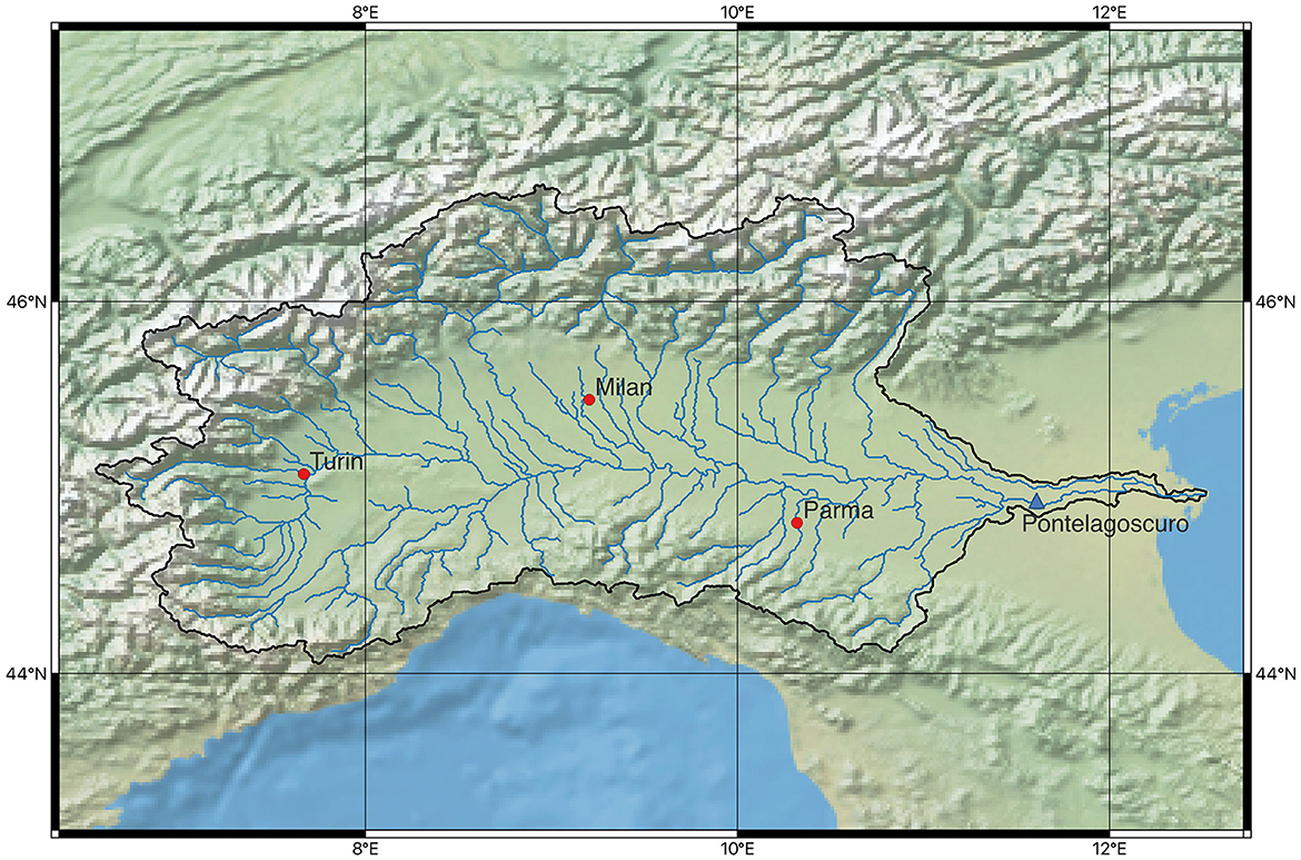
Figure 1. River Po basin area. The location of station Pontelagoscuro (PLS) is indicated by a blue triangle.
ARPA-SIM, the Hydro-Meteorological Service of the Emilia-Romagna Regional Agency for Environmental Protection, which operates the real-time River Po flood forecasting system, supplied hydrological streamflow ensemble forecasts based on Consortium for Small-Scale Modeling (COSMO) Limited Area Ensemble Prediction System (LEPS) ensemble members, which are used to force the process-based hydrological distributed model TOPKAPI (Liu et al., 2005). Streamflow routing toward gauging station PLS is performed by the Saint-Venant equation solver SOBEK (Stelling and Verwey, 2006). COSMO-LEPS is a joint development effort aimed at the improvement of short-to-medium range forecast of extreme and localized weather events in Europe. The system consists of 16 integrations of the COSMO weather model at 7-km spatial resolution that were launched on the basis of initial and boundary conditions provided by 16 representative members of the super-EPS (Molteni et al., 1996) of the European Centre for Medium-range Weather Forecasts (ECMWF).
Due to the provision of final streamflow forecasts at station PLS, it is not possible to separately quantify the uncertainties contributed by the hydrologic model from those induced by the hydraulic flood wave propagation model. However, Equation (4) indicates a formal framework for specifying and integrating different individual sources of uncertainty in the forecasting chain.
Observations and forecasts are sampled at 3-hourly time steps (Δt = 3 h), the latter consisting of an array of hourly streamflow forecasts over a 120-h horizon. The available data set covers the period from 9/11/2012 to 28/02/2015, including 842 days and 1,628 forecasting instances in total.
3.2 Processing
As a first step in data processing, we organize all streamflow forecast outputted by the 16 member EPS (m = 16) and observations for 1,628 forecasting instances such that each stream-flow forecast associated with an ensemble member compares directly against the corresponding observations. The sample of forecasts and associated observations over all selected k time steps in the 96 h forecasting horizon includes 1,628 × (m+1) values. Each sample pair is mapped into its standard Gaussian image by applying the Normal Quantile Transform (NQT). The mapping involves matching the probabilities of the empirical CDF of the original sample with those of the standard Gaussian distribution. In the standard Gaussian space, it is straightforward to establish the joint distribution (Equation 12) and the family of conditional densities (Equation 13). The latter yields k univariate predictive distributions, which are conditional on the k · m-sized multivariate distribution of predictions. The image in the real space is obtained by mapping the k univariate marginal conditional distributions back into the space of origin by inverse NQT as .
3.3 Results
Next, we present the outcome of the processing in terms of performance indicators of the time-horizon dependent MPC (MCP-THD), whereby we compare the predictive mean against (a) the raw ensemble mean (REM) and (b) the predictive mean of the time-horizon independent MCP (MCP-THI). The time-horizon independent MCP-THI (also labeled multivariate MCP; Coccia and Todini, 2011) was extensively compared by Biondi and Todini (2018) against the post-processing of forecasts using Bayesian model averaging (BMA; Raftery et al., 2005) and a univariate version of MCP. This univariate version is characterized by reduced mathematical complexity and can be convenient for applications where hydrological ensembles are provided; it considers the ensemble mean as the predictor but does not require the reordering of the ensemble members. This research demonstrates the advantage of using post-processors over direct use of raw ensembles in terms of accuracy and reliability. It also highlights, among other factors, the effects of ensemble member cross-correlation, which, unlike BMA and univariate MCP, is fully acknowledged by MCP-THI and MCP-THD.
We inter-compare REM, MCP-THI, and MCP-THD performances by executing a continuous forecast simulation over the 842-day simulation period indicated in Paragraph 3.1 and generating 1,628 forecast instances. At each of the k = 32 3-hourly time steps of the 96 h forecast horizon, we compute the Nash-Sutcliffe efficiency (NSE) and root mean square error (RMSE) performance indicators. Both indicator values, which are listed in Table 1 for increasing time horizons, clearly indicate an improvement of performance when moving from REM to MCP-THI and finally to MCP-THD. This is also made visible in Figure 2, wherein the left pane shows the decline of NSE for the three processing methods with increasing lead time, whereas the progressive forecast error growth measured in terms of RMSE is given to the right.
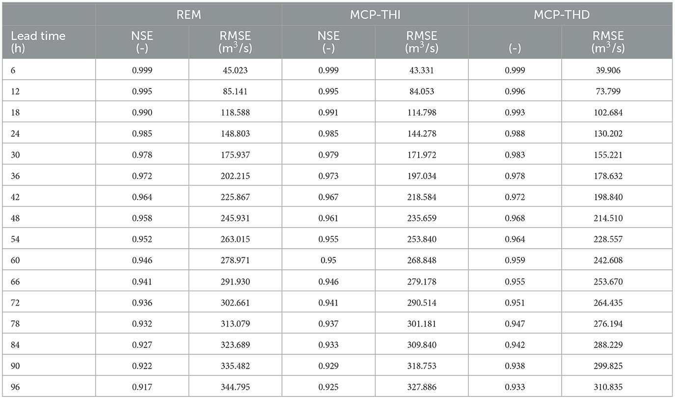
Table 1. Performance indicators for REM and the predictive means of MCP-THI and MCP-THD, 96 h lead time, Δt = 3 h, shown every 6 h: Nash-Sutcliffe efficiency (NSE) and root mean square error (RMSE); the computation is carried out for the entire database including 1,628 forecasting instances.
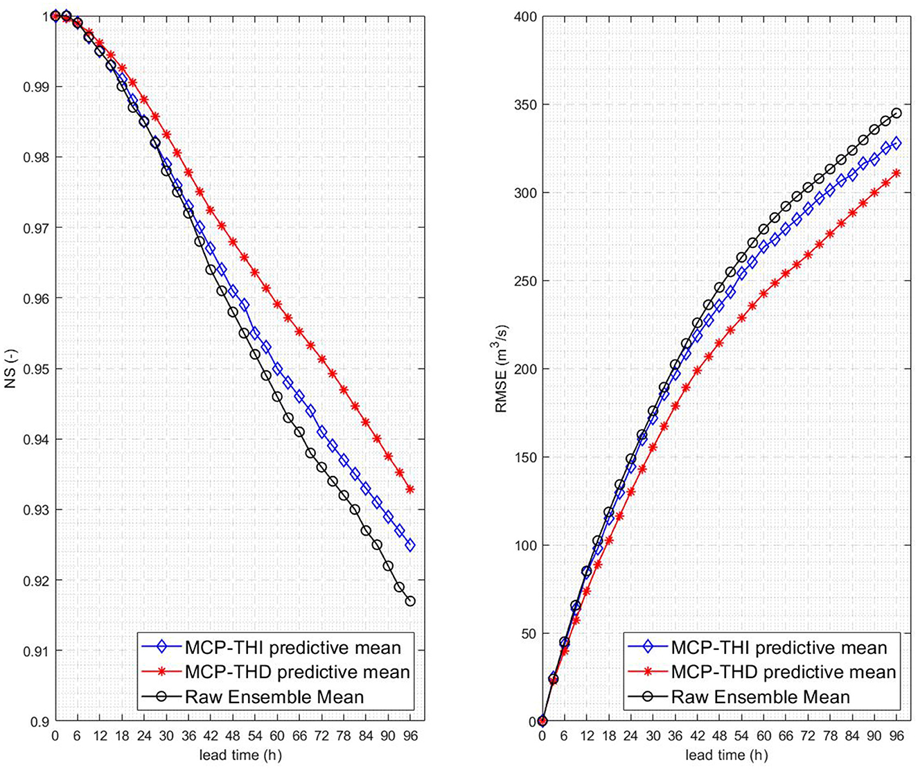
Figure 2. River Po at gauging station PLS: Nash-Sutcliffe efficiency (NSE) (left pane) and root mean square error (RMSE) (right pane) for (a) raw ensemble mean forecast, (b) the predictive mean values of MCP-THI, and (c) MCP-THD.
Figure 3 shows the evolution of the discharge forecast for four different onset times to, which approach a selected flood event on the 29/11/2012 in 3-hourly time steps. The shaded areas indicate the 90% confidence intervals tracked by the predictive distribution, and the solid black line are observations. The predictive mean, i.e., the expected value of the predictive distribution at different forecasting times, is shown by a dashed red line, whereas the 4,000 m3/s flood warning threshold is represented by the blue horizontal line.
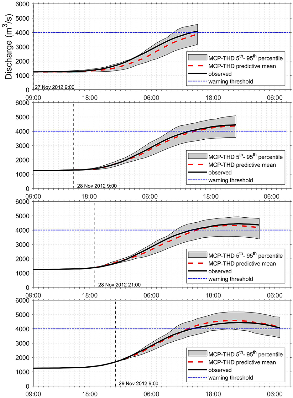
Figure 3. River Po at gauging station PLS, 29/11/2012 flood, evolution of the forecast with onset times to = 27/11/2012 21:00, 28/11/2012 09:00, 28/11/2012 21:00, and 29/11/2012 09:00. The shaded area indicate the 90% confidence interval, the solid black curve observations, and the dashed red curve the MCP-THD predictive mean. The 4,000 m3/s flood warning level is marked by the blue horizontal lines.
The very essence of the MCP-THD processor is summarized in Figure 4 for the selected flood event of Figure 3 and chosen forecast onset time to = 29/11/2012 09:00. The upper pane shows the forecast and respective 90% confidence intervals against observations. The middle pane indicates the cumulative probability density function (CDF) of threshold exceedance with changing forecasting horizon j = 1, …, k as defined by Equation (22). The lower pane shows the discrete increment ratios IR(to + jΔt) defined in Equation (24) for the same temporal increments, which equals the discrete PDF associated with the CDF. As one would expect, the probability mass is concentrated around time horizon t = 45 h, when threshold exceedance actually occurs.
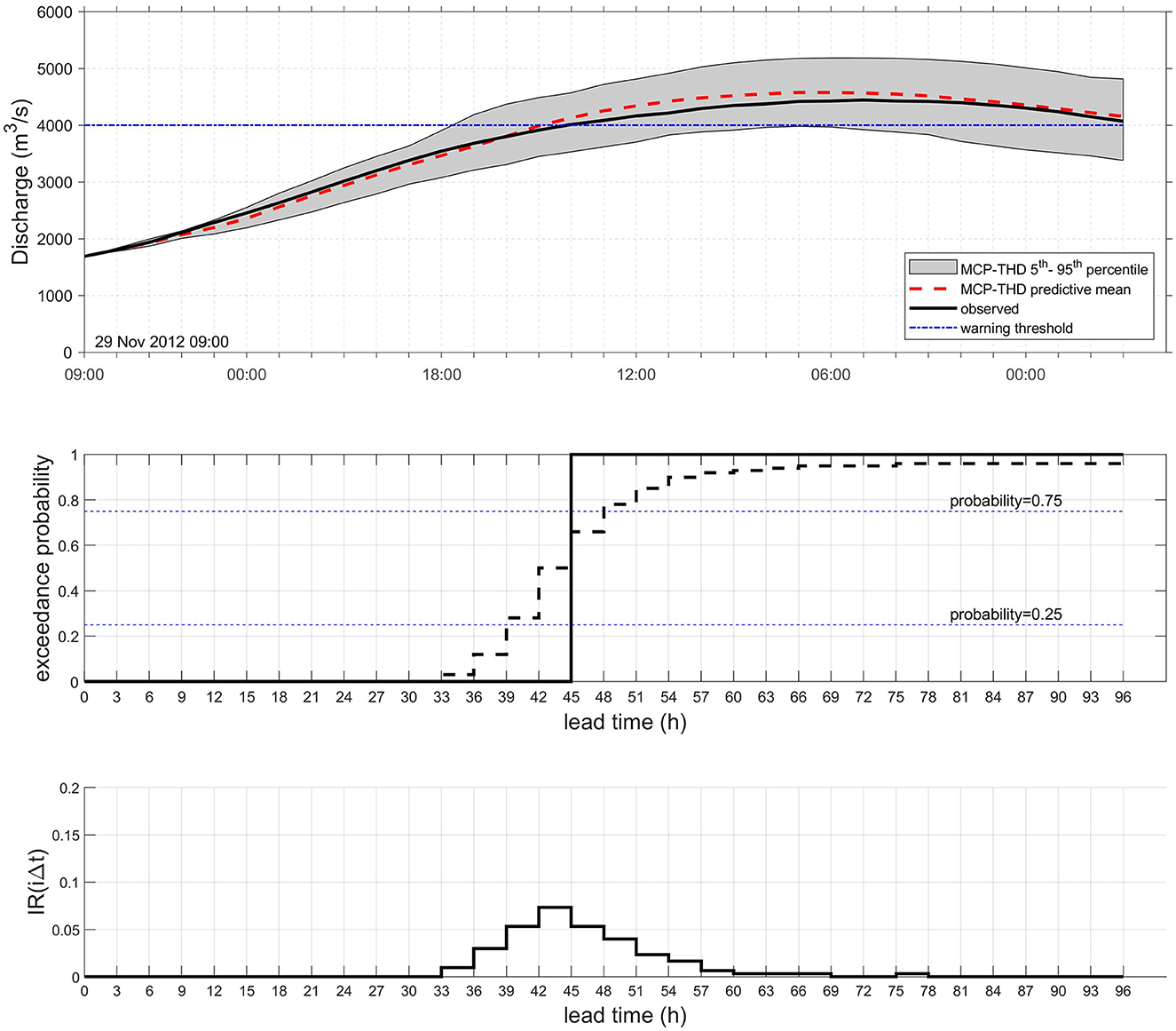
Figure 4. River Po at gauging station PLS, 29/11/2012 flood, forecast onset to= 29/11/2012 9:00. (Top) Comparison between observed (solid black line) and forecasted discharge (dashed red line) processed by MCP-THD. The shaded area indicates the 90% confidence interval; (Center) CDF of exceedance for the warning threshold of 4,000 m3/s (dashed stepwise line) and step function (solid black line) representing the probability of occurrence of the real event; (Bottom) incremental ratio IR(to + jΔt)∀j = 1, …, k of the exceedance probability, corresponding to the PDF associated with the CDF in the center pane.
Next, we examine the forecast skill of the time-horizon dependent processor against the remaining two processing methods by comparing performance indicators. These include the Threat Score (TS), Probability of Detection (POD), and False Alarm Rate (FAR). The definition of the three indicators is recalled in Appendix A. For this purpose, an event is considered each time a flow value exceeds a predefined warning threshold (e.g., 4,000 m3/s) within the forecast horizon (from 1 to 96 h following the forecast onset time to), and performance indices are consequently estimated. If we consider as flood event the one in which the peak flow exceeds the threshold value, there have been nine recorded events with peak values exceeding 4,000 m3/s during the analyzed period. Just like any model, the forecast's robustness depends on the diversity, representativeness and completeness of the training and calibration data. A greater number of events can enable the model to better understand complex relationships in the data, enhancing its ability to make more accurate and reliable predictions.
Table 2 compares the values of the performance indicators for MCP-THI and MCP-THD at different probability of threshold exceedence and three flood warning levels, respectively. In addition, here we emphasize the higher forecast skill of the time-horizon dependent approach, which is expressed in terms of larger Probability of Detection (POD), and smaller false alarm rates (FAR).

Table 2. Contingency table showing the forecasting skill for three warning levels. The results refer to different exceedance probability quantiles for MCP-THI and MCP-THD.
Figure 5 shows a forecast performance diagram. Performance diagrams were introduced by (Roebber, 2009) and provide a more concise presentation of the results. The diagram plots success ratio (SR = 1 - FAR) on the abscissa and probability of detection (POD) on the ordinate axis, along with isolines representing BIAS and Threat Score (TS), which can be expressed as functions of these measures. This type of representation facilitates a clearer visual assessment of the forecast's quality and potential biases.
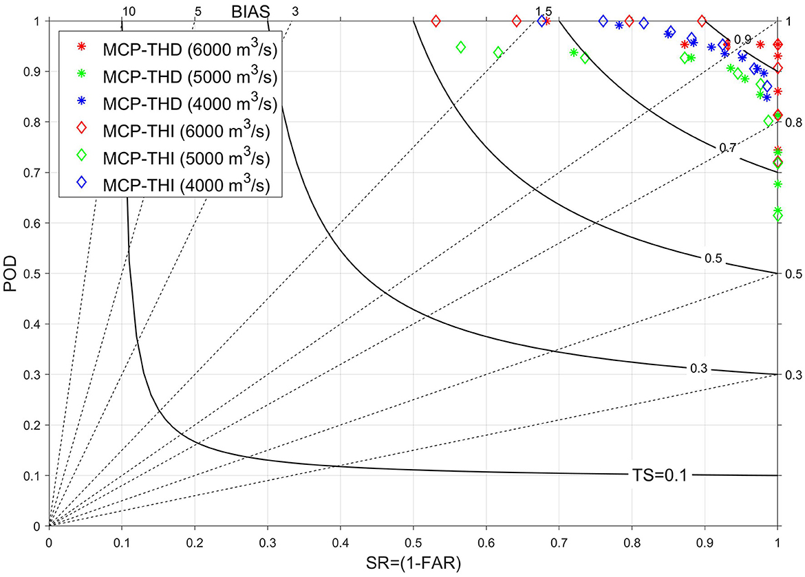
Figure 5. Performance inter-comparison diagram (Roebber, 2009) for MCP-THI and MCP-THD, different probability quantiles, and three warning thresholds. The two axes report the Probability of Detection (POD) against the success rate SR = 1-FAR. The curves connect the loci of equal Thread Scores (TS). The bisection line indicates equal probability of detection and success rate. The response bias is indicated on the top abscissa and the right ordinate axes.
4 Discussion
Biondi and Todini (2018) compared the uni- and multivariate MCP of uncertainty, with conditional mean and variance specified by Equation (16), against raw ensemble mean and model averaging with uniform and non-uniform Bayesian weighting for time-horizon independent applications. Here, we extend the time horizon-independent multivariate MCP to allow for time-horizon dependency. While this concept was adopted earlier by Barbetta et al. (2017), we revisit the main statistical concepts and provide more discussion on underlying assumptions.
The relevance of time-horizon dependent forecasting lies in the informative added value provided to a forecaster by considering the temporal correlation of the flood peak propagation process at a site. Instead of outputting just the probability of threshold exceedance given a prediction, the user is enabled to evaluate how such likelihood evolves chronologically as the event approaches. Such insights provide additional support for planning mitigating measures under operational conditions.
The most important assumption of the MCP lies in the hypothesis of modeling the dependence structure among predictors and the predictand over different time horizons as multivariate Gaussian copula, which is obtainable from standard normal images of the original marginal distributions of variates. Validating this hypothesis by measuring the distance between a multivariate Gaussian density model and the true multivariate distribution remains difficult in practice (Herr and Krzysztofowicz, 2005), mainly because of the dimensionality of the problem. However, the multivariate dependency assumption is attractive due to analytical tractability of conditional distributions. Its validity has been assessed indirectly by inter-comparison of performance indicators RMSE, MAE, and NSE for the time-horizon independent MCP against those of raw ensemble mean predictions and Bayesian model averaging (Biondi and Todini, 2018). Here, we show that the introduction of time-horizon dependency further increases processor performance as demonstrated through the indicators in Table 1 and standard skill assessment criteria in Table 2 and Figure 5. In particular, the number of false and missed alarms of MCP-THD is smaller than for MCP-THI, leading to an overall higher threat score (TS) defined by Equation (A.2). The good performance of MCP-THD is corroborated by the concentration of POD vs. 1-FAR combinations for MC-THD sited in the upper right corner of the performance diagram in Figure 5.
In the same context, we also mention that the chosen test bed system refers to a large Italian river, which is characterized by a predominantly homoscedastic (constant variance) dependency relationship among predictors and the predictand. Smaller systems, however, tend to show a behavior in which the variance changes across the variable range, and needs to be correspondingly modeled through the chosen dependency structure (Coccia and Todini, 2011). An further elaboration on this topic for the MCP-THD, however, lies outside the scope of the present research.
While probabilities of event occurrence do not depend on the probability space in which the variables are represented, an inverse transformation of the predictive Gaussian distribution into its image in the space of origin is important in an operational setting, because forecasters prefer to work with quantities and scales they are acquainted with. Although not necessary to assess the probability of occurrence of a threshold exceedance in the forecasting horizon, which can be done in the Gaussian space, where the multivariate joint distribution is known, a multivariate probability density function in the space of origin would be obtainable through Gibbs sampling (Geman and Geman, 1984). Nevertheless, such density may not be required in practice; whereas the multivariate analysis of exceedances can be performed in the Gaussian space, the marginal conditional distribution shown in Figure 4 yields operationally fully useable probabilistic forecasts of flow or stage.
The property of self-calibration for the MCP is assured in virtue of its definition through a joint density . Marginalization of the joint density with respect to predictors leads naturally to the density of historic streamflow observations, thus assuring that an MCP always falls back onto the unconditional long-term distributions of observation in the absence of informative predictors.
5 Conclusions
The study describes and promotes the use of a statistical processor designed to estimate the predictive uncertainty for an ensemble of stream flow preditors over a series of consecutive time steps across the forecasting horizon. We have demonstrated that such an extension of the original MCP to a multi-model and now time-horizon dependent version is straightforward and allows one to deal with high dimensionality problems. In the case study presented in this study, the dimension is 17 (1 series of observations plus 16 model ensemble members) times 32 (96 h forecasting horizon using 3 h time steps). In addition to the cross-correlations among multiple predictors, the processor also exploits the temporal correlations across successive forecasting time steps. Acknowledging such correlation has proven to yield multiple advantages with respect to conventional time-horizon independent processing. These can be summarized as follows:
• Time-horizon dependent forecasting does not only provide the probability of threshold exceedance for a predictand at a set future point in time but also allows tracking the flood wave across time in probabilistic terms.
• By additionally acknowledging the autocorrelation structure of the flood process, which is especially strong in highly predictable river system with slow flood motion, the forecasting error, measured in terms of RMSE and NSE, can be reduced considerably over the forecasting horizon in comparison to time-independent processing.
• Similarly, standard skill measurement indicators, including the False Alarm Rate (FAR) and the Probability of Detection (POD), show improvements over time-horizon independent processing for the selected river system.
• The advantages outlined above may diminish when smaller river systems with fast flood propagation behavior are considered. In this case, the dependency structure between predictors and the predictand becomes heteroscedastic and characterized by frequent outliers, two properties which lead do increases of the prediction error.
• To adapt the THD processor to applications with heteroscedastic behavior, the dependency needs to be modeled over different sub-ranges of the joint distributions. While this issue has been addressed preliminarly by Coccia and Todini (2011) by means of truncation, further research is needed.
Data availability statement
The raw data supporting the conclusions of this article will be made available by the authors, without undue reservation.
Author contributions
PR: Conceptualization, Writing—original draft, Writing—review & editing. DB: Conceptualization, Data curation, Investigation, Methodology, Software, Writing—original draft, Writing—review & editing. ET: Conceptualization, Writing—original draft, Writing—review & editing.
Funding
The author(s) declare financial support was received for the research, authorship, and/or publication of this article. The work has been partially funded by Deutsche Forschungsgemeinschaft grant RE 3834/10-1 awarded to PR.
Conflict of interest
The authors declare that the research was conducted in the absence of any commercial or financial relationships that could be construed as a potential conflict of interest.
Publisher's note
All claims expressed in this article are solely those of the authors and do not necessarily represent those of their affiliated organizations, or those of the publisher, the editors and the reviewers. Any product that may be evaluated in this article, or claim that may be made by its manufacturer, is not guaranteed or endorsed by the publisher.
References
Alpert, M., and Raiffa, H. (1982). “A progress report on the training of probability assessors,” in Judgment under Uncertainty: Heuristics and Biases, eds. D. Kahneman, P. Slovic, and A. Tversky (Cambridge University Press), 294–305.
Barbetta, S., Coccia, G., Moramarco, T., Brocca, L., and Todini, E. (2017). The multi temporal/multi-model approach to predictive uncertainty assessment in real-time flood forecasting. J. Hydrol. 551, 555–576. doi: 10.1016/j.jhydrol.2017.06.030
Biondi, D., and Todini, E. (2018). Comparing hydrological postprocessors including ensemble predictions into full predictive probability distribution of stream flow. Water Resour. Res. 54, 9860–9882. doi: 10.1029/2017WR022432
Brown, J. D., and Seo, D.-J. (2010). A nonparametric postprocessor for bias correction of hydrometeorological and hydrologic ensemble forecasts. J. Hydrometeorol. 11, 642–665. doi: 10.1175/2009JHM1188.1
Clark, M. P., Rupp, D. E., Woods, R. A., Zheng, X., Ibbitt, R. P., Slater, A. G., et al. (2008). Hydrological data assimilation with the ensemble Kalman filter: use of streamflow observations to update states in a distributed hydrological model. Adv. Water Resour. 31, 1309–1324. doi: 10.1016/j.advwatres.2008.06.005
Coccia, G., and Todini, E. (2011). Recent developments in predictive uncertainty assessment based on the Model Conditional Processor approach. Hydrol. Earth Syst. Sci. 15, 3253–3274. doi: 10.5194/hess-15-3253-2011
Geman, S., and Geman, D. (1984). Stochastic relaxation, Gibbs distributions and the Bayesian restoration of images. IEEE Trans. Pat. Anal. Machine Intell. 6, 721–741. doi: 10.1109/TPAMI.1984.4767596
Gneiting, T., Raftery, A. E., Westveld, A. H., and Goldman, T. (2005). Calibrated probabilistic forecasting using ensemble model output statistics and minimum CRPS estimation. Monthly Weather Rev. 133, 1098–1118. doi: 10.1175/MWR2904.1
Hamill, T. M., and Whitaker, J. S. (2006). Probabilistic quantitative precipitation forecasts based on reforecast analogs: theory and application. Mon. Wea. Rev. 134, 3209–3229. doi: 10.1175/MWR3237.1
Hemri, S., Fundel, F., and Zappa, M. (2013). Simultaneous calibration of ensemble river flow predictions over an entire range of lead times. Water Resour. Res. 49, 6744–6755. doi: 10.1002/wrcr.20542
Hemri, S., and Klein, B. (2017). Analog-based postprocessing of navigation-related hydrological ensemble forecasts. Water Resour. Res. 53, 9059–9077. doi: 10.1002/2017WR020684
Hemri, S., Lisniak, D., and Klein, B. (2015). Multivariate postprocessing techniques for probabilistic hydrological forecasting. Water Resour. Res. 51, 7436–7451. doi: 10.1002/2014WR016473
Herr, H. D., and Krzysztofowicz, R. (2005). Generic probability distribution of rainfall in space: the bivariate model. J. Hydrol. 306, 234–263. doi: 10.1016/j.jhydrol.2004.09.011
Herr, H. D., and Krzysztofowicz, R. (2010). Bayesian ensemble forecast of river stages and ensemble size requirements. J. Hydrol. 387, 151–164. doi: 10.1016/j.jhydrol.2010.02.024
Herr, H. D., and Krzysztofowicz, R. (2015). Ensemble bayesian forecasting system part I: theory and algorithms. J. Hydrol. 524, 789–802. doi: 10.1016/j.jhydrol.2014.11.072
Hersbach, R. (2000). Decomposition of the continuous ranked probability score for ensemble prediction systems. Weather Forecast. 15, 559–570. doi: 10.1175/1520-0434(2000)015<0559:DOTCRP>2.0.CO;2
Kalnay, E., Li, H., Miyoshi, T., Yang, S. C., and Ballabrera-Poy, J. (2007). 4-D-Var or ensemble Kalman filter? Tellus A 59, 758–773. doi: 10.1111/j.1600-0870.2007.00261.x
Kelly, K. S., and Krzysztofowicz, R. (2000). Precipitation uncertainty processor for probabilistic river stage forecasting. Water Resour. Res. 36, 2643–2653. doi: 10.1029/2000WR900061
Kitanidis, P. K., and Bras, R. L. (1980). Real-time forecasting with a conceptual hydrologic model: 1. Analysis of uncertainty. Water Resour. Res. 16, 1025–1033.
Koenker, R. (2005). Quantile Regression. New York, NY: Econometric Society Monographs, Cambridge University Press.
Krzysztofowicz, R. (1999). Bayesian theory of probabilistic forecasting via deterministic hydrologic model. Water Resour. Res. 35, 1757–1760.
Krzysztofowicz, R. (2001a). The case for probabilistic forecasting in hydrology. J. Hydrol. 249, 2–9. doi: 10.1016/S0022-1694(01)00420-6
Krzysztofowicz, R. (2001b). Integrator of uncertainties for probabilistic river stage forecasting: precipitation-dependent model. J. Hydrol. 249, 69–85. doi: 10.1016/S0022-1694(01)00413-9
Krzysztofowicz, R. (2014). Probabilistic flood forecast: exact and approximate predictive distributions. J. Hydrol. 517, 643–651. doi: 10.1016/j.jhydrol.2014.04.050
Krzysztofowicz, R., and Kelly, K. S. (2000). Hydrologic uncertainty processor for probabilistic river stage forecasting. Water Resour. Res. 36, 3265–3277. doi: 10.1029/2000WR900108
Liu, Z., Martina, M. L. V., and Todini, E. (2005). Flood forecasting using a fully distributed model: application of the TOPKAPI model to the Upper Xixian catchment. Hydrol. Earth Syst. Sci. 9, 347–364. doi: 10.5194/hess-9-347-2005
Maranzano, C. J., and Krzysztofowicz, R. (2004). Identification of likelihood and prior dependence structures for hydrologic uncertainty processor. J. Hydrol. 290, 1–21. doi: 10.1016/j.jhydrol.2003.11.021
Molteni, F., Buizza, R., Palmer, T. N., and Petroliagis, T. (1996). The ECMWF ensemble prediction system: methodology and validation. Quart. J. Royal Meteorol. Soc. 122, 73–119.
Pagano, T. C., Shrestha, D. L., Wang, Q. J., Robertson, D., and Hapuarachchi, P. (2013). Ensemble dressing for hydrological applications. Hydrol. Process. 27, 106–116. doi: 10.1002/hyp.9313
Pagano, T. C., Wood, A. W., Ramos, M.-H., Cloke, H. L., Pappenberger, F., Clark, M. P., et al. (2014). Challenges of operational river forecasting. J. Hydrometeorol. 15, 1692–1707. doi: 10.1175/JHM-D-13-0188.1
Raftery, A. E., Gneiting, T., Balabdaoui, F., and Polakowski, M. (2005). Using Bayesian Model Averaging to calibrate forecast ensembles. Mon. Wea. Rev. 133, 1155–1174. doi: 10.1175/MWR2906.1
Reggiani, P., and Boyko, O. (2019). A Bayesian processor of uncertainty for precipitation forecasting using multiple predictors and censoring. Mon. Wea. Rev. 147, 1–17. doi: 10.1175/MWR-D-19-0066.1
Reggiani, P., Renner, M., Weerts, A. H., and van Gelder, P. A. H. J. M. (2009). Uncertainty assessment via bayesian revision of ensemble streamflow predictions in the operational river rhine forecasting system. Water Resour. Res. 45:WR006758. doi: 10.1029/2007WR006758
Reggiani, P., and Weerts, A. H. (2008). Probabilistic quantitative precipitation forecast for flood prediction: an application. J. Hydrometeor. 3, 446–462. doi: 10.1175/2007JHM858.1
Roebber, P. J. (2009). Visualizing multiple measures of forecast quality. Wea. Forecast. 24, 601–608. doi: 10.1175/2008WAF2222159.1
Schefzik, R., Thorarinsdottir, T. L., and Gneiting, T. (2013). Uncertainty quantification in complex simulation models using Ensemble Copula Coupling. Stat. Sci. 28, 616–640. doi: 10.1214/13-STS443
Seo, D.-J., Koren, V., and Cajina, N. (2003). Real-time variational assimilation of hydrologic and hydrometeorological data into operational hydrologic forecasting. J. Hydrometeorol. 4, 627–641. doi: 10.1175/1525-7541(2003)004<0627:RVAOHA>2.0.CO;2
Stelling, G. S., and Verwey, A. (2006). Numerical Flood Simulation, Chapter 16. Hoboken, NJ: John Wiley and Sons, Ltd.
Todini, E. (2008). A model conditional processor to assess predictive uncertainty in flood forecasting. Int. J. River Basin Manag. 36, 3265–3277. doi: 10.1080/15715124.2008.9635342
Todini, E. (2012). From HUP to MCP: analogies and extended performances. J. Hydrol. 477, 32–43. doi: 10.1016/j.jhydrol.2012.10.037
Toth, Z., and Kalnay, E. (1993). Ensemble forecasting at NMC: the generation of perturbations. Bullet. Am. Meteorol. Soc. 74, 2317–2330.
Verkade, J., Brown, J., Reggiani, P., and Weerts, A. (2013). Post-processing ecmwf precipitation and temperature ensemble reforecasts for operational hydrologic forecasting at various spatial scales. J. Hydrol. 501, 73–91. doi: 10.1016/j.jhydrol.2013.07.039
Verkade, J. S., Brown, J. D., Davids, F., Reggiani, P., and Weerts, A. H. (2017). Estimating predictive hydrological uncertainty by dressing deterministic and ensemble forecasts; a comparison, with application to meuse and rhine. J. Hydrol. 555, 257–277. doi: 10.1016/j.jhydrol.2017.10.024
Vrugt, J. A., Diks, C. G. H., Gupta, H. V., Bouten, W., and Verstraten, J. M. (2005). Improved treatment of uncertainty in hydrologic modeling: combining the strengths of global optimization and data assimilation. Water Resour. Res. 41:WR003059. doi: 10.1029/2004WR003059
Wilks, D. S. (1995). Statistical Methods in the Atmospheric Sciences: An Introduction. Cambridge, MA: Academic Press.
Wood, A. W., and Schaake, J. C. (2008). Correcting errors in streamflow forecast ensemble mean and spread. JHM 9, 132–148. doi: 10.1175/2007JHM862.1
Appendix A: performance indicators
The deterministic performance indicators used in Section (3.3) for assessing the skill of the probabilistic forecasts are defined as follows.
where CA (see Table A1) is the total number of correct alarms and MA are the missed alarms. The threat score is given by the ratio:
where FA is the total number of false alarms. The False Alarm Rate is:
while the False Positive Rate is:
with CN the number of correct negative forecasts. Finally the response bias is defined as:
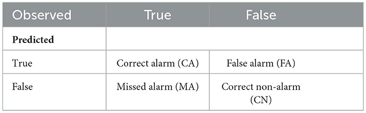
Table A1. Contingency table summarizing possible outcomes of a forecast.
All indicators are evaluated over the sample of forecasts instances.
Keywords: streamflow prediction, ensemble forecasting, post-processing, predictive uncertainty, multi-horizon, time correlation
Citation: Reggiani P, Biondi D and Todini E (2024) On time-horizons based post-processing of flow forecasts. Front. Water 6:1359750. doi: 10.3389/frwa.2024.1359750
Received: 21 December 2023; Accepted: 11 March 2024;
Published: 16 April 2024.
Edited by:
Georgia A. Papacharalampous, National Technical University of Athens, GreeceReviewed by:
Patrick Enda O'Connell, Newcastle University, United KingdomJasper Vrugt, University of California, Irvine, United States
Copyright © 2024 Reggiani, Biondi and Todini. This is an open-access article distributed under the terms of the Creative Commons Attribution License (CC BY). The use, distribution or reproduction in other forums is permitted, provided the original author(s) and the copyright owner(s) are credited and that the original publication in this journal is cited, in accordance with accepted academic practice. No use, distribution or reproduction is permitted which does not comply with these terms.
*Correspondence: Paolo Reggiani, cGFvbG8ucmVnZ2lhbmlAdW5pLXNpZWdlbi5kZQ==