Exploration of coupled surface–subsurface hydrological model responses and challenges through catchment- and hillslope-scale examples

Selected runs with a physics-based model of surface water–groundwater interactions are used to examine in detail some numerical challenges and surprising behaviors that result from discretization, nested solution schemes, coupling, boundary condition, and other factors. Regardless of the spatial scale of the model domain (field, hillslope, catchment, …), the processes that are simulated by this class of integrated models can exhibit widely varying dynamics within and across the different subsystems comprising the land surface, the unsaturated zone, and deep groundwater formations. The presence of heterogeneities, nonlinearities, and complex boundary conditions can exacerbate numerical difficulties in resolving exchange fluxes across subsystems and lead to unexpected or undesired results, including localized numerical oscillations and an upper bound on adaptive time stepping. The need for accurate tracking of surface–subsurface exchanges and for better control of aspect ratio and mesh distortion can also influence and constrain spatial and temporal discretization choices. Finally, model performance assessments can be highly sensitive to the response variables of interest. We will illustrate some of these issues via test case simulations at large (13.66 km catchment transect) and small (450 m² hillslope) spatial scales, run at time scales from 10 days to hundreds of years.

1 Introduction

Interactions between groundwater and surface water systems play a critical role in regulating important hydrological, ecological, and biogeochemical processes such as baseflow, flooding, riparian zone vegetation growth, and hyporheic zone denitrification and oxygen redistribution (Irvine et al., 2024). Recent advances in integrated groundwater–surface water models make it possible to explore in detail the interactions between the flow of water and the transfer and transport of solutes (which can include contaminants, nutrients, microorganisms, and gasses) within and across surface (overland, streams, lakes) and subsurface (aquifer and soil) domains (Paniconi and Putti, 2015). There are however persistent challenges in the development of reliable and efficient numerical models for these phenomena. When passing from subsurface-only (or surface-only) models to integrated models, customary difficulties associated with heterogeneity and variability in parameters and state variables, nonlinearities and scale effects in process dynamics, and poorly known boundary conditions (BCs) and initial system states (e.g., Sanchez-Vila et al., 2006; Vereecken et al., 2016) are compounded (more complex BCs, nested levels of iteration and time stepping, etc.) and new hurdles are introduced, namely the need to use appropriate and robust coupling schemes and representations of process interactions and feedbacks (e.g., Discacciati et al., 2002; Dawson et al., 2004; Furman, 2008).

In this study we will restrict our attention to physics-based hydrological models, i.e., models built from the governing equations for surface and subsurface water flow and solute transport, specifically the Saint-Venant or shallow water equations for surface routine, the Richards equation for variably saturated subsurface flow, and the advection–dispersion equation for mass transport. The equations are resolved via appropriate discretization techniques that allow for a detailed representation of parameter variability and boundary condition complexity. These models require reliable numerical techniques for their resolution (e.g., Miller et al., 2013; Farthing and Ogden, 2017). There is by now a quite substantial literature on the seemingly successful application of physics-based integrated surface–subsurface hydrological models (ISSHMs), including a number of model intercomparison and case studies (e.g., Sulis et al., 2010; Maxwell et al., 2014; Kollet et al., 2017; Omar et al., 2021).

While the proliferation of integrated models reflects the considerable need for these tools in a diversity of fields and applications, it is also true that hydrology-focused research studies will not typically report in detail on negative aspects of numerical performance, such as convergence difficulties, localized inaccuracies, and other anomalous behaviors. Indeed, continuing research on any already accepted model will generally focus more on adding process complexity to the model rather than on resolving legacy flaws and limitations (which workarounds – such as grid refinement – can on occasion alleviate). At the same time, studies in the numerics literature do not generally use models that are at the same level of detail (in representing heterogeneities and boundary conditions, for instance) as the current generation of ISSHMs. Thus there can be a long gap before a state-of-the-art numerical scheme demonstrated for an ideal configuration can be adapted for more complex, general-purpose models. As an example of this, the theoretical framework for a mass-conservative scheme for surface–subsurface coupling based on boundary condition switching under infiltration scenarios (Sochala et al., 2009) has not yet been extended to evaporation and mixed (storm–interstorm) scenarios. As another example, theoretically advantageous alternatives to standard Picard or Newton iteration (Paniconi et al., 1991; Kelley, 1995) for linearizing Richards’ equation, such as the L–scheme (List and Radu, 2016; Stokke et al., 2023), exist but have not yet been fully vetted for ISSHMs, where factors such as highly varied BC types and strong subsurface heterogeneity can introduce implementation and performance challenges.

Given the complexities of physics-based ISSHMs and their continuing evolution, it is important to highlight some of the undesirable or unexpected numerical results that can occur when running these models, as this may in some measure help guide the development of new or improved equation solvers and discretization schemes for strongly coupled and highly nonlinear systems, and ultimately contribute to future improvements to ISSHMs. Moreover, the coupling itself, manifested across an interface between disparate flow domains and through intricate boundary conditions or exchange terms, can raise new issues for both established and emerging numerical schemes for solving the flow equations, and test simulations with an ISSHM can help to identify these.

Within this context, we seek to illustrate in this study, via example simulations, some of the numerical challenges and surprising behaviors that arise in the use of a physically based, integrated model of surface water and groundwater flow. The approach here is empirical rather than systematic, with the only strictly organizational element being in the selection of the two test cases: one at a quite large spatial scale (a 13.66 km catchment transect) run at very long time scales (hundreds of years) and the other at a small spatial scale (a 450 m² hillslope) run at a time scale of days. We will use the CATHY (“catchment hydrology”) ISSHM (Camporese et al., 2010; Weill et al., 2011) for all the simulations. This is a widely applied and fully tested model that uses numerical schemes that are standard for this class of hydrological model. In the hillslope example we will examine how activating the coupling scheme and surface routing module in CATHY impacts rainfall–runoff partitioning, including a contribution to ponding that cannot occur when surface–subsurface interactions are not fully resolved. In the transect example we will explore different land surface boundary condition settings, temporal and spatial discretization challenges, and the meaning of a steady state when flow conditions are strongly nonlinear.

2 Methods

2.1 CATHY model

CATHY is a coupled surface water–groundwater model with subsurface flow represented by the 3D Richards equation, solved by Galerkin finite elements, and surface flow represented by a path-based (quasi-2D) Saint-Venant equation, solved by a Muskingum-Cunge finite difference scheme. Analogous numerical schemes are used for the 3D advection–dispersion and quasi-2D advection–diffusion solute transport equations. A preprocessing analysis of the digital elevation model (DEM) of the topographic data identifies the drainage network and distinguishes overland (hillslope) and channel (stream) flow cells, which can then be parameterized separately (Orlandini et al., 2003; Orlandini and Moretti, 2009). This novel path-based representation of surface routing allows for a unified treatment of overland and channel flow and transport (same governing equation, different parameterizations).

Coupling between the subsurface and surface flow modules is through a boundary condition switching approach (Putti and Paniconi, 2004), whereby Neumann (specified flux) or Dirichlet (specified head) conditions are dynamically imposed according to the saturation status of a surface node (ponded, saturated, unsaturated, and air dry). At each time step, once the subsurface equation is solved, a water balance is calculated at each surface node between the atmospheric water supply (precipitation) or demand (potential evapotranspiration), the capacity of the soil to infiltrate or exfiltrate this water, and any ponded water already present at the surface. Any excess of water accumulated at the surface (ponding) becomes available for routing by the surface solver if it exceeds a threshold parameter (minimum water depth before surface routing can occur). Through this procedure, CATHY automatically tracks both infiltration excess (Hortonian) and saturation excess (Dunnian) overland flow generation mechanisms. This boundary condition-based coupling algorithm is one of three common approaches used in ISSHMs (e.g., Haque et al., 2021), and it has been theoretically shown to ensure pressure and flux continuity at the land surface interface (Sochala et al., 2009), at least under the infiltration case that was analyzed. Note that transpiration is not included in the version of CATHY used in this study, thus potential evapotranspiration data input to the model is resolved (converted into an exfiltration flux from the soil) according to a BC switching scheme for actual evaporation that is analogous to the scheme used for rainfall–runoff partitioning.

2.2 Test cases

The hillslope-scale test case (Figure 1) is from the Biosphere 2 Landscape Evolution Observatory (LEO). See Niu et al. (2014a) and Scudeler et al. (2016a) for a description of LEO and of the CATHY experiments on this hillslope. For the runs reported in this study we used a uniform discretization at the surface (Δx = Δy = 1 m; 30 m × 15 m total) and 20 layers of equal thickness vertically (Δz = 7.5 cm; 1.5 m total), for a grid of 10,416 nodes. The average terrain slope is 17.6% (10°), with a maximum slope of 30.6% (17°) around the outlet or convergence zone.

Figure 1

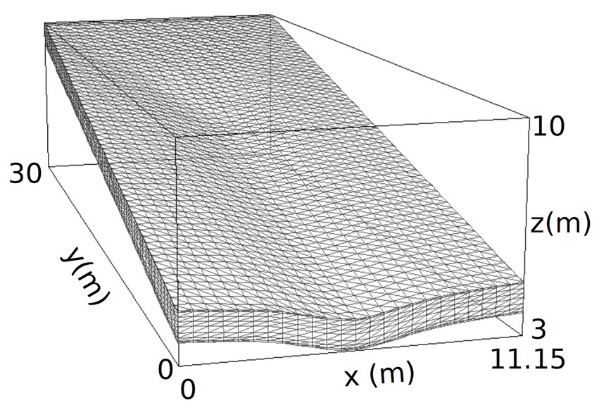
Figure 1. The LEO hillslope test case showing the uniform mesh discretization.

The transect test case (Figure 2) is from the 425 km² Tony Creek subcatchment near the town of Fox Creek in west-central Alberta, Canada. See Meneses-Vega et al. (under review)¹ for a detailed presentation of the 700 km² Fox Creek study area and of the CATHY applications in both two-dimensional (2D transect) and fully 3D configurations. For the runs reported in this study we used a uniform discretization along the transect (Δx = 20 m; 13.66 km total) and 15 layers of varying thickness vertically (from 15 cm to 60 m; 300 m total), for a grid of 32,832 nodes (this includes a 3-node discretization in the no-flow transverse direction since CATHY is a 3D model). A finer layering was used near the surface and toward the base of the domain, in order to more accurately resolve the atmospheric forcing and free drainage boundary conditions. The average terrain slope is 1.7% (1.0°) on the transect segment to the right of the creek (valley bottom) and 1.6% (0.9°) to the left, with a maximum slope of 6.8% (3.9°) along the right streambank.

Figure 2

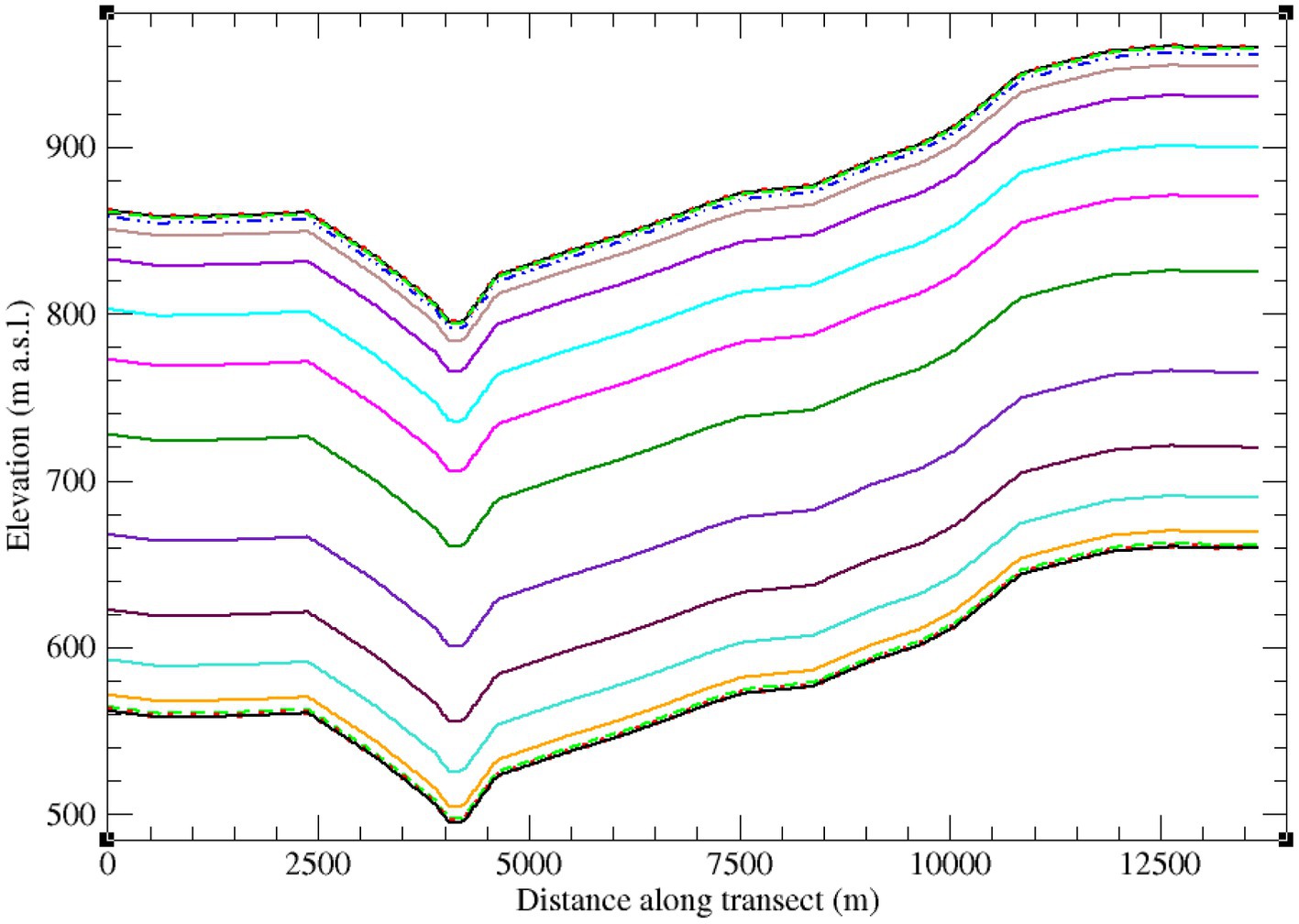
Figure 2. The Tony Creek transect test case showing the vertical mesh discretization.

The soil and aquifer parameter values for these two test cases are summarized in Table 1.

Table 1

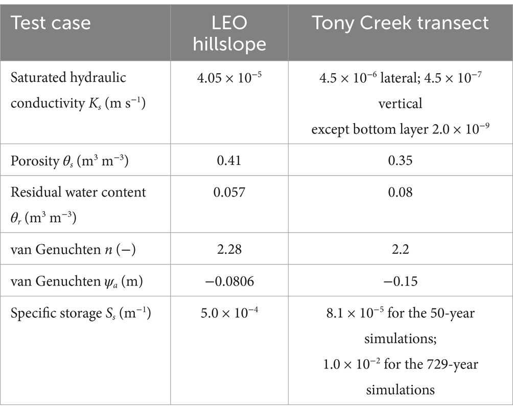
Table 1. Parameter values for the two test cases.

3 Results

3.1 LEO hillslope example

For the CATHY simulations on LEO, the hillslope was initially completely unsaturated, with a pressure head distribution obtained from a long-term drainage experiment. Drainage occurs across a Dirichlet (zero pressure head) boundary condition imposed at the 16 nodes along the bottom of the downslope face of the hillslope, with the highest outflows in the middle of this face, in correspondence with the hillslope’s planform. The soil for this experiment was considered homogeneous and isotropic (these assumptions were relaxed in subsequent LEO trials with CATHY, reported in Niu et al., 2014a; Pasetto et al., 2015; Scudeler et al., 2016a), with saturated hydraulic conductivity K_s = 4.05 × 10⁻⁵ m/s, porosity θ_s = 0.41, specific storage S_s = 5 × 10⁻⁴ m⁻¹, and van Genuchten (1980) soil water retention curve parameter values of: fitting exponent n = 2.28, residual moisture content θ_r = 0.057, and air entry pressure head ψ_a = −0.0806 m (see Table 1). The experiment was of a 10-day (8.64 × 10⁵ s) duration and comprised four precipitation events generated by the rainfall generator at LEO: 180 mm/h (5.0 × 10⁻⁵ m/s) for a duration of 20 min, 0.9 mm/h (2.5 × 10⁻⁷ m/s) for 2 d, 9 mm/h (2.5 × 10⁻⁶ m/s) for 12 h, and 90 mm/h (2.5 × 10⁻⁵ m/s) for 3 h (Figure 3). Since K_s is smaller than the rainfall rate of the first event, infiltration excess runoff is generated during this event. For the middle two (low rainfall) events, no surface runoff is produced. For the last event, notwithstanding the initially quite dry soil conditions and the presence of a Dirichlet BC at the base of the hillslope, Dunne saturation excess runoff is produced over a portion of the hillslope. We will examine more closely the surface saturation response of the hillslope in the next section. Here we will look instead at the fluxes that are generated.

Figure 3

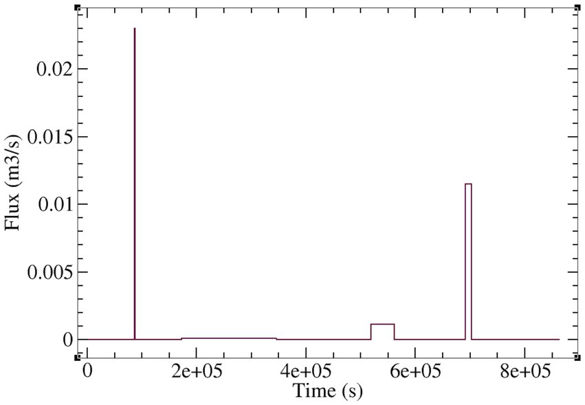
Figure 3. Atmospheric forcing for the 10-day (8.64 × 10⁵ s) LEO experiment showing the four rain events.

3.1.1 Flux partitioning

The impact of surface–subsurface interactions can be seen in Figure 4 were fluxes imposed (atmospheric BC) and generated by the model (actual, overland, and return flow) are plotted for the first (top graph) and last (bottom graph) rain events for CATHY simulations with and without coupling (in no-coupling mode, only the subsurface module is run). In the first (Horton runoff-generating) event, when the rainfall period ends the actual flux (infiltration rate) falls to zero in the subsurface-only run, whereas in the coupled run infiltration persists because there is some water that has accumulated at the surface from the runoff generation and routing processes, seen as the green overland flow curve (negative after the rain event because it is subtracted from the rainfall rate). Even during the rainfall period, the actual flux is slightly higher in the coupled case because any ponded water amount is “added” to the rainfall rate, creating a stronger head gradient for infiltration after the “time to ponding” is reached. There is no return flow (exfiltration across a ponded or saturated surface) for the first event because below the land surface the soil profile is still unsaturated.

Figure 4

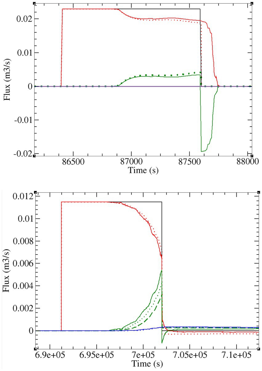
Figure 4. Atmospheric input (rainfall) flux (black), actual flux across the land surface (red), overland flow rate (green), and return flow rate (blue) for CATHY in coupled (surface–subsurface flow and transport) mode (solid lines) and uncoupled (subsurface flow and transport only) mode (dotted lines) for the first (top graph) and last (bottom graph) rain events of the LEO hillslope test case. The dashed green line is for a subsurface flow only (i.e., no transport) run.

For the last (Dunne runoff-generating) event, we again see post-event persistence of infiltration for the coupled run, of a smaller magnitude and duration here because the rainfall rate is much lower than the first event. During the rainfall period, the actual flux is now slightly lower in the coupled case than in the subsurface-only case. This is because there is now return flow occurring in the fully saturated portion of the hillslope (downslope around the convergence zone), making the net (downward) infiltration lower. Later in the simulation (and not shown here), some of this exfiltration eventually reinfiltrates into the soil. The dashed green curve in the plot for the last rain event is from a CATHY run with no coupling and no solute transport (so subsurface flow only). We observe that overland flow is higher when transport is active, indicating an additional dispersive or mixing layer impact on surface–subsurface interactions (Gatel et al., 2020; Gatto et al., 2021) that is highly complex and possibly conditioned by how boundary conditions are treated. This effect requires further study, as indeed do many aspects of solute transport handling in ISSHMs, which has received much less attention in the literature compared to flow modeling. Solute transport will not be considered in the Tony Creek example.

3.1.2 Surface saturation response

For the same two events for which we examined flux partitioning across the land surface interface in Figure 4, we now look at the saturation response of this boundary. The top graph in Figure 5 shows the fraction of the hillslope surface that is saturated during the first and most intense of the four rain events. Since the rainfall rate exceeds the K_s of the surface, and since this event occurs early in the 10-day simulation period when the soil is still quite dry throughout the hillslope, only Horton runoff occurs here. Moreover, since K_s is homogeneous, when saturation does occur, it occurs over the entire hillslope, and thus the saturation fraction reaches 1. The time to ponding is quite rapid (about 500 s after the start of the rain event), and is roughly but not exactly equal over the entire hillslope, due to a nonuniform distribution of soil moisture at the start of the event. As in the preceding section, the inclusion or not of solute transport appears to influence the flow responses produced by the model. Also noteworthy is the difference between the coupled and uncoupled model at the end of the rain event. In the coupled case, even though the atmospheric flux is now zero, Horton saturation persists for a short period after the rain has ceased (and the degree of saturation gradually rather than abruptly drops to zero) because of the spatial distribution of ponded water that provides a supplemental input flux. This ponding-assisted Horton saturation is an interesting counterpoint to Horton-assisted upstream expansion of a catchment’s Dunne saturated areas reported in Zanetti et al. (2024). These phenomena are a direct result of using an integrated model, and they should be explored in more detail.

Figure 5

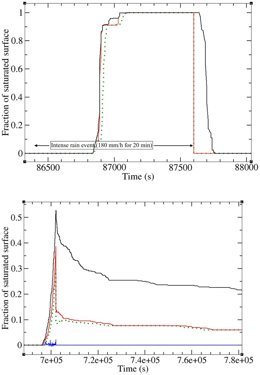
Figure 5. Coupled (black), subsurface only (red), and subsurface flow only (i.e., no transport) (green) saturation responses for the first (top) and last (bottom) rain events of the LEO hillslope test case. The blue curve in the bottom graph is the Horton contribution to surface saturation that is produced in the coupled case.

For the last rain event (bottom graph), Dunne runoff occurs for all model runs (and notwithstanding the Dirichlet BC at the base of the hillslope, as mentioned previously), and it is clearly spatially nonuniform due to topography, slope, and planform effects. The influence of surface–subsurface interactions is very marked here, with a higher peak in surface saturation (over 50% for the coupled run compared to under 40% for the uncoupled runs) and a more persistent tail in its spatial distribution as the runoff event recedes. The blue curve in this graph at near-zero shows the Horton saturation fraction for the coupled run. There is no Horton saturation for the uncoupled runs, as expected since the rainfall rate is lower than K_s for this event. The surprising occurrence of a small amount of Horton saturation in the coupled case is again due to the presence of ponded water.

3.2 Tony Creek transect example

For the CATHY simulations on Tony Creek, the transect was initially in vertically hydrostatic equilibrium with the water table 2 m below the surface throughout the domain. Different combinations of boundary condition settings and specific storage values were used, as described in the following sections. The soil and aquifer for this experiment were considered homogeneous (this assumption was relaxed in subsequent Tony Creek trials with CATHY, reported in see footnote 1) but not isotropic, with lateral K_s = 4.5 × 10⁻⁶ m/s, vertical K_s = 4.5 × 10⁻⁷ m/s (except for the bottom layer), porosity θ_s = 0.35, and van Genuchten soil water retention curve parameter values of: fitting exponent n = 2.2, residual moisture content θ_r = 0.08, and air entry pressure head ψ_a = −0.15 m (see Table 1). The atmospheric forcing consisted of a constant rainfall rate of 70 mm/y (= 2.22 × 10⁻⁹ m/s = 6.065 × 10⁻⁵ m³/s), and free drainage was imposed at the bottom of the domain, at a rate of 2 × 10⁻⁹ m/s (= 5.464 × 10⁻⁵ m³/s), or just slightly lower than the rainfall rate. To impose this rate in CATHY, the vertical saturated hydraulic conductivity of the bottom layer was set to the desired free drainage value.

3.2.1 50-year simulations with low specific storage

Figure 6 presents the results from several 50-year simulations using a specific storage (S_s) value of 8.1 × 10⁻⁵ m⁻¹. The response variables shown, together with the imposed rainfall and free drainage fluxes, are the actual flux across the land surface, the return flow rate, and the overland flow rate. Five simulations were performed: Run 1, with no coupling (i.e., subsurface flow only) and with no boundary conditions imposed besides the atmospheric forcing; Run 2, with no coupling and with Dirichlet BC imposed at the stream node (valley bottom in Figure 2); Run 3, with no coupling and with seepage face BCs imposed along 4 nodes on either side of the valley and including the stream node; Run 4, no coupling and with seepage face BCs imposed along 25 nodes on either side of the valley and including the stream node; and Run 5, coupled with no BCs on the surface but with a designated outlet cell for the surface routing module. In addition to these response variables, Figure 6 also shows the fluxes across the seepage face boundary for Runs 3 and 4 and the outlet hydrograph for Run 5.

Figure 6

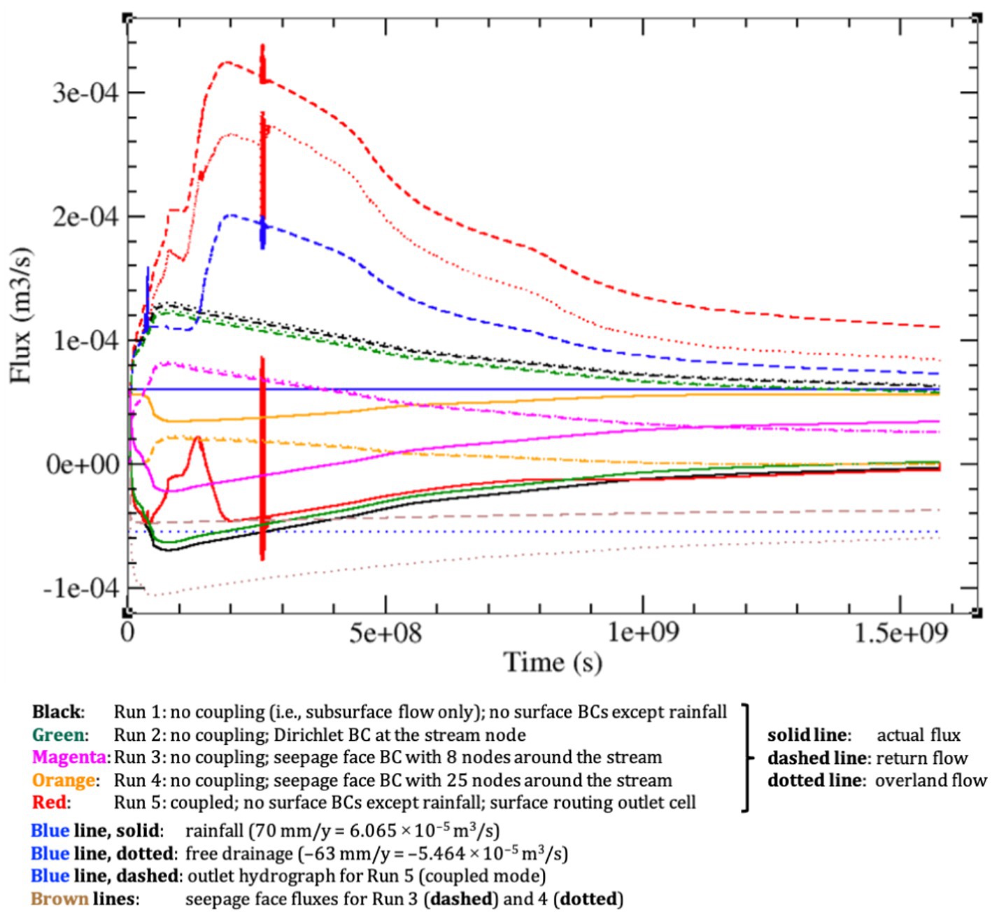
Figure 6. Results for five 50-year (1.5768 × 10⁹ s) simulations of the Tony Creek transect. Imposed incoming (rainfall = 70 mm/y = 2.22 × 10⁻⁹ m/s = 6.065 × 10⁻⁵ m³/s, solid blue line) and outgoing (free drainage = −63 mm/y = −2 × 10⁻⁹ m/s = −5.464 × 10⁻⁵ m³/s, dotted blue line) fluxes are shown, together with the actual flux across the land surface, the return flow rate, and the overland flow rate (respectively solid, dashed, and dotted curves) for: Run 1 (no coupling, i.e., subsurface flow only, and no BCs imposed on the surface besides the rainfall) in black; Run 2 (no coupling and Dirichlet BC imposed at the stream node) in green; Run 3 (no coupling and seepage face BCs imposed along 4 nodes on either side of the valley and including the stream node) in magenta; Run 4 (no coupling and seepage face BCs imposed along 25 nodes on either side of the valley and including the stream node) in orange; and Run 5 (coupled and no BCs on the surface but with a designated outlet cell for the surface routing module) in red. In addition, the brown curves are the fluxes across the seepage face boundary for Runs 3 (dashed) and 4 (dotted), and the dashed blue curve is the outlet hydrograph for Run 5.

In Figure 7 the land surface saturation responses for the coupled simulation (Run 5) and three of the uncoupled cases (Runs 1, 2, and 3) are shown. The responses for these latter 3 runs are visually identical. All of the responses in this graph are from the saturation excess runoff mechanism, except for a small occurrence of infiltration excess runoff for Run 2, discussed later in this section.

Figure 7

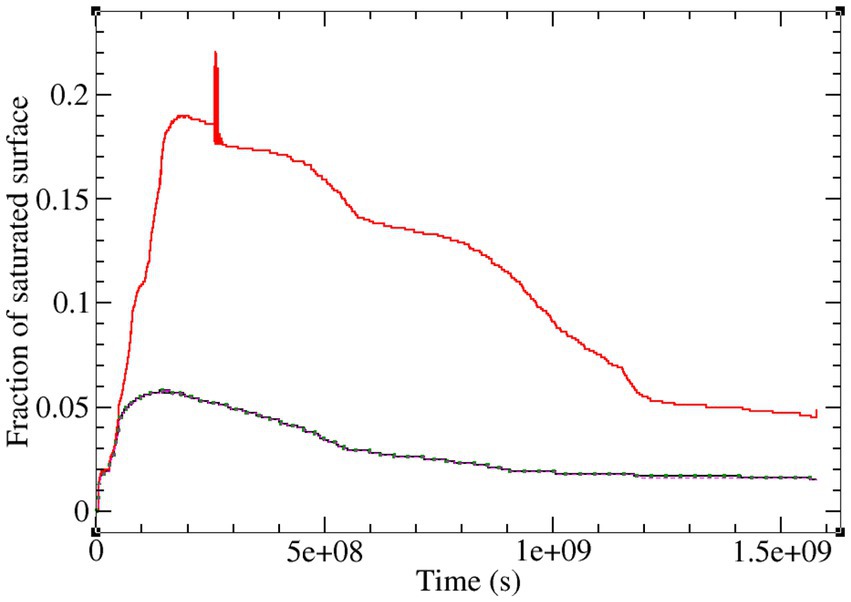
Figure 7. Land surface saturation response for the coupled simulation (Run 5) in red and for three of the no coupling runs: no BCs, Run 1 (solid black curve); Dirichlet BC at the stream node, Run 2 (dotted green curve); and seepage face BC along 8 nodes, Run 3 (dashed magenta curve). The curves for Runs 1, 2, and 3 are visually identical.

Figure 8 shows the ponding dynamics along a 200 m section across the stream channel valley, and centered at the stream node, for the coupled simulation (Run 5). In the time snapshots we see that noticeable ponding first occurs between the first and sixth month of simulation (at time 0 the water table is uniformly 2 m below the surface, and the rainfall rate is more than two orders of magnitude smaller than the vertical K_s), that the ponding levels increase until 10 years, and that they recede thereafter. It is also evident that the recession is very slow, and is perhaps reaching a steady state by the end of the simulation. Note that the spatial resolution for the output extracted for this graph is rather coarse, as only three nodes spaced 100 m apart were sampled out of the 11 nodes spaced 20 m apart.

Figure 8

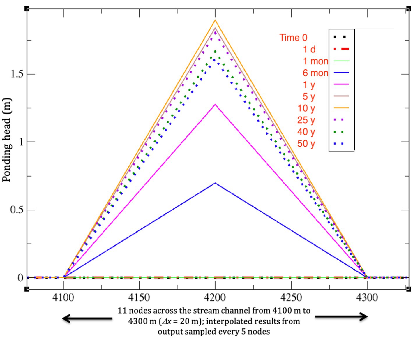
Figure 8. Ponding dynamics along a 200 m section across the stream channel valley, and centered at the stream node, for the coupled simulation (Run 5).

Several points emerge from the five 50-year Tony Creek transect simulations shown in Figures 6–8 (some of these remarks apply also to the 729-year simulations of the next section). In uncoupled (subsurface only) mode (Runs 1–4), the model is able to reproduce “expected” (for an uncoupled run) dynamics at the land surface even without imposing any of the standard boundary conditions that are typically applied in simulations of this sort. Indeed, the generated fluxes at the land surface (infiltration, surface runoff, return flow, etc.) are generally very similar between the no BC, Dirichlet BC, and seepage face cases. This underscores the role of topography in driving the hydrologic responses for transects (and watersheds) such as the one analyzed here (climate and soil parameters are uniform – except for vertical K_s at the bottom of the domain – and thus do not exert significant control over the spatiotemporal dynamics observed).

In coupled mode (Run 5) all the responses are very different from the uncoupled responses, underscoring the importance of including a proper representation of surface–subsurface interactions when these phenomena are of interest. This means not just capturing instantaneous interactions (e.g., rainfall exceeding infiltration capacity at a given point on the land surface), but also allowing for continuous interactions (e.g., overland flow generated at one point and reinfiltrating further downslope). This is apparent both in the land surface fluxes shown in Figure 6 and in the land surface saturation response shown in Figure 7. It is clear from Figure 7 that accounting for surface–subsurface interactions leads to a much greater fraction of the land surface actively contributing to the overall dynamics.

For the coupled run, we observe in Figure 6 a double hump in the rising limb of the outlet response (and also to some degree in the other response variables for this run). This response likely reflects different characteristic time scales of the shorter and steeper transect to the left of the stream and the longer right side. We also see for this run that the return and overland flow hydrographs are significantly higher than the outlet hydrograph. This is another manifestation of continuous or recycled interactions (as runoff is routed downslope), and of the fact that not all surface runoff reaches the outlet.

In the coupled run we also observe spurious numerical oscillations that may be indicative of time stepping or coupling algorithm constraints in the discretization schemes (Dagès et al., 2012; Fiorentini et al., 2015). This is a complex issue as there are numerous time stepping and iteration nestings in the numerical solution procedure (linearization of Richards’ equation; different characteristic time scales and time step constraints between the saturated zone, the vadose zone, overland flow, and channel flow; BCs that can switch from iteration to iteration and from time step to time step). Since the oscillations were only observed for the coupled run, it is not thought to be an issue connected to resolution of the subsurface flow system. It also does not appear to be an issue with the substepping scheme of the surface flow solver. This scheme is based on a Courant number criterion wherein the number of surface solver time steps is calculated at each subsurface solver time step (Camporese et al., 2010). Many tests for the Tony Creek transect were run using both tighter and looser Courant targets (the target is normally set to a value of 1.0). Increasing the target value allows for larger surface routing time step sizes, while decreasing it means that more substeps are taken within each subsurface time step. Neither increasing nor decreasing the Courant target had an impact on the oscillations. Dismissing the surface or subsurface solvers, taken separately, as possible causes, the explanation for the observed oscillations is thought to lie in the coupling scheme. For instance, the boundary condition switching algorithm may need to be improved to allow a smoother buildup of ponding heads when Dirichlet BCs are activated, or the convergence criterion on the subsurface solver needs to be based not only on convergence of the nodal pressure head solution (as is currently the case), but also on convergence of the BC switching procedure (to Dirichlet or Neumann type) at any given surface node. The oscillations are concerning and these conjectures need to be further investigated, but it should also be noted that this behavior is localized and does not persist, intensify, or otherwise affect the overall solution. In other words, this erratic behavior of an episodic nature does not point to numerical instabilities in the schemes used to resolve the surface and subsurface model equations and their coupling.

For the uncoupled runs, it is clear that by allocating a greater portion of the land surface to be a potential seepage face, the outflow across this BC increases while the overland and return flow rates are diminished, as is the amplitude and variation of the actual flux across the surface. The 4-node (Run 3) and 25-node (Run 4) seepage face BC configurations were chosen to approximately mimic, respectively, the Dirichlet BC case and the maximum extent of the variably saturated area that develops around the stream. A more detailed discussion of seepage face BCs in the context of coupled and uncoupled hydrological modeling can be found in Scudeler et al. (2017). For the Dirichlet BC simulation (Run 2), not visible in the hydrographs in Figure 6 is that initially, and until the water table reaches the surface at the stream location, this BC acts as a source of water, meaning that an important mass balance error is being committed since this water does not actually exist. This even causes a small amount of Horton runoff (to a maximum land surface saturation fraction of 0.1% in the first 20.4 d of the simulation). Therefore, care is needed when applying Dirichlet BCs at the land surface, as they may not serve their intended purpose (a drain or sink of water, for instance) during the entire course of a simulation.

It is worth noting that ponding (and thus also land surface saturation) develops at other points along the transect besides along the stream channel, in particular where there are small topographic dips (see Figure 2). However, the ponding levels observed are very small (<1 mm, compared to a peak of almost 2 m at the stream, as shown in Figure 8), and they drop to zero well before the end of the 50-year simulation.

3.2.2 729-year simulations with high specific storage

Very many simulations of the Tony Creek transect were run before arriving at the 50-year scenario described in the previous section. Three recurring, and to some degree surprising, outcomes in these trials were (a) that, although driven by steady and uniform atmospheric forcing and bottom leakage, it was not altogether clear that the flow system was approaching a steady state; (b) that any emergence of a steady state, and the eventual rate at which such a state was being approached, appeared to depend on the response variable being examined; and (c) that there was evidently a very strict and persistent upper limit to the time step size that could be used during the simulation. With regard to point (c) it was moreover observed that altering the value of the specific storage coefficient had a direct impact on the apparent maximum time step size that could be used during a simulation. Since in the governing subsurface flow equation for a saturated system, in both its continuous and discretized forms, S_s also has a direct impact on the system’s evolution to steady state (larger S_s implies slower dynamics), it was decided to further pursue issues such as the three enumerated above by running a longer simulation with a larger value of S_s. Note that any hypothesized direct link between a system’s storage coefficient, its rate of progression toward a steady state, and eventual upper constraints on time step size in a numerical discretization of the system’s governing equation may be quite tenuous for a nonlinear system (e.g., unsaturated or variably saturated zone), as indeed we are dealing with here, as opposed to a fully saturated system (saturated domain).

Following the above reasoning, in this section we present the results from simulating the Tony Creek transect for a 729-year period and with a specific storage value of S_s = 0.01 m⁻¹. The time series of the actual flux, return flow, overland flow, and groundwater recharge response variables are shown in Figure 9. The results are plotted on a linear time axis (top graph) as well as on a logarithmic time axis (bottom graph). The latter gives a better picture of the early-time behavior of the response variables, including the onset of rainfall–runoff partitioning and overland flow. Moreover, while in the top graph it might appear that the response variables are all asymptotically approaching a steady state value, in the bottom graph it is not at all evident, except for the groundwater recharge, that a steady state is imminent.

Figure 9

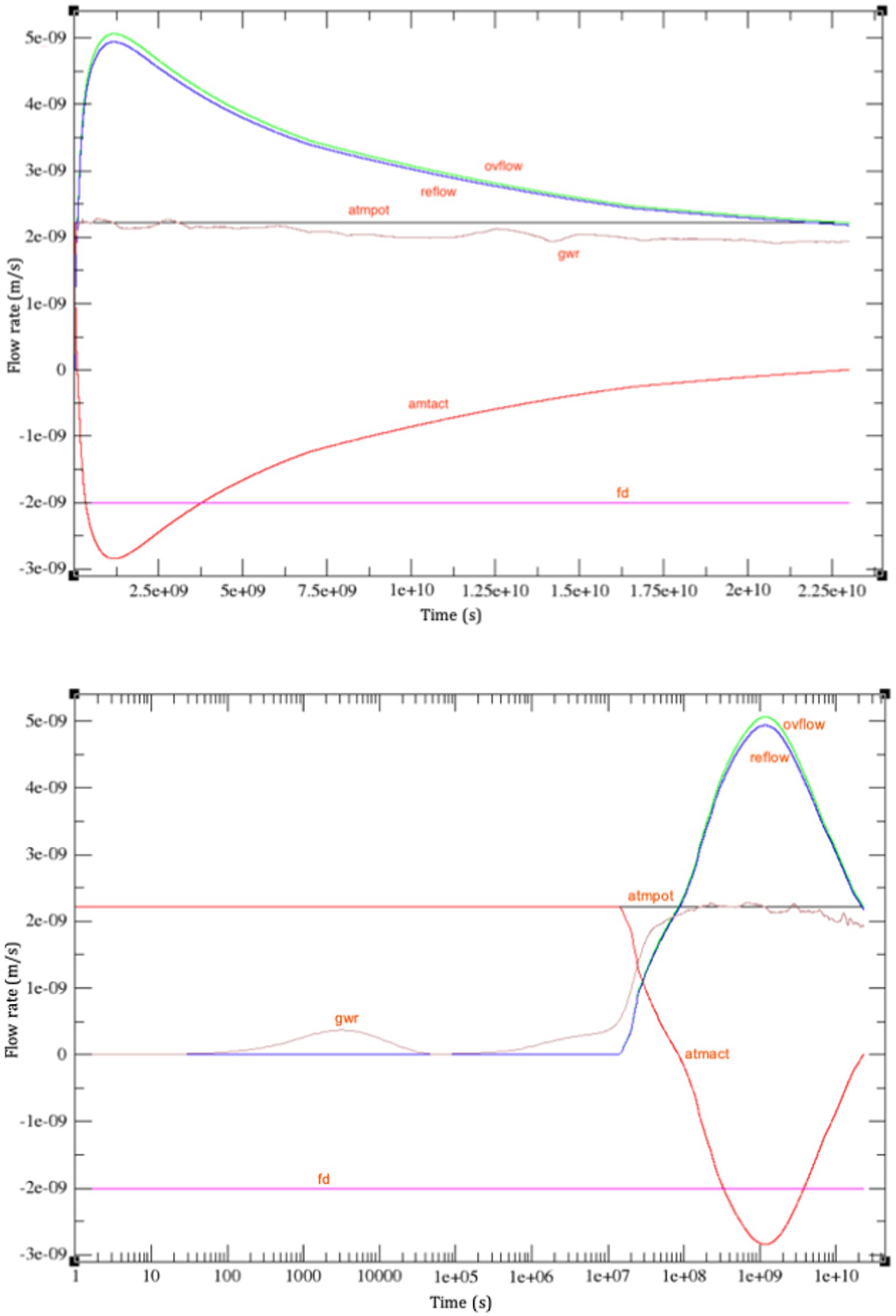
Figure 9. Results for a 729-year (2.3 × 10¹⁰ s) simulation of the Tony Creek transect. The run is driven by a constant rainfall (black line; labeled “atmpot”) of 70 mm/y (2.22 × 10⁻⁹ m/s) and a free drainage flux of −2 × 10⁻⁹ m/s (magenta; “fd”). The response variables shown are the actual flux across the land surface (red; “atmact”), the return flow rate (blue; “reflow”), the overland flow rate (turquoise; “ovflow”), and the groundwater recharge flux (brown; “gwr”). The results are plotted on a linear time axis (top graph), as well as on a logarithmic time axis (bottom graph).

Another response variable, the water table level, is shown in Figure 10 and suggests as well that a steady state is still elusive after 729 years. It seems from these results that the water table will keep dropping at the highest elevations, and perhaps even in the valley around the stream node, eventually leading to the creek becoming a losing stream (i.e., the valley becoming a point of groundwater recharge) rather than a gaining stream. Much longer simulations would be needed to establish this.

Figure 10

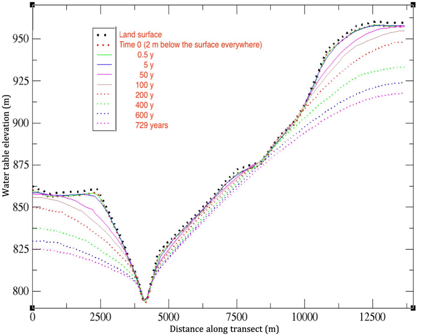
Figure 10. Water table dynamics for the 729-year simulation.

Moreover, as the water table drops and the depth of the unsaturated zone increases in the upslope regions of the transect, the amount of return flow decreases (less groundwater is contributing to it), and as a result the actual flux across the land surface (see Figure 9) gradually decreases in magnitude. In fact it appears to approach zero (from negative values) and does not return to positive values, meaning that in this later stage of the simulation, practically all of the incoming rain exits the transect (there may be some small contribution from mixing with groundwater, i.e., pre-event water, around the variable source areas). This runoff is mostly through return flow (i.e., subsurface runoff), although there is also a small component of direct runoff on the variable source areas. Therefore, except around these topographic depressions or variable source areas, the unsaturated and saturated zones become essentially decoupled.

As a general remark on the results shown in Figures 9, 10, it should be noted that the correct tracking (in a mass balance sense) of the large variety of incoming and outgoing fluxes, across the land surface in particular, is not a simple matter, and becomes even more complex for conventional scenarios where atmospheric forcing alternates between rainfall and evaporation. One approach for tracking the dynamics of surface–subsurface interactions is through analysis of the patterns of streamflow intermittency and of disconnected clusters of ponded water that are formed and dissipated in storm–interstorm scenarios (e.g., Ward et al., 2018; Senatore et al., 2021; Özgen-Xian et al., 2023; Zanetti et al., 2024). Another strategy that makes direct use of ISSHMs is to perform a meticulous dissection of fluxes and stores of water across each node or element face comprising the discretized land surface, adapting boundary conditions as needed (Putti and Paniconi, 2004; Sochala et al., 2009). This latter approach underscores the important and yet often neglected role that boundary conditions play in controlling surface–subsurface dynamics.

There is a strong interest in using ISSHMs as one of the many tools for estimating groundwater recharge (e.g., Waldowski et al., 2023), an important variable in water resources management. When computed in CATHY, we observe very high spatial and temporal variability in recharge (Figure 11; see also the “gwr” curve in Figure 9). Notwithstanding this variability, when taken cumulatively (over the entire transect and the entire simulation), as shown in Figure 12, the behavior of groundwater recharge is very smooth, and even quite linear. Moreover, the yearly average derived from the cumulative recharge is 64 mm (47.2 m / 729 y), which is quite consistent with several other estimates for the Tony Creek subcatchment and Fox Creek region (see footnote 1). It should be noted that there are numerous thorny issues surrounding groundwater recharge estimation, both in its conceptualization and in its calculation via numerical models and other techniques (e.g., Camporese et al. under review).¹ The recharge results presented here will thus likely be revisited in future studies.

Figure 11

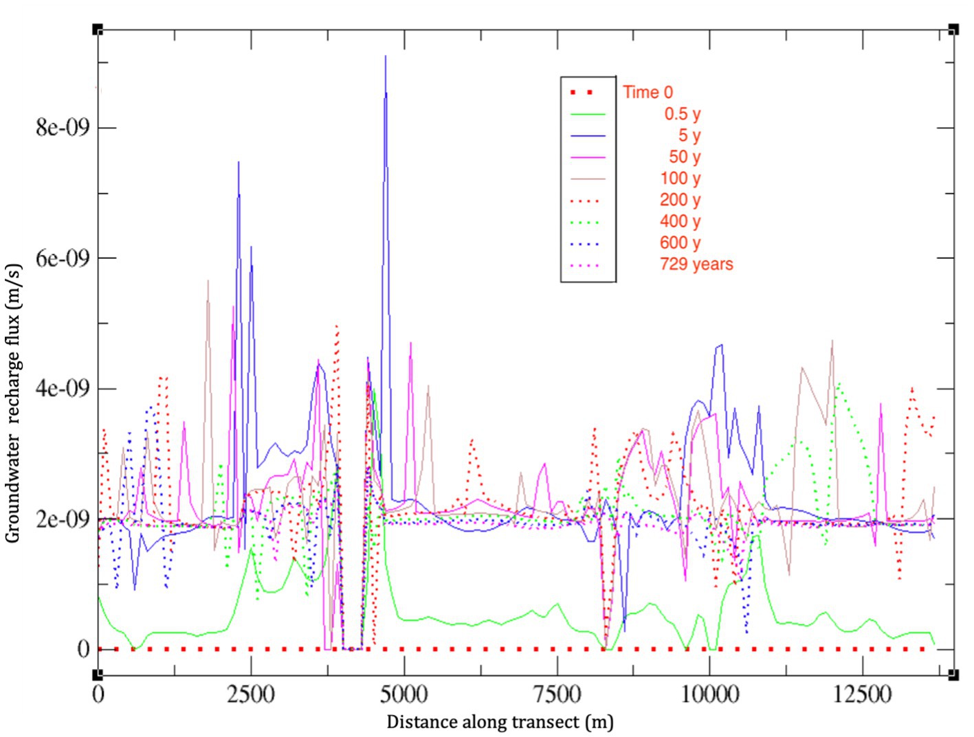
Figure 11. Spatial distribution of groundwater recharge flux computed by CATHY for the 729-year simulation.

Figure 12

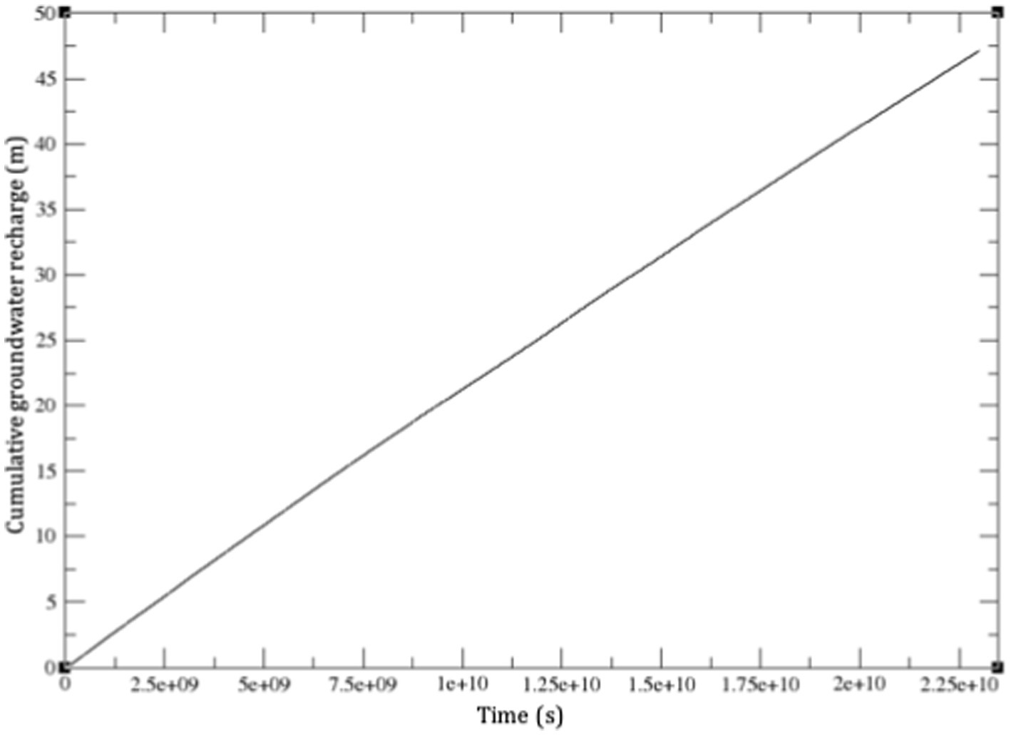
Figure 12. Cumulative (over space and time) groundwater recharge computed by CATHY for the 729-year simulation.

3.2.3 Spatial and temporal discretization challenges

Much attention in subsurface and coupled surface–subsurface flow modeling is devoted to issues of spatial grid resolution and temporal discretization (e.g., Dawson et al., 2004; Sulis et al., 2011; Liggett et al., 2012; Lipnikov et al., 2016), which is understandable given the complexities of resolving such highly nonlinear and strongly coupled systems whose processes also typically evolve at widely differing characteristic scales. There is thus much scope in CATHY and other ISSHMs for improving discretization schemes, linearization and coupling algorithms, and the accuracy of groundwater velocity and other fluxes that are important derivatives of the primary variable calculations, essential for incorporating solute transport, soil–plant interactions, and other phenomena (e.g., Keyes et al., 2013; Scudeler et al., 2016b).

On this note, we will conclude the Tony Creek transect example with two illustrations of the numerical issues that can arise from spatial and temporal discretizations. As alluded to at the beginning of the previous section (point c), there was indeed an apparent maximum time step size, Δt, that could be achieved for these runs, and this limit or threshold was quite different for the two values of specific storage coefficient: a Δt on the order of 50 min was the upper limit for the run with S_s = 8.1 × 10⁻⁵ m⁻¹, while for the S_s = 0.01 m⁻¹ case it was approximately 3.5 d. Similar outcomes were obtained using other S_s values. Interestingly, the Δt and S_s ratios for these two cases are both around 100, indicating a possible linear scaling relationship.

Figure 13 shows the behavior of the adaptive time stepping scheme used in CATHY (D’Haese et al., 2007) during a very narrow time interval of one of the transect simulations. In CATHY, as well as many other Richards equation-based models, the time step size is allowed to gradually increase so long as the iterative procedure used to solve (linearize) the equation converges rapidly. When convergence difficulties are encountered, on the other hand, the solution procedure performs a “back step,” wherein the time step is repeated with a much smaller Δt. The pattern shown in Figure 13 occurs repeatedly over the course of a simulation, and adds an additional constraining factor to the model’s computational efficiency, on top of the more familiar control on Δt exerted by the temporal resolution and degree of variability in the atmospheric forcing inputs.

Figure 13

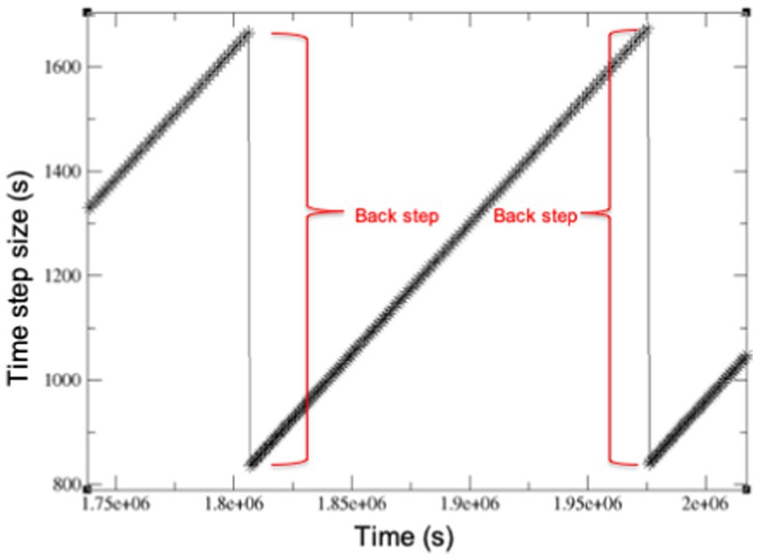
Figure 13. Adaptive time stepping (each “*” is a time step) with two back step occurrences shown for a short time interval extracted from a Tony Creek transect simulation.

There are additional considerations on this issue that warrant attention. When variably saturated conditions prevail, as in the cases examined here, where the water table drops significantly over the course of the simulation (see Figure 10), S_s is not the only storage parameter involved. The general storage term in variably saturated flow models based on Richards’ equation contains also the specific soil moisture capacity (dθ/dψ, where θ is moisture content and ψ is pressure head) and the porosity, and these parameters would presumably also affect time step behavior. Furthermore, as mentioned earlier, the intuitive connection between larger S_s and slower dynamics is predicated on a linear equation (saturated groundwater flow); the behavior under (strongly) nonlinear conditions (e.g., a continually dropping water table) is not as intuitive. Heterogeneity, not addressed in the tests presented here (see Gauthier et al., 2009 for a CATHY-related example), would likely complicate matters further if, in addition to hydraulic conductivity, storage parameters are also spatially variable.

With regard to spatial discretization, it is generally advisable, when dealing with 2D and 3D domains, to avoid highly distorted elements within a computational grid, as these can lead to solver convergence problems and solution inaccuracies. In integrated surface water–groundwater modeling, mesh skewness typically arises in discretizing steep terrain, but it can occur also over relatively flat terrain where distortion is accentuated by very high aspect ratios between the horizontal and vertical discretizations, especially when applying ISSHMs at large spatial scales. This is illustrated in Figure 14 for the Tony Creek transect. As mentioned in Section 2.2, the average terrain slope on each side of the Tony Creek transect is quite mild (~1.7%). Even locally, the steepest slope, along the right streambank, reaches only 6.8%. (This is in contrast, for instance, to the much steeper terrain gradient for the LEO hillslope, of 17.6%.) However, the 20 m horizontal grid size used for the Tony Creek transect, combined with a 15 cm vertical grid size for the critical topmost layer, results in an aspect ratio Δx/Δz of 133. For an average slope of 1.7%, this gives a vertical drop of 34 cm over a 20 m lateral distance, which is more than double the layer thickness. Where the terrain is locally steeper the drop is much greater, as shown in Figure 14.

Figure 14

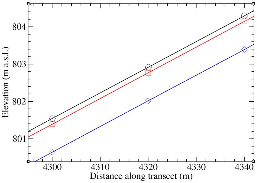
Figure 14. Zoom on two cells (Δx = 20 m for both) and 2 layers (Δz = 15 cm between the black and red lines that demarcate the topmost layer; Δz = 75 cm between the red and blue lines demarcating the second layer) of the Tony Creek transect discretization.

In the simulations presented for this study, we did not conduct a detailed analysis of aspect ratio impacts, to the extent for example of attributing specific numerical problems observed to mesh distortion versus other factors, but it is certainly an issue that warrants further attention in the context of integrated hydrological modeling. An aspect ratio of 133 was not considered unreasonable in view of a prior study (Paniconi and Wood, 1993) where satisfactory results were obtained with aspect ratios as high as 150, provided the convergence criterion on the iterative solver for Richards’ equation was not too stringent. Calver and Wood (1989), on the other hand, recommended stricter limits on aspect ratio (Δx/Δz ≤ 20) for subsurface flow models. There can be significant trade-offs between keeping computational costs low (large aspect ratios) and maintaining accurate numerical solutions (small aspect ratios), as investigated for instance by Badrot-Nico et al. (2007) for the advection–diffusion equation. In addition to imposing limits on the spatial grid, the fine vertical grid spacing typically used for near-surface layers in order to resolve flux partitioning also restricts the temporal discretization, adding another facet to the accuracy–cost trade-off. There is a need to extend analysis of these issues to ISSHMs, as coupling may introduce additional factors that constrain mesh aspect ratios. In the specific case of CATHY and other DEM-based ISSHMs, another limitation arises from the use of a nonuniform surface grid. Mesh refinement where the terrain is steeper would allow for smaller aspect ratios without unduly amplifying computational costs. This is an important research topic for this class of ISSHMs.

4 Conclusion

Through the small-scale hillslope and large-scale transect examples examined in this paper, we have highlighted some numerical issues that can occur in integrated hydrological modeling, and we have illustrated some of the unexpected or anomalous responses that can arise in simulating such strongly coupled, nonlinear systems. In the LEO hillslope test case, we showed that although qualitatively similar results can be obtained in the capture of flux partitioning across the land surface boundary between coupled and uncoupled runs of the model, the fine details (for, e.g., timing and duration of overland flow) can be quite different. Moreover, there are phenomena that cannot be reproduced without properly resolving surface–subsurface interactions, such as enhanced ponding due to the interplay between the infiltration excess and saturation excess mechanisms of runoff generation. A general point that was emphasized through both the hillslope and transect examples is that correct tracking, including in a mass balance sense, of surface water–groundwater interactions is very challenging, and there is much scope for future research on this central constituent of ISSHMs.

In the Tony Creek transect test case, we showed that, in subsurface-only mode, similar responses for key fluxes at the land surface are reproduced in simulations with and without “guideposts” such as seepage face or Dirichlet boundary conditions placed at or along the stream. However, the responses obtained in coupled mode are significantly different, illustrating the important contribution made by interactions across the land surface that can occur in a continuous or recycled manner, such as downslope reinfiltration. Moreover, it was pointed out that care must be taken when assigning Dirichlet BCs at the surface, in order to avoid unintended (non-physical) sources or sinks of water. In further simulations of the Tony Creek transect, we explored the nature of steady state flow under the flow conditions that prevailed in these runs, featuring strong coupling (exemplified for instance by persistent land surface saturation and high levels of localized ponding) and an expanding unsaturated zone (exemplified by a continually dropping water table). It was observed that if any semblance of a steady state did emerge in this nonlinear flow system, it was in any case highly dependent on the response variable being examined. In these steady state trials, it was moreover found that there was a sustained upper limit to the allowable time step size for any run, and that this upper limit depended strongly on the value of the specific storage coefficient parameter. Thus time stepping is constrained not just by factors such as the temporal resolution and variability of atmospheric (and any other) forcing terms and the strength of coupling and nonlinearity, but also by parameters controlling the internal dynamics of the system such as storage coefficients. Finally, in the transect simulations we suggested that grid aspect ratio issues can arise not just in modeling very steep terrain, but also gently sloping terrain, in particular for large-scale applications.

In addition to challenges associated with complex boundary conditions, mesh irregularities (skewness and aspect ratio), and the resolution and tracking of surface water–groundwater interactions, attention to improving linearization schemes (variants and adaptations of standard Picard and Newton iteration) and refining the substepping scheme in the surface routing module (for, e.g., using more flexible and adaptive criteria linked to ponding levels) are required to ensure robust and accurate results from ISSHM simulations. For models like CATHY, further theoretical development and testing of the boundary condition switching algorithm is needed, and the idea of adding another level of nesting to the model, namely iterative coupling between the surface and subsurface solvers, should be explored.

Overall, it is hoped that the results from the test cases presented in this study have provided some guidelines for further improvements to the coupling and discretization schemes used in ISSHMs. There is no doubt moreover that new numerical issues will emerge as physics-based integrated hydrological models continue to evolve and expand, to more fully include vegetation processes (e.g., Manoli et al., 2014; Brunetti et al., 2019) and ecohydrology in a broad sense (e.g., Niu et al., 2014b; Guswa et al., 2020), and as these models are pushed to ever larger scale applications (Lemieux et al., 2008; Ala-Aho et al., 2015).

Data availability statement

The raw data supporting the conclusions of this article will be made available by the authors, without undue reservation.

Author contributions

CP: Conceptualization, Formal analysis, Investigation, Methodology, Writing – original draft, Writing – review & editing. CL: Conceptualization, Investigation, Writing – review & editing. CR: Conceptualization, Investigation, Writing – review & editing.

Funding

The author(s) declare that no financial support was received for the research and/or publication of this article.

Conflict of interest

The authors declare that the research was conducted in the absence of any commercial or financial relationships that could be construed as a potential conflict of interest.

Generative AI statement

The authors declare that no Gen AI was used in the creation of this manuscript.

Publisher’s note

All claims expressed in this article are solely those of the authors and do not necessarily represent those of their affiliated organizations, or those of the publisher, the editors and the reviewers. Any product that may be evaluated in this article, or claim that may be made by its manufacturer, is not guaranteed or endorsed by the publisher.

Footnotes

1. ^Meneses-Vega, B. J., Paniconi, C., Rivard, C., and Guarin-Martinez, L. I. (under review). A multi-model study of the subsurface and surface hydrodynamics of a 700 km² watershed in western Canada (Fox Creek area, Alberta). J. Hydrol. Reg. Stu.

1. ^Camporese, M., Paniconi, C., and Putti, M. (under review). Groundwater recharge is not the whole story: saturated storage dynamics provides a complete picture of subsurface water availability. Water Resources Res.

References

Ala-Aho, P., Rossi, P. M., Isokangas, E., and Kløve, B. (2015). Fully integrated surface–subsurface flow modelling of groundwater–lake interaction in an esker aquifer: model verification with stable isotopes and airborne thermal imaging. J. Hydrol. 522, 391–406. doi: 10.1016/j.jhydrol.2014.12.054

Crossref Full Text | Google Scholar

Badrot-Nico, F., Brissaud, F., and Guinot, V. (2007). A finite volume upwind scheme for the solution of the linear advection–diffusion equation with sharp gradients in multiple dimensions. Adv. Water Resour. 30, 2002–2025. doi: 10.1016/j.advwatres.2007.04.003

Crossref Full Text | Google Scholar

Brunetti, G., Kodešová, R., and Šimůnek, J. (2019). Modeling the translocation and transformation of chemicals in the soil-plant continuum: a dynamic plant uptake module for the HYDRUS model. Water Resour. Res. 55, 8967–8989. doi: 10.1029/2019WR025432

Crossref Full Text | Google Scholar

Calver, A., and Wood, W. L. (1989). On the discretization and cost-effectiveness of a finite element solution for hillslope subsurface flow. J. Hydrol. 110, 165–179. doi: 10.1016/0022-1694(89)90242-4

Crossref Full Text | Google Scholar

Camporese, M., Paniconi, C., Putti, M., and Orlandini, S. (2010). Surface–subsurface flow modeling with path-based runoff routing, boundary condition-based coupling, and assimilation of multisource observation data. Water Resour. Res. 46:W02512. doi: 10.1029/2008WR007536

PubMed Abstract | Crossref Full Text | Google Scholar

D’Haese, C. M. F., Putti, M., Paniconi, C., and Verhoest, N. E. C. (2007). Assessment of adaptive and heuristic time stepping for variably saturated flow. Int. J. Numer. Methods Fluids 53, 1173–1193. doi: 10.1002/fld.1369

Crossref Full Text | Google Scholar

Dagès, C., Paniconi, C., and Sulis, M. (2012). Analysis of coupling errors in a physically-based integrated surface water–groundwater model. Adv. Water Resour. 49, 86–96. doi: 10.1016/j.advwatres.2012.07.019

Crossref Full Text | Google Scholar

Dawson, C., Sun, S., and Wheeler, M. F. (2004). Compatible algorithms for coupled flow and transport. Comput. Methods Appl. Mech. Eng. 193, 2565–2580. doi: 10.1016/j.cma.2003.12.059

Crossref Full Text | Google Scholar

Discacciati, M., Miglio, E., and Quarteroni, A. (2002). Mathematical and numerical models for coupling surface and groundwater flows. Appl. Numer. Math. 43, 57–74. doi: 10.1016/S0168-9274(02)00125-3

Crossref Full Text | Google Scholar

Farthing, M. W., and Ogden, F. L. (2017). Numerical solution of Richards' equation: a review of advances and challenges. Soil Sci. Soc. Am. J. 81, 1257–1269. doi: 10.2136/sssaj2017.02.0058

Crossref Full Text | Google Scholar

Fiorentini, M., Orlandini, S., and Paniconi, C. (2015). Control of coupling mass balance error in a process-based numerical model of surface–subsurface flow interaction. Water Resour. Res. 51, 5698–5716. doi: 10.1002/2014WR016816

Crossref Full Text | Google Scholar

Furman, A. (2008). Modeling coupled surface–subsurface flow processes: a review. Vadose Zone J. 7, 741–756. doi: 10.2136/vzj2007.0065

Crossref Full Text | Google Scholar

Gatel, L., Lauvernet, C., Carluer, N., Weill, S., and Paniconi, C. (2020). Sobol global sensitivity analysis of a coupled surface/subsurface water flow and reactive solute transfer model on a real hillslope. Water 12:121. doi: 10.3390/w12010121

PubMed Abstract | Crossref Full Text | Google Scholar

Gatto, B., Paniconi, C., Salandin, P., and Camporese, M. (2021). Numerical dispersion of solute transport in an integrated surface–subsurface hydrological model. Adv. Water Resour. 158:104060. doi: 10.1016/j.advwatres.2021.104060

Crossref Full Text | Google Scholar

Gauthier, M.-J., Camporese, M., Rivard, C., Paniconi, C., and Larocque, M. (2009). A modeling study of heterogeneity and surface water–groundwater interactions in the Thomas brook catchment, Annapolis Valley (Nova Scotia, Canada). Hydrol. Earth Syst. Sci. 13, 1583–1596. doi: 10.5194/hess-13-1583-2009

Crossref Full Text | Google Scholar

Guswa, A. J., Tetzlaff, D., Selker, J. S., Carlyle-Moses, D. E., Boyer, E. W., Bruen, M., et al. (2020). Advancing ecohydrology in the 21st century: a convergence of opportunities. Ecohydrology 13:e2208. doi: 10.1002/eco.2208

Crossref Full Text | Google Scholar

Haque, A., Salama, A., Lo, K., and Wu, P. (2021). Surface and groundwater interactions: a review of coupling strategies in detailed domain models. Hydrology 8:35. doi: 10.3390/hydrology8010035

Crossref Full Text | Google Scholar

Irvine, D. J., Singha, K., Kurylyk, B. L., Briggs, M. A., Sebastian, Y., Tait, D. R., et al. (2024). Groundwater-surface water interactions research: past trends and future directions. J. Hydrol. 644:132061. doi: 10.1016/j.jhydrol.2024.132061

Crossref Full Text | Google Scholar

Kelley, C. T. (1995). Iterative methods for linear and nonlinear equations. Philadelphia, PA: Society for Industrial and Applied Mathematics.

Google Scholar

Keyes, D. E., McInnes, L. C., Woodward, C., Gropp, W., Myra, E., Pernice, M., et al. (2013). Multiphysics simulations: challenges and opportunities. Int. J. High Perf. Comput. Appl. 27, 4–83. doi: 10.1177/1094342012468181

Crossref Full Text | Google Scholar

Kollet, S., Sulis, M., Maxwell, R. M., Paniconi, C., Putti, M., Bertoldi, G., et al. (2017). The integrated hydrologic model intercomparison project, IH-MIP2: a second set of benchmark results to diagnose integrated hydrology and feedbacks. Water Resour. Res. 53, 867–890. doi: 10.1002/2016WR019191

Crossref Full Text | Google Scholar

Lemieux, J. M., Sudicky, E. A., Peltier, W. R., and Tarasov, L. (2008). Dynamics of groundwater recharge and seepage over the Canadian landscape during the Wisconsinian glaciation. J. Geophys. Res. 113:F01011. doi: 10.1029/2007JF000838

PubMed Abstract | Crossref Full Text | Google Scholar

Liggett, J. E., Werner, A. D., and Simmons, C. T. (2012). Influence of the first-order exchange coefficient on simulation of coupled surface–subsurface flow. J. Hydrol. 415, 503–515. doi: 10.1016/j.jhydrol.2011.11.028

PubMed Abstract | Crossref Full Text | Google Scholar

Lipnikov, K., Konstantin, L., David, M., and Daniil, S. (2016). New preconditioning strategy for Jacobian-free solvers for variably saturated flows with Richards’ equation. Adv. Water Resour. 94, 11–22. doi: 10.1016/j.advwatres.2016.04.016

Crossref Full Text | Google Scholar

List, F., and Radu, F. A. (2016). A study on iterative methods for solving Richards’ equation. Comput. Geosci. 20, 341–353. doi: 10.1007/s10596-016-9566-3

Crossref Full Text | Google Scholar

Manoli, G., Bonetti, S., Domec, J.-C., Putti, M., Katul, G., and Marani, M. (2014). Tree root systems competing for soil moisture in a 3D soil–plant model. Adv. Water Resour. 66, 32–42. doi: 10.1016/j.advwatres.2014.01.006

Crossref Full Text | Google Scholar

Maxwell, R. M., Putti, M., Meyerhoff, S., Delfs, J.-O., Ferguson, I. M., Ivanov, V., et al. (2014). Surface–subsurface model intercomparison: a first set of benchmark results to diagnose integrated hydrology and feedbacks. Water Resour. Res. 50, 1531–1549. doi: 10.1002/2013WR013725

Crossref Full Text | Google Scholar

Miller, C. T., Dawson, C. N., Farthing, M. W., Hou, T. Y., Huang, J., Kees, C. E., et al. (2013). Numerical simulation of water resources problems: models, methods, and trends. Adv. Water Resour. 51, 405–437. doi: 10.1016/j.advwatres.2012.05.008

Crossref Full Text | Google Scholar

Niu, G.-Y., Paniconi, C., Troch, P. A., Scott, R. L., Durcik, M., Zeng, X., et al. (2014b). An integrated modelling framework of catchment-scale ecohydrological processes: 1. Model description and tests over an energy-limited watershed. Ecohydrology 7, 427–439. doi: 10.1002/eco.1362

Crossref Full Text | Google Scholar

Niu, G.-Y., Pasetto, D., Scudeler, C., Paniconi, C., Putti, M., Troch, P. A., et al. (2014a). Incipient subsurface heterogeneity and its effect on overland flow generation – insight from a modeling study of the first experiment at the biosphere 2 landscape evolution observatory. Hydrol. Earth Syst. Sci. 18, 1873–1883. doi: 10.5194/hess-18-1873-2014

Crossref Full Text | Google Scholar

Omar, P. J., Shivhare, N., Dwivedi, S. B., Gaur, S., and Dikshit, P. K. S. (2021). “Study of methods available for groundwater and surface water interaction: a case study on Varanasi, India” in The Ganga River basin: A Hydrometeorological approach. eds. M. S. Chauhan and C. S. P. Ojha (Cham: Springer), 67–83.

Google Scholar

Orlandini, S., and Moretti, G. (2009). Determination of surface flow paths from gridded elevation data. Water Resour. Res. 45:W03417. doi: 10.1029/2008WR007099

PubMed Abstract | Crossref Full Text | Google Scholar

Orlandini, S., Moretti, G., Franchini, M., Aldighieri, B., and Testa, B. (2003). Path-based methods for the determination of nondispersive drainage directions in grid-based digital elevation models. Water Resour. Res. 39:1144. doi: 10.1029/2002WR001639

PubMed Abstract | Crossref Full Text | Google Scholar

Özgen-Xian, I., Molins, S., Johnson, R. M., Xu, Z., Dwivedi, D., Loritz, R., et al. (2023). Understanding the hydrological response of a headwater-dominated catchment by analysis of distributed surface–subsurface interactions. Sci. Rep. 13:4669. doi: 10.1038/s41598-023-31925-w

PubMed Abstract | Crossref Full Text | Google Scholar

Paniconi, C., Aldama, A. A., and Wood, E. F. (1991). Numerical evaluation of iterative and noniterative methods for the solution of the nonlinear Richards equation. Water Resour. Res. 27, 1147–1163. doi: 10.1029/91WR00334

Crossref Full Text | Google Scholar

Paniconi, C., and Putti, M. (2015). Physically based modeling in catchment hydrology at 50: survey and outlook. Water Resour. Res. 51, 7090–7129. doi: 10.1002/2015WR017780

Crossref Full Text | Google Scholar

Paniconi, C., and Wood, E. F. (1993). A detailed model for simulation of catchment scale subsurface hydrologic processes. Water Resour. Res. 29, 1601–1620. doi: 10.1029/92WR02333

Crossref Full Text | Google Scholar

Pasetto, D., Niu, G.-Y., Pangle, L., Paniconi, C., Putti, M., and Troch, P. A. (2015). Impact of sensor failure on the observability of flow dynamics at the biosphere 2 LEO hillslopes. Adv. Water Resour. 86, 327–339. doi: 10.1016/j.advwatres.2015.04.014

Crossref Full Text | Google Scholar

Putti, M., and Paniconi, C. (2004). Time step and stability control for a coupled model of surface and subsurface flow. Dev. Water Sci. 55, 1391–1402. doi: 10.1016/S0167-5648(04)80152-7

Crossref Full Text | Google Scholar

Sanchez-Vila, X., Guadagnini, A., and Carrera, J. (2006). Representative hydraulic conductivities in saturated groundwater flow. Rev. Geophys. 44:RG3002. doi: 10.1029/2005RG000169

PubMed Abstract | Crossref Full Text | Google Scholar

Scudeler, C., Pangle, L., Pasetto, D., Niu, G.-Y., Volkmann, T., Paniconi, C., et al. (2016a). Multiresponse modeling of variably saturated flow and isotope tracer transport for a hillslope experiment at the landscape evolution observatory. Hydrol. Earth Syst. Sci. 20, 4061–4078. doi: 10.5194/hess-20-4061-2016

Crossref Full Text | Google Scholar

Scudeler, C., Paniconi, C., Pasetto, D., and Putti, M. (2017). Examination of the seepage face boundary condition in subsurface and coupled surface/subsurface hydrological models. Water Resour. Res. 53, 1799–1819. doi: 10.1002/2016WR019277

Crossref Full Text | Google Scholar

Scudeler, C., Putti, M., and Paniconi, C. (2016b). Mass-conservative reconstruction of Galerkin velocity fields for transport simulations. Adv. Water Resour. 94, 470–485. doi: 10.1016/j.advwatres.2016.06.011

Crossref Full Text | Google Scholar

Senatore, A., Micieli, M., Liotti, A., Durighetto, N., Mendicino, G., and Botter, G. (2021). Monitoring and modeling drainage network contraction and dry down in Mediterranean headwater catchments. Water Resour. Res. 57:e2020WR028741. doi: 10.1029/2020WR028741

PubMed Abstract | Crossref Full Text | Google Scholar

Sochala, P., Ern, A., and Piperno, S. (2009). Mass conservative BDF-discontinuous Galerkin/explicit finite volume schemes for coupling subsurface and overland flows. Comput. Methods Appl. Mech. Eng. 198, 2122–2136. doi: 10.1016/j.cma.2009.02.024

Crossref Full Text | Google Scholar

Stokke, J. S., Mitra, K., Storvik, E., Both, J. W., and Radu, F. A. (2023). An adaptive solution strategy for Richards’ equation. Comput. Mathematics Appl. 152, 155–167. doi: 10.1016/j.camwa.2023.10.020

Crossref Full Text | Google Scholar

Sulis, M., Meyerhoff, S. B., Paniconi, C., Maxwell, R. M., Putti, M., and Kollet, S. J. (2010). A comparison of two physics-based numerical models for simulating surface water–groundwater interactions. Adv. Water Resour. 33, 456–467. doi: 10.1016/j.advwatres.2010.01.010

Crossref Full Text | Google Scholar

Sulis, M., Paniconi, C., and Camporese, M. (2011). Impact of grid resolution on the integrated and distributed response of a coupled surface–subsurface hydrological model for the des Anglais catchment, Quebec. Hydrol. Proc. 25, 1853–1865. doi: 10.1002/hyp.7941

Crossref Full Text | Google Scholar

van Genuchten, M. T. (1980). A closed-form equation for predicting the hydraulic conductivity of unsaturated soils. Soil Sci. Soc. Am. J. 44, 892–898. doi: 10.2136/sssaj1980.03615995004400050002x

Crossref Full Text | Google Scholar

Vereecken, H., Schnepf, A., Hopmans, J. W., Javaux, M., Or, D., Roose, T., et al. (2016). Modeling soil processes: review, key challenges, and new perspectives. Vadose Zone J. 15, 1–57. doi: 10.2136/vzj2015.09.0131

Crossref Full Text | Google Scholar

Waldowski, B., Sánchez-León, E., Cirpka, O. A., Brandhorst, N., Hendricks Franssen, H.-J., and Neuweiler, I. (2023). Estimating groundwater recharge in fully integrated pde-based hydrological models. Water Resour. Res. 59:e2022WR032430. doi: 10.1029/2022WR032430

Crossref Full Text | Google Scholar

Ward, A. S., Schmadel, N. M., and Wondzell, S. M. (2018). Simulation of dynamic expansion, contraction, and connectivity in a mountain stream network. Adv. Water Resour. 114, 64–82. doi: 10.1016/j.advwatres.2018.01.018

Crossref Full Text | Google Scholar

Weill, S., Mazzia, A., Putti, M., and Paniconi, C. (2011). Coupling water flow and solute transport into a physically-based surface–subsurface hydrological model. Adv. Water Resour. 34, 128–136. doi: 10.1016/j.advwatres.2010.10.001

Crossref Full Text | Google Scholar

Zanetti, F., Camporese, M., and Botter, G. (2024). How do different runoff generation mechanisms drive stream network dynamics? Insights from physics-based modelling. Hydrol. Proc. 38:e15234. doi: 10.1002/hyp.15234

PubMed Abstract | Crossref Full Text | Google Scholar