Abstract
Periods of extreme dry weather and extreme wet weather have stressed water resources worldwide. California’s water management sectors face an increased risk from climate change, and consequently the California Department of Water Resources has investigated the benefits of using floodwater for managed aquifer recharge (Flood-MAR). Flood-MAR requires the implementation of an integrated surface-ground water resources approach that can address watershed hydrologic processes from the atmosphere to the valley floor and the aquifer systems. In this process, it was learned that there is a need to develop a root-zone model with the capability of determining both the amount and the frequency of the applied water at field scale using crop and soil data to avoid damaging agricultural crops. Therefore, the following factors were considered: soil suitability, crop suitability, and soil oxygen depletion due to the application of water available for recharge. IDC (Integrated Demand Calculator) is a stand-alone root zone component of the Integrated Water Flow Model (IWFM) which provides conceptual features for simulating root zone saturation levels. We propose a simple conceptual root-zone model to calculate the application amount and frequency of water available for recharge through the implementation of Flood-MAR operations on agricultural fields. The method is based on soil-land use combination, and crop saturation tolerance considering seasonal patterns during a long-term application of water available for recharge. The results of the conceptual root-zone model were (i) the amount of applied water, (ii) the reached saturation water content in the root zone not exceeding 75 percent saturation to avoid inhibiting plant respiration and growth, (iii) the potential return interval between applications for each soil-land use combination, and (iv) the amount of applied water needed to maintain six inches of ponding water depth in fallow land. The model proved it’s a useful tool for water management in practice where its utility is outstanding, and it provides valuable information to guide planners, water district managers and farmers when implementing Flood-MAR.
1 Introduction
Periods of extreme dry weather and extreme wet weather have stressed water resources worldwide. Climate change is altering California’s water resources, leading to greater variability in weather and hydrology (California Department of Water Resources (CDWR), 2022b). Overall, all water management sectors in California face an increased risk from climate change and in the San Joaquin Valley, water management challenges are intensifying. The San Joaquin Valley already faces severe water management challenges even under current climate conditions, including groundwater overdraft (California Department of Water Resources (CDWR), 2022b; Faunt et al., 2016; Harter, 2015; SGMA, 2025) that is exacerbated by climate change.
The California Water Resilience Portfolio (California Department of Water Resources (CDWR), 2020) prioritized key actions to secure California’s water future, including opportunities to recharge and watershed-scale climate vulnerability and adaptation assessments. California’s Water Supply Strategy (California Department of Water Resources (CDWR), 2022a) also emphasized the opportunities associated with intentional groundwater recharge (i.e., managed aquifer recharge) to harness the bounty of wet years to cope with dry years.
The California Department of Water Resources (CADWR) in partnership with federal, state, and local stakeholders developed the San Joaquin Basin Flood-Managed Aquifer Recharge Watershed Studies (California Department of Water Resources (CDWR), 2024) to investigate the benefits of using floodwater for managed aquifer recharge (Flood-MAR) across five watersheds located in the San Joaquin Basin in California, USA.
Flood-MAR is an integrated and voluntary resource management strategy that can be used to address the risks of a changed climate condition to multiple sectors of water management including flood risk, water supply, and ecosystems (California Department of Water Resources (CDWR), 2018a). Flood-MAR requires the implementation of an integrated surface-ground water resources approach that can address watershed hydrologic processes from the atmosphere to the valley floor and the aquifer systems. To properly analyze and integrate these hydrologic processes, there is a need to deploy different modeling tools. These models simulate current and past conditions and predict future hydro-climatological conditions (California Department of Water Resources (CDWR), 2024). In this process, it was learned that there is a need to develop a root zone model with the capability of determining both the amount and the frequency of the applied water at field scale using crop and soil data.
Several models exist for simulating water flow in the root zone and estimating groundwater recharge. It includes process-based numerical models such as HYDRUS (Šimůnek and van Genuchten, 2008), IDC (Dogrul et al., 2011), and SWAT (Neitsch et al., 2011), integrated models such as MIKE SHE (Abbott et al., 1986a, 1986b) and HydroGeoSphere (Brunner and Simmons, 2012), and hybrid models. Each one of these platforms has their own distinct strengths and applications depending on the scale, complexity, and objectives.
Some numerical models solve governing equations for water flow and transport in the unsaturated and saturated zones at the watershed scale. The first example is HYDRUS (1D/2D/3D) which solves the Richards equation for variably saturated flow and simulates root water uptake, evaporation, and infiltration under complex boundary conditions (Šimůnek and van Genuchten, 2008; Šimůnek et al., 2016). One illustration of Hydrus application in managed aquifer recharge (MAR) is the model developed by Bali et al. (2023), which was used to analyze the net recharge can be applied to alfalfa fields during winter. Other studies also used Hydrus to implement the MAR concept within their study area (Zhou et al., 2023; Sallwey et al., 2018). The next example of numerical models is SWAT (Soil and Water Assessment Tool) which is a semi-distributed model for watershed-scale hydrology, including groundwater recharge. It links recharge with land use and climate variability but has a simplified representation of unsaturated flow (Neitsch et al., 2011; Arnold et al., 2012). One case study of SWAT model implementation in MAR concept is the work by Rath and Hinge (2024), which the model was used as a tool to evaluate and identify suitable sites for MAR potential within a river basin in Bengal. More studies utilized SWAT for decision-making and assessment of aquifer recharge projects (Ehtiat et al., 2018; Gyamfi et al., 2017). Another choice of numerical model is MIKE SHE which is a fully integrated watershed-scale hydrologic simulation model which originally derived from the SHE model (Abbott et al., 1986a, 1986b) and couples surface, unsaturated, and groundwater flow processes for holistic simulations. The modeling framework developed by Martinsen et al. (2022) is a demonstration of a regional study in China which impacts of different water resources management strategies on MAR practices were explored using MIKE-SHE software. The next modeling platform example is HGS (HydroGeoSphere) which models three-dimensional water and solute flow across surface and subsurface systems at watershed scale. It is suitable for detailed studies involving recharge, flow paths, and contaminant transport (Brunner and Simmons, 2012). Also, Coupled Models have been practiced by combining physically based models (e.g., HYDRUS for unsaturated flow) with machine learning or remote sensing tools for parameter estimation (Yu et al., 2022; Liu et al., 2024).
On the other hand, IDC (Integrated Demand Calculator) is a stand-alone root zone component of the Integrated Water Flow Model (IWFM) which provides conceptual features for simulating root zone saturation levels (Dogrul et al., 2011 and California Department of Water Resources (CDWR), 2015b). The components of IDC relevant to Flood-MAR include surface water flow, soil moisture, soil percolation, and groundwater-surface water interaction. Soil saturation and percolation rates in IDC simulates recharge efficiency and help to determine the optimal flood levels and timing for recharge. The IDC model also serves as a vital tool for estimating recharge duration in agricultural flood-MAR operations and balancing recharge potential with crop health. In this context, understanding and controlling recharging duration is essential for minimizing crop stress while maximizing groundwater recharge. By simulating variables like soil saturation, drainage rates, and root zone water retention, IDC model can simulate the water dynamics over time, predicting when fields become saturated and how long flood recharging persists and how frequent the recharge event should be implemented. This is essential for determining the acceptable recharge duration for specific crop types under Flood-MAR projects (Ganot and Dahlke, 2021; Levintal et al., 2022). O’Geen et al., 2015 defined the root zone residence time (RZRT) as the duration that the root-zone can remain saturated (or nearly saturated) during flood or ponding events without causing crop damage.
Effective flood-MAR requires careful planning to achieve maximum recharge benefits without harming crops. The degree to which root zone saturation harms agricultural crops depends on multiple factors, including the soil type, the crop’s sensitivity to low soil oxygen levels, as well as the timing, frequency, and duration of the saturation (Balerdi et al., 2003). For recharge programs that use agricultural fields, the IDC model can simulate different recharge frequencies (e.g., annual, bi-annual) and periods (e.g., winter when crops are dormant) to identify the most suitable times for both recharge and crop health. Specifically, for perennial crops, scheduling recharge events during dormant seasons (e.g., winter) minimizes the risk of stress (Ganot and Dahlke, 2021).
We identified the need to provide a useful tool for water management in practice and here, we propose a simple conceptual root zone model to calculate the application amount and frequency of water available for recharge through the implementation of Flood-MAR operations on agricultural fields. The method is based on soil-land use combination, and crop saturation tolerance considering seasonal patterns during a long-term application of water available for recharge.
The objective of this manuscript is to determine the amount and frequency of applied water using crop and soil data to avoid damaging agricultural crops on a potential Flood-MAR implementation. Therefore, the following factors are considered: soil suitability (O’Geen et al., 2015), crop suitability (Dahlke et al., 2018), and soil oxygen depletion (Bachand et al., 2019) due to the application of water available for recharge.
2 Methods
2.1 Model purpose and description
A conceptual root zone model was developed with the purpose of calculating the amount and frequency of water available for recharge (WAFR) that can be applied to agricultural fields based on soil water content thresholds, crop type, physical soil parameters, and other parameter settings. The IDC model was used and is a stand-alone root zone component of IWFM. Developed by the California Department of Water Resources (CDWR) (2015a), IWFM calculates agricultural and urban water demands. Agricultural water demand is calculated based on climate data, crop types, crop acreages, soil properties, and irrigation methods. IDC computes applied water demands for ponded and non-ponded crops at each defined grid cell under user-specified climatic and irrigation management settings. For all land-use types, precipitation, as well as applied water, if any, is routed through the root zone (Dogrul et al., 2011; California Department of Water Resources (CDWR), 2015b).
IDC is a root zone model that utilizes methods used by irrigation scheduling models to compute root zone flows and water demands from the agricultural field scale level up to river basin level (Dogrul et al., 2011). Precipitation that falls on the ground surface infiltrates into the soil at a rate dictated by the type of ground cover, physical characteristics of the soil and the moisture that is already available in the soil. The portion of the precipitation that is more than the infiltration rate generates surface flow. In IDC, this surface flow is termed as direct runoff. Irrigation of agricultural lands and urban outdoor also generates surface flow. Surface flow due to irrigation is termed as return flows in IDC. Part of the precipitation and irrigation evaporate before infiltrating into the soil. Infiltration due to precipitation and irrigation replenishes the soil moisture in the root zone which is also depleted through plant root uptake for transpiration and additional evaporation from the top layers of the soil. The transpiration through the plants and evaporation from the land surface, as well as the top layers of the soil, are all simulated as single evapotranspiration (ET) term in IDC. IDC only addresses the moisture vertical direction flow. The moisture that stays in the root zone through its bottom boundary is termed as deep percolation. IDC uses the conservation equation for the soil moisture to compute the flow terms mentioned above and to route the soil moisture through the root zone. For each land use type at a grid cell, the conservation equation is applied in the corresponding defined allowable time-step length (California Department of Water Resources (CDWR), 2015b; Dogrul et al., 2011).
IDC is an object-oriented model that consists of (i) input data files, (ii) output data files, (iii) the numerical engine that reads data from input files, computes applied water demands, routes water through the root zone and prints out the results to output files, and (iv) an user interface that utilizes an ASCII text file that allows the user to define input and output files and simulation control data for the numerical engine (Dogrul et al., 2011; California Department of Water Resources (CDWR), 2015b).
The conceptual IDC model that was developed is a grid-cell array with seven columns by six rows, and each grid cell has a total area of one-acre (0.405 ha). The conceptual IDC model was set up so that each grid cell has a specific combination of a crop type (columns) and soil type (rows). Figure 1 shows the model’s setup, crop type, and physical soil properties for six soil types and seven crop types. The land-use and crop type were defined by identifying the top perennial crops from the 2018 Land IQ database (California Department of Water Resources (CDWR), 2018a, 2018b) in the San Joaquin Valley Watershed. The top seven land-use and perennial crop types are alfalfa, almonds, pasture, pistachios, vineyards, walnuts, and idle (or fallow land). Idle includes the idle land (referred to as fallow land hereafter) and the compatible crop land that is fallow during the winter period. These crops are potatoes and sweet potatoes, cotton, and tomatoes. In this fallow land, flood water can be applied during the whole winter season if water flood is available because the land is not used for agriculture. Soil type corresponds to the six Soil Agricultural Groundwater Banking Index (SAGBI) suitability indexes (Excellent, Good, Moderately Good, Moderately Poor, Poor, and Very Poor) (O’Geen et al., 2015) with corresponding physical soil properties needed in IDC and taken from Rawls et al., 1982. The conceptual IDC model setup is shown in Figure 1.
Figure 1
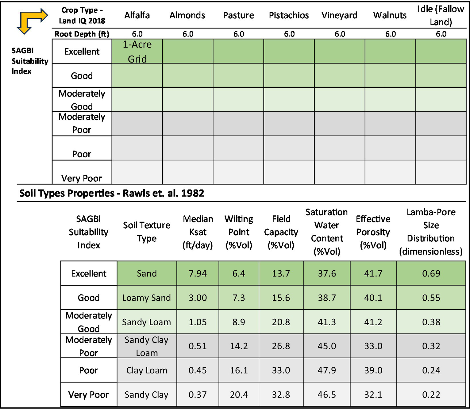
In the top half it is shown the conceptual IDC model set up by crop type (alfalfa, almonds, pasture, pistachios, vineyards, walnuts, and idle) and soil type (SAGBI Suitability Index Soil Types: Excellent, Good, Moderately Good, Moderately Poor, Poor, and Very Poor). In the bottom half it is shown the corresponding physical soil properties implemented in conceptual IDC model. In the Y-axis of the top and bottom half, the soil types properties (Rawls et al., 1982) are shown for corresponding SAGBI Suitability Index.
2.2 Conceptual IDC model assumptions
The conceptual root zone model has six fundamental assumptions that achieve the purpose of its development. These assumptions are described next and all assumptions have the same level of importance.
2.2.1 Assumption 1
In the summer and fall seasons, the soil moisture content starts midway between Field Capacity (FC - amount of water remaining in the soil after excess water has drained away, typically a few days after irrigation or rainfall, representing the upper limit of available water for plant uptake) and Wilting Point (WP - soil moisture level at which plants can no longer extract sufficient water to prevent wilting and will not recover, even when placed in a saturated atmosphere) because of crop production and deficit irrigation practices prior to harvest. In the winter and spring seasons, the soil profile was assumed to be at FC due to the overlapping with the rainy season.
2.2.2 Assumption 2
The WAFR application rate was limited by the potential oxygen decline and set at a threshold of 75 percent saturation to avoid inhibiting plant respiration and growth (Bachand et al., 2019).
2.2.3 Assumption 3
The soil moisture content threshold of FC was established as the threshold growers feel safe to reach before WAFR can be re-applied.
2.2.4 Assumption 4
Based on field experience, it was recommended that the IDC root zone simulations be run to a depth of six feet (1.829 m) which is typically the irrigation management depth of most mature tree crops.
2.2.5 Assumption 5
Conceptual IDC Model assumed six inches (15.24 cm) per day of applied water based on typical turnout capacity for 20-acre (8.094 ha) blocks. The six inches (15.24 cm) water application volume was derived based on field reports that irrigation flow through turnouts is approximately five cubic feet per second (cfs) (0.142 m3/s), the equivalent of 0.5 acre-foot per day (616.74 m3 per day). A 20-acre (8.094 ha) field will therefore accept up to six-acre inches (616.74 m3) of water per day. Additional applied water rates of 10 and 15 cfs (0.283 and 0.425 m3/s) were considered.
2.2.6 Assumption 6
Up to six inches (15.24 cm) of ponding depth in fallow lands. The six inches (15.24 cm) of ponding depth reflects the maximum height of standing water in the field that growers can manage with small field berms.
2.2.7 Underlaying assumptions
The conceptual IDC model was built to determine, based on the amount of applied WAFR, crop type, physical soil properties, and initial soil moisture content, the time it would take for the flood water to percolate and the root zone water content to return to an acceptable level to allow the next application of WAFR. IDC estimates the timing of flood water to infiltrate and to reach a specific soil moisture content threshold (i.e., field capacity) that determines when flood water can be re-applied. This information is transferred to the crop compatibility calendar (CCC) in the Recharge Operation Model, which adjusts the timing for application based on constraints of the crop life cycle (e.g., bloom, dormancy, etc.), field operation (e.g., pruning, timing of fertilizer application), and other practices that protect crop health and crop management. The CCC informs the Recharge Operation Model about how much water can be applied throughout a crop cycle on a daily time-step (Groundwater Recharge Assessment Tool (GRAT), 2025). Precipitation is taken here into account to determine the total potential applied surface water for recharge.
2.3 Spatial and temporal model configuration
2.3.1 Spatial configuration
The spatial configuration in IDC is defined by the “Element” configuration file (Element. DAT) where the configuration for each element represented in the model is defined. For the conceptual IDC model, each element in the grid was defined by a single grid of one-acre (0.405 ha) area. Each element represents a specific combination of crop type and soil type as described in Figure 1. The nodal coordinate file (NodeXY. DAT) contains the node identification number and corresponding X and Y coordinates.
2.3.2 Temporal configuration
To better represent the temporal distribution of input and output datasets, IDC keeps track of the actual date and time of each time-step in a simulation period. Each data entry in the input time series data file is required to have a date and time stamp which allows IDC to retrieve time series data correctly. This, in return, allows the user to maintain a single set of time series input data files for applications, where the starting and ending date and time of the simulation may change. For the conceptual IDC model, one-day time-step length was used.
2.4 Model set-up
2.4.1 Initial soil moisture content
The conceptual IDC model was developed to determine the timing of the re-application of WAFR based on soil types and crop types for the fall, winter, spring and summer seasons. It is known that the water content in the soil profile varies from season to season, so it was decided to use different initial soil water contents depending on the seasons. An initial soil water content of FC was assumed for winter and spring seasons since these seasons overlapped with the rainy season. For the summer and fall seasons when precipitation is mainly absent, the initial soil water content assumed was halfway between WP and FC.
2.4.2 Applied water
The water applied can be defined as the total volume of WAFR applied to agricultural fields per day independently of site suitability (O’Geen et al., 2015), crop suitability (Dahlke et al., 2018), conveyance or agricultural management practices associated with agricultural crops. The depth of water per unit area and per day was defined as six inches (15.24 cm) over five consecutive days. The volume of six inches (15.24 cm) per acre (0.405 ha) of applied water is the result of the turnout’s capacity to deliver water in most of the service areas at the field scale. To input the data into the conceptual IDC model, the “Agricultural Water Supply Requirement” data file was used with a volume of 21,780 cubic feet (616.741 m3) per day (six inches (15.24 cm) per day or 0.5 acre-foot (616.741 m3) per day) over the five consecutive days. However, when the soil water content reaches the threshold of 75 percent saturation (Bachand et al., 2019), applied water starts decreasing to maintain the 75 percent saturation content and avoid inhibiting plant respiration and growth.
2.4.3 Crop evapotranspiration
Crop evapotranspiration (ETc) values for alfalfa, almonds, pasture, pistachios, vineyards, walnuts, and soil evaporation (Okc) for fallow land simulated were determined by the California Simulation of Evapotranspiration of Applied Water (Cal-SIMETAW) model (California Department of Water Resources (CDWR), 2013; Orang et al., 2013) on a daily time step. These Cal-SIMETAW ETc values were validated using the Irrigation Training and Research Center (ITRC) (2012) California Polytechnic State University Evapotranspiration Data for the CIMIS ETo Map Zone 15 Merced (Irrigation Training and Research Center (ITRC) (2012)). The 1998 wet year was used by Cal-SIMETAW and ITRC to compare both datasets. A comparison of both datasets is shown in Figure 2.
Figure 2
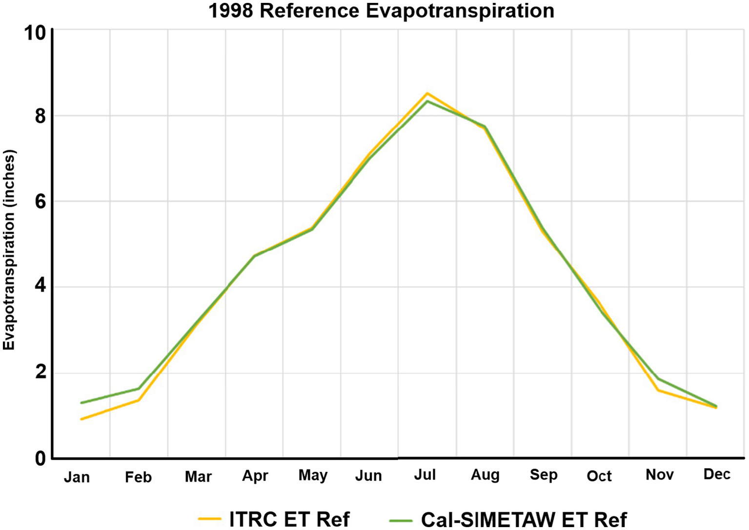
Cal-SIMETAW and ITRC reference evapotranspiration in inches per month (one inch per month equal to 25.4 mm per month) for the 1998 year (wet year).
2.4.4 Land use
To simulate the application of water into agricultural fields without having excess water or surface runoff, the conceptual IDC model was set up to run with non-ponded routines and shifting to ponded routines during specified days. The non-ponded routines are used during most of the year (growing and non-growing seasons) where the soil moisture routing in the root zone is active. During growing and non-growing seasons, perennial crops (alfalfa, almonds, pasture, pistachios, vineyards, and walnuts) are actively growing but also in dormant conditions during wintertime. The shift to ponded conditions happens during specific days that WAFR is applied to agricultural lands. The conceptual IDC model changes to ponded routines to route the soil moisture in the root zone where lands can potentially get saturated or even flooded as described next.
Figure 3 shows a decision chart representation of a hydrological year starting on October 01 and ending on September 30. The conceptual IDC model runs with ponded routines for five consecutive days during the fall (Oct 01–05), winter (Jan 01–05), spring (Apr 01–05), and summer (01–05) seasons when WAFR is applied. The rest of the time the model runs with non-ponded routines. Two input files are used to set up the non-ponded and ponded routines. The “Non-Ponded Crop Area” file (CropAreas.dat) contains the land use distribution of non-ponded (agricultural) crops for each element in the simulation period. Each element associated with each crop and soil type combination is active when there is a coefficient of one (1.0) and non-active when there is a coefficient of zero (0.0) during each time step in the input area file. In Figure 3 the “Non-Ponded Crop Area” file has values of one (1.0) when WAFR is not applied. The “Ponded Crop Area” file (RiceAreas.dat) contains the land distribution for crops when WAFR is applied, and agricultural fields can potentially get flooded. Ponded routines are needed here so WAFR can be ponded, and it does not become excess water or surface runoff that will be drained out of the field domain. In this file, values of one (1.0) are used for those days when WAFR is applied, and zero (0.0) when not applied. As notice, there is an overlap of both files, non-ponded and ponded crop areas, with one land use active with non-ponded routines, and then there is a shift to ponded routines for a few days allowing the applied WAFR to be ponded if needed and then shifting back to non-ponded conditions when WAFR stops adding.
Figure 3
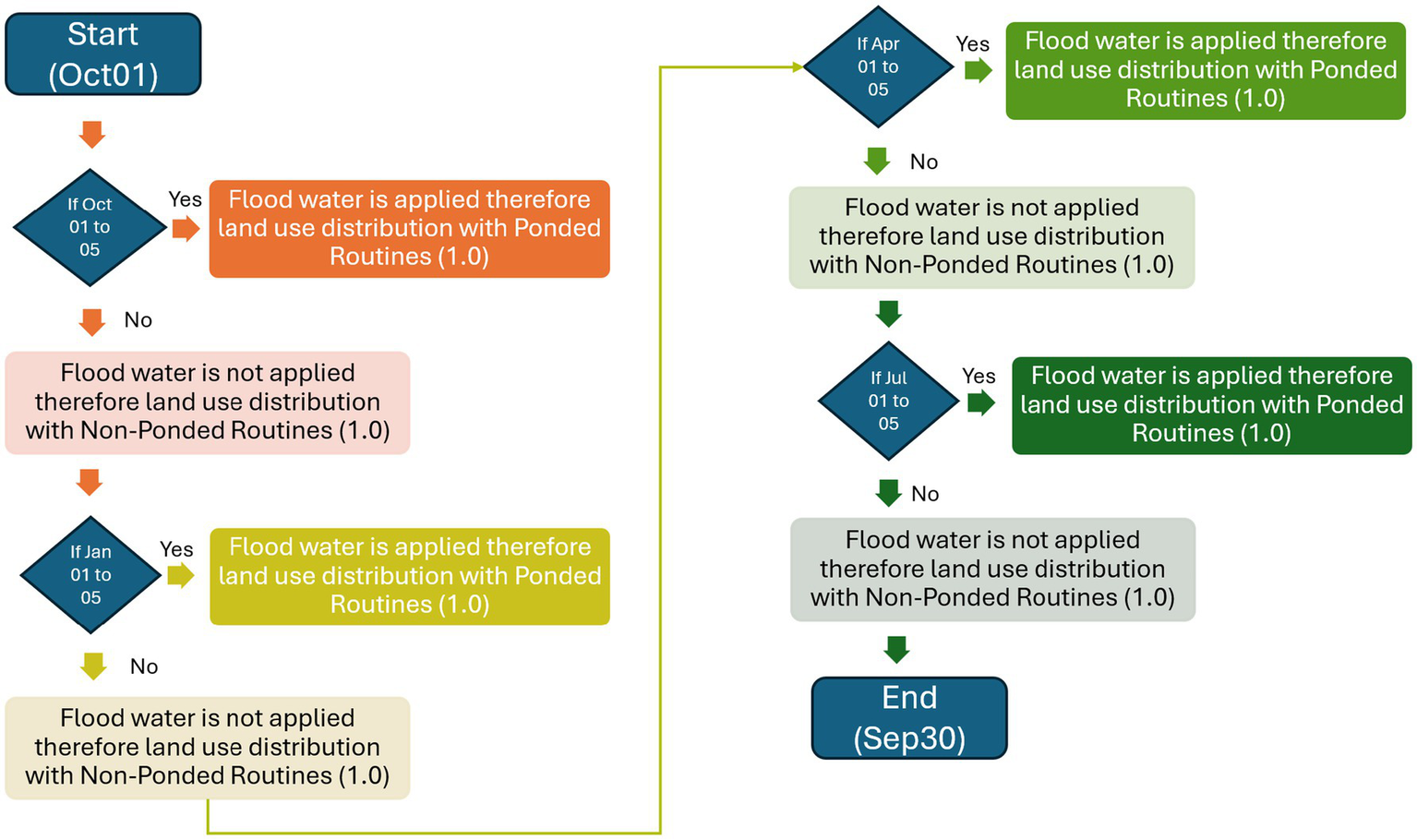
Decision chart representation of a hydrological year (Oct 01 to Sep 30) with implementation of non-ponded routines and ponded routines for soil moisture routing in the root zone.
2.4.5 Precipitation
Precipitation was not considered in the conceptual IDC model. Precipitation is considered in the CCC of the Recharge Operation Model (Groundwater Recharge Assessment Tool (GRAT), 2025) where precipitation is subtracted from the daily total applied WAFR.
3 Results and discussion
3.1 Model output files
The conceptual IDC model produces several optional output files. In the “Root Zone Component Main” file (ROOTZONE_MAIN.dat), the user can specify file names to which soil moisture, land, and water use budgets are printed. These files are created in binary format for run-time efficiency and to save computer storage space. A post-processing tool (Budget) which is available for downloading from the IDC web site is required to process these binary files and create tables in ASCII text file format. Additionally, IDC generates an end-of-simulation moisture content output file that is already in ASCII text format. This file lists soil moisture for each land-use type at each element in the modeling domain (Budget\RootZone.hdf), and it is the output file that was used here to extract IDC results.
The root zone soil moisture file is post-processed in Microsoft Excel using an Add-in tool developed to quickly import data from IDC Budget file into Excel. The root zone soil moisture output file which has units of volume for each land-use type at each element is then processed in Microsoft Excel to get outputs in units of length (inches) per unit area needed in CCC of the Recharge Operation Model (Groundwater Recharge Assessment Tool (GRAT), 2025). This file is a simulation result and has IDC results for each combination of crop type and soil type.
3.2 Model results
Conceptual IDC model result for the almonds crop model with a Moderately Good SAGBI suitability index soil type and five cfs (0.142 m3/s) of applied water is shown in Figure 4. In this example, six inches (15.24 cm) of applied water over one acre (0.405 ha) field per day (equivalent to five cfs (0.142 m3/s)) are applied over five consecutive days (dark blue line) which corresponds to the inputs in the soil moisture mass balance. The outputs are crop evapotranspiration (dash-green line) and the percolation (marron line). The percolation starts at zero on day one and reaches almost six inches (15.24 cm) per day by day five and then gradually decreases over time, eventually returning to zero. The potential return interval (period defined by the end of applied water and when water can be re-applied when ending storage reaches field capacity) between applications is twenty days. It is determined when applied water stops (Day 5) and when the field capacity moisture content threshold is reached (Day 25). In this conceptual IDC model results for almonds, the root zone moisture content (ending storage or magenta line) starts at field capacity because it is winter season (January) on day one, reaches almost 3/4 saturation by day five when applied water stops and starts decreasing gradually. This is the change in storage in the soil moisture mass balance.
Figure 4
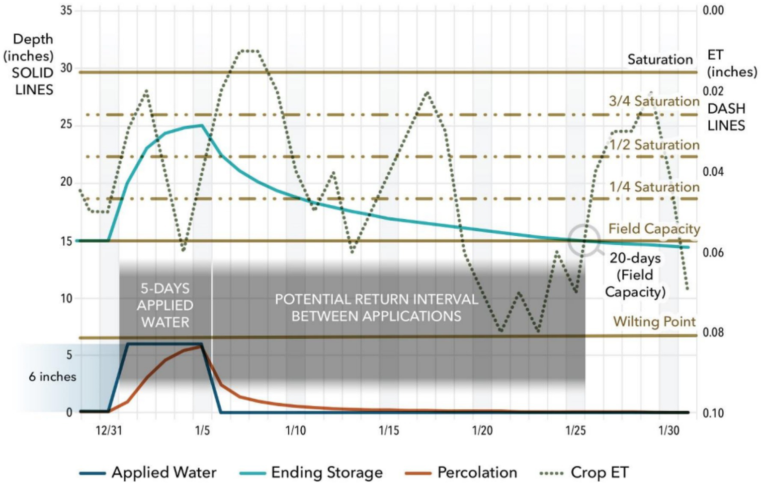
Example of the Conceptual IDC model Results for an Almonds Crop Model with a Moderately Good SAGBI Suitability Index Soil Type and six inches (15.24 cm) per day (five cfs or 0.142 m3/s) of applied water. Six inches (15.24 cm) of water are applied over five (1 to 5) consecutive days (blue line) resulting in percolation (red line) that increases over time reaching a peak by day five. On day six, applied water stops and the percolation rate starts to decrease over time. The initial water soil content (light blue line) for winter time is field capacity since it is the rainy season and it is safe to assume that soils are wet. The ending storage increases over time from day one to day five reaching the highest soil water content on day five, then the ending storage decreases over time since there is not more applied water. Crop evapotranspiration (dash line) occurs and it is variable each day depending on climatological conditions. Applied water is an input, percolation and Crop evapotranspiration are outputs, and ending storage is the change in storage in the conceptual root zone model.
By running the conceptual IDC model and by applying water until the peak soil moisture threshold is reached, average seasonal evapotranspiration and percolation determine how long it would take to reach the field capacity moisture content threshold, so water can be re-applied. The reapplying interval is defined by the physical soil type properties and the specific climate-driven crop evapotranspiration rate. Figure 5 shows an example for the Almonds crop where six inches (15.24 cm) of water depth (five cfs or 0.142 m3/s) of applied water is applied over five consecutive days during the four seasons: fall (October 1–5), winter (January 1–5), spring (April 1–5), and summer (July 1–5).
Figure 5
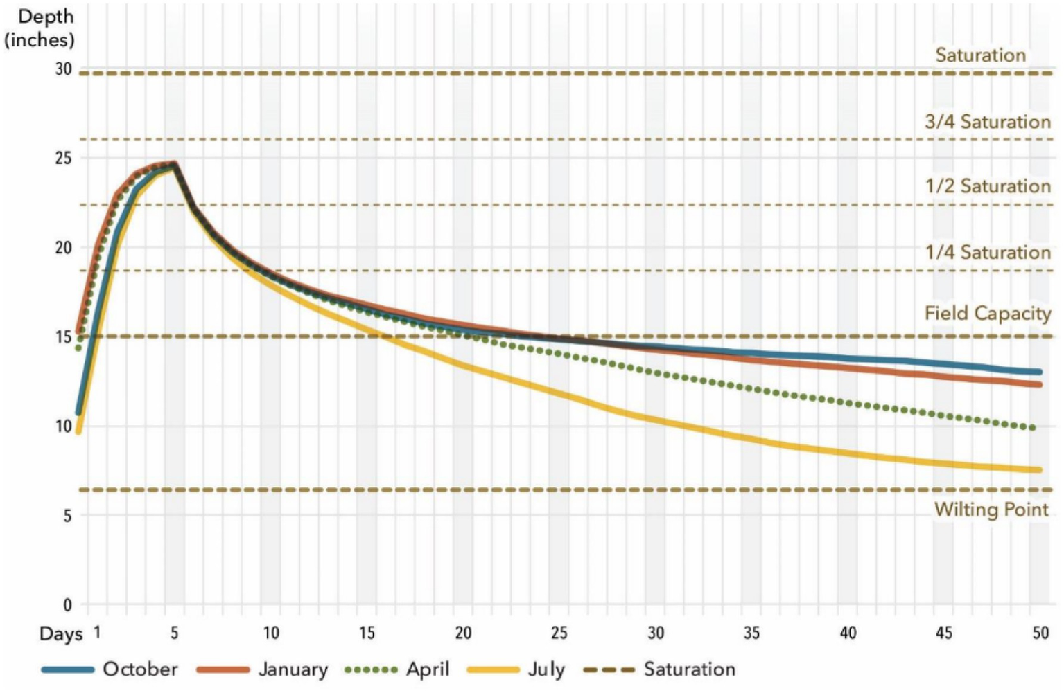
Ending Soil Moisture Content in inches for Almonds crop by seasons October 1–5 (fall), January 1–5 (winter), April 1–5 (spring), and July 1–5 (summer) in a Moderately Good SAGBI Soil Type.
Figure 5 shows that if six inches (15.24 cm) of water depth (equivalent to five cfs or 0.142 m3/s) are applied over five consecutive days, the soil moisture content by day five is almost 3/4 saturation (equivalent to 24.7 inches or 62.7 cm) for the six feet (1.829 m) depth soil profile. At the end of day-five applied water stops. During summer (July), the ending soil moisture content takes approximately 10 days to drain down to reach the field capacity threshold (orange line). During winter (January), the ending soil moisture content takes about 20 days to drain down to reach the field capacity threshold (red line). Spring and fall season intervals are between summer and winter. This interval between when the applied water stops and when the ending soil moisture content reaches field capacity threshold is the potential return interval between applications (see Figure 4).
The potential return interval between applications is used to define the “black-out period” in the CCC of the Recharge Operation Model (Groundwater Recharge Assessment Tool (GRAT), 2025) which is when no additional WAFR is applied to agricultural fields. This black-out period used in the model may be longer than actual practice by farmers who may desire to reapply water or take some risk applying water if WAFR is available. A conservative black-out period can be used in the recharge operation model to avoid overestimating potential recharge although it may result in missing the opportunity to capture more available WAFR (Groundwater Recharge Assessment Tool (GRAT), 2025).
Table 1 shows the potential return interval in days between water applications by crop types (alfalfa, almonds, pasture, pistachios, vineyards, and walnuts) and soil types (SAGBI Suitability Index Soil Types: Excellent, Good, Moderately Good, Moderately Poor, Poor, and Very Poor). When applied water stops, the ending soil moisture content may reach 3/4 saturation or less depending on the SAGBI soil type, and from there, the soil moisture content will drain down until reaching field capacity. The shortest potential return interval is for the Excellent SAGBI soil type as expected. The potential return interval increases gradually for Good, and Moderately Good. However, for Moderately Poor, Poor and Very Poor return intervals get shorter compared to the Moderately Good SAGBI soil type. This is due to the field capacity parameters (Rawls et al., 1982) where sandy type soils have greater field capacity parameters than clay type soils (see Figure 1), thus in the sandy soil types the field capacity threshold is reached sooner. Since Flood-MAR is a multi-benefit approach (California Department of Water Resources (CDWR), 2018a) all six SAGBI soil types are used. The Excellent, Good, and Moderately Good SAGBI soil types have a high infiltration rate, so they are used to achieve maximum recharge benefits mainly on farm recharge programs. Any applied WAFR will infiltrate and eventually percolate quickly making these soil types ideal for Flood-MAR. The Moderately Poor, Poor and Very Poor SAGBI soil types are used to create shorebird habitat where a field must be continuously inundated for 30 days with 2 inches (5.08 cm) of ponding.
Table 1
| SAGBI Soil Type | Seasons | Alfalfa | Almonds | Pasture | Pistachios | Vineyard | Walnuts |
|---|---|---|---|---|---|---|---|
| Excellent | Fall (Oct) | 8 | 8 | 8 | 8 | 9 | 8 |
| Winter (Jan) | 9 | 9 | 9 | 9 | 9 | 9 | |
| Spring (Apr) | 8 | 8 | 8 | 8 | 8 | 8 | |
| Summer (Jul) | 7 | 7 | 7 | 7 | 7 | 7 | |
| Good | Fall (Oct) | 17 | 20 | 18 | 23 | 23 | 19 |
| Winter (Jan) | 20 | 20 | 22 | 20 | 20 | 20 | |
| Spring (Apr) | 15 | 16 | 16 | 17 | 17 | 16 | |
| Summer (Jul) | 13 | 12 | 13 | 13 | 13 | 12 | |
| Moderately Good | Fall (Oct) | 27 | 40 | 30 | 41 | 42 | 40 |
| Winter (Jan) | 33 | 33 | 38 | 33 | 33 | 33 | |
| Spring (Apr) | 22 | 24 | 24 | 26 | 25 | 25 | |
| Summer (Jul) | 18 | 16 | 18 | 18 | 19 | 16 | |
| Moderately Poor | Fall (Oct) | 31 | 39 | 30 | 41 | 41 | 39 |
| Winter (Jan) | 27 | 33 | 38 | 33 | 33 | 33 | |
| Spring (Apr) | 19 | 24 | 24 | 26 | 25 | 25 | |
| Summer (Jul) | 18 | 16 | 18 | 18 | 19 | 16 | |
| Poor | Fall (Oct) | 19 | 23 | 20 | 26 | 27 | 23 |
| Winter (Jan) | 23 | 22 | 24 | 23 | 23 | 23 | |
| Spring (Apr) | 17 | 18 | 18 | 19 | 18 | 18 | |
| Summer (Jul) | 14 | 12 | 14 | 14 | 14 | 13 | |
| Very Poor | Fall (Oct) | 20 | 25 | 21 | 28 | 29 | 24 |
| Winter (Jan) | 24 | 24 | 26 | 24 | 24 | 24 | |
| Spring (Apr) | 17 | 18 | 18 | 14 | 19 | 18 | |
| Summer (Jul) | 13 | 12 | 14 | 14 | 14 | 13 |
Potential return interval in days for applied water by crops (alfalfa, almonds, pasture, pistachios, vineyards, and walnuts) and soil types (SAGBI Suitability Index Soil Types: Excellent, Good, Moderately Good, Moderately Poor, Poor, and Very Poor).
The potential return interval between applications is determined between the day that applied water stops and when the field capacity moisture content threshold is reached.
Results for the conceptual IDC model also include the total applied water in units of length (inches) over five consecutive days (six inches (15.24 cm) per day equivalent to 5 cfs or 0.142 m3/s) and corresponding reached saturation water content in the root zone profile. In sandy soil types such as Excellent and Good SABGI soil types, a total of 30 inches (76.2 cm) of water is applied (color bars in Figure 6), and the reached saturation water content is 40.5 percent for Excellent SAGBI soil type and almost 60 percent for Good SAGBI soil type (see dash-black line in Figure 6). As the sand content starts decreasing and the amount of loam and clay increases, the total amount of applied water decreases as expected. The amount of applied water is about 29 inches (73.66 cm) for the Moderately Good SAGBI soil type and it goes down gradually up to 15 inches (38.1 cm) in the Very Poor SAGBI soil type (color bars in Figure 6). The saturation water content in the Moderately Good, Moderately Poor, Poor and Very Poor SAGBI soil types stay around 75 percent saturation (dash-black line in Figure 6).
Figure 6
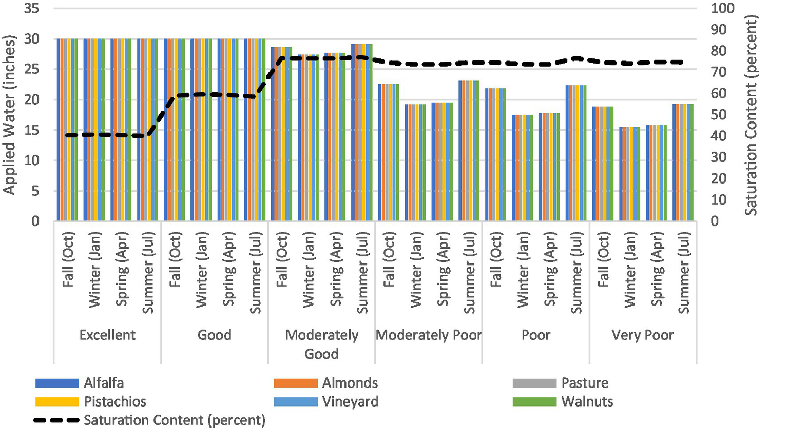
Total applied water in inches for all crops and SAGBI soil types (primary Y-axis) and corresponding reached saturation content as a percent between Soil Saturation and Field Capacity (secondary Y-axis). Applied water delivery was 6 inches (15.24 cm) of water depth per day over 5 consecutive days resulting in 30 inches of applied water in 5 days (six inches (15.24 cm) per day equivalent to 5 cfs or 0.142 m3/s).
A comparison of the conceptual IDC model results against other tools such as the one developed by Ganot and Dahlke (2021) indicates that the recommended conceptual IDC model identified values are in the range of other scientific research results. For example, Ganot and Dahlke (2021) calculated the Ag-MAR flood duration for grapevine assuming an effective root depth of 1-meter (3.28 feet) in a fine sandy loan soil using the RZRT learning tool, and a saturation tolerance of 7-days. The water application duration for Ag-MAR was 6-days and a total water applied of 2.7-meters (8.9 feet). In the conceptual IDC model for vineyard on sandy loam (moderately good SAGBI soil type) with a root depth of six feet (1.83 m), the total applied water over five consecutive days is 27-inches (0.69 m) in winter time and 29-inches (0.74 m) during summer time. Conceptual IDC model results are conservative respect to Ganot and Dahlke (2021) since the total applied water does not exceed the 75 percent saturation while Ganot and Dahlke (2021) saturate the root depth of 1-meter (3.28 feet). This explains the difference in total applied water.
Conceptual IDC model results for fallow land are shown in Figure 7. For Excellent and Good SAGBI soil types up to ninety inches (2.29 m) of water (color bars in Figure 7) can be applied (18 inches (45.7 cm) per day of water depth (15 cfs or 0.425 m3/s). However, no ponding depth can be achieved with this amount of applied water (see black line in Figure 7). This is due to the high content of sand in these corresponding soil types, and it is held up by the physical soil parameters in Figure 1. For Moderately Good, Moderately Poor, Poor, and Very Poor SAGBI soil types a ponding depth of six inches (15.24 cm) is reached (see dash-black line in Figure 7) as it is defined in the model assumptions. The total applied water on those fallow lands starts decreasing from 79 inches (2.01 m) in the Moderately Good to 38 inches (96.5 cm) over five consecutive days in the Very Poor SAGBI soil type. This is the result of higher content of loam and clay in these SAGBI soil types and it is reflected in the physical soil parameters that characterized these SAGBI soil types (see Figure 1). The six inches (15.24 cm) of ponding depth reflects the maximum height of standing water in the fallow land fields that growers can manage with small field berms.
Figure 7
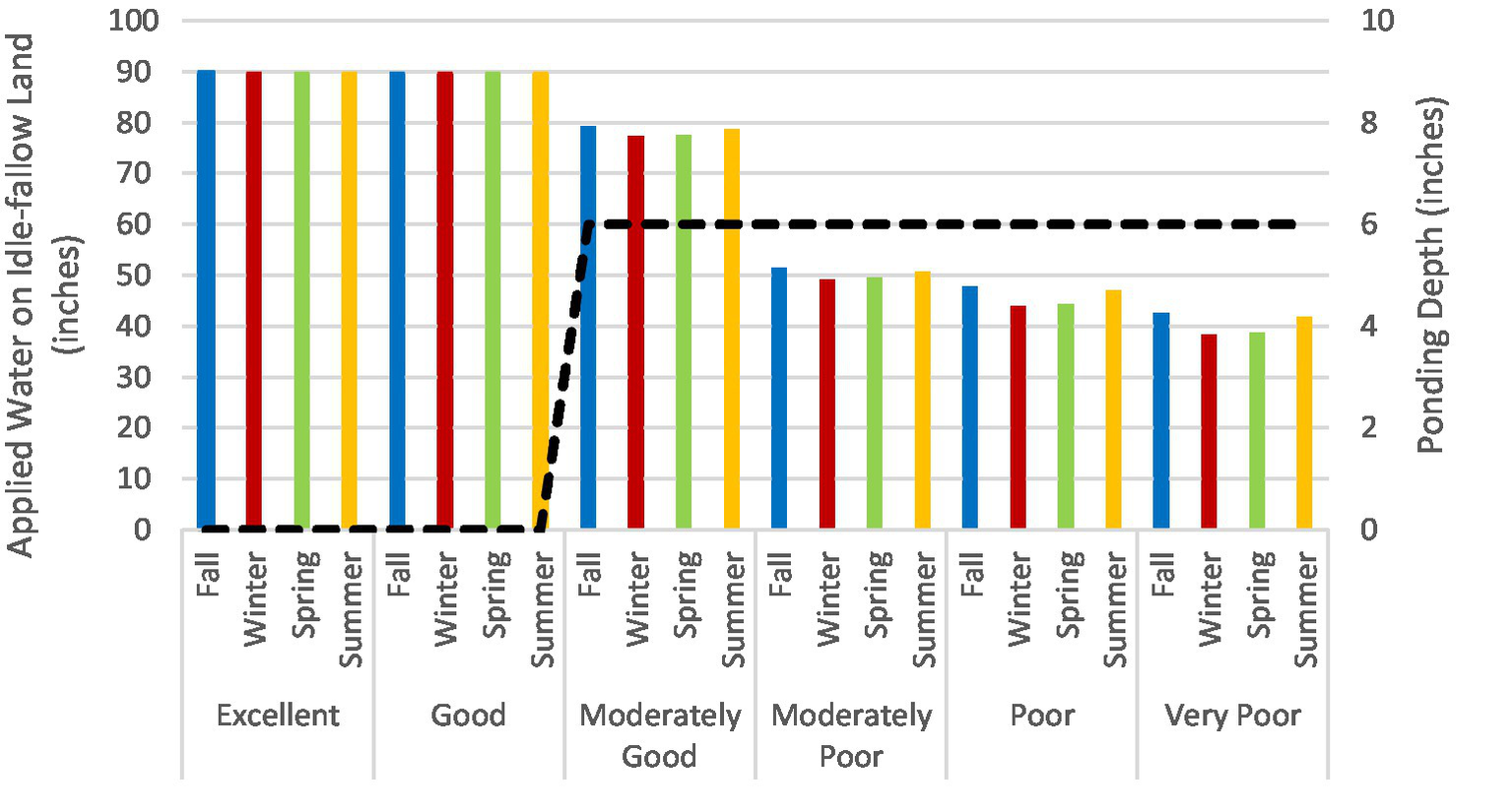
Applied water exclusively on Idle (fallow land) in all SAGBI soil types (primary Y-axis) and corresponding reached ponding depth (secondary Y-axis). Applied water delivery was 18 inches (45.72 cm) per day of water depth (15 cfs or 0.425 m3/s) over 5 consecutive days.
All conceptual IDC model results are used by the crop compatibility calendar in the Recharge Operation Model (Groundwater Recharge Assessment Tool (GRAT), 2025). CCC is a daily schedule that determines how many units of length (inches) of water can be safely applied to each soil-land use combination per day without reducing crop yields. The CCC adjusts the timing for application based on constraints of the crop life cycle (e.g., bloom, dormancy, etc.), field operation (e.g., pruning, timing of fertilizer application), and other practices that protect crop health and crop management. This daily recharge capacity is first filled with localized precipitation and then by the WAFR that is conveyed through irrigation districts’ conveyance, network and the field turnouts. In other words, the conceptual root-zone model does not consider precipitation in the mass balance calculations, however in the CCC, the daily applied water is reduced based on the daily observed precipitation.
4 Conclusion
In this manuscript, a conceptual root zone model is proposed to calculate the application amount and frequency of water available for recharge when Flood-MAR is implemented. The conceptual model uses physical soil parameters (e.g., hydraulic conductivity, saturation water content, field capacity, wilting point thresholds, effective porosity, and others) from Rawls et al. (1982), and the six top perennial crops (alfalfa, almonds, pasture, pistachios, vineyard, and walnuts) and fallow land in the San Joaquin Valley Watershed defined by the 2018 Land IQ database (California Department of Water Resources (CDWR), 2018a, 2018b).
The conceptual root zone model proposes to apply six inches (15.24 cm) of applied water on agricultural fields as a result of conveyance capacity and average acre field size. The results of the conceptual model were the amount of applied water, the reached saturation water content in the root zone not exceeding 75 percent saturation to avoid inhibiting plant respiration and growth, the potential return interval between applications for each soil-land use combination per day, and the amount of applied water needed to maintain six inches (15.24 cm) of ponding water depth in fallow land. All this information was used by the crop compatibility calendar in the recharge operation model to define daily schedules based on agricultural practices and biological constraints that ultimately determine how many units of length (inches) of water can be safely applied to each soil-land use combination per day without reducing crop yields.
The conceptual root zone model is a response to the need to develop a useful tool for water management in practice. It is important to acknowledge the limitations of this conceptual model. As it was shown, the model is a method that provides valuable information to guide water district managers and farmers when implementing Flood Managed Aquifer Recharge, works reasonably well, and might be useful for others. It is not a novel scientific finding, but the utility is outstanding. It is also acknowledged that there is a pragmatic need to develop a fuller assessment of the processes and limitations involved in calculating the application amount and frequency of water available for recharge.
Statements
Data availability statement
The original contributions presented in the study are included in the article/supplementary material, further inquiries can be directed to the corresponding author.
Author contributions
FF-L: Conceptualization, Formal analysis, Investigation, Methodology, Supervision, Visualization, Writing – original draft, Writing – review & editing. DA: Formal analysis, Funding acquisition, Methodology, Project administration, Resources, Writing – review & editing. MB: Data curation, Formal analysis, Writing – review & editing.
Funding
The author(s) declare that no financial support was received for the research and/or publication of this article.
Conflict of interest
The authors declare that the research was conducted in the absence of any commercial or financial relationships that could be construed as a potential conflict of interest.
Generative AI statement
The author(s) declare that no Gen AI was used in the creation of this manuscript.
Publisher’s note
All claims expressed in this article are solely those of the authors and do not necessarily represent those of their affiliated organizations, or those of the publisher, the editors and the reviewers. Any product that may be evaluated in this article, or claim that may be made by its manufacturer, is not guaranteed or endorsed by the publisher.
References
1
Abbott M. B. Bathurst J. C. Cunge J. A. O’Connel P. E. Rasmussen J. (1986a). An introduction to the European hydrological systems-systeme hydrologique Europeen, ‘SHE’. 1. History and philosophy of a physically based distributed modelling system. J. Hydrol.87, 45–59. doi: 10.1016/0022-1694(86)90114-9
2
Abbott M. B. Bathurst J. C. Cunge J. A. O’Connel P. E. Rasmussen J. (1986b). An introduction to the European hydrological systems-Systeme Hydrologique Europeen, ‘SHE’. 2. Structure of a physically based distributed modelling system. J. Hydrol.87, 61–77.
3
Arnold J. G. Kiniry J. R. Srinivasan R. Williams J. R. Haney E. B. Neitsch S. L. (2012). SWAT input/output documentation version 2012, vol. 654. Texas: Texas Water Resources Institute, 1–646.
4
Bachand S.M. Hossner R. Bachand P.A.M. . (2019). Effects on soil hydrology and salinity, and potential implications on soil oxygen, Bachand & Associates, final 2017 OFR Comprehensive Report: 38.
5
Balerdi C. Crane J. Schaffer B. (2003). Managing your tropical fruit grove under changing water table levels. EDIS. 2004.
6
Bali K. M. Mohamed A. Z. Begna S. Wang D. Putnam D. Dahlke H. E. et al . (2023). The use of HYDRUS-2D to simulate intermittent agricultural managed aquifer recharge (ag-MAR) in alfalfa in the San Joaquin valley. Agric. Water Manag.282:108296. doi: 10.1016/j.agwat.2023.108296
7
Brunner P. Simmons C. T. (2012). Hydrogeosphere: a fully integrated, physically based hydrological model. Groundwater50, 170–176. doi: 10.1111/j.1745-6584.2011.00882.x
8
California Department of Water Resources (CDWR) . (2015a). Integrated water flow model (IWFM-2015): theoretical documentation. Central Valley modeling unit, modeling support branch, Bay-Delta office, Sacramento. Available online at: http://baydeltaoffice.water.ca.gov/modeling/hydrology/IWFM/IWFM-2015/v2015_0_260/downloadables/IWFM-2015.0.260_TheoreticalDocumentation.pdf (Accessed December 01, 2023).
9
California Department of Water Resources (CDWR) (2015b) IWFM demand calculator (IDC-2015): theoretical documentation and user’s manual, Central Valley modeling unit, modeling support branch, Bay Delta office, Sacramento Available online at: http://baydeltaoffice.water.ca.gov/modeling/hydrology/IDC/IDC-2015/v2015_0_36/downloadables/IDC-2015.0.36_Documentation.pdf (Accessed December 01, 2023).
10
California Department of Water Resources (CDWR) . (2018a). Flood-MAR: Using flood water for managed aquifer recharge to support sustainable water resources. Available at: Department of Water Resources - Flood-Map White Paper June 2018
11
California Department of Water Resources (CDWR) . (2018b). 2018 statewide crop mapping GIS shapefiles (land IQ dataset). Available at: Statewide crop mapping - 2018 statewide crop mapping GIS shapefiles - California Natural Resources Agency open data
12
California Department of Water Resources (CDWR) . (2020). California water resilience portfolio. Available at: California Water Resilience Portfolio 2020.
13
California Department of Water Resources (CDWR) . (2022a). California’s water supply strategy. Available at: California's Water Supply Strategy Aug 2022.
14
California Department of Water Resources (CDWR) (2022b). Climate change vulnerabilities factsheet. Available online at: https://water.ca.gov/-/media/DWR-Website/Web-Pages/Programs/Delta-Conveyance/Public-Information/Climate-Change-Vulnerabilities_Factsheet_Dec22.pdf (Accessed December 01, 2024).
15
California Department of Water Resources (CDWR) . (2024). San Joaquin flood-MAR water studies. Study design. In preparation.
16
California Department of Water Resources (CDWR) . (2013). California simulation of evapotranspiration of applied water (Cal-SIMETAW). Available at: Agricultural Water Use Models.
17
Dahlke H. E. Brown A. Orloff S. Putnam D. H. O’Geen T. (2018). Managed winter flooding of alfalfa recharges groundwater with minimal crop damage. Calif. Agric.72, 65–75. doi: 10.3733/ca.2018a0001
18
Dogrul E. C. Kadir T. N. Chung F. I. (2011). Root zone moisture routing and water demand calculations in the context of integrated hydrology. J. Irrig. Drain. Eng.137:306. doi: 10.1061/(ASCE)IR.1943-4774.0000306
19
Ehtiat M. Jamshid Mousavi S. Srinivasan R. (2018). Groundwater modeling under variable operating conditions using SWAT, MODFLOW and MT3DMS: a catchment scale approach to water resources management. Water Resour. Manag.32, 1631–1649. doi: 10.1007/s11269-017-1895-z
20
Faunt C. C. Sneed M. Traum J. Brandt J. T. (2016). Water availability and land subsidence in the Central Valley, California, USA. Hydrogeol. J.24, 675–684. doi: 10.1007/s10040-015-1339-x
21
Ganot Y. Dahlke H. E. (2021). A model for estimating Ag-MAR flooding duration based on crop tolerance, root depth, and soil texture data. Agric. Water Manag.255:12. doi: 10.1016/j.agwat.2021.107031
22
Groundwater Recharge Assessment Tool (GRAT) . (2025). GRAT model documentation. In preparation.
23
Gyamfi C. Ndambuki J. Anornu G. (2017). Groundwater recharge modelling in a large scale basin: an example using the SWAT hydrologic model. Model. Earth Syst. Environ.3, 1361–1369. doi: 10.1007/s40808-017-0383-z
24
Harter T. (2015). California’s agricultural regions gear up to actively manage groundwater use and protection. Calif. Agric.69, 193–201. doi: 10.3733/ca.E.v069n03p193
25
Irrigation Training and Research Center (ITRC) . (2012).California polytechnic state university. Cal poly - ITRC
26
Levintal E. Kniffin M. L. Ganot Y. Marwaha N. Murphy N. P. Dahlke H. E. (2022). Agricultural managed aquifer recharge (ag-MAR)—a method for sustainable groundwater management: a review. Crit. Rev. Environ. Sci. Technol.53, 291–314. doi: 10.1080/10643389.2022.2050160
27
Liu Y. Wang A. Li B. Šimůnek J. Liao R. (2024). Combining mathematical models and machine learning algorithms to predict the future regional-scale actual transpiration by maize. Agric. Water Manag.303:9056. doi: 10.1016/j.agwat.2024.109056
28
Martinsen G. He X. Koch J. Guo W. Refsgaard J. Stisen S. (2022). Large-scale hydrological modeling in a multi-objective uncertainty framework – assessing the potential for managed aquifer recharge in the North China plain. J. Hydrol. Reg. Stud.41:1097. doi: 10.1016/j.ejrh.2022.101097
29
Neitsch S. L. Arnold J. G. Kiniry J. R. Williams J. R. (2011). Soil and water assessment tool: Theoretical documentation, version 2009. Texas water resources institute technical report no. 406. Texas, USA: Texas A&M University.
30
O’Geen A. Saal M. Dahlke H. Doll D. Elkins R. Fulton A. et al . (2015). Soil suitability index identifies potential areas for groundwater banking on agricultural lands. Calif. Agric.69, 75–84. doi: 10.3733/ca.v069n02p75
31
Orang M. Snyder R. L. Shu G. Hart Q. Sarreshteh S. Falk M. et al . (2013). California simulation of evapotranspiration of applied water and agricultural energy use in California. J. Integr. Agric.12, 1371–1388. doi: 10.1016/S2095-3119(13)60742-X
32
Rath S. Hinge G. (2024). Groundwater sustainability mapping for managed aquifer recharge in Dwarkeswar River basin: integration of watershed modeling, multi-criteria decision analysis, and constraint mapping. Groundw. Sustain. Dev.26:1279. doi: 10.1016/j.gsd.2024.101279
33
Rawls W. J. Brakensiek D. L. Miller N. (1982). Green-ampt infiltration parameters from soils data. Trans. ASAE25, 1316–1320. doi: 10.13031/2013.33720
34
Sallwey J. Glass Y. Stefan C. (2018). Utilizing unsaturated soil zone models for assessing managed aquifer recharge. Sustain. Water Resour. Manag.4, 383–397. doi: 10.1007/s40899-018-0214-z
35
SGMA (2025). Available online at: https://water.ca.gov/programs/groundwater-management/sgma-groundwater-management (Accessed December 01, 2024).
36
Šimůnek J. van Genuchten M. T. (2008). Modeling nonequilibrium flow and transport processes using HYDRUS. Vadose Zone J.7, 782–797. doi: 10.2136/vzj2007.0074
37
Šimůnek J. van Genuchten M. T. Šejna M. (2016). Recent developments and applications of the HYDRUS computer software packages. Vadose Zone J.15, 1–25. doi: 10.2136/vzj2016.04.0033
38
Yu J. Wu Y. Xu L. Peng J. Chen G. Shen X. et al . (2022). Evaluating the Hydrus-1D model optimized by remote sensing data for soil moisture simulations in the maize root zone. Remote Sens.14:6079. doi: 10.3390/rs14236079
39
Zhou T. Levintal E. Brunetti G. Jordan S. Harter T. Kisekka I. et al . (2023). Estimating the impact of vadose zone heterogeneity on agricultural managed aquifer recharge: a combined experimental and modeling study. Water Res.247:781. doi: 10.1016/j.watres.2023.120781
Summary
Keywords
floodwater for managed aquifer recharge, conceptual root zone model, water available for recharge, amount and frequency of WAFR, integrated demand calculator, integrated water flow model
Citation
Flores-López F, Arrate D and Bastani M (2025) A conceptual root zone model to calculate the application amount and frequency of water available for recharge. Front. Water 7:1554774. doi: 10.3389/frwa.2025.1554774
Received
02 January 2025
Accepted
26 May 2025
Published
18 June 2025
Volume
7 - 2025
Edited by
Josue Medellin-Azuara, University of California, Merced, United States
Reviewed by
Michael Tso, UK Centre for Ecology and Hydrology (UKCEH), United Kingdom
Mahesh Lal Maskey, Agricultural Research Service (USDA), United States
Updates
Copyright
© 2025 Flores-López, Arrate and Bastani.
This is an open-access article distributed under the terms of the Creative Commons Attribution License (CC BY). The use, distribution or reproduction in other forums is permitted, provided the original author(s) and the copyright owner(s) are credited and that the original publication in this journal is cited, in accordance with accepted academic practice. No use, distribution or reproduction is permitted which does not comply with these terms.
*Correspondence: Francisco Flores-López, francisco.floreslopez@water.ca.gov
Disclaimer
All claims expressed in this article are solely those of the authors and do not necessarily represent those of their affiliated organizations, or those of the publisher, the editors and the reviewers. Any product that may be evaluated in this article or claim that may be made by its manufacturer is not guaranteed or endorsed by the publisher.