Passively heated fiber optic distributed temperature sensing for long-term soil moisture observations

This paper presents a strategy to improve spatial and temporal volumetric water content (VWC) using passive DTS observation. We demonstrate this method using 22 months of passive fiber optic distributed temperature (FO-DTS). This method has previously encountered challenges, primarily due to noise effects and instability of diurnal temperature. We improve the water traceability by employing numerical estimation of the soil thermal diffusivity. This method was tested on a slope catena at the Draix–Bléone Mediterranean catchment (South-East France) and with synthetic data prior to applying it to field-scale scenarios. The results show a good performance as indicated by a determination coefficient of 0.92, a root mean square error of 0.06 m³/m³ and a mean relative percentage error of 1.41%. We conclude that the proposed strategy is convenient for analyzing passive DTS experiments using diurnal heat sources, where reliable thermal diffusivity and VWC data can be obtained without the use of active application sources.

1 Introduction

Numerous techniques have been devised to monitor space and time variations of soil-water content, including direct manual soil sampling, and indirect methods using electromagnetic, thermophysical and radiation-based instruments. The direct manual technique of soil sampling and further gravimetric weighting can be considered as the reference method, but it is limited by the spatial representativity of the samples. Consequently, indirect methods emerged as promising approaches for wide areas survey and long-term continuous monitoring. Various active and passive radiation instruments, including neutron probes, cosmic-ray neutron sensors (CRNS), electromagnetic sensors, and thermophysical-based methods, have been widely applied as indirect techniques for soil moisture measurement. Neutron probes, for instance, remain a reliable method for measuring soil moisture due to their ability to penetrate deeply into the soil profile and deliver high accuracy (Zhang, 2017). Cosmic-Ray Neutron Sensors (CRNS) have also emerged as a promising noninvasive technique for field-scale soil moisture estimation, capable of covering large areas with minimal calibration requirements (Stevanato et al., 2019). Electromagnetic sensors, particularly Time Domain Reflectometry (TDR) and Frequency Domain Reflectometry (FDR), continue to be widely used due to their precision and adaptability to a wide range of soil types (Zhu et al., 2019). In addition, recent advances in thermophysical-based sensors—which estimate soil moisture through analysis of soil thermal properties—offer novel opportunities for application in precision agriculture and distributed sensing. Hybrid sensing methods combining soil permittivity and temperature have also been proposed (Chavanne and Jean-Pierre, 2014).

Soil temperature is a readily measurable environmental parameter that enables the derivation of volumetric water content (Béhaegel et al., 2007). Fiber Optic Distributed Temperature Sensing (FO-DTS) has been employed as a primary method for soil temperature measurements (Bense et al., 2016) and indirect estimations of soil moisture using active and passive measurements (Dong et al., 2017; Steele-Dunne et al., 2010). In practice, FO-TDS can measure a lot of temperature data from optical fibers embedded in shallow soil and on the ground surface with a vertical grid configuration. FO-DTS temperature measurements rely primarily on inelastic light scattering mechanisms, particularly Raman and Brillouin scattering. Raman scattering, especially the anti-Stokes component, is commonly used in FO-DTS systems due to its high sensitivity to temperature, enabling temperature resolution as acceptable as ±0.01°C under controlled conditions. In contrast, Brillouin scattering is often employed in systems designed for simultaneous temperature and strain measurements (Hartog et al., 2019; Selker et al., 2006). In this study, we chose Raman-based FO-DTS because it provides a direct and reliable relationship between the backscattered signal and temperature, without the need for strain compensation. This makes it particularly well-suited for soil applications where mechanical disturbances and strain effects are minimal or not of primary interest. Brillouin scattering is typically used in systems that require simultaneous temperature and strain measurement (Smith et al., 1999; Zhou et al., 2013), which was not the focus of our work. In addition, Rayleigh scattering also occurs in optical fibers, but it is generally not relevant for temperature measurement because it lacks sufficient thermal sensitivity (Loranger et al., 2015; Palmieri, 2014). Instead, Rayleigh-based methods are more commonly applied in distributed acoustic sensing (DAS) and high-resolution strain detection systems (Shang et al., 2022).

In active FO-DTS mode, an active thermal source is created by a heat source, maintained for a few seconds to minutes, and influences a shielded cable via the Joule effect (Ciocca et al., 2012; Sayde et al., 2010). Analyzing the temperature decay with time allows the volumetric water content (VWC) of a soil to be determined with an error of <7% (Cao et al., 2015; Weiss, 2003). The accuracy of the active mode measurements exhibits a first-order proportional relationship with the water content. When the volumetric moisture content is 0.05 m³m⁻³, the standard deviation of the readings is 0.001 m³m⁻³, whereas, at a volumetric moisture content of 0.41 m³m⁻³, the standard deviation is 0.046 m³m⁻³ (Sayde et al., 2010). The main drawback of active FO-DTS is that an external power source is required to generate the thermal source, which is complex to setup in remote areas and for long-term measurements.

In the passive measurement of VWC FO-DTS mode, the thermal source is created by the surface energy flux. Temporal variations in energy follows a diurnal period independent of local and global weather changes and shifts in vegetation cover (Sigmund et al., 2017). Several strategies for tracing soil VWC using passive temperature observations were developed (Halloran et al., 2016) using local measurements (e.g., point probe sensors) either installed on vertical profiles (Bechkit et al., 2014) or placed along cross-sections (Anderson, 2005).

For soil VWC estimations based on thermophysical properties, passive FO-DTS is simpler but less accurate than active heated DTS (Ciocca et al., 2012; Steele-Dunne et al., 2010; Striegl and Loheide, 2012; Suárez et al., 2011). Indeed, using natural heat fluxes as a thermal source requires the characterization of radiative, convective and conductive components; such measurements are rarely achievable in the field. Consequently, estimating soil VWC using this mode is sensitive to many factors (Cao et al., 2015), including air temperature differences, vegetation cover, seasons and weather condition. The first approach for estimating volumetric water content (VWC) involves data assimilation, which utilizes temperature measurements to determine VWC. This method enhances accuracy by incorporating empirical correlations between temperature and soil moisture in shallow soil layers (i.e., the top ∼50 cm) (Dong et al., 2015). The second approach estimates soil VWC by calculating thermal diffusivity through solving the heat transfer equation. de Jong van Lier and Durigon (2013) proposed a method to calculate soil thermal diffusivity based on temperature measurements at multiple depths. This analytical approach analyzes the amplitude damping and phase lag between temperature measurements (de Jong van Lier and Durigon, 2013). This approach is strongly dependent on the sinusoidal waveform of soil temperature, which varies on diurnal, seasonal and annual periods (Carslaw and Jaeger, 1959; de Jong van Lier and Durigon, 2013). Therefore, diffusivity estimated from time-resolved techniques can be used to infer spatially distributed daily average VWC values along the sensing domain. Another study described vertical water flows by calculating thermal diffusivity using a simple numerical finite element scheme based on soil temperature profiles (Tabbagh et al., 2017). This approach allows the thermal properties of a soil to be determined over short distances and at any desired time interval (Tabbagh et al., 2017). The same approach was used by Krzeminska et al. (2012) to apply an explicit finite difference scheme to track the spatial variability of soil–water saturation in an area influenced by landslides (Krzeminska et al., 2012). The method is dependent on the inversion and the choice of the duration of the optimization window. While these studies demonstrate the potential of temperature-based models, they are often limited to short-term observations or specific slope conditions. They typically require intensive data inversion or calibration schemes, which may not be feasible for long-term, distributed field deployments. To address these limitations, our study focuses on developing a passive heating FO-DTS strategy to monitor volumetric water content (VWC) over extended periods and across heterogeneous soil conditions, using thermal response data. We aim to explore the feasibility of this approach for characterizing soil moisture dynamics in a field setting.

In this context, we consider the Draix–Bléone catena area, namely the Laval-Moulin divide, characterized by unsaturated marly slopes influenced by Mediterranean climatic conditions (Mathys et al., 2005). This area features slope surface erosion (gullying, shallow landslides slides) and sediment transport and has been extensively studied since 1983 (Mathys et al., 2005). Documenting soil–water content changes at the scale of a catena or larger hydrological units typically requires the deployment of invasive local sensors (e.g., TDR, FDR, neutron probes), which can be costly and physically disrupt the soil structure and hydrological connectivity of the monitored site (Bogena et al., 2007). Hence, we used FO-DTS (Steele-Dunne et al., 2010) to monitor water content based on temperature measurements (Rutten et al., 2010) at high frequency and spatial resolution (Seyfried et al., 2016). For long-term and continuous observations, passive FO-DTS provides simpler measurement opportunities. This is different with active FO-DTS, where it requires a lot of resources to produce active heating. This need creates difficulties for measurements in the field where there is no power and shelter available.

In response to these challenges, this study explores using fiber-optic distributed temperature sensing (FO-DTS) as a minimally invasive alternative for monitoring soil–water content at high spatial and temporal resolutions. Specifically, we aim to evaluate the feasibility of using passive FO-DTS for long-term soil moisture observation under field conditions where active heating and continuous power supply are impractical. To address this objective, we propose a hybrid approach that combines signal processing and numerical modeling to estimate soil volumetric water content (VWC) from temperature data collected along a 60-meter soil catena. FO-DTS provides direct soil temperature measurements along the fiber optic cable, while VWC is derived from these temperature data through thermal modeling and inversion methods. The spatial resolutions applied in this study, 5 cm vertically and 50 cm horizontally, were selected based on the achievable spatial sampling density of the DTS configuration and the need to capture meaningful soil moisture variability across the hillslope scale. The specific aims of this study are as follows: (i) to estimate volumetric water content with a vertical resolution of 5 cm and a horizontal resolution of 50 cm along the transect; and (ii) to describe and analyze long-term volumetric water content variations over a 22-month monitoring period, based on measurements collected at 6-min intervals.

2 Materials and methods

2.1 The Draix–Bléone (South-East France) hydrological research catchment

The observation site is the Draix–Bléone catchment, which features many watersheds and catenas, and is representative of landscapes in the Southeast French Alps (Antoine et al., 1995; Mathys et al., 2005). The investigated catena is the Laval-Moulin divide, located on the divide separating the Moulin stream to the West and Laval stream to the East (Figure 1a). The catena is composed of altered regolith comprising Callovo-Oxfordian black marls with a clay shale facies (Marc et al., 2017a). The catena is partly covered by grass and Pinus Negra trees with a vegetation density up to 45% (Mathys et al., 2003). Frequent freeze and thaw cycles in winter influence the weathering of the black marls and thus the soil properties.

Figure 1

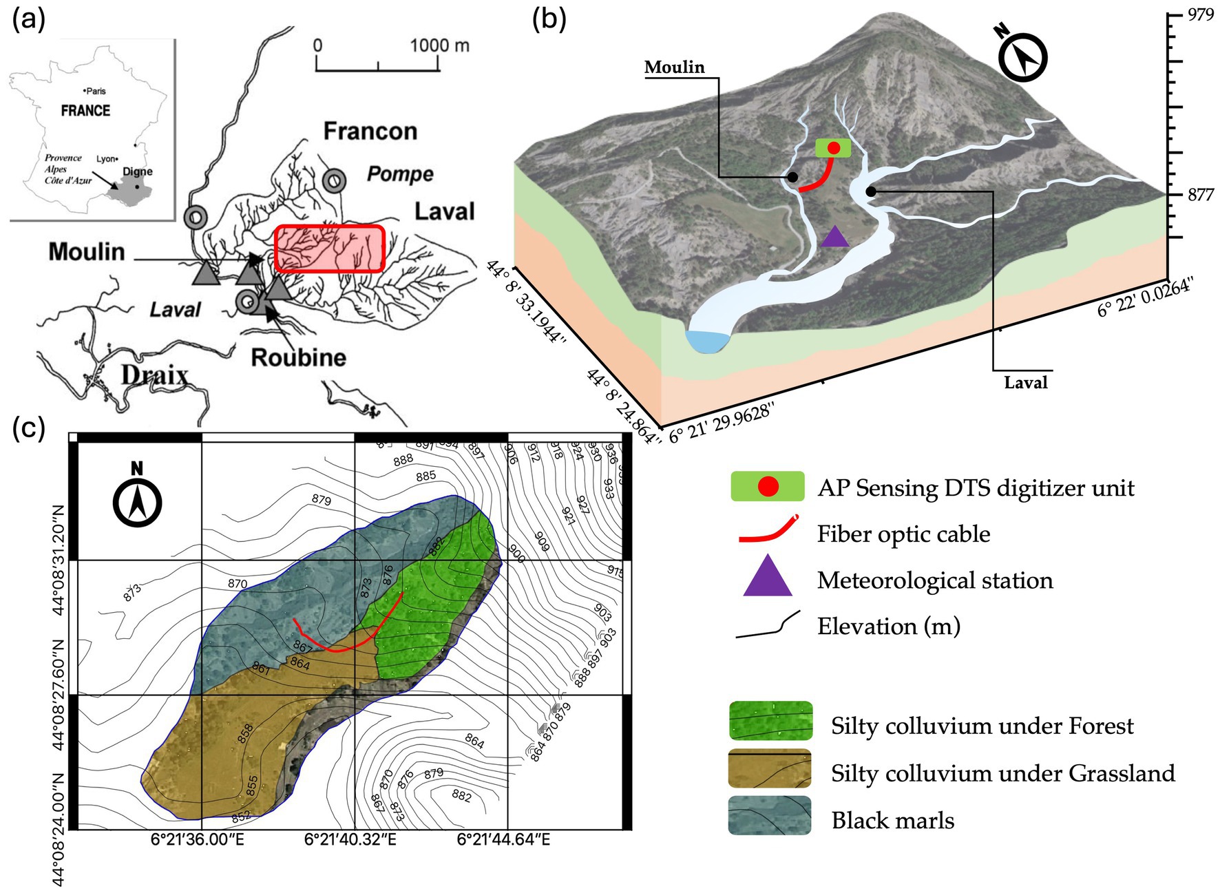
Figure 1. Draix–Bléone catchment hydrological research observatory. (a) Location of the investigated divide between the Moulin and Laval catchments (Mathys et al., 2005). (b) 3D view of the study site and position of the measuring instruments. (c) Soil map of the divide with colluvium soil under forest (green), colluvium soil under grass (brown), and weathered black marls (blue).

The Draix–Bléone catchment has a Mediterranean climate with an annual rainfall of 900 mm (Mathys et al., 2003). The area has on average 200 days a year without rain, 160 days with <30 mm rainfall and only 5 days with more than 30 mm rainfall. The mean annual potential evapotranspiration is 650 mm (Esteves et al., 2005). Summers are dry with occasional storms and the maximum precipitation and runoff occur in spring and autumn.

We investigated a 60 m catena crossing three soil units, consisting of argillaceous weathered black marls, silty colluvium with grassland, and silty colluvium under forest. The catena faces South (Figure 1a), with the weathered black marls soil unit at the West and the silty colluvium unit at the East (Figures 1b,c). Below the study site, the superficial formations vary considerably in thickness, texture (and thus porosity), compactness, organic matter content, and VWC depending on local structural, topographic and vegetation conditions (Maquaire et al., 2002). A total of 84 soil samples were collected to characterize the vertical and horizontal variability of soil properties. Sampling was conducted at four depths, such as 5, 10, 15, and 30 cm, with 21 samples obtained per depth. These samples were evenly collected across three representative soil conditions: black marl, soil under grass, and soil under forest, resulting in 7 samples per soil type at each depth. No samples were collected from the soil surface (0–5 cm), as this layer is often directly exposed to atmospheric dynamics and thus considered less stable and more prone to disturbance, which may not accurately represent the underlying soil characteristics. The samples were collected using augers and metal cylinders to minimize disturbance and preserve the natural soil structure. All samples were analyzed in the CNRS/EOST Soil Laboratory (LAS) using a CoulterLS particle size analyzer to determine grain size distribution and to support the assessment of physical soil properties. Furthermore, the saturated hydraulic conductivity was estimated using the constant head method, while the retention pF curves were determined using the van Genuchten model (van Genuchten, 1978).

2.2 The FO-DTS experimental setup at the Moulin-Laval divide

As illustrated in Figure 2a, a 350 m long reinforced fiber optic cable was horizontally buried across three distinct soil types at 0 cm (ground level), −5 cm, −10 cm, and −15 cm, along a 60-meter transect. Soil temperature was measured using a FO-DTS digitizer from Advanced Photonic Sensing (AP Sensing) equipped with a Brugg Fiber Optic cable manufactured by Brugg Cable AG in Switzerland. The fiber optic is protected by Polyamide Nylon PA12 outer sheath for outdoors harsh environments application (BRUsens Temperature LLK-BSTE 150°C 3.8 mm). The sensing cable was installed by carefully incising the soil over 20 cm (Figures 2b,c), thereby minimizing soil disturbance, and the vertical interlace of 5 cm was controlled using a specific mechanical template.

Figure 2

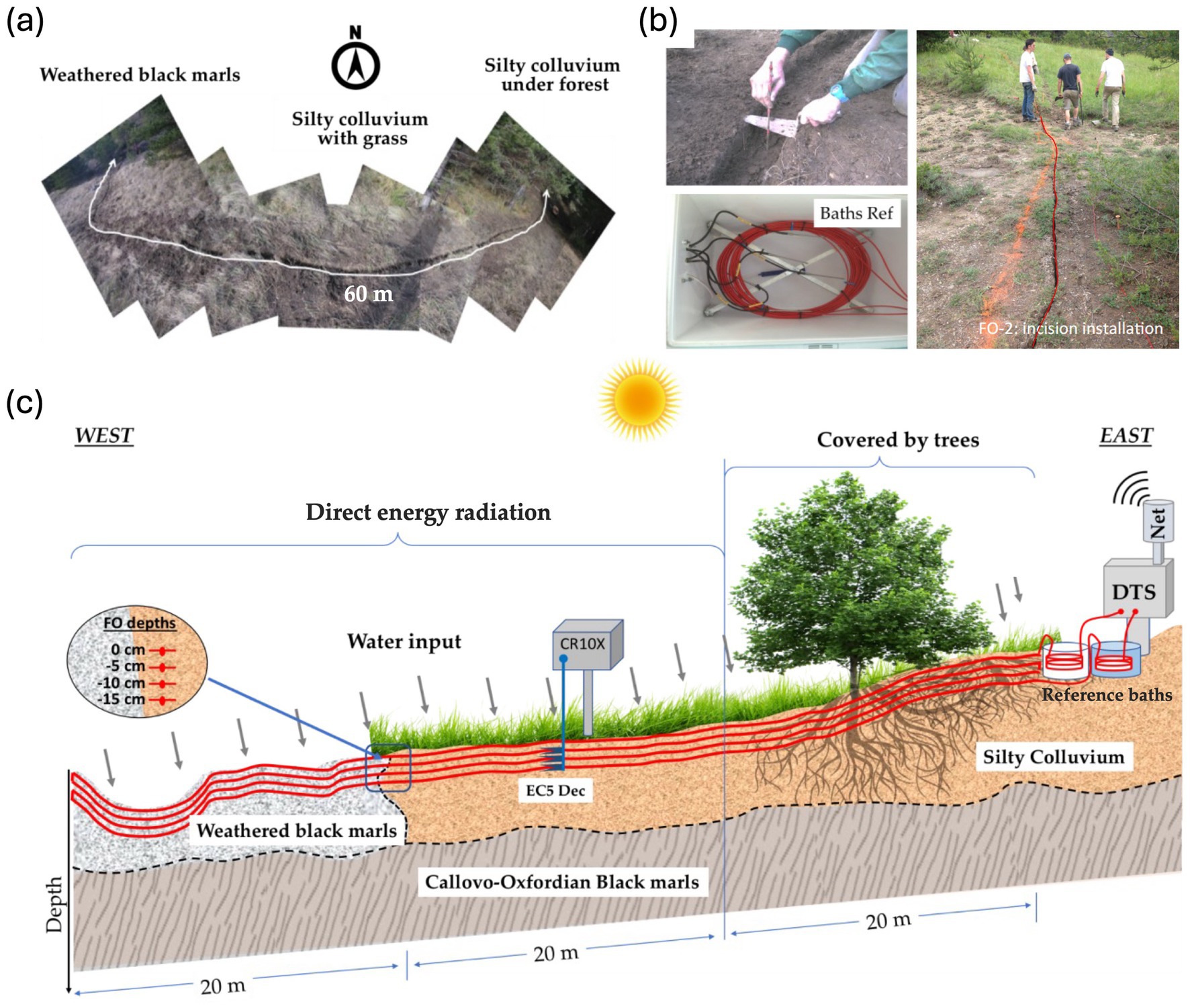
Figure 2. The Draix-Bléone FO-DTS instrumental setup: (a) Aerial photograph describing the fiber optic cable installation crossing the three soil types horizontally. (b) Fiber optic cable installation at the start of the experiment. (c) Schematic diagram of the network of instruments (FO-DTS, reference baths, point-based Decagon EC5 soil moisture probe sensors for validation at depths of −5, −10 and −15 cm, respectively).

The AP Sensing digitizer has a power consumption of approximately 17 Watt at 20°C ambient temperature (10–30 VDC). The internal memory provides 16 GB of storage space, and the LAN port connecting the digitizer to the remote network. Binary file formats are used to minimize the temperature trace file size. Hence, the digitizer can monitor temperature profiles for up to 24 months. The FO-DTS digitizer provides a raw temperature reading calibrated to the internal calibration coil; however, its internal calibration is based on default assumptions, such as connector losses, attenuation of the fiber, and environmental sensing considerations with time-varying errors that typically exceed 1 K (van de Giesen et al., 2012).

Soil temperature was measured every 6 min at a spatial resolution of 0.50 m using a double-ended cable configuration to obtain higher accuracy temperature measurements. In this configuration, the decay of photons along the length of the sensing cable (attenuation along the fiber optic and effect of splices, effect of fiber optic heterogeneities) was compensated by loops of fiber optic cable in two reference baths filled with 10 liters of water at the start and end of the profile (Figure 2c). There are two baths with different temperatures, and we tried to always have a difference of about 20° C between each bath. The first is a bath with the ambient water temperature; this ambient reference bath is equipped with five PT100 independent temperature probe sensors and the water is mixed (to avoid layering) with a small pump. The second is a bath with a controlled water temperature called “warm reference bath.” This warm reference bath is equipped with a heater (used for aquariums), five PT100 independent temperature probe sensors, and a pump to mix the water in the bath. Water temperature data on the ambient and heated baths were logged using a Campbell CR1000 datalogger. The mean and standard deviation values of water temperature in the baths were used to correct the fiber optic cable temperature according to the method proposed by van de Giesen et al. (2012).

The slope catena is further instrumented with three capacitance-based soil moisture probes (EC-5 Decagon) located at 30 m distances along the fiber optic cable and buried at depths of −5, −10 and −15 cm (Figure 2c). A meteorological station equipped with a tipping bucket ARG100 rain gauge, a CS300 pyranometer, a CS300 anemometer and a CS215 air temperature and relative humidity probe were positioned downhill of the FO cable at a distance of 140 m. All variables were acquired at a sampling period of 10 min. The method proposed by Sigmund et al. (2017) was used to correct the effect of radiation on the temperatures measured by the FO cable at the slope surface (Sigmund et al., 2017).

2.3 Methods

The concept addressed in this paper combines signal processing and soil temperature numerical temperature using the heat equation in order to reveals variations of soil moisture. Soil thermal properties, such as saturated and dry heat conductivities and volumetric heat capacity, must be estimated; however, soil thermal diffusivity depends on soil moisture and both above depend on rainfall events.

Figure 3 describes the data processing workflow. The workflow consists of soil temperature data acquisition, calibration and correction, determination of soil thermal properties using numerical calculation and signal processing, and non-linear inversion of soil thermal parameters. The first step is data acquisition of the soil temperature using FO-DTS (Raw T^o FO-DTS). The second step is the calibration and correction procedures. This procedure is necessary to correct the Raw T^o from attenuation losses in the fiber optics cable and the influence of air solar radiation on the cable at the soil surface (see Figure 2c). The third step is the determination of soil thermal diffusivity (D) using a numerical approach and applying time-series signal processing to reduce known disturbances, such as diurnal and annual variations of apparent diffusivity (D_app). Apparent soil thermal diffusivity was calculated using the vertical temperature profile during periods of observation between January 2016 and April 2018. A one-dimensional temperature profile consideration was used to simplify the determination of soil thermal diffusivity. The fourth step is a nonlinear inversion to retrieve the soil thermal parameters and VWC calculation. The soil thermal parameters include heat conductivity (λ_s and λ_d), heat capacity (C_s), and true soil thermal diffusivity (D). The Johansen model is used for VWC calculation. According to the constitutive workflow shown in Figure 3, the calculated VWC is compared with the direct measurements from EC-5 probes. The optimized soil parameters are inferred by inversion of the van Genuchten model, the input variable being the measured VWC. Error analysis is used to quantify the accuracy of the calculation.

Figure 3

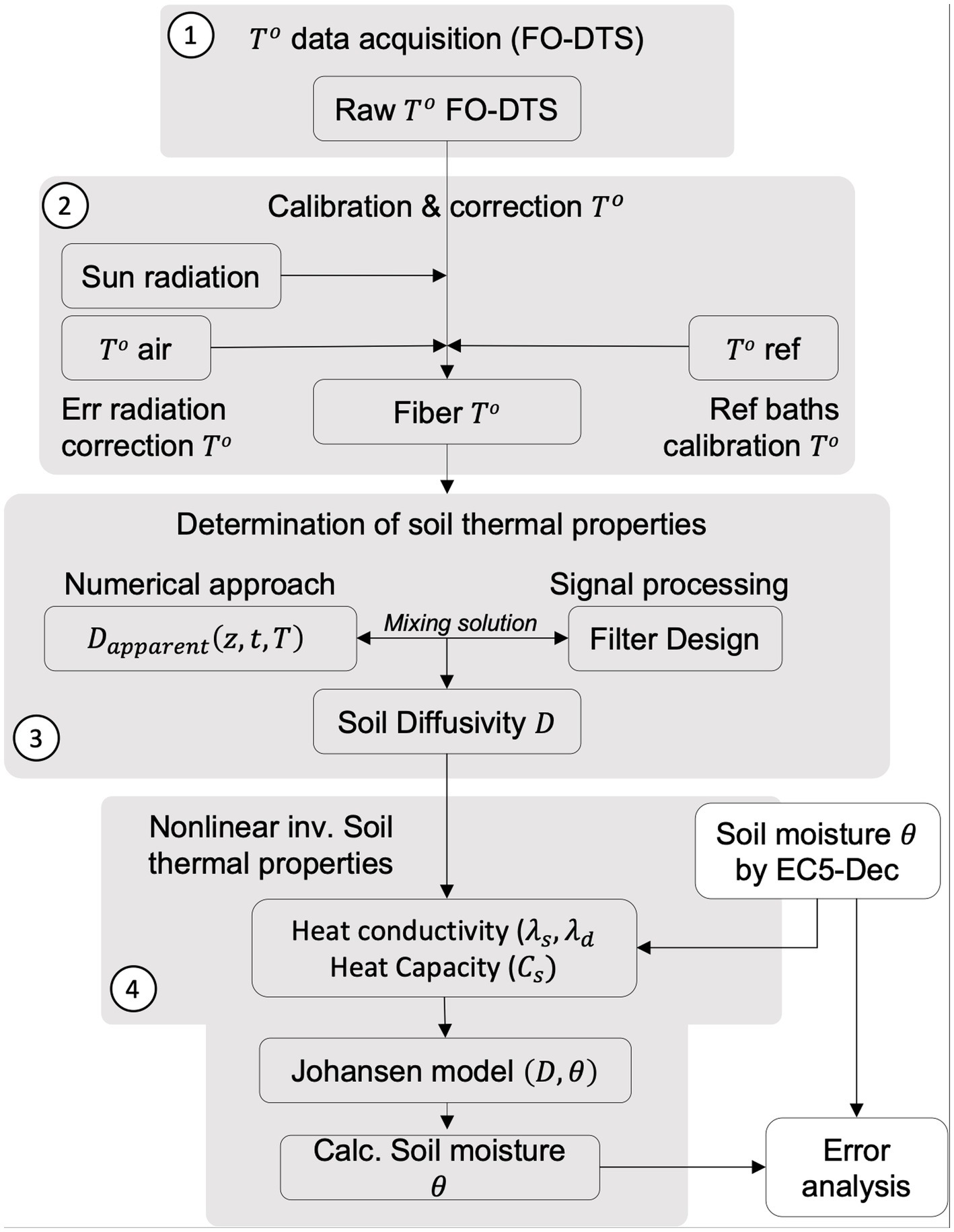
Figure 3. Workflow of the hybrid solution mixing soil temperature numerical modeling and signal processing to estimate soil VWC from passive FO-DTS time series.

2.4 Calibration and correction of T^o

Long-term and dynamic calibration of FO-DTS systems is essential for maintaining measurement accuracy over extended deployments, especially in variable environmental conditions. Several studies have addressed this need by proposing site-specific, time-varying calibration approaches that account for changes in ambient temperature, instrument drift, and cable degradation. Dynamic calibration emphasized the importance of applying repeated reference section calibration and dual-ended configurations to correct for temporal and spatial drift (Liu et al., 2023; Lu et al., 2023; McDaniel et al., 2016, 2018).

In our experiment, the optical fiber cable is deployed on the ground using a double-ended configuration and is crossing ambient and warm reference baths, which enables inherent correction for differential attenuation along the fiber and improves the spatial consistency of temperature measurements (see Figure 2c). This configuration allows temperature calibration along the cable with reference to 10 independent temperature sensors (PT107) spread in the two reference baths. Temperature readings along the fiber contain the dynamic calibration parameter C (t) (van de Giesen et al., 2012). The values of C (t) temperatures are linked to independent temperature readings measured by the PT107 sensors at several positions. We assume that C (t) is a function of the linear reading of the temperature. Thus, the fiber optic temperature reading is calibrated by the C (t) values. By integrating a double-ended approach with periodic referencing and stability checks, our system balances accuracy with practical field operability, making it suitable for extended soil moisture monitoring under low-maintenance conditions.

While the buried fiber optic cable measures the soil temperature, the unburied fiber cable at the soil surface measures the temperature at the interface between the ground and the air. This configuration allows the fiber to receive heat directly from solar radiation, thus influencing soil temperature readings at the surface. This effect is corrected by subtracting the fiber optic temperatures on the topsoil with an energy balance model including the short and long-wave convective and conductive heat transfer processes (Sigmund et al., 2017). The basic principle of this method is to use the shortwave, longwave, convective, and conductive heat transfer around the fiber for quantifying the modeled radiation. In our application, we use the CS300 pyranometer produced by Campbell Scientific for providing total wave irradiance datasets that are installed at the meteorological station (see Figure 1). In addition, we used PT100 to measure the air temperature around the fiber and installed it at 1.7 m above the soil. In this case, the fiber cable located in the surface layer is 60 m it is possible to have an aerial error reading. The albedo and emissivity remained constant and referred to the fabric’s datasheet that varied maximum ± 20% and −12 to +33% for albedo and emissivity, respectively. This correction consists of incoming energy flux from the conduction of fiber cable and outgoing convective energy exchange with moving air, shortwave, and longwave radiation.

2.5 Determination of soil thermal properties

Heat transfer in relation to water content below the surface has been widely studied (Cheviron et al., 2005; Rutten et al., 2010). Estimating water content, using thermal properties as a proxy, can be performed with the heat transfer equation (Halloran et al., 2016). Vertical heat transfer describing subsurface heat flux density in soil is controlled by both conductivity and volumetric heat capacity, which are functions of water content and soil porosity (Adeniyi and Oshunsanya, 2012). The relationship between heat conductivity and heat capacity is described as soil thermal diffusivity while the combination of vertical heat transport and heat conservation can be simplified as the diffusion equation (Equations 1, 2):

$\begin{array}{ll}\frac{\partial T}{\partial t}=\frac{\lambda \left(\theta \right)}{C\left(\theta \right)}\frac{{\partial }^{2}T}{\partial z^2}& (1)\end{array}$

$\begin{array}{ll}\frac{\partial T}{\partial t}=D\left(\theta \right)\frac{{\partial }^{2}T}{\partial z^2}& (2)\end{array}$

Where C (J m⁻³ K⁻¹) is the volumetric heat capacity of soil, λ (W m⁻¹ K⁻¹) is soil heat conductivity, D (m² s⁻¹) is soil thermal diffusivity which is ratio of λ/C, and all thermal parameters are functions of water content $\left(\theta \right)$ . T (K) is soil temperature, z (m) is the depth of the soil column, and t (s) is time. In accordance with Equations 1, 2, conduction is assumed to be the dominant mode by which heat transfer occurs in the subsurface; other heat transfer modes are neglected due to their relatively low contribution to temperature dynamics (Krzeminska et al., 2012; Rutten et al., 2010; Van Wijk and Derksen, 1966). Further, subsurface vapor flows are ignored because they occur rarely in the dry seasons (Chung and Horton, 1987). Therefore, we assumed that water vapor transport was purely diffusive, and that convection was negligible. At least six methods have been developed to determine the apparent thermal diffusivity of near-surface soil (Horton et al., 1983). One of these methods involves numerical discretization applied with the explicit finite difference to solve Equation 2. This method allows thermal diffusivity to be estimated from three temperature measurement depths.

Below the surface, temperature variations follow the average temperature during one cycle and the temperature amplitude at the ground surface. In addition, rainfall events influence subsurface temperatures and temperature propagation due to water content. Considering that heat transfer is determined by the damping depth factor, which itself depends on the thermal diffusivity and temperature period of soil (Krarti et al., 1995; Wu and Nofziger, 1999), temperature behavior can be predicted using Equations 1, 2 involving boundary conditions and damping depth (Cichota et al., 2004; Oyewole et al., 2018). Hence, the solution of the heat equation satisfying boundary condition is given with Equation 3 (Carslaw and Jaeger, 1959):

$\begin{array}{ll}T(z,t)=T_0+A_0{e}^{\left(\frac{-z}{d}\right)}sin(\frac{2\mathit{\pi t}}{\tau }-\frac{z}{d})& (3)\end{array}$

where T₀ is the average temperature during one cycle, A₀ is the temperature amplitude at the soil surface, d is the damping depth factor with $d=\sqrt{\mathit{\tau D}/\pi }$ , τ is the diurnal period (in second), z is the depth (in centimeter), and t is time (in second). The apparent thermal diffusivity from the damping depth factor in Equation 3 is calculated using analytical and numerical solutions. Apparent soil thermal diffusivity is obtained by selecting the value of soil thermal diffusivity to minimize the sum of temperature square differences between the model and observations (Horton et al., 1983). Horton et al. (1983) showed in his experiment that the apparent thermal diffusivity of soil over three days is approximately 5.7 × 10^-7 to 6.2 × 10^-7 m²s⁻¹ with a standard deviation of <4.4 × 10^-7 m²s⁻¹ at a depth of −5 cm; however, this approach only allow estimating a daily single apparent diffusivity.

In our approach, soil thermal diffusivity is calculated every 6 min. Theoretically, we could detect thermal diffusivity and, therefore, water content change between two estimations with a 6-min resolution. In practice, the real resolution on the thermal diffusivity and on water content is higher and variable because it depends on the frequency content in the input temperature signal and on the thermal diffusivity value itself. From our dataset, we estimate the minimal resolution to be around 12 h. Therefore, this is one of the limitations of this method in its application. On the one hand, diurnal temperature waveforms in the passive heat source application can result in minor temperature differences between the upper and lower boundaries. These situations yield overestimated soil diffusivities in the morning and evening when the upper boundary temperature encounters increasing or decreasing temperatures. This overestimation was mentioned by Krzeminska et al. (2012) because the temperature signal was assumed to be a sinusoidal function. This frequently overestimated soil thermal diffusivity is considered an “artifact” because it appears repeatedly. Hence, the estimated soil thermal diffusivity in the time domain contains not only the water content effect but also diurnal and annual variations due to the temperature sinusoidal waveform (Equation 4).

$\begin{array}{ll}D\left(t\right)=D_{\mathit{wc}}\left(t\right)+D_{\mathit{\text{diurnal}}}\left(t\right)+D_{\mathit{\text{annual}}}\left(t\right)& (4)\end{array}$

Where D(t) is the calculated soil thermal diffusivity in the time domain, consisting of the response of water content variation (D_wc) and the artifact, namely the apparent soil thermal diffusivity due to diurnal (D_diurnal) and annual (D_annual) fluctuations. The apparent soil thermal diffusivity response generally experiences an extreme increase at sunrise and sunset. On the other hand, the thermal diffusivity also increases due to the presence of water content. This response is found in both analytical and numerical soil thermal diffusivity calculations on passive DTS optic setups. This artifact associated with diurnal temperature heat sources can be investigated using spectrum analysis. The Fast Fourier Transform (FFT) shown in Equation 5 presents periodically overestimated soil thermal diffusivity in the frequency domain such that the artifact can be removed using a specific filter design.

$\begin{array}{ll}D\left(\omega \right)={\int }_{-\infty }^{\infty }D\left(t\right)e^{-\mathit{j\omega t}}\partial t& (5)\end{array}$

The aperiodic signal due to water infiltration and drainage is expected to pass as a filtering result. The filter is also expected to remove noise from the measurement uncertainty or temperature fluctuation due to wind flow, cloudy weather, or any other factors provoking different soil temperature over short time periods. The Butterworth band-stop filter is used for removing these signals with the selection of an appropriate cutoff frequency tailored to our application. The filtered value of soil thermal diffusivity may be impacted by noise reduction during signal filtering, but the filtered soil thermal diffusivity remains in agreement with water content changes with time. To anticipate the biased VWC from the filtered soil thermal diffusivity, we converted filtered soil thermal diffusivity into relative saturation.

2.6 Inversion of soil thermal parameters and VWC calculation

The inversion of soil thermal diffusivity to relative saturation in the Johansen model (Equation 6) presents a constitutive relationship of the dependency of thermal diffusivity to water content. In terms of soil thermal diffusivity calculations, a nonlinear relation exists between water content (θ) and soil thermal diffusivity [D(θ)] as follows:

$\begin{array}{ll}D\left(\theta \right)=\frac{K_e({\lambda }_s-{\lambda }_d)+{\lambda }_d}{(1-\varnothing )C_s+{\mathit{\theta C}}_w}& (6)\end{array}$

Where θ is relative saturation of volumetric water content, ɸ is soil porosity, ${\lambda }_d$ and ${\lambda }_s$ are dry and saturated heat conductivity (W m⁻¹ K⁻¹), respectively, and $C_s$ (J m⁻³ K⁻¹) is soil matrix heat capacity. The formula in Equation 6 provides physical thermal coefficients that are within the heat property ratio of the soil heat conductivity and capacity. Soil heat conductivity is a linear combination of saturated and dry heat conductivities. The Kersten number (Kersten, 1949) for unfrozen fine soil is then used to determine the normalized soil heat conductivity in dry and saturated soil (Béhaegel et al., 2007). Kersten number is expressed by $K_e={log}_{10}\left(\frac{\theta }{\varnothing }\right)+1$ .

Estimating soil thermal diffusivity is complex even when the volumetric heat capacity is a linear function of the air–water composition (Campbell et al., 1991; Krzeminska et al., 2012). To solve the nonlinear function in Equation 6, we modified the equation and used proxy variables X, Y, and Z as functions of water content (θ) as follows:

$\begin{array}{ll}X\left({\theta }_i\right)=\frac{{log}_{10}\left(\frac{{\theta }_i}{\varnothing }\right)+1}{{\theta }_i{C}_w}& (7)\end{array}$

$\begin{array}{ll}Y\left({\theta }_i\right)=-\frac{{log}_{10}\left(\frac{{\theta }_i}{\varnothing }\right)}{{\theta }_i{C}_w}& (8)\end{array}$

$\begin{array}{ll}Z\left({\theta }_i\right)=\frac{D\left({\theta }_i\right)(1-\varnothing )}{{\theta }_i{C}_w}& (9)\end{array}$

Further, Equation 7–9 may be rearranged by using proxy variables and applying the least square inversion method to determine saturated and dry heat conductivity ( ${\lambda }_s$ and ${\lambda }_d$ ) and soil matrix heat capacity ( $C_s$ ). Here, an error ( $E_r$ ) appears as a consequence of inversion. We therefore rewrite Equation 7 and apply the least square method to obtain parameters of Equation 8 as follows:

$\begin{array}{ll}D\left({\theta }_i\right)={\lambda }_{s}X\left({\theta }_i\right)+{\lambda }_{d}Y\left({\theta }_i\right)-C_{s}Z\left({\theta }_i\right)+E_r& (10)\end{array}$

Using the error minimization function within the least square inversion (Equation 10) enables us to obtain optimized soil heat parameters ( ${\lambda }_s,{\lambda }_d$ , and $C_s$ ). To minimize the error, the solution can be arranged as shown in Equation 11:

$\begin{array}{ll}\frac{\partial E_r({\lambda }_s,{\lambda }_d,C_s)}{\partial {\lambda }_s\partial {\lambda }_d{C}_s}=\frac{\partial }{\partial {\lambda }_s\partial {\lambda }_d{C}_s}[\sum {(D-{\lambda }_s{X}_i-{\lambda }_d{Y}_i+C_s{Z}_i)}^2]=0& (11)\end{array}$

Finally, the nonlinear inversion method can be expressed by $m={\left[G^{t}G\right]}^{-1}{G}^{t}d$ as an inverse matrix solution, where G is a kernel matrix, m are the estimated parameters, and d is a matrix containing data observations for soil moisture and thermal diffusivity. We emphasize that the success of inversion depends on the range of plausible apparent soil thermal diffusivity. This plausibility can be examined using the signal correlation between soil thermal diffusivity and VWC measurements.

3 Results and discussion

3.1 Composition and hydrodynamic properties of the soil units

The soil physical properties, such as air entry pressure and pore size distribution, were obtained using modeled soil water retention curves. The calculation results that the inverse of the air entry value range from 0.039 cm⁻¹ to 0.061 cm⁻¹ and the pore size distribution index was found to range between 1.69 and 2.01. As summarized in Table 1, the soil physical properties along the transect reveal a dominance of loam and fine-textured soils, with porosity values ranging between 28 and 51%. Based on 84 soil samples collected across the 60-meter transect, these measurements provide a representative overview of the three main soil types encountered within the catena.

Table 1

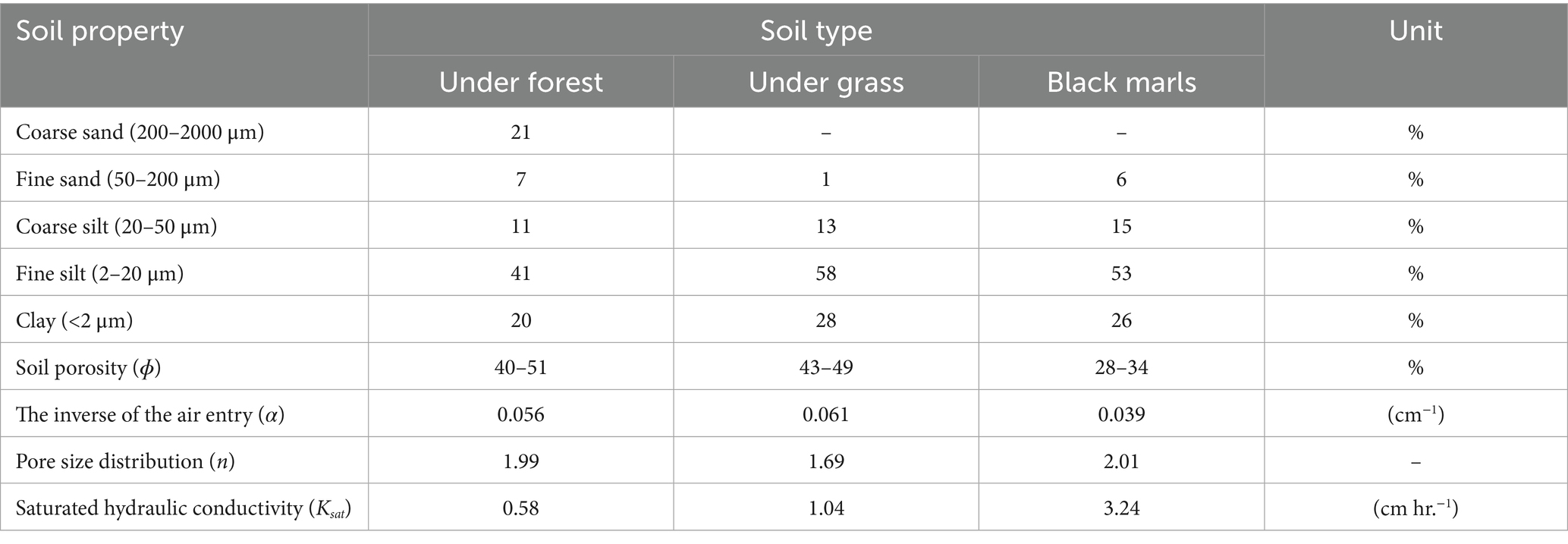
Table 1. Soil physical properties at the Moulin-Laval divide.

Building on the analysis of soil physical properties, it is also essential to consider the mineralogical composition and infiltration behavior that influence soil structure and hydrological responses in the study area. The soils are composed of clay minerals, encompassing various types such as illite (12%), smectite/illite (31%), chlorite (6%), and kaolinite (5%) (Garel, 2010; Marc et al., 2017b). A fascinating observation during the research is the remarkable ability of rainwater to infiltrate through the soil crack system. This phenomenon of rainwater infiltration holds the key to diminishing the cohesion of the soil material and triggering inter-particle repulsion among the mineral particles.

3.2 Temperature calibration and correction

The FO-DTS temperature dataset at depths of 0, −5, −10 and −15 cm spans over the period from 2016 to 2017. The temperature record has been calibrated and corrected using two reference baths for the application and energy balance calculation (Section 3.2). The average, maximum and minimum temperature data collections are 11.28°C, 42.83°C, and −13.21°C, respectively (see Figure 2c). Observations of temperature profiles at four depths are sufficient to estimate the soil thermal diffusivity below the shallow surface according to Horton et al. (1983). The temperature profile during the observation period fluctuated significantly due to the presence of water from infiltration and evapotranspiration. Furthermore, the observed temperature responses along the fiber optic cable are consistent with previous field-scale studies using heated DTS systems. Notably, Striegl and Loheide (2012) demonstrated that temperature signals during passive and active heating can effectively infer soil moisture dynamics at high spatial resolution.

Figure 4 presents the results of calibrated and corrected temperature during the observations. Both the calibration and correction of temperature data were successfully carried out and both annual and diurnal temperature variation are clearly observed during the two-years. It is difficult to observe temperature variations during periods of precipitation. To infer local temperature variation due to rainfall events, signal processing was applied to extract the frequency component in the temperature records. Theoretically, the influence of soil water content variation is indicated as a random frequency. Moreover, temperature data also contains two very low frequencies corresponding to annual and diurnal temperature.

Figure 4

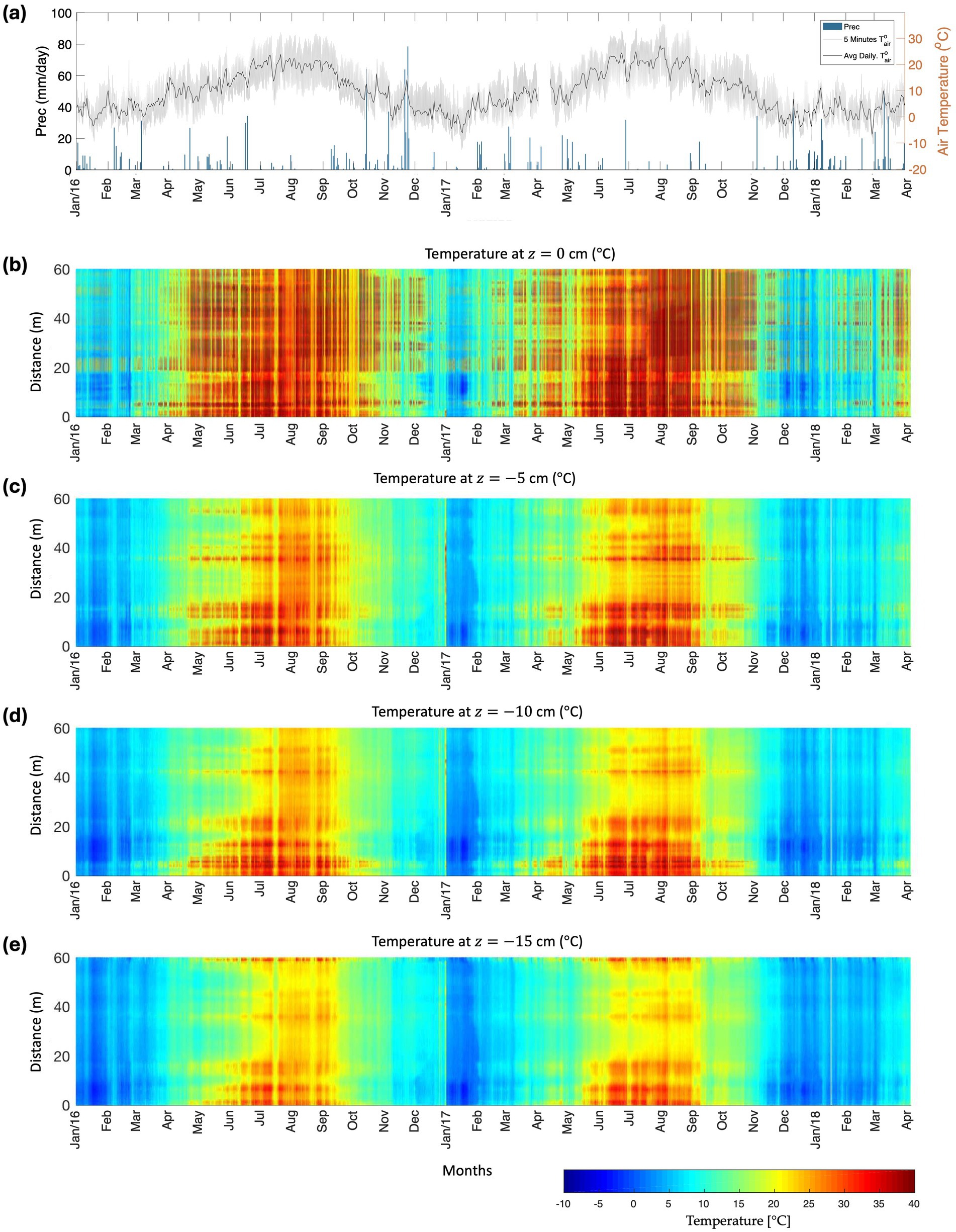
Figure 4. Rainfall, air and soil temperatures records at the Moulin-Laval divide. (a) Rainfall events and air temperature records. (b-e) Corrected long-term soil temperature profiles measured by FO-DTS during the observation period at depths of 0, −5, −10 and −15 cm.

The soil temperature profiles shown in Figure 4 indicate that temperature variations in topsoil are generally warmer and more variable than those at the subsurface. This observation supports the application of heat transfer equation for water detection. Furthermore, the measured temperature also shows a different character within each soil type, meaning that clay mineral types should be considered in the heat transfer application. For example, black marls are warmest in the summer but colder in the winter at depth. This indicates that black marls have the highest soil thermal diffusivity among the studied soil types. In areas that have a high content of interstratified Illite/Smectite, especially in black marls (31%), rainwater has the ability to infiltrate into the surface cracks network.

Furthermore, our findings are consistent with those of Striegl and Loheide (2012), who emphasized that the cable temperature response to heating strongly depends on soil moisture conditions. Our study observed that zones with higher soil moisture exhibited lower peak temperature responses and longer thermal recovery times, which agrees with their results. This behavior reflects wetter soils’ greater thermal conductivity and heat capacity, which dissipate the applied heat more effectively. These patterns confirm that passive heating in DTS systems can reliably capture spatiotemporal variations in soil moisture, supporting the broader applicability of this technique for long-term hydrologic monitoring.

3.3 Determination of soil thermal properties

Thermal parameters, such as soil heat capacity and thermal conductivity, are required in order to quantify the VWC of each soil type based on soil thermal diffusivity calculations (Béhaegel et al., 2007). Parameters are estimated using a nonlinear inversion of the Johansen model. We used 15 days of temperature and independent soil moisture observations for the period April 15–30, 2016. We conducted this procedure to infer the soil thermal properties, such as heat conductivity and heat capacity. Independent soil moisture probes were deployed on grassland at similar depths than the fiber optic cable (see Figure 2c). During the inversion, some rainfall events, and thus infiltration/drainage processes, occurred. Soil moisture variations ranging from 0.15 to 0.43 m³m⁻³ are included in this inversion step.

Figure 5 presents the parameter inferred from the Johansen model linking soil moisture and diffusivity. The circles are the observation data, and the solid line curve is the best mathematical model obtained from the inversion. The results of the inversion are optimized thermal parameters, i.e., soil heat conductivity $C_s=2.8$ MJm⁻³ K⁻¹, dry and saturated thermal conductivities ${\lambda }_d=0.53$ W m⁻¹. K⁻¹ and ${\lambda }_s=2.51$ Wm⁻¹ K^{−1, respectively.} The fitting analysis for the inversion results presents a goodness of fit with a $\mathit{\text{RMSE}}=9.8\times {10}^{-8}$ m²s⁻¹ with a coefficient of determination R² = 0.85.

Figure 5

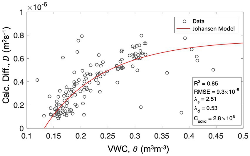
Figure 5. Soil thermal properties. The properties are determined using a nonlinear inversion of measured soil moisture (VWC) and calculated thermal diffusivity fitted to the Johansen model during a 15-day observation period; coefficient of determination R² = 0.85.

In agreement with the Johansen model, we fixed the soil thermal parameters to be applied uniformly across all soil types for the VWC calculations. Our hypothesis is based on the dominance of silt and fine clay in the soil composition (see Table 1). Consequently, we have attributed a single parameter value that adequately represents the thermal characteristics of the various soil types. This assumption ensures consistency and facilitates reliable VWC estimations throughout the analysis. These parameters may be insensitive to higher soil diffusivities in specific soil types and tend to introduce different error estimations, especially in almost saturated soils; however, low soil moisture can be inferred from low soil thermal diffusivity.

3.4 Implementation of the hybrid approach for VWC estimation

As discussed in section 3.1, the combination of a numerical simulation approach and of band stop filter as signal processing is used. This hybrid approach allowed determining the time series of soil thermal diffusivity. We used synthetic soil moisture variations generated by the Hydrus-1D software package as a synthetic simulation of changes in VWC. Nevertheless, the type of mineral should be considered to achieve realistic simulation.

3.4.1 Step 1: synthetic simulation of VWC

To generate a controlled reference for evaluating the estimation method, we conducted a synthetic simulation using the Hydrus-1D software package (Šimůnek et al., 2013). This simulation modeled volumetric water content (VWC) dynamics under simplified conditions, replicating field configurations at a depth of −15 cm, with output recorded every 6 min over 15 days. Hydrus 1D simulation estimate the VWC values at a depth of −10 cm to analyze a zone less influenced by rapid surface fluctuations. The soil hydraulic parameters were derived from typical properties of loamy soils. These parameters included a residual water content ( ${\theta }_r$ ) of 0.08 m³/m³, a saturated water content ( ${\theta }_s$ ) of 0.43 m³/m³, an air entry pressure ( $\alpha$ ) of 0.06 cm⁻¹, a pore size distribution ( $n$ ) of 1.9, and a saturated hydraulic conductivity ( $K_s$ ) of 21.2 cm/day.

In setting up the Hydrus-1D simulation, several assumptions were made to simplify the model and focus on evaluating the thermal response of soil to controlled moisture variations. First, the soil profile was assumed to be homogeneous, with uniform hydraulic properties throughout the depth. Second, it was assumed that atmospheric forcings such as surface temperature fluctuations, wind, and evapotranspiration have negligible influence at depths below −10 cm. This allowed us to isolate the influence of water input events on deeper soil layers without introducing surface-driven noise. Third, only controlled precipitation inputs were applied, two events on day 4 (1 cm/day) and day 9 (2 cm/day), while other meteorological variables such as rainfall, cloud cover, or air temperature were excluded. This was intended to simulate idealized conditions for assessing the temporal dynamics of VWC. Lastly, the simulation did not include root water uptake, assuming that vegetation effects were minimal or absent within the simulated timeframe and depth. These simplifications were essential to produce a clean synthetic dataset for evaluating signal processing methods for estimating soil VWC from temperature data (see Figure 6a).

Figure 6

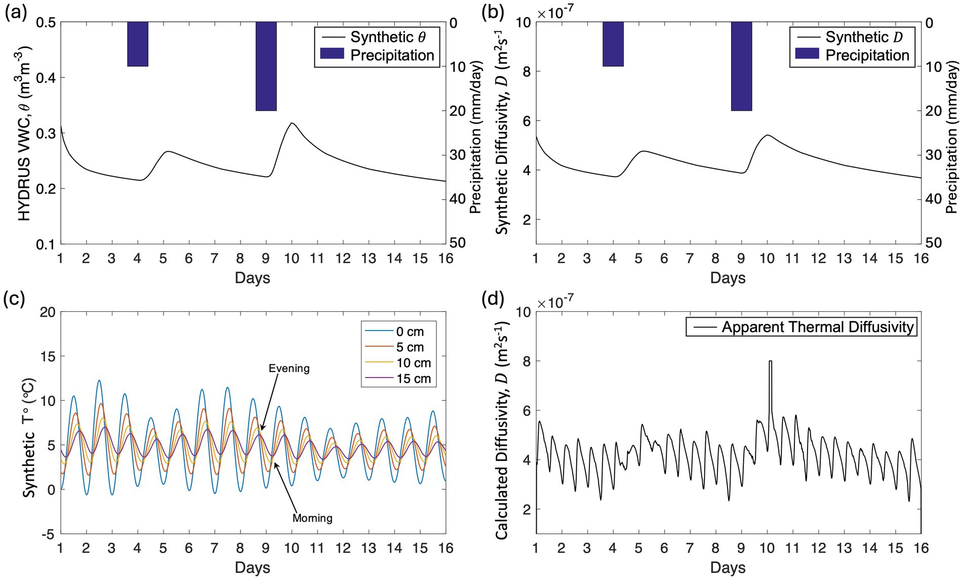
Figure 6. Results of the simulation and testing steps as a validation procedure. (a) Synthetic VWC generated with the Hydrus-1D software package. (b) Predefined soil thermal diffusivity converted from the Johansen model using synthetic VWC. (c) Synthetic temperature generated by considering the damping depth factor in Equation 3. Each point indicated by the arrow represents a very small difference of temperature in the morning and night. (d) Calculated soil thermal diffusivity containing the artifact and signature of VWC was explicitly determined using a finite difference approach with a calculated diffusivity.

VWC from the Hydrus-1D simulation predefines synthetic soil thermal diffusivity using the Johansen model with several estimated input parameters, such as soil porosity, heat capacity, and thermal conductivity. The parameters were extracted from the inversion results, as illustrated in Figure 6a. Additionally, we adopted a soil porosity of 47%, which aligns with previous research conducted by Mallet (2018) about the study site. Figure 6b presents times series of predefined soil thermal diffusivity as a function of synthetic VWC.

As shown in Figure 6c, the synthetic temperature was profiled at four depths with a 5 cm vertical spacing using the sinusoidal waveform in Equation 3 (Carslaw and Jaeger, 1959) and predefined soil thermal diffusivity corresponding to water change variations over 15 days. The profile exhibits small temperature differences in the morning and evening (see arrow in Figure 6c). This synthetic temperature dataset involved air temperature in order to attain plausible variations in soil temperature. The predefined diffusivity was then used to generate synthetic temperature profiles as shown in Figure 6c. Please note that although the qualitative observation of VWC’s signature is not seen in Figure 6c, the VWC change due to rainfall events can be clearly observed in Figure 6a. Therefore, the proposed method can effectively reacquire the apparent soil thermal diffusivity.

3.4.2 Step 2: recalculation of thermal diffusivity

This step aims to re-calculate the thermal diffusivity using a combination of numerical approaches and signal processing. The synthetic soil temperature in Figure 6c is used in a finite difference approach to obtain the calculated thermal diffusivity. Figure 6d, which presents the calculated thermal diffusivity involving diurnal variation at a depth of −10 cm, shows an artifact that appears twice a day when the temperature increases in the morning and decreases in the evening. After calculating thermal soil thermal diffusivity, the signature of water changes is not an obvious response in the diffusivity time series because the artifact dominates diffusivity on all days (Figure 6d). Therefore, a FFT is applied to investigate the artifact of calculated soil thermal diffusivity in the frequency domain and determine the filter design to remove undesirable frequencies. In this experiment, we verified the suitable cutoff frequency based on comparisons between predefined and filtered soil thermal diffusivities, which have a minimum residual error. By examining the cutoff frequency of the band stop filter, the suitable filter design for this experiment was found to be the Butterworth fifth-order filter and the normalized cutoff frequencies were $f_{\mathit{low}}=0.05$ and $f_{\mathit{\text{high}}}=0.11\times \pi$rad/samples (Figure 7a). However, we noted that the filter design might not be the same for other cases. The amplitudes of the filtered signal were attenuated during the filtering process such that the filtered soil thermal diffusivity might not represent the correct value. Therefore, the filtered signal seems to exhibit more ripple, but it has a similar temporal distribution (Figure 7b). In general, the thermal diffusivity of soil increases with the rainfall and thus water infiltration and decreases with drainage.

Figure 7

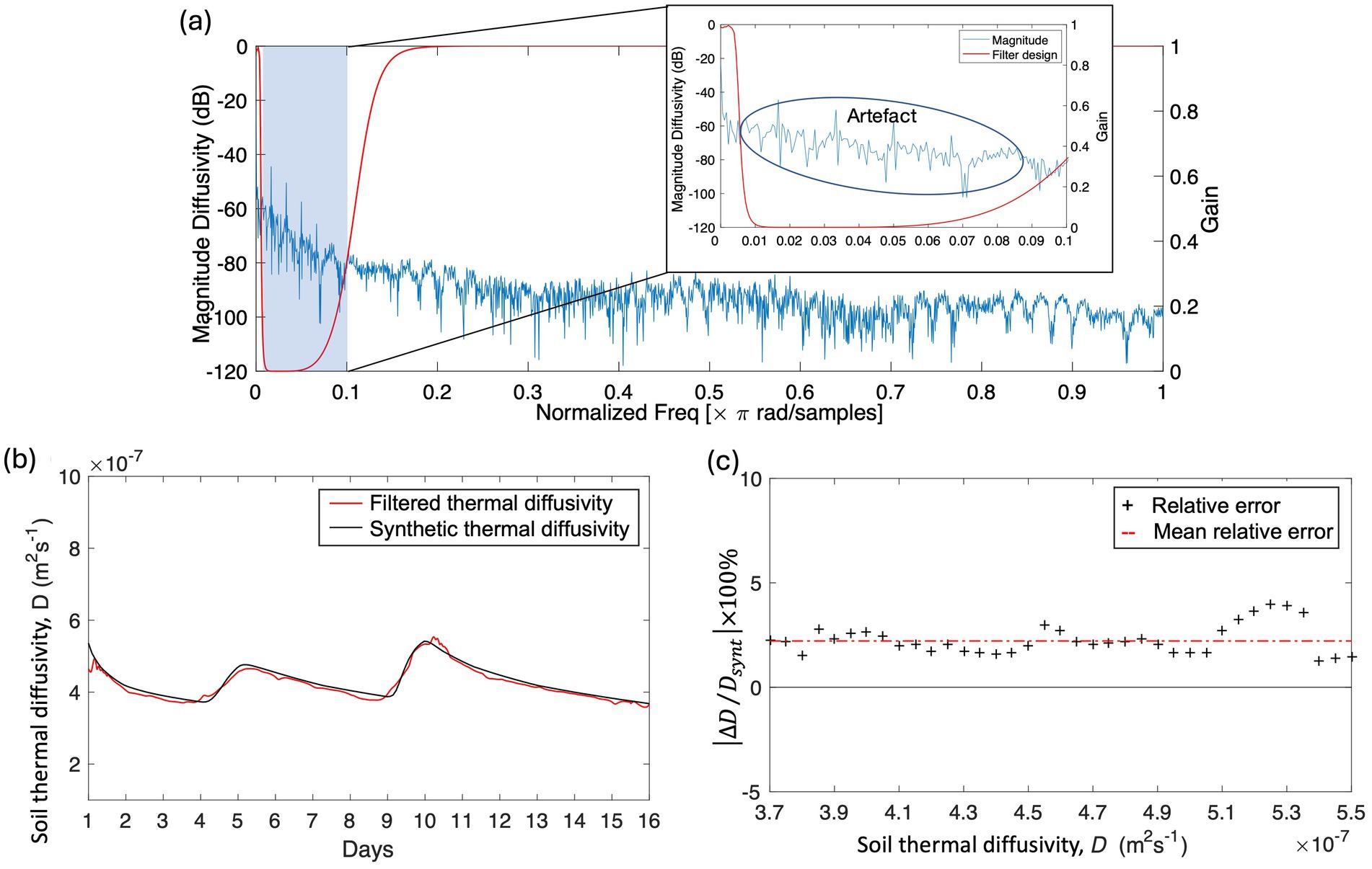
Figure 7. Calculated soil thermal diffusivity. The normalized cutoff frequencies were $f_{\mathit{low}}=0.05$ and $f_{\mathit{\text{high}}}=0.11\times \pi$rad/samples. (a) Implemented filter design in the normalized frequency domain for a period where the artefact was removed. (b) Comparison between filtered soil thermal diffusivity and predefined thermal diffusivity. (c) Percentage of mean relative error $\mid \mathit{\Delta D}/D_{\mathit{\text{synt}}}\mid$ between calculated and predefined soil thermal diffusivities with $\mid \mathit{\Delta D}\mid =\mid D_{\mathit{\text{synt}}}-D_{\mathit{\text{calc}}}\mid$ .

In addition, the signal-to-noise ratio of the filtered and synthetic signals demonstrated improvement during error analysis. Figure 7c shows the computation of the mean relative error between synthetic and calculated soil thermal diffusivity of the model experiment during a period of 15 days. The percentage of mean relative error of soil thermal diffusivity lies within the range of 3.7 × 10^-7 to 5.5 × 10^-7m².s⁻¹ while the total mean relative error for 15 days in the model is approximately 2.3%. The proposed method thus demonstrates fairly good performance and succeeds in determining soil thermal diffusivity without using the diurnal temperature period, as implemented in de Jong van Lier and Durigon (2013).

3.4.3 Step 3: calculation of VWC

This step consists in calculating the VWC (Figure 8a) by applying the filtered soil thermal diffusivity to the Johansen model. This was done in order to compare the calculated and synthetic VWC and investigate whether this procedure can be used in passive FO-DTS applications.

Figure 8

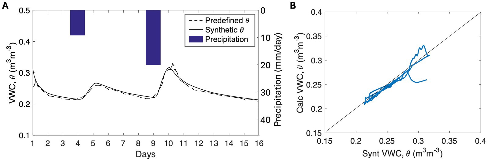
Figure 8. (a) Calculated VWC response overlapped with the synthetic VWC for two rainfall events. (b) Linear regression between calculated and synthetic VWC.

3.4.4 Step 4: validation of strategy

The final step is validation. This step consists in comparing the calculated VWC and synthetic VWC generated by Hydrus-1D; the fit among the two-time series has a mean relative percentage error value of 1.4%. The scatterplot in Figure 8b expresses the accuracy of the calculated VWC compared to synthetic VWC using linear regression. The calculated VWC has a fairly similar value compared to the synthetic value indicated by a coefficient of determination, R² = 0.92, and a Root Mean Square Error, RMSE = 0.06 m³m^-3.

3.5 Implementation of VWC calculation based on field experiments

This section describes the field implementation of the methodology for estimating VWC from soil thermal diffusivity at the clay-rich slopes of the Draix-Bléone catchment. After applying the explicit finite difference simulation and the signal filtering to the apparent soil thermal diffusivity, water content variation in the catena can be inferred. For example, the calculation for the period 15–30 April 2016 yields the apparent soil thermal diffusivity response shown in Figure 9a, further post-processed using an appropriate filter. The artifact presented by the red line appeared twice in each day. Moreover, soil thermal diffusivity was more frequently overestimated.

Figure 9

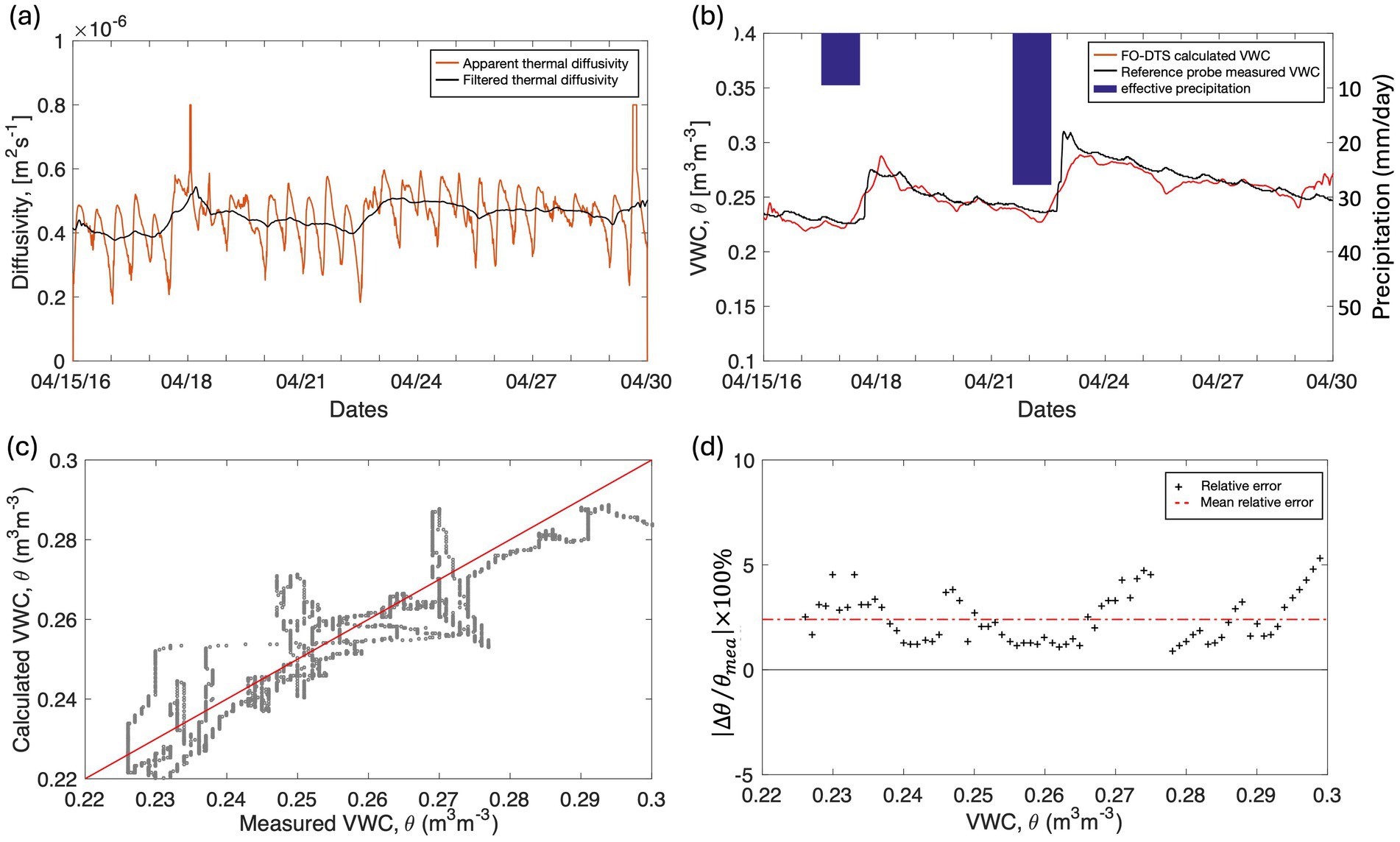
Figure 9. FO-DTS estimated thermal diffusivity and VWC versus reference soil moisture probe sensors for a period of 2 weeks, from 15 to 30 April 2016. (a) Calculated apparent and filtered soil thermal diffusivity based on FO-DTS soil temperature measurements. (b) FO-DTS calculated VWC versus reference soil moisture probe sensors. (c) Linear regression between FO-DTS calculated and reference probe measured VWC. (d) Percentage of mean relative error $\mid \mathit{\Delta \theta }/{\theta }_{\mathit{\text{measured}}}\mid$ between the calculated and reference probe measured VWC with $\mid \mathit{\Delta \theta }\mid =\mid {\theta }_{\mathit{\text{measured}}}-{\theta }_{\mathit{\text{calc}}}\mid$ .

To filter the artefact in the apparent soil thermal diffusivity response, the cutoff frequency was selected to fit to the variations in the VWC measured from the soil moisture probe. In field experiments, the cutoff frequency may not be the same for the various analyzed periods but maybe within a specific range of values. The band stop filter was designed according to the low-pass cutoff frequency range between 0.04 and 0.07 ( $\times \pi$rad/sample) and the high-pass frequency range between 0.1 and 0.13 ( $\times \pi$rad/sample). The black line in Figure 9a represents the filtered thermal diffusivity that performs acceptably for the field conditions (Figure 9b). The comparison and error analysis between the FO-DTS calculated VWC and the measured VWC are shown in Figures 9c,d. The mean relative error of the VWC calculation is approximately 2.2% for the period and variation of VWC due to infiltrating precipitation is revealed. The method is flexible as it allows to retrieve the measured variations in VWC, by adjusting a gain factor through normalization of the dry and saturated circumstances.

Figure 10a shows the measured soil moisture from 2016 to the end of 2017 as inputs to the inversion of the FO-DTS diffusivity for the three soil types. In this experiment, the depth of −10 cm corresponds to the Hydrus-1D simulation. The example period denoted by a red mark in Figure 10a was selected because it fits the dry and saturated conditions of the VWC. The maximum and minimum VWC during the studied period are 0.31 and 0.22 m³m⁻³, respectively (see Figure 9).

Figure 10

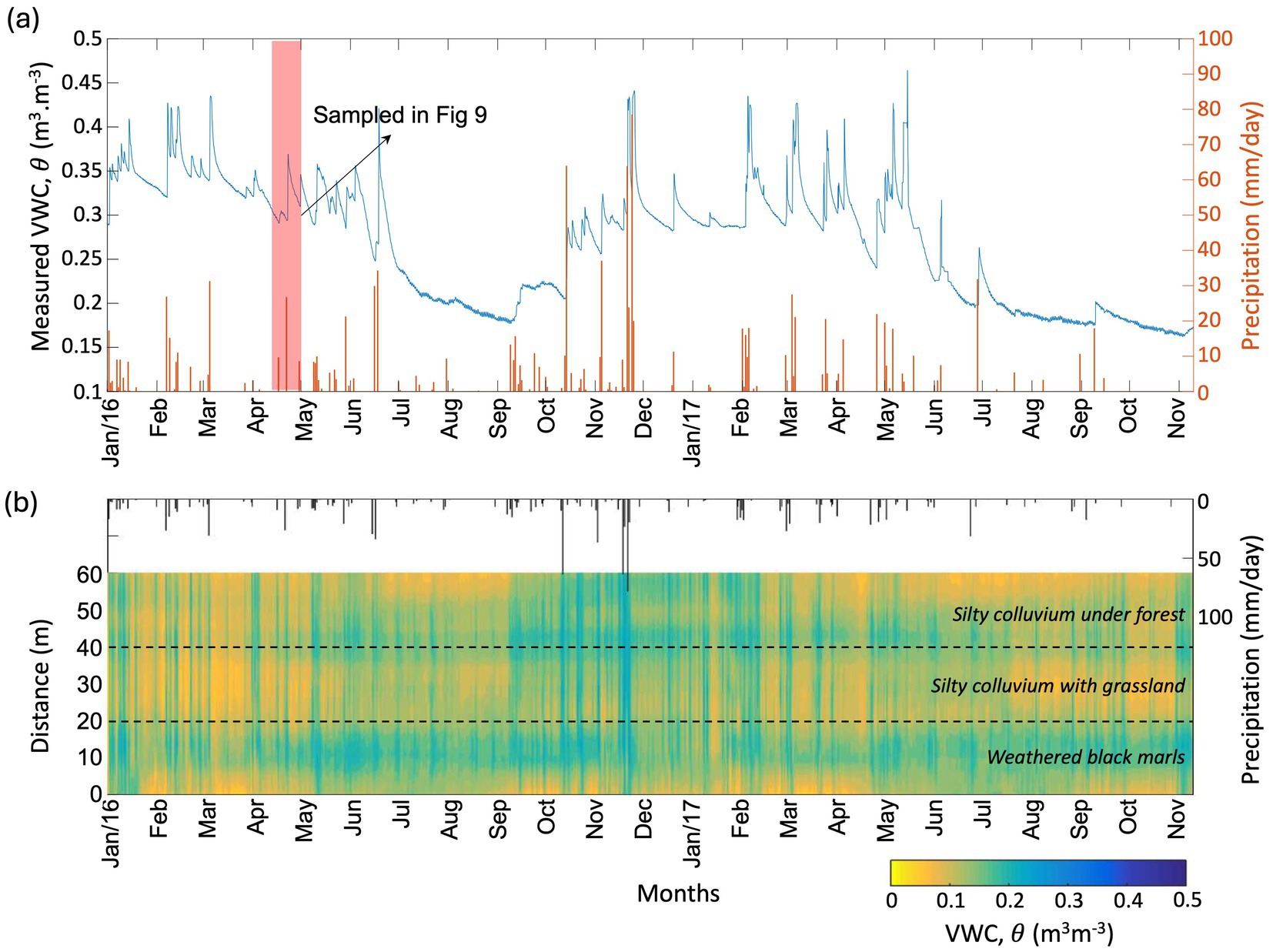
Figure 10. (a) VWC variations measured by the reference probe sensors during the period 2016–2017. (b) FO-DTS calculated VWC along the catena of three soil types and the precipitation. The response of the VWC calculation exhibits a delay of a few hours from the rainfall event peaks.

Soil thermal diffusivity calculations were performed for a period of 2 years based on the FO-DTS temperature measurements (see Figure 4) in order to estimate VWC variation under natural heat sources. The soil temperature observations provide insights in the presence of water although it was very difficult to determine changes when the temperature gradient is very small, especially during the winter season when the calculated VWC exhibits its highest values. During the summer season, the diurnal heat source is relatively high, and the FO-DTS calculated VWC changes is nicely depicted in relation to infiltrating precipitation and thus soil moisture increase.

The changes in FO-DTS calculated VWC are presented in Figure 10b for the period 2016–2017. The weathered black marls soil tends to retain the water longer than the silty colluvium under forest during the summer season. This is explained by the presence of roots that cause high transpiration in silty colluvium under forest cover. Conversely, the presence of clay in weathered black marls prevents water from undergoing evaporation. The soil under grass is drier than the weathered black marls soil after the summer period. Indeed, solar radiation directly permeated through the soil and sparse vegetation (leaves, herbs), which result in higher evapotranspiration rates. The presence of a root zone under the grass also explains these higher evapotranspiration rates. In summary, evapotranspiration in the silty colluvium with grassland is more intense than on the weathered black marls and on the silty colluvium under forest.

The proposed processing methodology considering both hydrodynamic numerical simulations and signal processing, allows to exploit high temporal and spatial resolutions temperature observations to retrieve soil thermal diffusivity as a function of VWC in the subsoils. The method avoids any phase lag and amplitude analysis, but possibility of calculation biases must be noted. The result of the VWC calculation might not exactly represent the true volumetric water content and the filtering has to be carefully designed according to reference soil moisture probe sensors. A calibration of the filter should be implemented, ideally, for each type of soil. It is also important to note that the processing parameters (e.g., cutoff frequency of the filter, soil heat properties) proposed in this work are specific to the conditions prevailing during the experiment.

4 Conclusion

This study addressed the challenge of monitoring long-term soil water dynamics in heterogeneous hillslope environments by developing a hybrid strategy using passive fiber-optic distributed temperature sensing (FO-DTS). The approach provides a minimally invasive alternative to conventional soil moisture measurement methods that often disturb soil structure and hydrological connectivity. Our process integrates high-resolution temperature observation with signal processing and finite-difference numerical modeling to estimate soil thermal diffusivity and derive volumetric water content at satisfactory spatial resolution (5 cm vertically and 50 cm horizontally) along a 60-meter soil catena. Several key findings emerged from this work. First, the spectral analysis of temperature time series proved effective in identifying temporal shifts in soil thermal behavior linked to moisture changes. Second, VWC estimation using temperature amplitude and phase delay performed well in capturing seasonal variations, with peak subsoil moisture depletion occurring during the summer due to increased evapotranspiration. Third, spatial heterogeneity in VWC distribution aligned with the three dominant soil types identified along the catena, confirming the influence of soil texture and structure on water storage capacity and infiltration behavior. Fourth, the 22-month dataset collected at 6-min intervals demonstrated the capacity of passive FO-DTS to capture both short-term and long-term soil moisture dynamics without requiring active heating or continuous power. These findings confirm the feasibility and value of using passive FO-DTS in field conditions with limited access to infrastructure. The method is particularly well suited for long-term, high-resolution soil hydrology studies in environments with strong seasonal climatic forcing. Future research should improve the accuracy of the inversion methods used for deriving VWC, account for root water uptake and dynamic boundary conditions, and expand the approach to steeper or more complex terrain. Ultimately, this work contributes to a deeper understanding of preferential flow, water redistribution, and soil–water interactions, essential for effective watershed management, erosion control, and long-term soil evolution under Mediterranean climate conditions.

Despite these promising results, several limitations should be acknowledged. The numerical simulation assumes homogeneous soil hydraulic properties and does not include processes such as root water uptake or dynamic atmospheric boundary conditions. The estimation of VWC from passive FO-DTS relies on indirect relationships between temperature signals and soil moisture, which introduces uncertainty, especially in the absence of direct validation using co-located in-situ moisture sensors. Moreover, variability in thermal conductivity across soil types may affect diffusivity estimations and introduce bias into the derived VWC values. These limitations highlight the need for further refinement and validation of the approach, particularly in more complex terrains or under varying climatic regimes. Overall, this work contributes to a better understanding of preferential flow, water redistribution, and soil–water interactions at high spatial and temporal resolution. It provides a basis for expanding minimally invasive, long-term soil moisture monitoring in Mediterranean environments and supports broader applications in hydrology, erosion management, and soil evolution studies.

Data availability statement

The raw data supporting the conclusions of this article will be made available by the authors, without undue reservation.

Author contributions

KS: Conceptualization, Data curation, Investigation, Methodology, Visualization, Writing – original draft, Writing – review & editing. J-PM: Conceptualization, Funding acquisition, Investigation, Resources, Supervision, Validation, Writing – review & editing. XC: Conceptualization, Formal analysis, Validation, Writing – review & editing. VM: Conceptualization, Formal analysis, Supervision, Validation, Resources, Writing – review & editing. JG: Conceptualization, Investigation, Resources, Software, Writing – review & editing.

Funding

The author(s) declare that financial support was received for the research and/or publication of this article. This work was part of the Research Infrastructure OZCAR/Draix-Bléone Observatory and has been financially supported by the project HYDROSLIDE (High frequency hydro) geophysical observations for a better understanding of landslides mechanical behavior, ANR-15-CE04-0009 and the project CRITEX (Challenging equipment for the spatial and temporal exploration of the critical zone, ANR-11-EQPX-0011) both funded by the French Research Agency (ANR).

Acknowledgments

The authors would like to thank INRAE/Draix-Bléone Observatory for the research opportunity.

Conflict of interest

The authors declare that the research was conducted in the absence of any commercial or financial relationships that could be construed as a potential conflict of interest.

Generative AI statement

The author(s) declare that no Gen AI was used in the creation of this manuscript.

Publisher’s note

All claims expressed in this article are solely those of the authors and do not necessarily represent those of their affiliated organizations, or those of the publisher, the editors and the reviewers. Any product that may be evaluated in this article, or claim that may be made by its manufacturer, is not guaranteed or endorsed by the publisher.

References

Adeniyi, M., and Oshunsanya, S. (2012). Validation of analytical algorithms for the estimation of soil thermal properties using de Vries model. Am. J. Sci. Ind. Res. 3, 103–114. doi: 10.5251/ajsir.2012.3.2.103.114

Crossref Full Text | Google Scholar

Anderson, M. P. (2005). Heat as a ground water tracer. Ground Water 43, 951–968. doi: 10.1111/j.1745-6584.2005.00052.x

PubMed Abstract | Crossref Full Text | Google Scholar

Antoine, P., Giraud, A., Meunier, M., and Van Asch, T. (1995). Geological and geotechnical properties of the “Terres Noires” in southeastern France: weathering, erosion, solid transport and instability. Eng. Geol. 40, 223–234. doi: 10.1016/0013-7952(95)00053-4

Crossref Full Text | Google Scholar

Bechkit, M. A., Flageul, S., Guerin, R., and Tabbagh, A. (2014). Monitoring soil water content by vertical temperature variations. Ground Water 52, 566–572. doi: 10.1111/gwat.12090

PubMed Abstract | Crossref Full Text | Google Scholar

Béhaegel, M., Sailhac, P., and Marquis, G. (2007). On the use of surface and ground temperature data to recover soil water content information. J. Appl. Geophys. 62, 234–243. doi: 10.1016/j.jappgeo.2006.11.005

Crossref Full Text | Google Scholar

Bense, V. F., Read, T., Bour, O., Le Borgne, T., Coleman, T., Krause, S., et al. (2016). Distributed temperature sensing as a down-hole tool in hydrogeology. Water Resour. Res. 52, 9259–9273. doi: 10.1002/2016WR018869

Crossref Full Text | Google Scholar

Bogena, H. R., Huisman, J. A., Oberdörster, C., and Vereecken, H. (2007). Evaluation of a low-cost soil water content sensor for wireless network applications. J. Hydrol. 344, 32–42. doi: 10.1016/j.jhydrol.2007.06.032

Crossref Full Text | Google Scholar

Campbell, G. S., Calissendorff, C., and Williams, J. H. (1991). Probe for measuring soil specific heat using a heat-pulse method. Soil Sci. Soc. Am. J. 55, 291–293. doi: 10.2136/sssaj1991.03615995005500010052x

Crossref Full Text | Google Scholar

Cao, D., Shi, B., Zhu, H., Wei, G., Chen, S. E., and Yan, J. (2015). A distributed measurement method for in-situ soil moisture content by using carbon-fiber heated cable. J. Rock Mech. Geotech. Eng. 7, 700–707. doi: 10.1016/j.jrmge.2015.08.003

Crossref Full Text | Google Scholar

Carslaw, H. S., and Jaeger, J. C. (1959). Conduction of heat in solids. 2nd Edn. New York, NY: Oxford Univiversity Press.

Google Scholar

Chavanne, X., and Jean-Pierre, F. (2014). Presentation of a complex permittivity-meter with applications for sensing the moisture and salinity of a porous media. Sensors 14, 15815–15835. doi: 10.3390/s140915815

Crossref Full Text | Google Scholar

Cheviron, B., Guérin, R., Tabbagh, A., and Bendjoudi, H. (2005). Determining long-term effective groundwater recharge by analyzing vertical soil temperature profiles at meteorological stations. Water Resour. Res. 41, 1–6. doi: 10.1029/2005WR004174

Crossref Full Text | Google Scholar

Chung, S. -O., and Horton, R. (1987). Soil heat and water flow with a partial surface mulch. Water Resour. Res. 23, 2175–2186. doi: 10.1029/WR023i012p02175

Crossref Full Text | Google Scholar

Cichota, R., Elias, E. A., and Van De Jong Lier, Q. (2004). Testing a finite-difference model for soil heat transfer by comparing numerical and analytical solutions. Environ. Model. Softw. 19, 495–506. doi: 10.1016/S1364-8152(03)00164-6

Crossref Full Text | Google Scholar

Ciocca, F., Lunati, I., Van de Giesen, N., and Parlange, M. B. (2012). Heated optical fiber for distributed soil-moisture measurements: a lysimeter experiment. Vadose Zone J. 11:199. doi: 10.2136/vzj2011.0199

Crossref Full Text | Google Scholar

de Jong van Lier, Q., and Durigon, A. (2013). Soil thermal diffusivity estimated from data of soil temperature and single soil component properties. Rev. Bras. Ciênc. Solo 37, 106–112. doi: 10.1590/S0100-06832013000100011

Crossref Full Text | Google Scholar

Dong, J., Agliata, R., Steele-Dunne, S., Hoes, O., Bogaard, T., Greco, R., et al. (2017). The impacts of heating strategy on soil moisture estimation using actively heated fiber optics. Sensors (Basel). 17, 1–11. doi: 10.3390/s17092102

Crossref Full Text | Google Scholar

Dong, J., Steele-Dunne, S. C., Judge, J., and van de Giesen, N. (2015). A particle batch smoother for soil moisture estimation using soil temperature observations. Adv. Water Resour. 83, 111–122. doi: 10.1016/j.advwatres.2015.05.017

Crossref Full Text | Google Scholar

Esteves, M., Descroix, L., Mathys, N., and Lapetite, J. M. (2005). Soil hydraulic properties in a marly gully catchment (Draix, France). Catena 63, 282–298. doi: 10.1016/j.catena.2005.06.006

Crossref Full Text | Google Scholar

Garel, E. (2010). Etude des processus de recharge des nappes superficielles et profondes dans les versants marneux fortement hétérogènes. Cas des Terres Noires des Alpes du Sud de la France—ORE Draix. Avignon: Université d’Avignon et des Pays de Vaucluse.

Google Scholar

Halloran, L. J. S., Rau, G. C., and Andersen, M. S. (2016). Heat as a tracer to quantify processes and properties in the vadose zone: a review. Earth-Sci. Rev. 159, 358–373. doi: 10.1016/j.earscirev.2016.06.009

Crossref Full Text | Google Scholar

Hartog, A. H., Belal, M., and Clare, M. A. (2019). Advances in distributed fiber-optic sensing for monitoring marine infrastructure, measuring the deep ocean, and quantifying the risks posed by seafloor hazards. Mar. Technol. Soc. J. 52, 58–73. doi: 10.4031/mtsj.52.5.7

Crossref Full Text | Google Scholar

Horton, R., Wierenga, P. J., and Nielsen, D. R. (1983). Evaluation of methods for determining the apparent thermal diffusivity of soil near the surface. Soil Sci. Soc. Am. J. 47, 25–32. doi: 10.2136/sssaj1983.03615995004700010005x

Crossref Full Text | Google Scholar

Kersten, M. (1949). Thermal properties of soils. Eng. Exp. Stn. Bull. 28, 1–226.

Google Scholar

Krarti, M., Claridge, D. E., and Kreider, J. F. (1995). Analytical model to predict nonhomogeneous soil temperature variation. J. Sol. Energy Eng. 117, 100–107. doi: 10.1115/1.2870823

Crossref Full Text | Google Scholar

Krzeminska, D. M., Steele-Dunne, S. C., Bogaard, T. A., Rutten, M. M., Sailhac, P., and Geraud, Y. (2012). High-resolution temperature observations to monitor soil thermal properties as a proxy for soil moisture condition in clay-shale landslide. Hydrol. Process. 26, 2143–2156. doi: 10.1002/hyp.7980

Crossref Full Text | Google Scholar

Liu, G., Meng, H., Qu, G., Wang, L., Ren, L., and Fang, L. (2023). Distributed optical fiber sensor temperature dynamic correction method based on building fire temperature-time curve. J. Build. Eng. 68:106050. doi: 10.1016/j.jobe.2023.106050

Crossref Full Text | Google Scholar

Loranger, S., Gagné, M., Lambin-Iezzi, V., and Kashyap, R. (2015). Rayleigh scatter based order of magnitude increase in distributed temperature and strain sensing by simple UV exposure of optical fibre. Sci. Rep. 5, 1–7. doi: 10.1038/srep11177

Crossref Full Text | Google Scholar

Lu, L., Wang, Y., Liang, C., Fan, J., Su, X., and Huang, M. (2023). A novel distributed optical fiber temperature sensor based on Raman anti-stokes scattering light. Appl. Sci. 13:20. doi: 10.3390/app132011214

Crossref Full Text | Google Scholar

Mallet, M. F. (2018). Spatialisation et modélisation de l’état hydrique des sols pour l’étude des processus de formation des écoulements en contexte torrentiel : application au bassin versant marneux du Laval (ORE Draix-Bléone, Alpes-De-Haute-Provence, France) (Issue 2018AVIG0055) [Université d’Avignon]. Available at: doi: https://theses.hal.science/tel-01914950

Google Scholar

Maquaire, O., Ritzenthaler, A., Fabre, D., Ambroise, B., Thiery, Y., Truchet, E., et al. (2002). Caractérisation des profils de formations superficielles par pénétrométrie dynamique à énergie variable: Application aux marnes noires de Draix (Alpes-de-Haute-Provence, France). Compt. Rendus Geosci. 334, 835–841. doi: 10.1016/S1631-0713(02)01788-1

Crossref Full Text | Google Scholar

Marc, V., Bertrand, C., Malet, J. P., Carry, N., Simler, R., and Cervi, F. (2017). Groundwater—surface waters interactions at slope and catchment scales: implications for landsliding in clay-rich slopes. Hydrol. Process. 31, 364–381. doi: 10.1002/hyp.11030

Crossref Full Text | Google Scholar

Mathys, N., Brochot, S., Meunier, M., and Richard, D. (2003). Erosion quantification in the small marly experimental catchments of Draix (Alpes de haute Provence, France). Calibration of the ETC rainfall-runoff-erosion model. Catena 50, 527–548. doi: 10.1016/S0341-8162(02)00122-4

PubMed Abstract | Crossref Full Text | Google Scholar

Mathys, N., Klotz, S., Esteves, M., Descroix, L., and Lapetite, J. M. (2005). Runoff and erosion in the black marls of the French Alps: observations and measurements at the plot scale. Catena 63, 261–281. doi: 10.1016/j.catena.2005.06.010

PubMed Abstract | Crossref Full Text | Google Scholar

McDaniel, A., Harper, M., Fratta, D., Tinjum, J. M., Choi, C. Y., and Hart, D. J. (2016). Dynamic calibration of a fiber-optic distributed temperature sensing network at a district-scale geothermal exchange borefield. Geo-Chicago 2016, 1–11. doi: 10.1061/9780784480137.001

Crossref Full Text | Google Scholar

McDaniel, A., Tinjum, J. M., Hart, D. J., and Fratta, D. (2018). Dynamic calibration for permanent distributed temperature sensing networks. IEEE Sensors J. 18, 2342–2352. doi: 10.1109/JSEN.2018.2795240

Crossref Full Text | Google Scholar

Oyewole, J., Olasupo, T., Akinpelu, J., and Faboro, E. (2018). Prediction of soil temperature at various depths using a mathematical model. J. Appl. Sci. Environ. Manag. 22:1417. doi: 10.4314/jasem.v22i9.09

Crossref Full Text | Google Scholar

Palmieri, L. (2014). Distributed optical fiber sensing based on Rayleigh scattering. Open Opt. J. 7, 104–127. doi: 10.2174/1874328501307010104

Crossref Full Text | Google Scholar

Rutten, M. M., Steele-Dunne, S. C., Judge, J., and van de Giesen, N. (2010). Understanding heat transfer in the shallow subsurface using temperature observations. Vadose Zone J. 9:1034. doi: 10.2136/vzj2009.0174

Crossref Full Text | Google Scholar

Sayde, C., Gregory, C., Gil-Rodriguez, M., Tufillaro, N., Tyler, S., Van De Giesen, N., et al. (2010). Feasibility of soil moisture monitoring with heated fiber optics. Water Resour. Res. 46, 1–8. doi: 10.1029/2009WR007846

Crossref Full Text | Google Scholar

Selker, J. S., Thévenaz, L., Huwald, H., Mallet, A., Luxemburg, W., Van De Giesen, N., et al. (2006). Distributed fiber-optic temperature sensing for hydrologic systems. Water Resour. Res. 42, 1–8. doi: 10.1029/2006WR005326

Crossref Full Text | Google Scholar

Seyfried, M., Link, T., Marks, D., and Murdock, M. (2016). Soil temperature variability in complex terrain measured using fiber-optic distributed temperature sensing. Vadose Zone J. 15, 1–18. doi: 10.2136/vzj2015.09.0128

Crossref Full Text | Google Scholar

Shang, Y., Sun, M., Wang, C., Yang, J., Du, Y., Yi, J., et al. (2022). Research progress in distributed acoustic sensing techniques. Sensors 22:16. doi: 10.3390/s22166060

PubMed Abstract | Crossref Full Text | Google Scholar

Sigmund, A., Pfister, L., Sayde, C., and Thomas, C. K. (2017). Quantitative analysis of the radiation error for aerial coiled-fiber-optic distributed temperature sensing deployments using reinforcing fabric as support structure. Atmos. Meas. Tech. 10, 2149–2162. doi: 10.5194/amt-10-2149-2017

Crossref Full Text | Google Scholar

Šimůnek, J., Šejna, M., Saito, H., Sakai, M., and Van Genuchten, M. T. (2013). The HYDRUS-1D software package for simulating the one-dimensional movement of water, heat, and multiple solutes in variably-saturated media. Riverside, CA: University of California.

Google Scholar

Smith, J., Brown, A., Demerchant, M., and Bao, X. (1999). Simultaneous distributed strain and temperature measurement. Appl. Opt. 38, 5372–5377. doi: 10.1364/AO.38.005372

PubMed Abstract | Crossref Full Text | Google Scholar

Steele-Dunne, S. C., Rutten, M. M., Krzeminska, D. M., Hausner, M., Tyler, S. W., Selker, J., et al. (2010). Feasibility of soil moisture estimation using passive distributed temperature sensing. Water Resour. Res. 46, 1–12. doi: 10.1029/2009WR008272

Crossref Full Text | Google Scholar

Stevanato, L., Baroni, G., Cohen, Y., Lino, F. C., Gatto, S., Lunardon, M., et al. (2019). A novel cosmic-ray neutron sensor for soil moisture estimation over large areas. Agriculture 9:202. doi: 10.3390/agriculture9090202

Crossref Full Text | Google Scholar

Striegl, A. M., and Loheide, S. P. (2012). Heated distributed temperature sensing for field scale soil moisture monitoring. Ground Water 50, 340–347. doi: 10.1111/j.1745-6584.2012.00928.x

PubMed Abstract | Crossref Full Text | Google Scholar

Suárez, F., Hausner, M. B., Dozier, J., Selker, J. S., and Tyler, S. W. (2011). Heat transfer in the environment: Development and use of fiber-optic distributed temperature sensing. London: IntechOpen.

Google Scholar

Tabbagh, A., Cheviron, B., Henine, H., Guérin, R., and Bechkit, M. A. (2017). Numerical determination of vertical water flux based on soil temperature profiles. Adv. Water Resour. 105, 217–226. doi: 10.1016/j.advwatres.2017.05.003

Crossref Full Text | Google Scholar

van de Giesen, N., Steele-Dunne, S. C., Jansen, J., Hoes, O., Hausner, M. B., Tyler, S., et al. (2012). Double-ended calibration of fiber-optic raman spectra distributed temperature sensing data. Sensors 12, 5471–5485. doi: 10.3390/s120505471

PubMed Abstract | Crossref Full Text | Google Scholar

van Genuchten, M. T. (1978). Calculating the unsaturated hydraulic conductivity with a new, closed-form analytical model. Princeton, NJ: Princeton University.

Google Scholar

Van Wijk, W. R., and Derksen, W. J. (1966). Thermal properties of a soil near the surface. Agric. Meteorol. 3, 333–342. doi: 10.1016/0002-1571(66)90015-x

PubMed Abstract | Crossref Full Text | Google Scholar

Weiss, J. D. (2003). Using fiber optics to detect moisture intrusion into a landfill cap consisting of a vegetative soil barrier. J. Air Waste Manag. Assoc. 53, 1130–1148. doi: 10.1080/10473289.2003.10466268

PubMed Abstract | Crossref Full Text | Google Scholar

Wu, J., and Nofziger, D. L. (1999). Incorporating temperature effects on pesticide degradation into a management model. J. Environ. Qual. 28, 92–100. doi: 10.2134/jeq1999.00472425002800010010x

Crossref Full Text | Google Scholar

Zhang, Z. F. (2017). Should the standard count be excluded from neutron probe calibration? Soil Sci. Soc. Am. J. 81, 1036–1044. doi: 10.2136/sssaj2017.02.0052

Crossref Full Text | Google Scholar

Zhou, D. P., Li, W., Chen, L., and Bao, X. (2013). Distributed temperature and strain discrimination with stimulated brillouin scattering and rayleigh backscatter in an optical fiber. Sensors 13, 1836–1845. doi: 10.3390/s130201836

PubMed Abstract | Crossref Full Text | Google Scholar

Zhu, Y., Irmak, S., Jhala, A. J., Vuran, M. C., and Diotto, A. (2019). Time-domain and frequency-domain reflectometry type soil moisture sensor performance and soil temperature effects in fine- and coarse-textured soils. Appl. Eng. Agric. 35, 117–134. doi: 10.13031/aea.12908

Crossref Full Text | Google Scholar