IoT enabled smart water metering using multi sensor data and machine learning techniques

Water Distribution Systems (WDS) are critical infrastructure assets that deliver water from source to consumers. The increasing scarcity of fresh water has heightened the importance of monitoring these systems. Conventional smart metering solutions require intrusive installation in pipelines, increasing costs and complexity. Moreover, in intermittently operated networks, which are common in India and other countries of the global south, the line is not pressurized for considerable amounts of time, resulting in poor performance of conventional water meters. Periodic maintenance of these meters can cause similar disruptions. This study introduces a novel non-intrusive technique for WDS monitoring by measuring water consumption, offering a cost-effective alternative to existing smart meters. The system can be effectively built, including installation, at a fraction (1/10^th) of the cost of existing smart meters. The proposed technique utilizes low-cost level sensors in OverHead Tanks (OHTs), sumps or reservoirs, which are used in many cities, towns, and villages in the global south to cope with the intermittent supply. Two estimation approaches are explored: predefined flow rates from baseline experiments and a dynamic method that adapts to variations in tank level. The methodology is validated through controlled experiments and from actual operating systems, demonstrating its effectiveness in handling fluctuations in inflows and intermittent outlet flows. Results show that while predefined flow rates offer accuracy in stable conditions, dynamic estimation is more adaptable to real-world variability. This approach enables scalable and affordable smart water monitoring, contributing to sustainable water management.

1 Introduction

Water Distribution Systems (WDS) are critical and essential infrastructure assets that deliver water from storage reservoirs or treatment plants to consumers. A typical WDS consists of a network of pumps, pipes, storage tanks and valves that are operated to meet the water demand of residential, commercial, and industrial users. The effective maintenance of the WDS is vital for sustainable water management, which can be achieved by monitoring and making informed decisions, especially in regions facing water scarcity (Hejazi et al., 2023; Ullah et al., 2023). At least 2 billion people on the planet face water scarcity at some point in the year, and these numbers are expected to grow to 2.8 billion by 2030 as water availability decreases (United Nations, 2022). In the last two decades, the water sources on land and in the subsurface, including ice and snow, have dropped at a rate of 1 cm per year, which is higher than the total human water consumption per year. This greatly impacts the fact that only 0.5% of the Earth's water is usable and available as freshwater. Sustainable Development Goal (SDG) 6, established by the General Assembly of the United Nations, aims to ensure that everyone has access to clean water and sanitation by 2030 (WMO, 2021). At the current rate of progress, the world will achieve only 81% coverage by 2030. This shortfall will leave 1.6 billion people without safe managed drinking water supplies, which requires a four-fold increase in the pace of progress to meet the target. Countries in the global south, such as India, are considered water-stressed with a per capita availability estimated at 1,567 m³ (Ministry of Jal Shakti, 2024). The percentage of urban population covered by piped water systems varies from 53 to 71%, and the water supply per capita varies from 70 to 112 lpcd (liters per capita per day), with water supply limited to 4-6 h. The percentage of metered connections is 48% in the larger cities, whereas there are very few or no metered connections in the smaller cities and towns (Indian Infrastructure, 2023). Supply is intermittent, with actual supply only about 1.5-3 h a day (Vairavamoorthy et al., 2008; Chinnusamy et al., 2018a). Leaks, amounting to almost 50% in some networks result in gross inefficiencies due to the loss of water and energy and have negative impacts on water quality, especially in intermittently operated networks (Spedaletti et al., 2022).

Accurately measuring water usage and availability enables better planning and management of water resources. It helps in detecting leaks, promoting usage awareness and encouraging sustainable practices. Effective measurement ensures informed decision making, supports policy development and facilitates crisis management during droughts or shortages. While water scarcity is a significant issue, measuring water use is far from straightforward. The typical method to measure domestic water use is through traditional water meters, which typically provide limited information on total consumption over time. Monitoring becomes challenging due to the lack of data to detect leaks and anomalies. Consequently, there is a need to transition from such basic systems toward smart metering approaches by digitalizing the data, enabling better data analysis and informed decision-making for sustainable water use. Existing smart meters store data digitally and provide detailed information on water usage patterns (Madias et al., 2023). One such system integrates Electronic Interface Modules (EIMs) with existing mechanical water meters and transfers data via smartphone interfaces or routers to the cloud, providing a solution for digitizing water usage data (Suresh et al., 2017). This allows for better monitoring, quicker leak detection, and more informed decision-making by providing precise data, which can be analyzed to optimize water usage and address issues promptly, making them more effective tools for managing water resources (Madias et al., 2022). However, these smart meters are often intrusive, requiring installation within the plumbing system, which can be disruptive and may need professional installation. Intrusive smart water meter installations should comply with industry standards such as Indian Standards IS 779 (Bureau of Indian Standards, 1994), or International Organization for Standardization ISO 4064 (International Organization for Standardization, 2014), or American Water Works Association C700 (American Water Works Association, 2020). These require specific flow-conditioning and installation elements to ensure accuracy, including U-shaped pipe loops or flow straighteners or long and straight runs of pipe both upstream and downstream of the meters. To protect the meters from debris, strainers are installed upstream, and to stop any backflow disrupting the meters, non-return valves or check valves are installed downstream, which increases the capital cost and creates a barrier to scalable deployment (Richard Koech and Syme, 2021).

In many cities, towns, and villages in the global south, users cope with the intermittent supply with intermediate storage facilities such as tanks, sumps, or reservoirs. In intermittently operated WDS, intermediate overhead tanks or elevated reservoirs have separate inlets and outlets, i.e., they are filled by pipes connected to their top, and the withdrawal is made through pipes connected to their bottom (Kurian et al., 2023). It is important for utility operators to monitor both the inlet volume of water entering reservoirs or overhead tanks (OHTs) and the outlet volume consumed from them (Sankar et al., 2015) for balancing the water supply and demand by appropriate scheduling. Such smart water meters require separate installations on both the inlet and outlet pipelines, effectively doubling the installation and maintenance costs.

Several notable approaches have been proposed to enable non-intrusive monitoring of fixture-level water usage without extensive modifications to existing plumbing systems. Among these, NAWMS (Nonintrusive Autonomous Water Monitoring System) is an augmented metering framework that infers water usage of individual pipelines by combining measurements from an inline water meter at the network inlet and clamp-on vibration sensors installed on each pipe section (Kim et al., 2008). These sensors detect vibration signatures generated by water flow, which are then mapped to the total flow using an information-fusion algorithm. The authors propose a two-phase optimization framework, leveraging linear programming and geometric programming, to automatically calibrate the vibration sensors. Another notable system, HydroSense, installs a single pressure sensor at an accessible point, such as a tap or drain, to record transient pressure spikes caused by fixture usage (Froehlich et al., 2009). During the training phase, the system learns the pressure patterns and corresponding average flow volumes for each fixture. A probabilistic classifier then disaggregates the pressure data into individual events and estimates fixture-level usage. Extending this idea, WATTR introduces self-powered wireless tags that harvest energy from pressure pulses in the pipe to power themselves and detect flow (Campbell et al., 2010). While these systems achieve approximately 90% accuracy in controlled indoor environments, they often require dense sensor deployments and extensive training phases. A broader survey in Abu-Bakar et al. (2021) summarizes these and other non-intrusive technologies, highlighting their promise but also the challenges in deploying them reliably at scale in real-world distribution networks.

Despite their promise, these approaches are predominantly designed for indoor settings or require dense sensor deployments and complex training procedures. Moreover, they are not directly applicable to infrastructure commonly found in low- and middle-income regions, such as overhead tanks and sumps where water is supplied intermittently and stored for later consumption. This highlights the need for scalable, low-cost, and infrastructure-light methods tailored to the dynamics of such systems.

This study aims to develop non-intrusive techniques for accurately estimating both the total volume of water supplied and consumed without the need for direct flow meter installations on pipelines. This is achieved by leveraging cost-effective sensors in OHTs, sumps or reservoirs that monitor water levels and auxiliary signals ensuring minimal disruption to existing infrastructure. To ensure data reliability, advanced filtering techniques are applied to address issues such as noise and outliers common in low-cost sensors. Auxiliary information is also utilized to infer flow, especially under simultaneous inlet and outlet conditions. From these water-level trends and auxiliary variables, flow rates are estimated using two methods. The first method used pre-determined flow rates that can be interpreted as a supervised learning approach when ground truth flow data is available during the training phase. The second method can be interepreted as an unsupervised inference method where consumption or supply is inferred dynamically without labeled data. The methodology is validated through multiple case studies, spanning scenarios with synchronous inlet and outlet flows, variable demand patterns and both controlled and uncontrolled conditions. Flow sensor readings serve as a baseline to compare the performance of the methods. Comparisons between the two methods highlight the method's adaptability and learning potential in real-world settings.

2 Materials and methods

2.1 System description

In intermittently operated networks, overhead tanks, sumps, and reservoirs are commonly used to accommodate discrete supply schedules. These storage structures typically have separate inlet and outlet pipelines. Water is supplied for a limited period of time and is stored in overhead tanks, sumps, or reservoirs. The stored water is consumed during the day and is drawn by gravity (from overhead tanks) or pumped from sumps or ground-level or underground reservoirs.

2.2 Data acquisition and communication

To monitor parameters in the Water Distribution System (WDS), various sensors are used to convert physical signals into electrical data. The primary measurements considered in this study include tank level and auxiliary indicators of flow status.

• Water level data: water level of the tank is the primary measurement used in this study. In case study 2 of the Section 3, DF Robot's Gravity: Industrial Stainless Steel Submersible hydrostatic Level Sensor (0 to 500 cm H₂O ± 0.5% full-scale error) is used to determine the height of water in OHTs. These level sensors provide critical data for managing water supply and consumption by measuring the pressure exerted by the water column (Zhou et al., 2020), which is then translated into the water level. This sensor has a rated service life of 1 × 10⁸ pressure cycles, effectively ensuring long-term mechanical reliability (DFRobot, n.d.). Potential sensor drift over time due to physical wear or electrical aging can be addressed through biennial calibration. The calibration can be done using the sensor interface unit. The process of converting the current signals from the sensor to voltage is done by a current-to-voltage converter, which has two potentiometers to adjust the zero and span of the voltage output. When the tank is empty, the zero potentiometer is adjusted to set the voltage to 0. At the maximum fill level, the span can be adjusted to make the current-to-voltage converter's output correspond to the actual level. This can be done at site by locally trained electricians with minimal equipment.

Alternatively, ultrasonic level sensors can also be used (Ding et al., 2025; Cherqui et al., 2020). In this study, the HC-SR04 ultrasonic level sensor (2 to 400 cm ± 0.3 cm), is employed in Case Study 1 of the Section 3 for indoor laboratory settings, while the MB7566 SCXL-MaxSonar-WR (50 to 1,000 cm ± 1% full-scale error), which is more suitable for outdoor installations, is used in case study 3. Ultrasonic sensors deliver non-contact sensing with ≤ 1% full-scale error but require proper mounting distance, temperature compensation, echo filtering, and periodic calibration. In contrast, hydrostatic level sensors can directly measure the pressure of the water column are less prone to errors, have built-in temperature compensation but require additional circuitry to convert the current to voltage for interfacing them with microcontrollers (Mohindru, 2023).

• Auxiliary data: in addition to level sensors, auxiliary data such as valve and pump status play a crucial role in inferring water flow dynamics. By analyzing when valves are actuated or pumps are operational, the periods of water supply or withdrawal can be determined, thereby enabling more accurate flow estimation especially during intervals when both inlet and outlet flows occur simultaneously. In practical deployments, valve status can be obtained using digital control systems that log actuation events or through wired connections to the valve actuator. Pump status can be inferred either from the electrical contactor of the pump or through power monitoring using energy meters installed on the pump line. Alternatively, independent sensor modules can be deployed to collect auxiliary information. For example, MPU6050-based vibration sensors can be mounted directly on pipelines to detect flow-induced vibrations. By isolating these vibration patterns from background noise, the presence of flow can be confirmed and even correlated with flow rate magnitudes (Ismail et al., 2014). These auxiliary signals are essential for correctly identifying flow activity, particularly when direct flow sensors are absent.

• Digitization and communication: the interface unit plays a critical role in connecting the sensors to the data communication network. At its core is an ESP8266 microcontroller, which collects data from various sensors, including level sensors and other auxiliary sensors and transmits it to a nearby gateway–also an ESP8266–using the ISM radio band. This gateway then relays the real-time data to the cloud via integrated WiFi, ensuring up-to-date monitoring for timely interventions and effective management (Chinnusamy et al., 2018b; Raphael and Narasimhan, 2022; Raphael et al., 2024). The cloud platform used for this purpose is ThingSpeak, which enables real-time visualization and analytics of the sensor data (MathWorks, n.d.a). To ensure secure access and protect the integrity of the transmitted data, the system supports HTTPS-based communication and requires authenticated API keys (MathWorks, n.d.b). This architecture is particularly advantageous for multi-sensor setups, enabling efficient data communication and centralized control. The high-level communication architecture is shown in Figure 1.

Figure 1

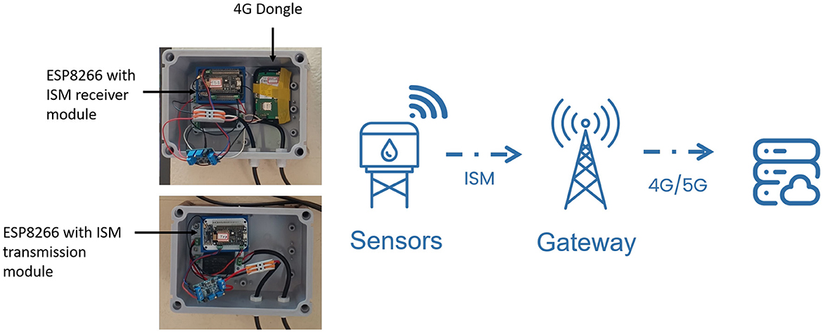
Figure 1. Interface unit and a high level communication architecture.

Any existing air vent on the roof of the tank or sump can be utilized for installing these level sensors. For hydrostatic sensors, the probe is submerged vertically to the bottom of the tank or sump. In the case of ultrasonic sensors, the device is mounted on the ceiling of the tank or sump, facing downward at 90 degrees. A shielded multicore cable is used to supply power and transmit sensor readings to the Interface Unit, which handles signal digitization and communication. This Interface Unit is installed at an accessible location to allow for future calibrations and is powered using a nearby AC mains source. To obtain the pump status, the NO (Normally Open) terminals of the electrical contactor are connected to the interface unit, which act as a simple switch and closes the circuit when the contactor is energized. Alternatively, a Non-Invasive current transformer can be installed in the power line of the pump, which measures the current passing through the wire. The Non-Invasive current transformer is connected to the Interface unit, which is then converted to a binary decision (Pump is ON if the measured current is greater than 0 A). The entire installation process can be carried out by local technicians with ease. Furthermore, the modular architecture and accessible placement of components significantly reduce the burden of long-term maintenance, allowing routine inspections, recalibrations and part replacements to be conducted without dismantling the system. This supports long term sustainability of the system and capacity-building through community-level technical involvement.

In this study, level sensors serve as the primary data source, while valve status or pump status act as the key auxiliary parameters. We aim to validate the non-intrusive parameter estimation method, ensuring accurate measurement of water consumption and effective monitoring of the water distribution system.

2.3 Level data pre processing

One of the most critical steps in water flow estimation is determining whether the tank level is increasing or decreasing after processing the sensor data. Raw sensor data are noisy and this variation can obscure true trends, making it difficult to estimate flow rates accurately. To address this, smoothing techniques such as ℓ₁ trend filtering are employed to reduce fluctuations and provide a clearer representation of water level changes (Kim et al., 2009; Tibshirani, 2014).

ℓ₁ trend Filtering effectively reduces large variances while preserving underlying trends, allowing for a more algorithmically reliable estimation of water flow. It generates piecewise linear estimates through convex optimization based on the ℓ₁ norm. The optimization formulation minimizes residuals between estimated and actual data while ensuring that the result remains piecewise linear. This method is particularly valuable for level sensor data, where sudden spikes or drops in readings are improbable under normal conditions. Moreover, in intermittently operated networks, the level changes are typically piecewise linear with the individual trends corresponding to different modes of operation. The enhanced smoothing technique employs the objective function as in Equation 1:

$\begin{array}{ll}min||y-f(x)-u|{|}_1+\lambda ||Df(x)|{|}_1+\mu ||u|{|}_1& (1)\end{array}$

where:

• y: Original sensor data

• f(x): The trend function

• ||.||₁: The L1 norm (sum of absolute values)

• λ : Regularization parameter controlling the sparsity

• Df(x): Derivative of the trend function (encourages smoothness)

• u : The spike signal

• μ : Regularization parameter for the spike signal u.

The objective function balances two primary terms: the error term and the regularization term. The error term minimizes the difference between actual data points and the trend function, while the regularization term penalizes complex functions with large variations, encouraging sparsity. By adjusting the λ parameter, we can control the trade-off between fitting the data closely and maintaining a smooth, sparse trend. Although smoothing techniques help remove noise from sensor data, sudden spikes can still persist. To effectively isolate these spikes, an additional regularization term μ||u||₁ is introduced. This term specifically penalizes the complexity of the “spike signal” u, encouraging a solution with fewer, larger spikes that align with real-world expectations. Adjusting λ and μ, we can control the trade-off between fitting the data, maintaining a smooth trend and isolating spikes or outliers.

Intuitively, ℓ₁ trend filtering works by fitting straight-line segments to the data, allowing the slope to change only at a small number of points. This creates a piecewise linear approximation that preserves sharp transitions (if present) while removing high-frequency noise. Compared to classical smoothing methods such as moving averages or quadratic smoothing, ℓ₁ trend filtering is particularly well-suited for level sensor data where the underlying physical process is expected to be piecewise linear with occasional transitions. The original and filtered level sensor data from a typical observation are shown in Figure 2.

Figure 2

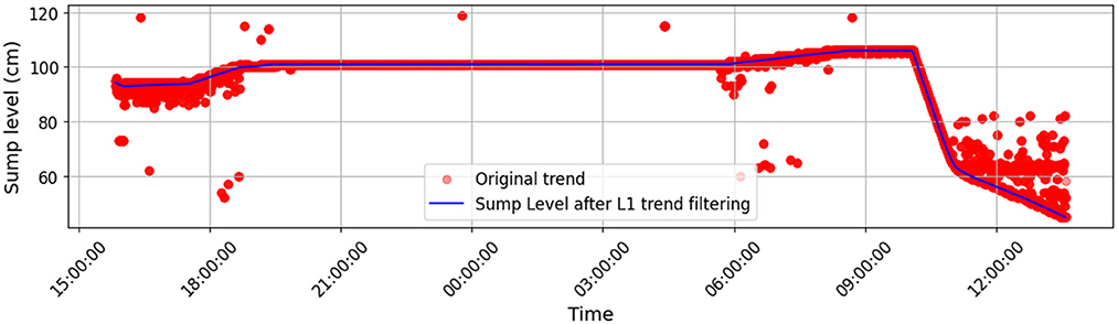
Figure 2. Original noisy level data (red points) compared with the denoised, piecewise-linear trend obtained using ℓ₁ trend filtering (blue line). The method preserves major structural changes while removing high-frequency noise, allowing more accurate flow estimation.

2.4 Methodology

We employ level sensors to continuously monitor the water level in overhead tanks or reservoirs. The change in the water level over a specific period allows us to calculate the volume of water entering or leaving the tank, which is described in Raphael and Narasimhan (2022). This methodology relies on the principle that the change in water level, when multiplied by the tank's cross-sectional area, provides an accurate measurement of changes in volume of water.

For instance, consider a tank with a known cross-sectional area A (in square meters). Let Δh(t) represent the change in water level (in meters) over a time interval Δt (in seconds). The change in height can be related to inflow (Q_in) and outflow Q_out as follows:

$\begin{array}{ll}\frac{A·\Delta h(t)}{\Delta t}=Q_{in}(t)-Q_{out}(t)& (2)\end{array}$

To compute water consumption as a temporal quantity, all positive and negative changes in water level must be considered over time. By measuring water levels at regular intervals and recording changes in height, the variation in water volume can be analyzed. The total volume over a given time period is calculated by summing up the instantaneous flow rates, where cumulative volume supplied V_in(T) and consumed V_out(T) is given in the Equation 3.

$\begin{array}{ll}{V}_{in}(T)={\displaystyle \sum _{t=0}^T}{Q}_{in}(t)\Delta t;V_{out}(T)={\displaystyle \sum _{t=0}^T}{Q}_{out}(t)\Delta t& (3)\end{array}$

When inlet and outlet are asynchronous, i.e., the supply and consumption periods do not overlap, V_in and V_out can be calculated as follows:

$\begin{array}{ll}{V}_{in}(T)={\displaystyle \sum _{t,\Delta h(t)>0}^T}{Q}_{in}(t)\Delta t;V_{out}(T)={\displaystyle \sum _{t,\Delta h(t)<0}^T}{Q}_{out}(t)\Delta t& (4)\end{array}$

However, when supply and consumption periods overlap, it is not straightforward to estimate the supply or consumption. In the following sections, we present two techniques to disambiguate the supply and consumption patterns from water level data.

2.4.1 Predefined flow rates

Accurately estimating water inflow and outflow using level sensors alone is challenging, particularly when both inlet and outlet flows occur simultaneously. In such cases, the net change in water level may not capture the underlying dynamics, making it difficult to infer the actual flow rates. This creates ambiguity, as the level sensor can only measure the overall effect of both flows rather than distinguishing between them. To overcome this limitation, it is necessary to integrate flow occurrence or directionality information with level change data, enabling a more reliable estimation of water movement.

To address this, we leverage auxiliary information from valve switch status or pump status. The key principle is that auxiliary data helps in knowing when the flow in inlet or outlet pipelines is active. This helps in resolving ambiguities and distinguishing the duration of when both the inlet and outlet flows occur simultaneously. This crucial information of the duration when both flows occur can be leveraged to use historical data where known flow rates are available to estimate the actual inlet and outlet flow rates separately. From a machine learning perspective, this process can be viewed as a simple form of supervised learning, where past labeled data (i.e., known flows during controlled events) is used to infer flows in unseen situations with similar auxiliary patterns.

By applying predefined flow values to these identified periods, we can improve the accuracy of flow estimation and mitigate errors that arise from overlapping flows. When auxiliary information, such as pump status or valve actuation, indicates that the inlet or outlet is active, the predefined flow rate is applied. The flow rate is calculated as:

$\begin{array}{ll}{Q}_{\text{in}}(t)=\{\begin{array}{ll}{Q}_{\text{pre, in}},\hfill & {\text{if Aux}}_{\text{in}}(t)=1\hfill \\ 0,\hfill & {\text{if Aux}}_{\text{in}}(t)=0\hfill \end{array}& (5)\end{array}$

$\begin{array}{ll}{Q}_{\text{out}}(t)=\{\begin{array}{ll}{Q}_{\text{pre, out}},\hfill & {\text{if Aux}}_{\text{out}}(t)=1\hfill \\ 0,\hfill & {\text{if Aux}}_{\text{out}}(t)=0\hfill \end{array}& (6)\end{array}$

where:

• Q_in(t) = Instantaneous inlet flow rate at time t

• Q_out(t) = Instantaneous outlet flow rate at time t

• Q_{pre, in} = Predefined inlet flow rate

• Q_{pre, out} = Predefined outlet flow rate

• Aux_in(t) = Auxiliary indicator for inlet at time t

• Aux_out(t) = Auxiliary indicator for outlet at time t

${\text{Aux}}_{\text{in}}(t)=\{\begin{array}{ll}1,\hfill & \text{if auxiliary data indicates inlet flow}\hfill \\ 0,\hfill & \text{if no inlet flow is indicated}\hfill \end{array}$

${\text{Aux}}_{\text{out}}(t)=\{\begin{array}{ll}1,\hfill & \text{if auxiliary data indicates outlet flow}\hfill \\ 0,\hfill & \text{if no outlet flow is indicated}\hfill \end{array}$

To determine these predefined flow rates (Q_{pre, in}, Q_{pre, out}), a separate baseline experiment is conducted where only one of the flows (either inlet or outlet) is active at a time. By measuring the resulting level change over a known period, the corresponding flow rate is calculated using Equation 2. Once both inlet and outlet flow rates are established through this controlled setup, it becomes possible to identify which one is lower in a given scenario.

For practical implementation, auxiliary data is utilized exclusively for the pipeline with the lowest flow rate in the system. As the occurrence of the higher flow rate will dominate the lower one, there will be a change in the tank level, which can be used as implicit auxiliary information for the higher flow rate.

Let two pipelines feed and draw from a tank of constant cross-sectional area A. Denote their instantaneous flow rates by

$Q_{in}(t),Q_{out}(t)\ge 0,$

and suppose w.l.o.g. that Q_in(t) ≤ Q_out(t) for all t in some interval I. The tank volume V(t) and level h(t) are related by V(t) = Ah(t). By mass-balance,

$\frac{dV}{dt}=Q_{in}(t)-Q_{out}(t)\Rightarrow A\frac{dh}{dt}=Q_{in}(t)-Q_{out}(t).$

Since by assumption Q_in(t) ≤ Q_out(t), it follows that

$\frac{dh}{dt}=\frac{Q_{in}(t)-Q_{out}(t)}{A}\le 0,$

with strict inequality whenever Q_out(t) > Q_in(t).

Thus:

(i) By monitoring the auxiliary signal on the pipeline with the lower flow (e.g., where Q_in occurs), we know exactly when Q_in(t)>0.

(ii) At times when the tank level is strictly decreasing, we can infer directly without (without any additional sensor) that the other outlet is active, i.e., Q_out(t) is active and in fact dominates.

Therefore, it suffices to install auxiliary sensors only on the pipeline with the lower flow. The behavior of the tank level itself reveals the activation of the larger flow through its decreasing trend.

In most cases of intermittent supply, where water is supplied for only a few hours in a day, the inlet and outlet flow rates are significantly different. E.g., if water from the source is stored in a tank or sump and is supplied itermittently to consumers, the inlet flow rate to the tank or sump would be significantly lower than the outlet. On the other hand, the inlet flow to a household sump or tank would be much higher than the consumption or outlet flow rate. However, in rare instances where they are, auxiliary data is required from both sides to determine the presence of flow and estimate the contribution of each. This ensures that even in cases where no significant net level change is observed, the underlying inflow and outflow can still be quantified. To further refine this estimation, additional sensor data can be incorporated. Sensors that detect flow movement, either through mechanical vibrations or other indirect methods, can help distinguish between an active inlet and an active outlet. These auxiliary data sources confirm whether water is entering or leaving the system, resolving cases where the level change alone is insufficient to determine flow direction.

The integration process follows these steps to accurately estimate water flow in ambiguous situations:

1. Monitor Level Changes: Continuously track water levels using sensors to detect fluctuations over time.

2. Determine the Flow Rate: Conduct a baseline experiment where only one flow (either inlet or outlet) is active at a time to establish predefined flow rates using the known cross-sectional area of the tank by Equation 2. Use this data to compare the inlet and outlet flows to identify which one is lower

3. Identify Flow Occurrence: Determine pipeline activity using auxiliary data like pump status or flow detection sensors.

4. Use Historical Flow Data: Once the pipeline activity is recorded, use predefined flow rates established in the baseline experiment to estimate its magnitude over the observed duration of its occurrence.

5. Compute Individual Flow Volumes: Using the estimated flow rate, calculate the inlet and outlet flow rates separately over time using Equations 5, 6 and finally the total volume by using Equation 3.

By combining level change measurements with flow occurrence data, a robust and accurate estimation of water movement is achieved. This approach ensures that even in scenarios where direct level changes are inconclusive, the presence or absence of flow provides the necessary validation to determine water distribution patterns accurately.

2.4.2 Dynamic flow rates

In real-world water distribution systems, flow rates are rarely constant and can fluctuate due to various factors, including network demand, infrastructure constraints, and environmental conditions. One major contributor to this variability is the nature of water sources and their supply dynamics. For instance, in many regions, water distribution relies on storage systems such as overhead tanks, which regulate supply to different areas. In water-scarce regions, particularly in South Asia, these OHTs are often filled using bore wells, introducing an additional layer of uncertainty. Bore well yield can vary significantly due to seasonal changes in groundwater levels, affecting the consistency of inflow (Choudhary and Singh, 2024; Minea et al., 2022; Shamsudduha et al., 2009). At the same time, the outlet flow rate remains unpredictable as it depends on network withdrawal patterns, which fluctuate based on demand and human behavior (Cassiolato et al., 2024). For this method to work effectively, one of the flow rates (either inlet or outlet) must remain relatively stable during the estimation period. This is because the approach relies on using the known flow rate and observed level changes to infer the unknown flow rate. If both the inlet and outlet flow rates vary unpredictably, the estimation becomes highly uncertain and may require additional measurements or advanced modeling techniques.

To estimate an unknown flow rate Q_u(t) using tank level measurements and the known flow Q_k(t). This unknown signal should ideally:

• Be consistent with the observed tank dynamics (mass balance),

• Vary smoothly or change slowly over time (since abrupt shifts in flow are rare in physical systems),

• Align with prior expectations, such as decreasing borewell yield or steady household demand.

A technique to estimate Q_u(t) under these assumptions is by formulating a convex optimization problem that enforces data fidelity and smoothness:

${\displaystyle \underset{Q_u(t)}{min}}{\displaystyle \sum _t}|s_k·A·\frac{dh(t)}{dt}+(Q_k(t)-Q_u(t))|+\lambda ·||\nabla Q_u(t)|{|}_1$

where

• s_k = +1 if Q_k(t) is the inlet flow and s_k = -1 if it is the outlet flow. This sign convention ensures that $s_k·A·\frac{dh(t)}{dt}$ correctly reflects the net contribution to tank level.

• h(t) is the observed (or denoised) tank level over time,

• $A·\frac{dh(t)}{dt}$ approximates the net flow derived from level change,

• ∇Q_u(t) is the discrete derivative (variation) of Q_u(t),

• λ is a regularization parameter balancing fit and smoothness.

This formulation closely resembles methods used in sparse signal recovery and regularized regression in machine learning. In particular, it aligns with the fused lasso or trend filtering models used to recover structured signals from noisy or partial observations. The minimization of a data fidelity term combined with an ℓ₁ penalty on the variation of the unknown signal is a common pattern in statistical learning. Thus, the estimation of Q_u(t) from tank level dynamics can be interpreted as a regression task, where we learn a structured, low-complexity approximation of the unknown flow signal using level data as a proxy.

Rather than solving this problem directly, we instead apply ℓ₁ trend filtering to the tank level data h(t). This produces a piecewise linear approximation ĥ(t), from which we derive the unknown flow rate as:

$Q_u(t)=Q_k(t)+s_k·A·\frac{d\widehat{h}(t)}{dt}$

This is, in fact, equivalent to solving the earlier convex program implicitly, because:

• ℓ₁ trend filtering enforces sparsity in the second derivative of h(t), leading to structured, piecewise-linear behavior,

• The derivative $\frac{d\widehat{h}(t)}{dt}$ yields a denoised, structured estimate of net flow,

• Subtracting from Q_k(t) provides a smoothed, implicitly regularized estimate of Q_u(t).

In discrete time, with sampling interval Δt, this yields:

$Q_u(t)=Q_k(t)+s_k·\frac{A}{\Delta t}·(\widehat{h}(t+\Delta t)-\widehat{h}(t)).$

This formulation reveals a deeper structural link: the temporal differences in Q_u(t) are directly proportional to the second-order differences in the filtered level trajectory h(t). Specifically,

$\begin{array}{r}\hfill Q_u(t+\Delta t)-Q_u(t)=s_k·\frac{A}{\Delta t}·(\widehat{h}(t+2\Delta t)-2\widehat{h}(t+\Delta t)+\widehat{h}(t))\\ \hfill =s_k·\frac{A}{\Delta t}·D\widehat{h}(t).\end{array}$

Taking ℓ₁ norms on both sides:

$||\Delta Q_u|{|}_1={\displaystyle \sum _t}|Q_u(t+\Delta t)-Q_u(t)|=\frac{A}{\Delta t}{\displaystyle \sum _t}|D\widehat{h}(t)|=\frac{A}{\Delta t}||D\widehat{h}|{|}_1.$

$\begin{array}{r}\hfill \begin{array}{||}\hline \Vert \Delta Q_u{\Vert }_1\propto \Vert D\widehat{h}{\Vert }_1\\ \hline\end{array}\Rightarrow {\ell }_{\text{1}}\text{ trend filtering on }h(t)\\ \hfill \text{implicitly regularizes }{Q}_u(t).\end{array}$

Thus, trend filtering on h(t) implicitly solves a fused-lasso problem on Q_u(t), achieving a structured and regularized flow estimate without requiring a separate optimization step. As a result, our method achieves a structured, smooth, and regularized flow estimate while avoiding a direct optimization step.

For practical implementation, the monitoring system should have the information:

• Known flow rate Q_k (either inlet or outlet)

• Tank level changes Δh(t)

• Time intervals Δt.

At any given time, the estimate of the unknown flow rate Q_u(t) is determined as:

$\begin{array}{ll}{Q}_u(t)=s_k·\frac{A·\Delta h(t)}{\Delta t}+Q_k& (7)\end{array}$

where:

• A is the cross-sectional area of the tank,

• Δh(t) is the observed change in water level,

• Δt is the time interval over which the change occurred.

The known flow rate Q_k is assumed to be approximately constant over short intervals. It can be determined either from isolated flow periods or, during simultaneous flows, by approximating it from stable regions immediately before or after a transition. Thus, Q_k reflects a locally constant flow rate rather than requiring strict isolation, making the approach applicable even in intermittently operated networks.

When both inlet and outlet flows occur simultaneously, periods of overlap are detected using auxiliary data such as pump or valve status. During these intervals, the unknown flow rate Q_u(t) is estimated dynamically using the known flow Q_k and the relationship in Equation 7. This enables accurate flow monitoring even under complex real-world conditions, where direct measurement of all flows may not be available. In the following, we assume that Q_out>>Q_in. The technique can be easily modified to accommodate the case when Q_out < < Q_in.

The dynamic algorithm (see Figure 3) operates by iterating through each time step of the level data and making inferences based on the observed trends and auxiliary conditions.

1. Start [Start at t = t_initial]: The process begins once a sufficient time window is available to compute a discrete slope.

2. Trend Detection [Is $\frac{\Delta h}{\Delta t}>0$?]: As seen in Figure 3a, the algorithm detects whether the tank level is increasing. This condition implies dominant inflow and minimal outflow.

3. Inflow Estimation [Estimate $Q_{\mathrm{\text{in}}}=A·\frac{\Delta h}{\Delta t}$]: When the level is rising, inflow is estimated directly from the slope of the water level curve assuming outflows are negligible.

4. Transition Check [Did slope change?]: The algorithm checks whether the sign of the slope has changed, i.e., $\left(\frac{\Delta h}{\Delta t}{|}_t^{t+\Delta t}·\frac{\Delta h}{\Delta t}{|}_{t-\Delta t}^t<0\right)$, to detect a turning point in the trend.

5. Known Flow Estimation [Compute $Q_{\mathrm{\text{out}}}=Q_{\mathrm{\text{in}}}(t_0)-A·\frac{\Delta h}{\Delta t}$]: At time t₀, the outflow is calculated using the previously estimated inflow. This value is stored as Q_k for use in future calculations.

6. Auxiliary Check [Auxiliary ON?]: If auxiliary systems (e.g., hidden inlets, pump actions) are active, the algorithm prepares to infer hidden inflows that would otherwise be unaccounted for.

7. Unknown Inflow Estimation [Infer Q_u(t)]: Using the stored Q_k, the unknown or hidden inflow is estimated as:

$Q_{\text{in}}^{\prime }(t)=Q_u(t)=Q_k-A·\frac{\Delta h(t)}{\Delta t}$

8. Outflow Estimation [Estimate $Q_{\mathrm{\text{out}}}=-A·\frac{\Delta h}{\Delta t}$]: If no auxiliary inflow is present, the tank is assumed to be only draining, and the outflow is computed directly from the negative slope.

9. Advance Time [t ← t + Δ t]: Time is incremented and the process repeats for the next time step until the full dataset is processed.

10. Termination Check [Is t > t_final?]: Once the current time exceeds the final timestamp of the series, the algorithm terminates; otherwise, it continues to the next iteration.

Figure 3

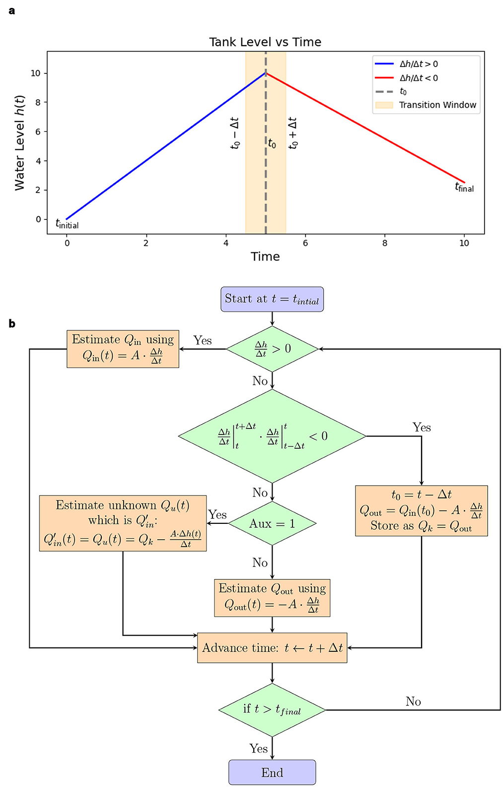
Figure 3. (a) A sample tank level trajectory with the characteristic slope changes, transition window. (b) Flow chart of algorithm.

By integrating level changes and auxiliary data within this dynamic framework, the monitoring system becomes adaptive to real-world variability. It allows robust estimation even during simultaneous flows, supports scalable deployment without needing complete sensorization, and improves the accuracy of water usage measurement over long-term operations. Although this dynamic approach works reliably in practice, it is important to theoretically quantify the estimation error incurred due to flow variability and finite observation windows. We now present a formal derivation of the error bounds under mild regularity assumptions.

2.4.2.1 Theoretical justification for dynamic estimation accuracy

In practical water systems, flow rates such as Q_in(t) and Q_out(t) fluctuate over time due to changing demands, supply variations, and operational factors, as discussed earlier. In order to estimate unknown flows in the presence of fluctuations, our dynamic estimation method assumes that during each estimation window, the known flow Q_k remains approximately constant, and that the flow rates are Lipschitz continuous, i.e., there is a limit on rate of change of the flow rates.

To rigorously quantify the impact of these assumptions on the estimation accuracy, we now derive a formal error bound. We show that:

• The estimation error introduced by the dynamic method remains small and controlled, provided the known and unknown flows do not change too rapidly.

• The additional error from using a previously estimated constant Q_k (from a nearby isolated flow period) also remains bounded and manageable.

The following proof establishes that the total estimation error grows linearly with the time window size Δt and the delay τ from the isolated transition time t₀, and is fully controlled by the Lipschitz constants of the flows.

Assumptions : Both Q_k(t) and Q_u(t) are assumed to be Lipschitz continuous with constants L_k and L_u, respectively. Further, we assume that Q_k is an outlet.

$|Q_i(t_1)-Q_i(t_2)|\le L_i|t_1-t_2|\text{\hspace{1em}for all }{t}_1,t_2\text{ and }i\in \{k,u\}.$

Mass balance : Over the interval [t, t+Δt], the mass balance gives:

${\displaystyle {\int }_t^{t+\Delta t}[}{Q}_k(s)-Q_u(s)]ds=s_k·A[h(t+\Delta t)-h(t)].$

Dynamic estimator : We assume that Q_k at t = t₀ is known. Defining ${\hat{Q}}_k=Q_k(t_0)$, we approximate $Q_k(t)\approx {\hat{Q}}_k$. we estimate ${\hat{Q}}_u(t)$ as follows:

${\hat{Q}}_u(t)=s_k·\frac{A\left[h(t+\Delta t)-h(t)\right]}{\Delta t}+{\hat{Q}}_k.$

Error decomposition : Assume Q_k is an outlet. By mass balance:

$-A[h(t+\Delta t)-h(t)]={\displaystyle {\int }_t^{t+\Delta t}[}{Q}_k(s)-Q_u(s)]ds.$

Dividing both sides by Δt and rearranging terms:

${\hat{Q}}_u(t)={\hat{Q}}_k-\frac{1}{\Delta t}{\displaystyle {\int }_t^{t+\Delta t}}\left[Q_k(s)-Q_u(s)\right]ds.$

Add and subtract Q_u(t) and Q_k(t):

$\begin{array}{r}{\hat{Q}}_u(t)-Q_u(t)=\left[{\hat{Q}}_k-Q_k(t)\right]+\left[Q_k(t)-\frac{1}{\Delta t}{\displaystyle {\int }_t^{t+\Delta t}}{Q}_k(s)ds\right]\\ +\left[\frac{1}{\Delta t}{\displaystyle {\int }_t^{t+\Delta t}}(Q_u(s)-Q_u(t))ds\right].\end{array}$

After rearranging terms:

$\begin{array}{r}{\hat{Q}}_u(t)-Q_u(t)=\left[{\hat{Q}}_k-Q_k(t)\right]+\left[\frac{1}{\Delta t}{\displaystyle {\int }_t^{t+\Delta t}}(Q_k(t)-Q_k(s))ds\right]\\ +\left[\frac{1}{\Delta t}{\displaystyle {\int }_t^{t+\Delta t}}(Q_u(s)ds-Q_u(t))\right].\end{array}$

From the triangle inequality, we have

$\begin{array}{r}|{\hat{Q}}_u(t)-Q_u(t)|\le |{\hat{Q}}_k-Q_k(t)|+\left|\frac{1}{\Delta t}{\displaystyle {\int }_t^{t+\Delta t}}(Q_k(t)-Q_k(s))ds\right|\\ +\left|\frac{1}{\Delta t}{\displaystyle {\int }_t^{t+\Delta t}}(Q_u(s)-Q_u(t))ds\right|.\end{array}$

Each term can be bounded separately using Lipschitz continuity. Applying the generalized triangle inequality and using the fact that Q_i is L_i-Lipschitz, i.e., |Q_i(t)−Q_i(s)| ≤ L_i|t−s|. we have:

$\begin{array}{r}\left|\frac{1}{\Delta t}{\displaystyle {\int }_t^{t+\Delta t}}(Q_i(t)-Q_i(s))ds\right|\le \frac{1}{\Delta t}{\displaystyle {\int }_t^{t+\Delta t}}|(Q_i(t)-Q_i(s))|\\ ds\le \frac{L_i}{\Delta t}{\displaystyle {\int }_t^{t+\Delta t}}|t-s|ds.\end{array}$

Over the interval [t, t+Δt], we have s≥t, so:

${\displaystyle {\int }_t^{t+\Delta t}}|t-s|ds={\displaystyle {\int }_t^{t+\Delta t}}(s-t)ds.=\frac{\Delta t^2}{2}$

Thus:

$\frac{1}{\Delta t}{\displaystyle {\int }_t^{t+\Delta t}}|(Q_i(t)-Q_i(s))|ds\le \frac{L_i\Delta t}{2}.$

• If the known flow value Q_k is taken from a past transition time t₀, then using its Lipschitz continuity with constant L_k, we have:

$|{\hat{Q}}_k-Q_k(t)|\le L_k·|t-t_0|=L_k·\tau .$

• The averaging error due to the variation of Q_k(t) over the interval [t, t+Δt] is bounded by:

$\frac{1}{\Delta t}{\displaystyle {\int }_t^{t+\Delta t}}|(Q_k(t)-Q_k(s))|ds\le \frac{L_k\Delta t}{2}.$

• Similarly, for the unknown flow Q_u(t) with Lipschitz constant L_u, the averaging error is:

$\frac{1}{\Delta t}{\displaystyle {\int }_t^{t+\Delta t}}|Q_u(s)-Q_u(t)|ds\le \frac{L_u\Delta t}{2}.$

Total error bound : Adding these bounds together yields the total estimation error:

$\begin{array}{||}\hline \left|{\widehat{Q}}_u(t)-Q_u(t)\right|\le L_k·\tau +\frac{L_k+L_u}{2}·\Delta t\\ \hline\end{array}$

This expression shows that the dynamic estimation remains accurate as long as:

• The known flow Q_k(t) is slowly varying (L_k is small),

• The unknown flow Q_u(t) is also smooth (L_u is small),

• The estimation window Δt and delay τ from the transition time are small.

Thus, under mild Lipschitz continuity assumptions, the dynamic flow estimation method guarantees that the error between the estimated and true unknown flow is bounded by a term proportional to the time window size Δt and the delay τ from the transition point. By choosing small enough Δt and ensuring Q_k is as close to the transition, an accurate and stable flow estimation is achieved even without simultaneous direct measurement of both flows.

3 Results

3.1 Case study 1

This case study is a controlled laboratory experiment, as shown in Figure 4. A 100-liter OHT, which is fed by a centrifugal pump of 0.5 HP capacity, pumping water from the ground-based reservoir of 650 L capacity. The system includes control mechanisms, such as Data Acquisition (DAQ) modules to regulate the on/off state of the pump and a continuously adjustable control valve for the outlet. The automatic logging of these switching events through LabVIEW provides valuable auxiliary data. To accurately measure the water flow, Keyence FD-Q10C and Keyence FD-Q20C were installed at the outlet and inlet pipes, respectively, while the HC-SR04 ultrasonic sensor was used as a level sensor.

Figure 4

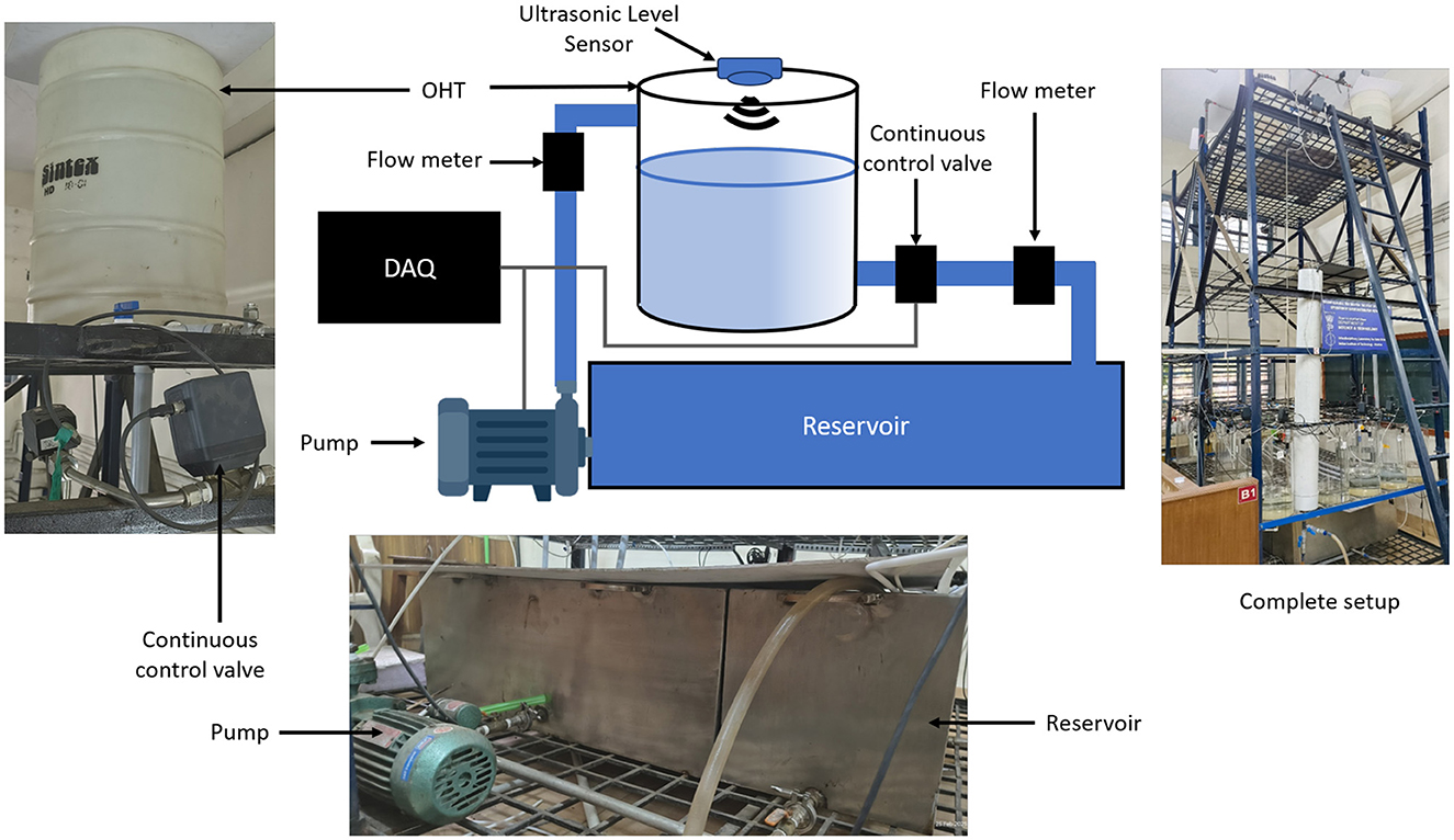
Figure 4. Experimental setup.

3.1.1 Baseline experiment

A series of initial experiments were conducted to determine the inlet flow rate Q_in and outlet flow rate Q_out under controlled conditions. The Q_in was maintained constant, as the water was pumped from a reservoir with a stable water supply. To characterize the outlet flow, the control valve at the tank outlet was adjusted to two distinct states: a fully open condition, where the valve allowed unrestricted flow, and a half-open condition, where the valve was partially closed to restrict outflow. Figures 5a, b illustrates the tank level profiles for various experimental combinations, while Table 1 presents the flow rates corresponding to the marked sections in the baseline experiments. In the same Figure, the horizontal flat lines are when both inlet and outlet are off. These predefined flow rates serve as reference values for the method discussed in Section 2.4.1, where known flow rates and auxiliary data are used. Notably, since the valve adjustments were controlled, the timestamps of actuation events themselves serve as auxiliary data for analysis.

Figure 5

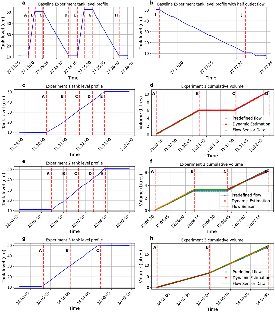
Figure 5. (a, b) Tank level profiles for baseline experiments, with corresponding sections marked as detailed in Table 1 while (c, e, g) are the tank level profiles for the experiments done for validation and (d, f, h) are the comparison of estimated cumulative volume with the flow sensor data for the validation experiments. This is summarized in the Table 2.

Table 1

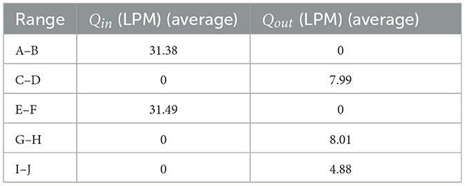
Table 1. Flow rates corresponding to the marked sections in the baseline experiments, as illustrated in Figures 5a, b.

3.1.2 Validation of flow estimation methods

Building upon the baseline experiments, three additional tests were conducted in which both the inlet and outlet flows were active simultaneously. During these experiments, the inlet valve remained open, while the outlet valve was adjusted to either fully open or half-open at different intervals to create varying flow conditions. Figures 5c, e, g present the tank level profiles for experiments 1, 2, and 3, respectively, with the corresponding flow condition sections detailed in Table 2.

• Experiment 1: The inlet valve was open throughout. The outlet valve was fully open at different intervals.

• Experiment 2: The inlet valve was open throughout. The outlet valve was half-open at different intervals.

• Experiment 3: The inlet valve was open throughout. The outlet valve was initially half-open and then switched to fully open.

Table 2

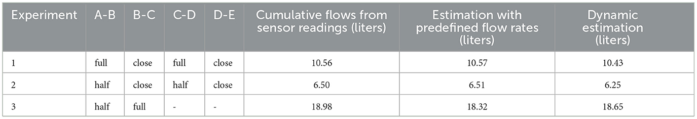
Table 2. Outlet valve conditions for the marked sections in Figures 5c, e, g and final cumulative volume values for Experiments 1, 2, and 3 corresponding to the plots in Figures 5d, f, h.

The actual timestamps of valve operations were recorded, providing precise data on flow variations. These experiments enable testing the estimation approach under dynamic inlet and outlet conditions, aiding in the validation of the proposed method's reliability in real-world applications. In the experiments conducted, the flows were recorded via a flow sensor for validation. The method described in Section 2.4.1, which utilizes predefined flow rates along with auxiliary data, was initially applied to estimate water consumption. Our primary focus is on estimating the Q_out(t) at any given time, as it is the lesser of the two (inlet and outlet) and also varies, which is challenging to estimate while the inlet flow remains constant throughout the experiment. Therefore, the estimation is performed on the outlet flow, and the results are validated using the flow sensor measurements.

The cumulative volumes for the three experiments are plotted in Figures 5d, f, h where both the methods and the flow sensor data are overlapping throughout the experiments. The final values obtained are presented in Table 2. The results demonstrate that the estimated cumulative volumes using predefined flow rates closely matched the actual recorded values from the flow sensor, with minimal error. For Experiment 1, the predefined method estimated 10.57 liters, closely matching the sensor reading of 10.56 liters. Similarly, for Experiment 2, the predefined method yielded 6.51 liters, compared to the sensor reading of 6.50 liters. However, in Experiment 3, the predefined method resulted in 18.32 liters, which had a slightly higher deviation from the sensor measurement of 18.98 liters.

Subsequently, the method discussed in Section 2.4.2, which dynamically estimates flow rates based on the observed level changes and historical trends, was applied to the same experiments where Q_k is the inlet flow rate as it is constant throughout the experiment, while Q_u is the outlet flow rate which changes throughout the experiment and can be determined using Equation 7. The cumulative volume is plotted in the same figures, with final values of 10.43 liters, 6.25 liters, and 18.65 liters for Experiments 1, 2, and 3, respectively. The results show a slightly higher error compared to the predefined flow method in Experiments 1 and 2. However, in Experiment 3, the dynamic method performed better than the predefined method, yielding an estimate (18.65 liters) that was closer to the actual value (18.98 liters). This improvement in accuracy for Experiment 3 can be attributed to the fact that the outlet flow condition changed mid-experiment–from half-open to fully open. Unlike predefined flow estimation, which assumes constant flow rates based on historical data, the dynamic method adjusts based on observed level changes. Since the predefined method assumes a single flow rate per valve position, it could not fully capture the transition between half-open and fully open conditions in Experiment 3, leading to a greater deviation. In contrast, the dynamic approach was able to detect this variation and adjust accordingly, resulting in a more accurate cumulative volume estimate. Despite slightly higher errors in Experiments 1 and 2, the dynamic approach demonstrated its potential advantage when flow conditions change within the estimation period, making it a more suitable method in scenarios where predefined flow rates may not fully capture transient flow behavior.

3.2 Case study 2

This case study was conducted on an overhead tank with a capacity of 30,000 liters, which supplies water to a peri-urban area in Chennai, India. The inlet source is a borewell, presenting a key challenge, that is the yield is not constant throughout the year. Additionally, the outlet connects to a distribution network, where withdrawal rates vary significantly based on the time of day. To monitor and analyze the system, pump operation data was recorded and transmitted to the cloud storage. Pump status information is obtained from the electrical contactors in the pump circuit. The baseline experiments revealed that the inlet flow rate from the pump was the lowest. Therefore, auxiliary data should be obtained from the inlet side, and in this case, the pump status is the auxiliary signal. The setup is shown in Figure 6 where, in addition to the level sensor, a flow meter was installed at the inlet to validate the methodology.

Figure 6

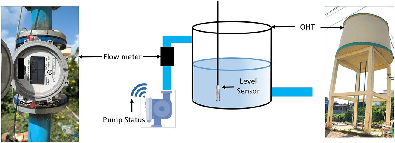
Figure 6. Illustration of the setup, including the overhead tank and meter installation.

3.2.1 Baseline experiment

To conduct baseline experiments and determine the lower flow rate between the inlet and outlet, each was opened sequentially. Table 3 presents the marked sections of average flow rates in liters per minute (LPM) from the baseline experiment, as illustrated in Figure 7. It is clear that the borewell flow rate is lower than the tank outlet flow rate. The flow meter readings were recorded every 5 min, and both the cumulative volume and inlet flow rate are plotted in Figures 7b, c. One of the key challenges in this system is the gradual decline and fluctuation in borewell yield over time, which is evident in the same figure, combined with the intermittent nature of the outlet flow, which varies depending on the time of day when water is distributed to the community.

Table 3

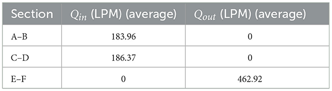
Table 3. Average flow rate for the sections corresponding to the tank level profiles shown in Figure 7a.

Figure 7

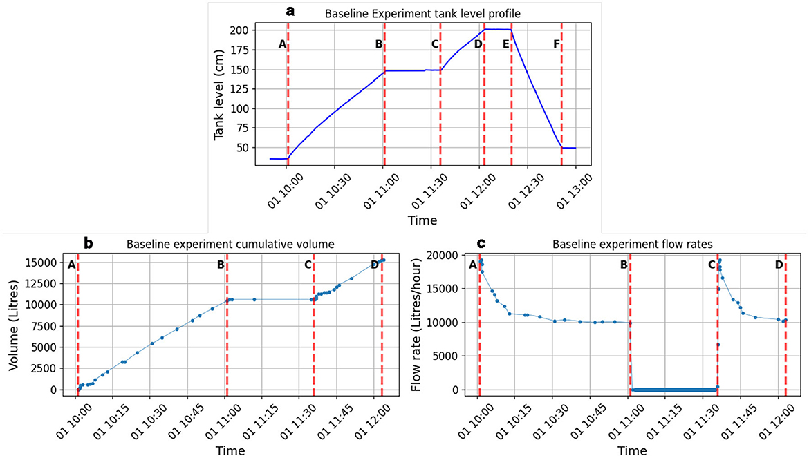
Figure 7. (a) tank level profiles from the baseline experiment, with corresponding sections marked as detailed in Table 3. (b, c) inlet cumulative volume and the inlet flow rates for the baseline experiment respectively.

3.2.2 Validation of flow estimation methods

The dataset for this analysis spans over 13 days. To validate the proposed methods, totalized volume readings from a flow meter were recorded at different points in time, with at least a day between consecutive readings. This approach ensured that cumulative errors could be observed and analyzed over an extended period. Unlike the controlled baseline experiments, this scenario was entirely uncontrolled, meaning the operator turned the pump on and off as needed to meet the requirements of the distribution network. Figure 8 illustrates the tank level profile along with the corresponding pump status over the observed period. The pump status is represented as 1 whenever the pump is turned on and 0 when it is off, providing a clear indication of active pumping intervals and their impact on tank level fluctuations. The challenge in such an uncontrolled setting is that the operator's actions, network withdrawal rates, and pump operation schedules vary dynamically. Both estimation methods were evaluated to assess their accuracy in determining water consumption. The predefined flow rate method, derived from baseline experiments, was applied whenever the pump status was on. This approach assumes that the borewell yield remains constant throughout the experiment, similar to the methodology used in Case Study 1 (Section 3.1). Alternatively, the dynamic flow estimation method was implemented, where flow rates were continuously adjusted based on tank level changes.

Figure 8

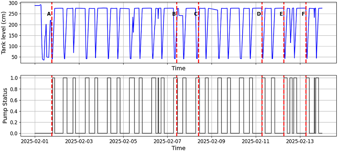
Figure 8. Tank level profile and corresponding pump status over the observed period.

The dynamic estimation allows for adaptation to changing conditions without assuming a constant borewell flow rate over the entire period. This algorithm is applied only to the time intervals when the pump is active within the given dataset. For the dataset presented in Figure 8, the marked section indicates the recorded cumulative values at specific timestamps. Table 4 provides a comparison of volume estimations obtained using both the predefined flow rate method and the dynamic flow estimation method, alongside the actual recorded values from the flow meter.

Table 4

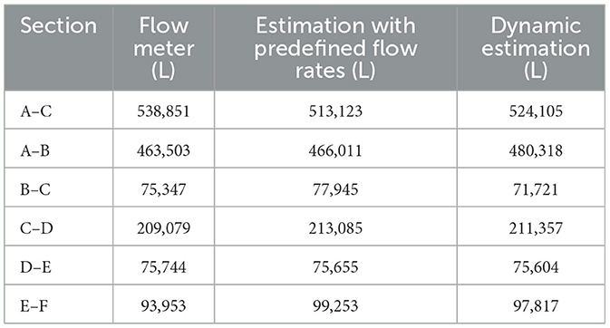
Table 4. Comparison of volume estimations using predefined flow rate and dynamic flow estimation methods with actual recorded values from the flow meter.

As discussed earlier, the predefined flow rate method relies on flow rates recorded during baseline experiments. However, in real-world scenarios, this assumption is rarely accurate. Bore well flow rates fluctuate over time due to groundwater depletion and seasonal variations, leading to potential errors when applying a fixed flow rate over extended periods. The estimation error is likely to increase as seasonal conditions change. Additionally, this method requires prior knowledge of the flow rate, which may not always be available. The predefined method yielded a mean absolute percentage error (MAPE) of 2.73%, with a 95% confidence interval ranging from 1.18% to 4.40%. While, dynamic flow estimation approach continuously adjusts flow rates based on tank level changes, allowing for better adaptability to fluctuations in bore well yield and network withdrawal patterns. However, despite its flexibility, the dynamic method resulted in a slightly higher MAPE of 2.76%, with a 95% confidence interval ranging from 1.42% to 4.00%.

This approach was further extended to two additional 30,000-liter OHTs within the same peri-urban region of Chennai, where similar water distribution patterns were observed. While no dedicated flow meters were installed at these sites, the methodology was still applied using tank level sensors and auxiliary data. Figure 9 illustrates the tank level profiles for two additional OHTs along with the daily water supply estimation using the dynamic estimation method, highlighting the daily supply patterns. These profiles provide valuable insights into the system's operational characteristics, including refilling schedules, withdrawal trends, and supply intermittency. The results demonstrate that the proposed method remains effective even in real-world scenarios where direct flow measurement is unavailable, reinforcing its potential for scalable deployment in similar water distribution systems.

Figure 9

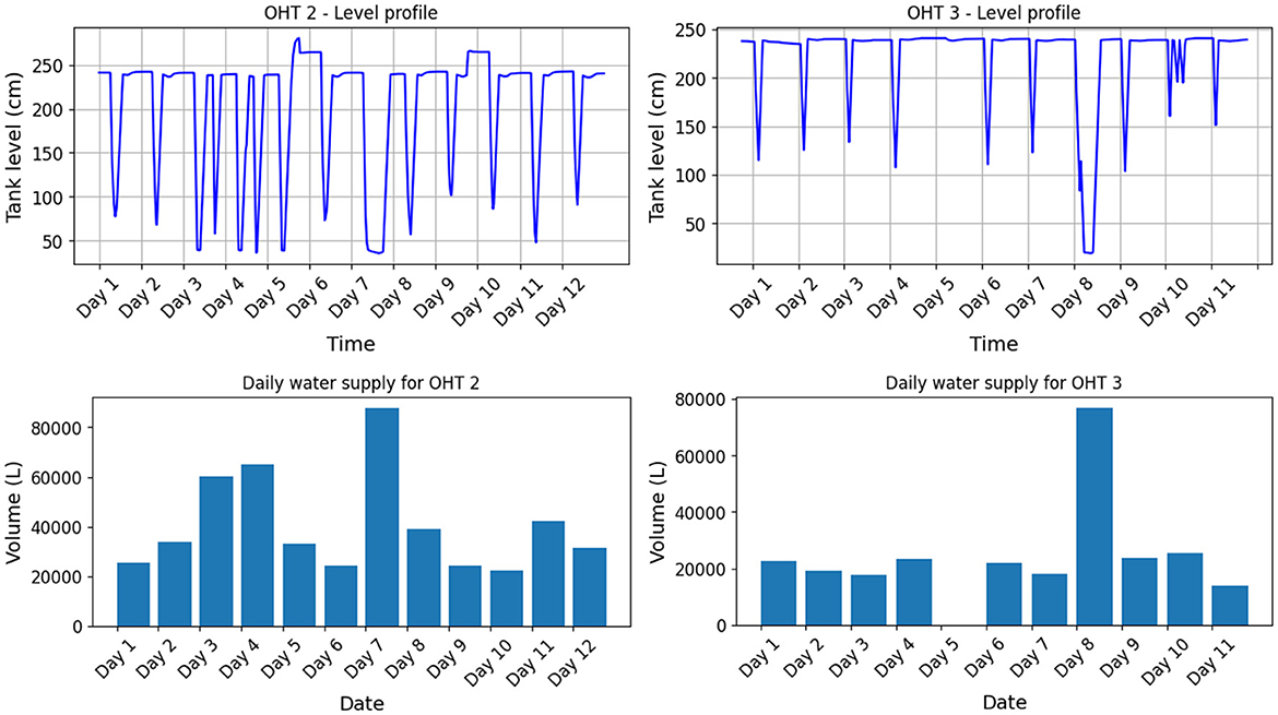
Figure 9. Tank level profile with the corresponding daily water supply.

3.3 Case study 3

Building on the approach outlined in Case Study 2, this methodology was validated with another system operating within the IIT Madras campus. The setup used is identical to that described in Raphael and Narasimhan (2022), where the estimation is performed on a sump system. In this setup, the YF-DN50 flow sensor is installed on the outlet side of the sump, and the MB7566 SCXL-MaxSonar-WR ultrasonic sensor is used to measure the level of water in the sump.

The tank level profiles illustrated in Figure 2 are used for estimating inlet and outlet flows. This system presents unique challenges as the outlet flow rate changes abruptly when demand is met at the demand node, and the inlet flow rate shows significant variations. In such complex systems, relying on predefined flow rates is impractical. Therefore, in this case study, auxiliary data is utilized by identifying timestamps when the outlet flow rate is greater than zero.

The figure shows that initially there are periods where the outlet is active, but the sump level remains flat, followed by an increase when the outlet is turned off. This indicates that the inlet was also active during this time, making the inlet and outlet flow rates equal. In this scenario, the Q_out which is an unknown flow rate Q_u was estimated using Equation 7 by considering Q_in from the nearest increasing period. Finally, when only the outlet is active, the sump level decreases. The final volume obtained for outlet volume from the flow sensor is 16,553 liters, and through dynamic estimation it is 17,113 liters.

4 Discussion and conclusion

This study presented a cost-effective and non-intrusive approach to estimating water consumption in overhead tanks (OHTs) and reservoirs by utilizing tank level sensors and auxiliary data sources. Unlike conventional smart meters, which require intrusive installation and are expensive, our methodology provides a scalable alternative that significantly reduces infrastructure and operational costs while maintaining high accuracy.

Two estimation methods were explored: predefined flow rate estimation and dynamic flow estimation. The predefined flow method relied on flow rates obtained from baseline experiments and auxiliary indicators such as pump status, demonstrating minimal error when flow rates remained stable. However, due to the natural variability of the borewell yields and fluctuating demand patterns, this approach can introduce higher errors over extended periods. To address this, the dynamic flow estimation method was implemented, which continuously updates flow rates based on tank level variations. This method proved to be more adaptive, effectively capturing short-term fluctuations in borewell yield and network withdrawal.

While the dynamic method relies on physical principles and trend filtering, its structure aligns closely with implicit regularization objectives commonly seen in machine learning. This opens up future opportunities to treat flow estimation as a learning problem, where data-driven methods could complement the physics-based models to improve robustness. This interpretation opens the door to incorporating additional learning-based extensions, such as adaptive regularization, Bayesian priors, or neural approximators for flow patterns under more complex settings.

The proposed approach was validated through controlled and uncontrolled case studies, demonstrating its robustness across various operational conditions. The results indicate that while predefined flow rates provide highly accurate estimations under controlled settings, dynamic flow estimation is better suited for real-world scenarios where flow rates are subject to change.

In terms of affordability, Commercial Off-The-Shelf (COTS) 3-inch smart water meters, typically used in 30,000-liter OHTs, with built-in communication capabilities that periodically store data in the cloud are available. These meters cost approximately $500, with an additional $250 for installation. While they can be used upto a maximum flow rate of 100,000 liters per hour, they are often optimized for a limited operational range and can struggle with accuracy at lower flow rates also their accuracy deteriorates over time due to factors such as silt deposition and pipeline corrosion. Offsite recalibration requires the instrument to be removed and serviced while onsite recalibration requires experienced technicians and portable reference equipment. In contrast, the methodology proposed in this paper provides a cost-effective alternative, with total expenses–including installation–limited to approximately $75, without limiting the range of flow rate, while maintaining reliable water usage monitoring. Moreover, it simplifies commissioning, requiring no invasive plumbing modifications or specialized equipment. Calibration is straightforward and does not require mobile calibrators or specialized technicians and does not rely on fixed flow measurement ranges, allowing it to adapt seamlessly across a wide range of flow conditions.

This approach directly supports Sustainable Development Goal 6, particularly Target 6.5, which calls for implementing integrated water resources management at all levels (United Nations, n.d.). By enabling flow estimation without intrusive infrastructure, the method equips utilities with actionable data to balance supply and demand, reduce losses, and improve decision-making. It complements initiatives such as India's Jal Jeevan Mission (Ministry of Jal Shakti, 2022, 2019), which emphasizes on robust operation and maintenance, community-led monitoring, and data-driven decision making. Moreover, by equipping local governance bodies with analytical tools that do not rely on high-cost flow meters, the approach promotes transparency, empowers low-level committees, and supports sustainable service delivery. The insights gained from such analysis can also inform national-level policy and planning by identifying systemic issues and prioritizing infrastructure interventions.

In conclusion, this study establishes a reliable, smart water metering framework that requires minimal infrastructure. The proposed approach offers a practical, scalable solution for water management, particularly in resource-constrained environments, paving the way for more efficient and sustainable water distribution systems. The proposed methodologies are filed under Indian Patent CONFIDENTIAL; - PATENT PENDING 202541010251.

Data availability statement

The original contributions presented in the study are included in the article/Supplementary material, further inquiries can be directed to the corresponding author.

Author contributions

MJ: Formal analysis, Investigation, Methodology, Software, Writing – original draft. RR: Formal analysis, Investigation, Methodology, Software, Writing – review & editing. SR: Investigation, Writing – review & editing. HB: Investigation, Writing – review & editing. SN: Writing – review & editing, Conceptualization, Funding acquisition, Supervision.

Funding

The author(s) declare that financial support was received for the research and/or publication of this article. This work was supported by AquaMAP, IIT Madras (grant number: SB21221878CHDONO008328) and the Robert Bosch Centre for Data Science and Artificial Intelligence (RBCDSAI), IIT Madras (grant number: CR1920CH1061RBCX008328).

Conflict of interest

The authors declare that the research was conducted in the absence of any commercial or financial relationships that could be construed as a potential conflict of interest.

Generative AI statement

The author(s) declare that Gen AI was used in the creation of this manuscript. To help write the manuscript ChatGPT-4o is used.

Publisher's note

All claims expressed in this article are solely those of the authors and do not necessarily represent those of their affiliated organizations, or those of the publisher, the editors and the reviewers. Any product that may be evaluated in this article, or claim that may be made by its manufacturer, is not guaranteed or endorsed by the publisher.

Supplementary material

The Supplementary Material for this article can be found online at: https://www.frontiersin.org/articles/10.3389/frwa.2025.1586916/full#supplementary-material

References

Abu-Bakar, H., Williams, L., and Hallett, S. H. (2021). A review of household water demand management and consumption measurement. J. Clean. Prod. 292:125872. doi: 10.1016/j.jclepro.2021.125872

PubMed Abstract | Crossref Full Text | Google Scholar

American Water Works Association (2020). AWWA C700-20 Cold-Water Meters-Displacement Type, Bronze Main Case. Available online at: https://www.amwater.com/corp/resources/pdf/military-services/33-12-33-Water-Meters.pdf (accessed April 25, 2025).

Google Scholar

Bureau of Indian Standards (1994). IS 779:1994 Water Meters (Domestic Type) – Specification. Available online at: https://law.resource.org/pub/in/bis/S03/is.779.1994.pdf (accessed April 25, 2025).

Google Scholar

Campbell, T., Larson, E., Cohn, G., Froehlich, J., Alcaide, R., and Patel, S. N. (2010). “WATTR: a method for self-powered wireless sensing of water activity in the home,” in Proceedings of the 12th ACM International Conference on Ubiquitous Computing, UbiComp '10 (New York, NY: Association for Computing Machinery), 169–172.

Google Scholar

Cassiolato, G. H., Ruiz-Femenia, J. R., Salcedo-Diaz, R., and Ravagnani, M. A. (2024). Water distribution networks optimization considering uncertainties in the demand nodes. Water Resour. Managem. 38, 1479–1495. doi: 10.1007/s11269-024-03733-y

Crossref Full Text | Google Scholar

Cherqui, F., James, R., Poelsma, P., Burns, M. J., Szota, C., Fletcher, T., et al. (2020). A platform and protocol to standardise the test and selection low-cost sensors for water level monitoring. H2Open J. 3, 437–456. doi: 10.2166/h2oj.2020.050

Crossref Full Text | Google Scholar

Chinnusamy, S., Mohandoss, P., Kurian, V., Narasimhan, S., and Narasimhan, S. (2018a). “Operation of intermittent water distribution systems: an experimental study,” in 13th International Symposium on Process Systems Engineering (PSE 2018), eds. M. R. Eden, M. G. Ierapetritou, and G. P. Towler (London: Elsevier).

Google Scholar

Chinnusamy, S., Mohandoss, P., Paul, P., Murali, N., Bhallamudi, S. M., Narasimhan, S., et al. (2018b). “IoT enabled monitoring and control of water distribution network,” in WDSA/CCWI Joint Conference 2018 (Kingston, ON: Queen's University Library's Journal Hosting Platform, Open Journal Systems).

PubMed Abstract | Google Scholar

Choudhary A. K. and Singh, V.. (2024). Investigating the changing pattern of groundwater levels and rainfall in the peninsular region of Bhagalpur and Khagaria, Bihar. Water Supply 24, 465–479. doi: 10.2166/ws.2024.010

Crossref Full Text | Google Scholar

DFRobot (n.d.). Sku:kit0139. Available online at: https://wiki.dfrobot.com/Throw-in_Type_Liquid_Level_Transmitter_SKU_KIT0139 (accessed April 25, 2025).

Google Scholar

Ding, N., Zhu, Q., Cherqui, F., Walcker, N., Bertrand-Krajewski, J.-L., and Hamel, P. (2025). Laboratory performance assessment of low-cost water level sensor for field monitoring in the tropics. Water Res. X 27:100298. doi: 10.1016/j.wroa.2024.100298

PubMed Abstract | Crossref Full Text | Google Scholar

Froehlich, J. E., Larson, E., Campbell, T., Haggerty, C., Fogarty, J., and Patel, S. N. (2009). “Hydrosense: infrastructure-mediated single-point sensing of whole-home water activity,” in Proceedings of the 11th International Conference on Ubiquitous Computing, UbiComp '09 (New York, NY: Association for Computing Machinery), 235–244.

Google Scholar

Hejazi, M., Silva, S. R. S. D., Miralles-Wilhelm, F., Kim, S., Kyle, P., Liu, Y., et al. (2023). Impacts of water scarcity on agricultural production and electricity generation in the middle east and north africa. Front. Environm. Sci. 11:1082930. doi: 10.3389/fenvs.2023.1082930

Crossref Full Text | Google Scholar

Indian Infrastructure (2023). Water Losses: Nrw Impact and Reduction Initiatives. Available online at: https://indianinfrastructure.com/2023/05/29/water-losses-nrw-impact-and-reduction-initiatives/ (accessed Februaury 02, 2025).

Google Scholar

International Organization for Standardization (2014). ISO 4064:2014 Water Meters for Cold Potable Water and Hot Water-Part 1: Metrological and Technical Requirements. Available online at: https://cdn.standards.iteh.ai/samples/55386/c15a0f8cd91844c7b2538cf44913bd1f/ISO-4064-5-2014.pdf (accessed April 25, 2025).

Google Scholar

Ismail, M. I. M., Dziyauddin, R. A., and Samad, N. A. A. (2014). “Water pipeline monitoring system using vibration sensor,” in 2014 IEEE Conference on Wireless Sensors (ICWiSE) (Subang: IEEE), 79–84.

Google Scholar

Kim, S.-J., Koh, K., Boyd, S., and Gorinevsky, D. (2009). ℓ₁ trend filtering. SIAM Rev. 51, 339–360. doi: 10.1137/070690274

Crossref Full Text | Google Scholar

Kim, Y., Schmid, T., Charbiwala, Z. M., Friedman, J., and Srivastava, M. B. (2008). “NAWMS: nonintrusive autonomous water monitoring system,” in Proceedings of the 6th ACM Conference on Embedded Network Sensor Systems, SenSys '08 (New York, NY: Association for Computing Machinery), 309–322.

Google Scholar

Kurian, V., Mohandoss, P., Chandrakesa, S., Chinnusamy, S., Narasimhan, S., and Narasimhan, S. (2023). Equitable supply in intermittently operated rural water networks in emerging economies. Water Supply 23, 4520–4538. doi: 10.2166/ws.2023.268

Crossref Full Text | Google Scholar

Madias, K., Borusiak, B., and Szymkowiak, A. (2022). The role of knowledge about water consumption in the context of intentions to use IoT water metrics. Front. Environm. Sci. 10:934965. doi: 10.3389/fenvs.2022.934965

Crossref Full Text | Google Scholar

Madias, K., Szymkowiak, A., and Borusiak, B. (2023). What builds consumer intention to use smart water meters – extended TAM-based explanation. Water Res. Econ. 44:100233. doi: 10.1016/j.wre.2023.100233

Crossref Full Text | Google Scholar

MathWorks (n.d.a). ThingSpeak – MATLAB & Simulink. Available online at: https://in.mathworks.com/products/thingspeak.html (accessed May 6, 2025).

PubMed Abstract | Google Scholar

MathWorks (n.d.b). Channel Data Control – MATLAB & Simulink. Available online at: https://in.mathworks.com/help/thingspeak/channel-control.html (accessed May 6, 2025).

Google Scholar

Minea, I., Boicu, D., Amihăiesei, V., and Iosub, M. (2022). Identification of seasonal and annual groundwater level trends in temperate climatic conditions. Front. Environm. Sci. 10:2022. doi: 10.3389/fenvs.2022.852695

Crossref Full Text | Google Scholar

Ministry of Jal Shakti (2019). Operational Guidelines, Jal Jeevan Mission (Har Ghar Jal). Available online at: https://jaljeevanmission.gov.in/sites/default/files/guideline/JJM_Operational_Guidelines.pdf (accessed April 25, 2025).

Google Scholar

Ministry of Jal Shakti (2022). Reforms in Rural Drinking Water Supply - jal Jeevan Mission (Har Ghar Jal). Available online at: https://jaljeevanmission.gov.in/sites/default/files/guideline/JJM-Reform-Document-English.pdf (accessed April 25, 2025).

Google Scholar

Ministry of Jal Shakti (2024). Per Capita Water Availability. Available online at: https://pib.gov.in/PressReleaseIframePage.aspx?PRID=2002726 (accessed Februaury 25, 2025).

Google Scholar

Mohindru, P. (2023). Development of liquid level measurement technology: a review. Flow Measurem. Instrument. 89:102295. doi: 10.1016/j.flowmeasinst.2022.102295

Crossref Full Text | Google Scholar

Raphael R. and Narasimhan, S.. (2022). “Data driven monitoring of IOT enabled water distribution networks,” in 2nd WDSA/CCWI Joint Conference (Valencia: Universitat Politècnica de València (Valencia Tech)), 18–22.

PubMed Abstract | Google Scholar

Raphael, R., Prasath Ramprasad, S. H., and Narasimhan, S. (2024). Cloud-based control and monitoring of water distribution network using free spectrum communication protocols. Eng. Proc. 69:1. doi: 10.3390/engproc2024069071

Crossref Full Text | Google Scholar

Richard Koech R. C.-O. and Syme, G.. (2021). Smart water metering: adoption, regulatory and social considerations. Aust. J. Water Res. 25, 173–182. doi: 10.1080/13241583.2021.1983968

Crossref Full Text | Google Scholar

Sankar, G. S., Mohan Kumar, S., Narasimhan, S., Narasimhan, S., and Murty Bhallamudi, S. (2015). Optimal control of water distribution networks with storage facilities. J. Process Control, 32, 127–137. doi: 10.1016/j.jprocont.2015.04.007

Crossref Full Text | Google Scholar

Shamsudduha, M., Chandler, R. E., Taylor, R. G., and Ahmed, K. M. U. (2009). Recent trends in groundwater levels in a highly seasonal hydrological system: the Ganges-Brahmaputra-Meghna Delta. Hydrol. Earth Syst. Sci. 13, 2373–2385. doi: 10.5194/hess-13-2373-2009

Crossref Full Text | Google Scholar

Spedaletti, S., Rossi, M., Comodi, G., Cioccolanti, L., Salvi, D., and Lorenzetti, M. (2022). Improvement of the energy efficiency in water systems through water losses reduction using the district metered area (DMA) approach. Sustain. Cities Soc. 77:103525. doi: 10.1016/j.scs.2021.103525

Crossref Full Text | Google Scholar

Suresh, M., Muthukumar, U., and Chandapillai, J. (2017). “A novel smart water-meter based on IoT and smartphone app for city distribution management,” in 2017 IEEE Region 10 Symposium (TENSYMP) (Cochin: IEEE),1–5.

Google Scholar

Tibshirani, R. J. (2014). Adaptive piecewise polynomial estimation via trend filtering. Ann. Statist. 42:1. doi: 10.1214/13-AOS1189

Crossref Full Text | Google Scholar

Ullah, I., Zeng, X. M., Hina, S., Syed, S., Ma, X., Iyakaremye, V., et al. (2023). Recent and projected changes in water scarcity and unprecedented drought events over southern pakistan. Front. Earth Sci. 11:1113554. doi: 10.3389/feart.2023.1113554

Crossref Full Text | Google Scholar

United Nations (2022). SDG Report 2022. Available online at: https://unstats.un.org/sdgs/report/2022/Goal-06 (accessed Februaury 25, 2025).

Google Scholar

United Nations (n.d.). Goal 6: Clean Water and Sanitation - The Global Goals. Available online at: https://www.globalgoals.org/goals/6-clean-water-and-sanitation/ (accessed April 4, 2025).

Google Scholar

Vairavamoorthy, K., Gorantiwar, S. D., and Pathirana, A. (2008). Managing urban water supplies in developing countries – climate change and water scarcity scenarios. Phys. Chem. Earth 33, 330–339. doi: 10.1016/j.pce.2008.02.008

Crossref Full Text | Google Scholar

WMO (2021). Wake up to the Looming Water Crisis, Report Warns. Available online at: https://wmo.int/news/media-centre/wake-looming-water-crisis-report-warns (accessed Februaury 25, 2025).

Google Scholar

Zhou, X., Cheng, J., She, L., and Fan, G. (2020). Analysis of measuring characteristics of the differential pressure water-level measurement system under depressurization condition. Front. Energy Res. 8:555598. doi: 10.3389/fenrg.2020.00145

Crossref Full Text | Google Scholar