Overestimation of evapotranspiration across India if not considering the impact of rising atmospheric CO2

Evapotranspiration (ET), a key component of the hydrological cycle, responds to and influences climate change, making accurate estimation of reference ET (ET_o) critical for long-term impact assessments. The widely applied FAO Penman–Monteith (FAO-PM) equation for calculating ET_o does not account for rising atmospheric CO₂, which reduces vegetation stomatal conductance and can lead to systematic overestimation of ET_o. We derived a modified FAO-PM equation incorporating CO₂ effects on stomatal behavior. Using projections from five global circulation models, we compared spatiotemporal average of ET_o estimates for India from the original and modified equations under SSP5-8.5 and SSP1-2.6. Differences were 0.11–1.29 mm day⁻¹ (2021–2030), 0.09–1.90 mm day⁻¹ (2051–2060), and 0.17–3.14 mm day⁻¹ (2091–2100) under SSP5-8.5, with slightly lower values under SSP1-2.6. Seasonal differences between the predicted ET_o from the two equations peaked during the pre-monsoon, reaching 3.90 mm day⁻¹ (SSP5-8.5) and 1.74 mm day⁻¹ (SSP1-2.6). Neglecting stomatal responses to CO₂ could lead to ET_o overestimation of ~29% under SSP5-8.5 by 2100, potentially biasing projections of droughts, heatwaves, and water demand. By contrast, overestimation is moderate (~13%) under SSP1-2.6. Incorporating the impact of CO₂ into ET_o estimation is therefore essential for robust climate change impact assessments.

1 Introduction

The study of climate change and its effects on the hydrological cycle is a prominent and highly emphasized research field. Among the essential components of the hydrological cycle, evapotranspiration (ET) is one crucial component that is highly responsive to climate change and atmospheric CO₂ (Parasuraman et al., 2007; Abdolhosseini et al., 2012; Izady et al., 2013; Pan et al., 2015; Rezaei et al., 2016; Sarker, 2022). ET can affect discharge for a large-scale catchment (Dakhlaoui et al., 2020) and crop water requirements on a smaller scale (Djaman et al., 2018). Optimization of irrigation (Wright and Asae, 1985; Bashir et al., 2023) as a way for climate change adaptation (Li et al., 2020; Yang et al., 2023), also makes extensive use of ET estimations. ET can be estimated using field measurements (Tanner, 1967; Liu et al., 2013; Kompanizare et al., 2022) or modeling techniques (Wang et al., 2024). In contrast to field measurements (Tanner, 1967; Liu et al., 2013), modeling-based approaches (Allen et al., 1998; Das et al., 2023) to estimate ET are inexpensive because they rely on readily available meteorological data. One of the popular modeling-based approaches to estimate ET makes use of the FAO Penman-Monteith equation (FAO-PM) (Allen et al., 1998) to calculate reference evapotranspiration (ET_o) which is evapotranspiration for a hypothetical reference crop with an assumed crop height of 0.12 m, a fixed surface resistance of 70 s m⁻¹, and an albedo of 0.23 under well-watered condition. The ET_o is then multiplied by a crop specific parameter called crop coefficient (Allen et al., 1998) which varies by growth stages and management practices to determine the actual ET for a given crop. The fixed value of 70 s m⁻¹ of surface resistance, incorporated in the FAO-PM, is based on an assumption of a constant stomatal resistance of 100 s m⁻¹ for a single leaf (Allen et al., 1998). However, this assumption is not valid because increasing atmospheric CO₂ concentration is known to increase stomatal resistance (Ainsworth and Long, 2021). The global atmospheric CO₂ has increased from 320 ppm in 1965 (Statista, 2024), when the original Penman-Monteith equation (Monteith, 1965) was proposed, to 420 ppm in 2024, and CO₂ levels could potentially exceed 1,000 ppm by 2100 if the world follows the SSP5-8.5 pathway (Büchner and Reyer, 2022). Increasing CO₂ concentration by 300 ppm resulted in a 50% increase in stomatal resistance in a field study of grassland (Vremec et al., 2023). Ainsworth and Rogers (2007) reported a 28% increase in leaf-level stomatal resistance as CO₂ rose from 366 to 567 ppm across global bioclimates. Therefore, ET_o estimates made using the FAO-PM equation are prone to overestimation. This limitation has been addressed by incorporating a simple function into the FAO-PM equation that allows stomatal resistance to vary as a function of atmospheric CO₂ (Li et al., 2019; Yang et al., 2019). Incorporating the impact of CO₂ in calculating evapotranspiration (ET) led to a notable reduction in estimated water demand for maize grown under controlled condition (Li et al., 2019), and helped in addressing anomalies caused by the concurrent occurrence of drought conditions and increased runoff (Yang et al., 2019).

An accurate estimation of ET over contiguous India is crucial for the wellbeing of more than a billion people in the context of climate change. Several factors such as reliance on the 4 months of monsoon (Mall et al., 2006), intrinsic relationship between rainfall and ET (Stefanidis and Alexandridis, 2021), spatial–temporal mismatch between water demand and supply (Amarasinghe et al., 2007), makes it necessary to account for the impact of rising atmospheric CO₂ concentration in sustainable management of water resources in India. It is essential to consider rising atmospheric CO₂ in water resource planning. However, several studies focusing on the availability of water resources (Mall et al., 2006), agricultural water demand (Sreeshna et al., 2024), and extreme events such as flooding (Mall et al., 2006; Bharat and Mishra, 2021; Athira et al., 2023) and droughts (Aadhar and Mishra, 2020) often do not explicitly include the effect of rising CO₂ in their analyses. Earlier projections, which excluded the impact of CO₂, indicated a significant spatial and temporal variation in the increase in potential ET due to rising temperatures (Chattopadhyay and Hulme, 1997). In this study, we aim to investigate the influence of atmospheric CO₂ concentrations alongside future climate projections under SSP1-2.6 and SSP5-8.5 to reassess ET_o patterns across contiguous India. To achieve this, we modified the FAO-PM equation and utilized climate projections, including atmospheric CO₂ concentrations, to conduct a comprehensive analysis of the spatio-temporal variations in ET_o, both with and without accounting for the effects of rising CO₂ concentrations.

2 Methods

The overall methodology adopted in this study is summarized in the flowchart presented in Figure 1, which offers a step-by-step visual overview of the procedures and analyses undertaken to assess the impact of incorporating atmospheric CO₂ concentrations into the estimation of the reference evapotranspiration over India. Detailed explanations of each step are provided in the subsequent subsections. A key strength of this approach is the use of harmonized and bias-corrected future climate data (Hempel et al., 2013; Warszawski et al., 2014), which enables a consistent and spatially explicit evaluation of how excluding atmospheric CO₂ may influence evapotranspiration estimations in India, where water availability vary significantly over seasons and regions (Kumar et al., 2005; Cronin et al., 2014; Pathak et al., 2014; Singh and Kumar, 2015).

Figure 1

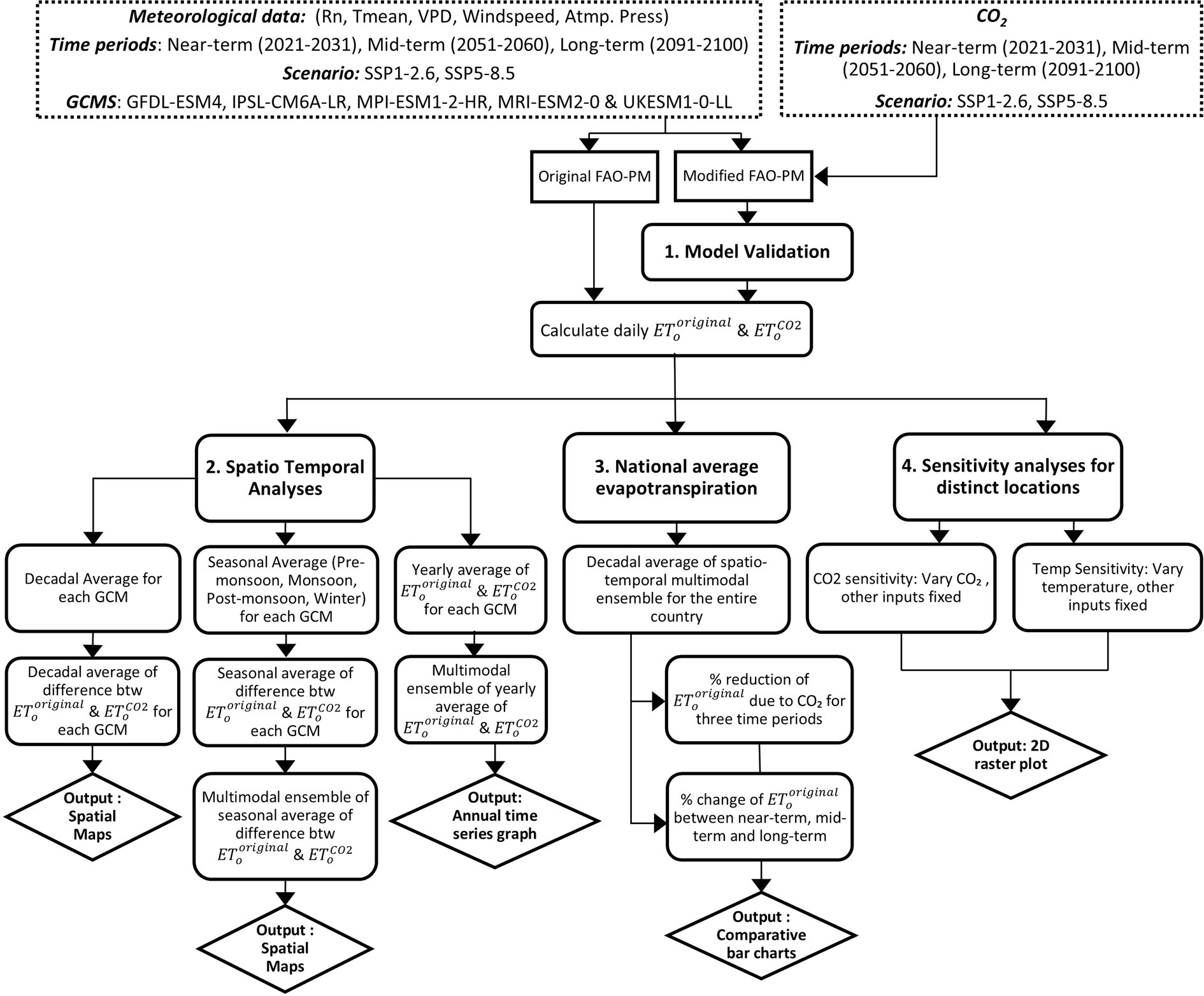
Figure 1. Flow chart summarizing the overall methodology used to assess the impact of rising atmospheric CO₂ on reference evapotranspiration under Indian conditions.

2.1 Scope and study area

The aim of this paper is to demonstrate the extent of disparity between reference evapotranspiration (ET_o) estimated with and without incorporating the influence of CO₂ on contiguous India during three timeframes: the near-term (2021–2030), mid-term (2051–2060) and the long-term (2091–2100) periods. To achieve this, data from five Global Climate Models (GCMs) (see Supplementary Table S1) were obtained from the Inter-Sectoral Impact Model Intercomparison Project (ISIMIP) (Warszawski et al., 2014; Hempel et al., 2013). These five models were chosen because their GCM projections were bias-corrected for the systematic deviation from observations and made freely accessible through the ISIMIP portal of the Potsdam Institute of Climate Impact Research.¹ Furthermore, ISIMIP data effectively capture the uncertainties in global temperature change projections (Ito et al., 2020), which is essential since temperature is an important variable in estimating ET_o.

We focus on two contrasting climate change scenarios: SSP5-8.5 and SSP1-2.6 (see Supplementary Figure S1), which correspond to projected global CO₂ concentrations of approximately 1,130 ppm and 474 ppm, respectively (Büchner and Reyer, 2022). These scenarios are associated with a projected mean temperature rise in India of 4.0-to-4.4 °C under SSP5-8.5 and 1.2-to-1.8 °C under SSP1-2.6 by 2100. We selected SSP5-8.5 because it is commonly used in climate change impact assessment under the worst-case, high-emissions scenario (Jaiswal et al., 2017; Pielke, 2021; Climatedata.ca, 2024), which closely followed observed CO₂ emission trends until recent years (Fuss et al., 2014). In contrast, SSP1-2.6 represents a low-emissions, sustainable development pathway, serving as a benchmark for the most optimistic future with aggressive mitigation.

2.2 Estimation of reference evapotranspiration

We employed two approaches to estimate ET_o, one without considering the effect of atmospheric CO₂ concentration (Equation 1) and the second after incorporating atmospheric CO₂ concentration (Equation 6). The first approach is based on the FAO-PM equation (Allen et al., 1998), which combines the aerodynamic component with the energy component and is idealized for a hypothetical reference crop (Allen et al., 1998). The second approach modifies FAO-PM equation by considering stomatal conductance as a function of atmospheric CO₂ (Equation 5) (Li et al., 2019) instead of a fixed value of surface resistance of 70 s m⁻¹ as used in the original FAO-PM equation (Equation 1) (Allen et al., 1998).

2.3 Derivation of the modified FAO-PM equation

According to the original FAO-PM equation (Allen et al., 1998),

$\begin{array}{ll}{\mathrm{ET}}_{\mathrm{o}}^{\text{original}}=\frac{0.408\Delta ({\mathrm{R}}_{\mathrm{n}}-\mathrm{G})+\gamma \frac{900}{\mathrm{T}+273}{\mathrm{u}}_2({\mathrm{e}}_{\mathrm{s}}-{\mathrm{e}}_{\mathrm{a}})}{\Delta +\gamma (1+0.34{\mathrm{u}}_2)}& (1)\end{array}$

where, ${\mathrm{ET}}_{\mathrm{o}}^{\text{original}}$ is the reference evapotranspiration (mm day⁻¹), R_n is the net radiation (MJ m⁻² day⁻¹) at the canopy surface, G is the soil heat flux density (MJ m⁻² day⁻¹) (G is assumed negligible and hence equals zero), γ is the psychrometric constant (kPa °C⁻¹), T is mean daily air temperature (°C) at 2 m height, u₂ is the wind speed at 2 m height (m s⁻¹), e_s is the saturation vapor pressure (kPa), e_a is the actual vapor pressure (kPa), e_s - e_a is vapor pressure deficit (kPa), and Δ is the slope of the saturated vapor pressure curve (kPa °C⁻¹).

During the formulation of Equation 1, the term $(1+\frac{{\mathrm{r}}_{\mathrm{s}}}{{\mathrm{r}}_{\mathrm{a}}})$ from the Penman-Monteith (PM) model (Monteith, 1965) is substituted with r_s = 70 s m⁻¹ and ${\mathrm{r}}_{\mathrm{a}}=\frac{208}{{\mathrm{u}}_2}$ , to obtain (1 + 0.34u₂). As a first step to incorporating CO₂ in FAO-PM equation, we modify Equation 1 in the following way (Allen et al., 1998; Li et al., 2019; Jarvis et al., 1997):

${\mathrm{r}}_{\mathrm{s}}=\frac{1}{{\mathrm{g}}_{\mathrm{c}}}$

${\mathrm{g}}_{\mathrm{c}}={\mathrm{g}}_{\mathrm{s}}{\mathrm{LAI}}_{\text{active}}$

${\mathrm{LAI}}_{\text{active}}=0.5\mathrm{LAI}$

$\mathrm{LAI}=24\mathrm{h}$

$\mathrm{h}=0.12$

$\text{Hence},{\mathrm{g}}_{\mathrm{c}}=1.44{\mathrm{g}}_{\mathrm{s}}$

$\begin{array}{ll}{\mathrm{r}}_{\mathrm{s}}=\frac{0.694}{{\mathrm{g}}_{\mathrm{s}}}& (2)\end{array}$

$\begin{array}{ll}{\mathrm{r}}_{\mathrm{a}}=\frac{208}{{\mathrm{u}}_2}& (3)\end{array}$

where, r_s is the bulk surface resistance (s m⁻¹), r_a is the aerodynamic resistance (s m⁻¹), g_c is the canopy conductance (m s⁻¹), g_s is the leaf stomatal conductance (m s⁻¹), LAI_active is effective leaf area index (m² m⁻²), h is the hypothetical crop height (equals 0.12 assumed in Equation 1 in m).

Substituting Equations 2, 3 in Equation 1, we get the modified FAO-PM model (Equation 4)

$\begin{array}{ll}{\mathrm{ET}}_{\mathrm{o}}^{\mathrm{CO}2}=\frac{0.408\Delta ({\mathrm{R}}_{\mathrm{n}}-\mathrm{G})+\gamma \frac{900}{\mathrm{T}+273}{\mathrm{u}}_2({\mathrm{e}}_{\mathrm{s}}-{\mathrm{e}}_{\mathrm{a}})}{\Delta +\gamma (1+\frac{0.0033{\mathrm{u}}_2}{{\mathrm{g}}_{\mathrm{s}}})}& (4)\end{array}$

In the above equation, stomatal conductance g_s (m s⁻¹) appears on the right-hand side of Equation 4. Li et al. (2019) developed a modified hyperbolic model that express g_s as a function of atmospheric CO₂ as shown in Equation 5.

$\begin{array}{ll}{\mathrm{g}}_{\mathrm{s}}=\frac{0.0061}{1+0.663(\frac{{\mathrm{CO}}_2}{330}-1)}& (5)\end{array}$

We replaced g_s (m s⁻¹) from Equation 5 to Equation 4 to obtain CO₂ dependent value of reference evapotranspiration ( ${\mathrm{ET}}_{\mathrm{o}}^{\mathrm{CO}2}$ ) (in mm day⁻¹). Our modified version of the FAO-PM equation, presented in Equation 6, provides a simplified representation of ${\mathrm{ET}}_{\mathrm{o}}^{\mathrm{CO}2}$ as a function of atmospheric CO₂, and all the other meteorological inputs used in the original FAO-PM equations (Allen et al., 1998).

$\begin{array}{ll}{\mathrm{ET}}_{\mathrm{o}}^{\mathrm{CO}2}=\frac{0.408\Delta ({\mathrm{R}}_{\mathrm{n}}-\mathrm{G})+\gamma \frac{900}{\mathrm{T}+273}{\mathrm{u}}_2({\mathrm{e}}_{\mathrm{s}}-{\mathrm{e}}_{\mathrm{a}})}{\Delta +\gamma (1+0.541{\mathrm{u}}_2(1+0.663(\frac{{\mathrm{CO}}_2}{330}-1)\left)\right)}& (6)\end{array}$

2.4 Data for validating the modified FAO-PM equation

To validate our proposed modified FAO-PM equation, we used measured data from six independent sites included in the AmeriFlux network (Novick et al., 2018), which is a part of the global FLUXNET (Pastorello et al., 2020) network of eddy covariance towers.² The six sites were selected based on details provided about vegetation and/or crop cover, availability of crop coefficients, and availability of the planting and harvest dates (see Supplementary Table S2; Nass, 2010). They comprise of four agricultural and natural vegetation types including alfalfa cultivation (Twitchell and Bouldin Islands), managed pastures (Medford hay pasture), irrigated croplands (continuous maize at Mead) and native prairie ecosystems (Rosemount Prairie and Konza prairie; see Supplementary Table S2). All of the sites also span across different types of climates. Twitchell alfalfa and Bouldin islands come under the Csa Koppen climate classification (Mediterranean) with mild winters and dry hot summers. Medford hay pasture and Konza Prairie exhibits Cfa climate (Humid subtropical) with mild winters, hot summers and year-round rainfall. Rosemount prairie and Mead’s maize site experience a Dfa climate (Humid Continental) with severe winters, hot summers, and no dry season. The downloaded data from the AmeriFlux site consisted of the following variables; air temperature, vapor pressure deficit, net radiation, wind speed, atmospheric pressure, atmospheric CO₂ and latent heat flux. Additionally, weather data from two representative stations located in the southern Indian state of Kerala were used to compare model performance: one at Trivandrum (8.544°N, 76.913°E) and the other at Palakkad (10.807°N, 76.7258°E). These datasets were used to compare the performance between the modified FAO-PM equation and two other methods: the original FAO-PM equation (Allen et al., 1998) and the widely used Priestley-Taylor equation (Priestley and Taylor, 1972).

2.5 Validation approach

We converted the daily observed latent heat flux data into actual evapotranspiration by dividing latent heat flux with latent heat of vaporization [λ = 2.45 MJ kg⁻¹ (Allen et al., 1998)] (see Supplementary Equation S1). The actual evapotranspiration was then divided by crop coefficients (see Supplementary Table S2) corresponding to vegetation type (see Supplementary Equation S2) to estimate reference evapotranspiration ( ${\mathrm{ET}}_{\mathrm{o}}^{\mathrm{obs}}$ ). We used ${\mathrm{ET}}_{\mathrm{o}}^{\mathrm{obs}}$ to validate our predictions of ${\mathrm{ET}}_{\mathrm{o}}^{\mathrm{CO}2}$made using modified FAO-PM equation (Equation 6) for the six sites.

To compare our model estimations against commonly used approaches for selected sites in India, we used the weather data from specific stations in the South Indian state of Kerala (see Supplementary Table S3) to estimate reference evapotranspiration using both the original and modified FAO-PM models. Additionally, the ${\mathrm{ET}}_{\mathrm{o}}^{\mathrm{CO}2}$ values were further compared with the estimated values by the Priestley-Taylor equation, based on the same weather station data.

The statistics used for the validation and comparison were Root Mean Square Error (RMSE in mm day⁻¹), coefficient of determination (R²), and the correlation coefficient (r) (see Supplementary Equations S3–S5).

2.6 Climate data for regional simulations

The climate data to estimate ET_o across India was obtained from the Inter-Sectoral Impact Model Intercomparison Project (ISIMIP), ISIMIP3b protocol (Hempel et al., 2013; Warszawski et al., 2014). The ISIMIP project provides bias-corrected gridded global climate projection data from 1800 to 2100 at daily (and coarser) time steps with a spatial resolution of 0.5° × 0.5°. We used projected climate data for contiguous India for the period from 2021–2030 (near-term), 2051–2060 (mid-term), and 2091–2100 (long-term) corresponding to the five GCMs, namely GFDL-ESM4, IPSL-CM6A-LR, MPI-ESM1-2-HR, MRI-ESM2-0, and UKESM1-0-LL under SSP1-2.6 and SSP5–8.5 scenarios (Lange and Büchner, 2021; see Supplementary Table S1). We downloaded six variables, namely near surface relative humidity, surface air pressure, surface downwelling shortwave radiation, near surface wind speed, daily maximum near surface temperature, and minimum near surface air temperature (Lange and Büchner, 2021). Additionally, ISIMIP3b atmospheric composition input data for annual mean CO₂ concentrations under SSP5-8.5 and SSP1-2.6 (Büchner and Reyer, 2022) was also downloaded (see Supplementary Figure S1) to calculate ${\mathrm{ET}}_{\mathrm{o}}^{\mathrm{CO}2}$ using modified FAO-PM equation (Equation 6). The soil heat flux density (G) was assumed to be negligible in our calculations (Allen et al., 1998; Varghese and Mitra, 2024).

2.7 Estimations for spatio-temporal analyses

We estimated the daily ${\mathrm{ET}}_{\mathrm{o}}^{\text{original}}$ (Equation 1) and ${\mathrm{ET}}_{\mathrm{o}}^{\mathrm{CO}2}$ (Equation 6) for each year from 2021–2030 (near-term), 2051–2060 (mid-term) and 2091–2100 (long-term) across contiguous India using data from each of the five GCMs for both the scenarios (SSP1-2.6 and SSP5-8.5). From this point forward, any reference to India refers to contiguous India.

(a) Decadal averages of ${\mathrm{ET}}_{\mathrm{o}}^{\text{original}}$and ${\mathrm{ET}}_{\mathrm{o}}^{\mathrm{CO}2}$ were computed to conduct spatial analyses across India. Intra-decadal trends in the yearly averaged values of ${\mathrm{ET}}_{\mathrm{o}}^{\text{original}}$ and ${\mathrm{ET}}_{\mathrm{o}}^{\mathrm{CO}2}$ spatially averaged across India were also analyzed.

(b) We also calculated the daily difference between ${\mathrm{ET}}_{\mathrm{o}}^{\text{original}}$ and ${\mathrm{ET}}_{\mathrm{o}}^{\mathrm{CO}2}$ for each GCM, time period, and scenario. These differences were averaged over each decade and mapped to analyze spatial patterns across India.

(c) To assess seasonal variability, daily estimates of ${\mathrm{ET}}_{\mathrm{o}}^{\text{original}}$ and ${\mathrm{ET}}_{\mathrm{o}}^{\mathrm{CO}2}$were grouped into four seasons following Jhajharia et al. (2009): winter (Jan–Feb), pre-monsoon (Mar–May), monsoon (Jun–Sep), and post-monsoon (Oct–Dec).

Thereafter, seasonal averages were computed for each GCM, time period, and scenario. The differences between seasonal ${\mathrm{ET}}_{\mathrm{o}}^{\text{original}}$ and ${\mathrm{ET}}_{\mathrm{o}}^{\mathrm{CO}2}$ were then calculated for each GCM and these differences were averaged across all five GCMs to obtain an overall seasonal difference.

Maps were classified using manually determined class breaks after identifying the minimum and maximum values projected by all GCMs for each step (ESRI, 2024).

2.8 Estimating the impact of CO₂ on the national average evapotranspiration

To quantify relative impact of incorporating CO₂ on national average evapotranspiration we have calculated ${\mathrm{ET}}_{\mathrm{o},\text{near}-\text{term}}^{\text{original}}$ , ${\mathrm{ET}}_{\mathrm{o},\mathrm{mid}-\text{term}}^{\text{original}}$ and ${\mathrm{ET}}_{\mathrm{o},\text{long}-\text{term}}^{\text{original}}$ , which represent spatio-temporal averages (for entire country over a period of 10 years) of ET_o estimated using the original FAO-PM (Equation 1) for near-term period (2021–2030), mid-term (2051–2060) and long-term periods (2091–2100), respectively. Similarly, we calculated ${\mathrm{ET}}_{\mathrm{o},\text{near}-\text{term}}^{\mathrm{CO}2}$ , ${\mathrm{ET}}_{\mathrm{o},\mathrm{mid}-\text{term}}^{\mathrm{CO}2}$ and ${\mathrm{ET}}_{\mathrm{o},\text{long}-\text{term}}^{\mathrm{CO}2}$ , which represent the spatio-temporal averages of ${\mathrm{ET}}_{\mathrm{o}}^{\mathrm{CO}2}$ estimated using the modified FAO-PM (Equation 6). We calculated percentage change in ${\mathrm{ET}}_{\mathrm{o}}^{\text{original}}$ , as we move from near-term to mid-term $(100\times ({\mathrm{ET}}_{\mathrm{o},\text{near}-\text{term}}^{\text{original}}$ – ${\mathrm{ET}}_{\mathrm{o},\mathrm{mid}-\text{term}}^{\text{original}})÷{\mathrm{ET}}_{\mathrm{o},\text{near}-\text{term}}^{\text{original}})$ , and long-term $(100\times ({\mathrm{ET}}_{\mathrm{o},\text{near}-\text{term}}^{\text{original}}$ – ${\mathrm{ET}}_{\mathrm{o},\text{long}-\text{term}}^{\text{original}})÷{\mathrm{ET}}_{\mathrm{o},\text{near}-\text{term}}^{\text{original}})$ with the assumption that original FAO-PM equation would be continued to be used. Similarly, we also calculated percentage changes in the estimated ET_o as a result of incorporating CO₂ for near-term $(100\times ({\mathrm{ET}}_{\mathrm{o},\text{near}-\text{term}}^{\text{original}}$ – ${\mathrm{ET}}_{\mathrm{o},\text{near}-\text{term}}^{\mathrm{CO}2})÷{\mathrm{ET}}_{\mathrm{o},\text{near}-\text{term}}^{\text{original}}$ ), mid-term $(100\times ({\mathrm{ET}}_{\mathrm{o},\mathrm{mid}-\text{term}}^{\text{original}}$ – ${\mathrm{ET}}_{\mathrm{o},\mathrm{mid}-\text{term}}^{\mathrm{CO}2})÷{\mathrm{ET}}_{\mathrm{o},\mathrm{mid}-\text{term}}^{\text{original}}$ ), and long-term periods $(100\times ({\mathrm{ET}}_{\mathrm{o},\text{long}-\text{term}}^{\text{original}}$ – ${\mathrm{ET}}_{\mathrm{o},\text{long}-\text{term}}^{\mathrm{CO}2})÷{\mathrm{ET}}_{\mathrm{o},\text{long}-\text{term}}^{\text{original}}$ ) using ${\mathrm{ET}}_{\mathrm{o}}^{\text{original}}$ as base value.

2.9 Sensitivity analysis

After the spatio-temporal analyses, we identified two locations in India which exhibit drastically different response of rising CO₂ and temperature on ET_o. These two locations were used to conduct a sensitivity analysis of ${\mathrm{ET}}_{\mathrm{o}}^{\mathrm{CO}2}$ with respect to temperature and atmospheric CO₂. To perform the sensitivity analysis, the CO₂ concentration was varied from 400 to 1,200 ppm while keeping all the remaining input parameters unchanged. Similarly, temperature sensitivity analysis was done by varying temperature from 18 to 34 °C while keeping all the remaining input parameters unchanged. These ranges were determined based on meteorological data for the three decadal periods for these two specific locations. The values of all the other variables during sensitivity analysis were kept constant based on their average values and are given in Supplementary Table S4. All the data produced during this analyses is available publicly as an archive (Surendran et al., 2025).

3 Results

3.1 Model validation and comparison

We developed the modified FAO-PM (Equation 6) which effectively predicted the daily reference evapotranspiration ( ${\mathrm{ET}}_{\mathrm{o}}^{\mathrm{CO}2}$ ) at the six AmeriFlux (Novick et al., 2018) sites (Figure 2) with atmospheric CO₂ concentrations ranging from 370 ppm in 2001 to 418 ppm in 2021 (see Supplementary Table S2). The correlation coefficient (r) indicates moderate to strong linear relationships between the observed $({\mathrm{ET}}_{\mathrm{o}}^{\mathrm{obs}}$ – see Supplementary Equation S2) and estimated ET_o using Equation 6 ( ${\mathrm{ET}}_{\mathrm{o}}^{\mathrm{CO}2}$ ), with the site US-A32 showing the highest correlation (r = 0.72) and the site US-Ne1 showing the lowest correlation (r = 0.606). The slopes of the regression lines through the origin ranged from 0.8 to 1.04, demonstrating close alignment with the 1:1 line across all six sites (Figure 2). RMSE values ranged from 1.152 to 1.566 mm day⁻¹, with the site US-Ro4 exhibiting the lowest RMSE and the site US-Bi1 showing the highest.

Figure 2

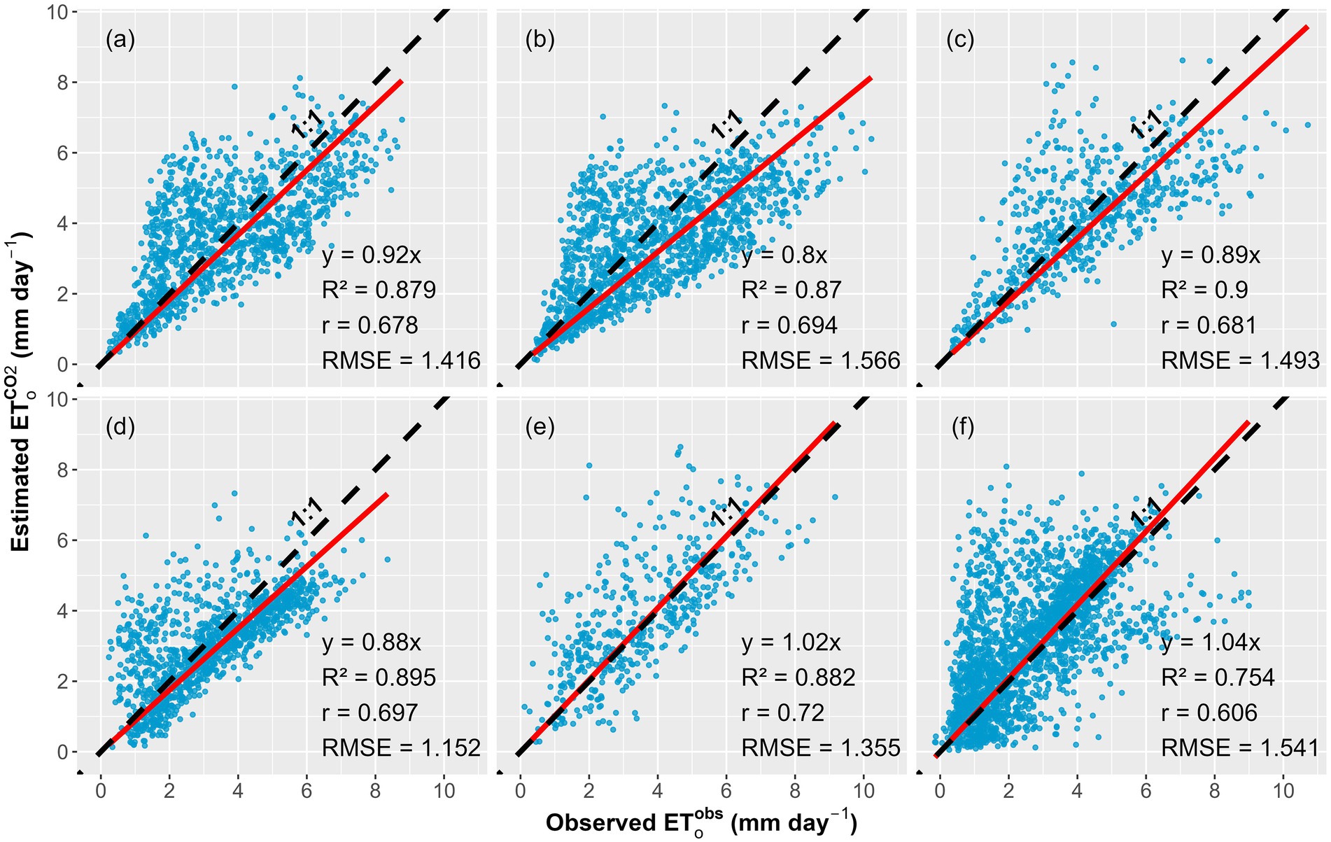
Figure 2. Scatter plots of the comparison between the observed rates of reference evapotranspiration ( ${\mathrm{ET}}_{\mathrm{o}}^{\mathrm{obs}}$in mm day⁻¹) and predicted rates of reference evapotranspiration ( ${\mathrm{ET}}_{\mathrm{o}}^{\mathrm{CO}2}$ in mm day⁻¹) using the FAO-PM equation modified to incorporate the impact of atmospheric CO₂ concentration on surface resistance at the six AmeriFlux sites (a) US-Tw3: Twitchell Alfalfa (2013–2018), (b) US-Bi1: Bouldin Island Alfalfa (2016–2021), (c) US-xKZ: NEON Konza Prairie Biological Station (KONZ) (2017–2021) (d) US-Ro4: Rosemount Prairie (2014–2021), (e) US-A32: ARM-SGP Medford hay pasture (2015–2017) and (f) US-Ne1: Mead - irrigated continuous maize site (2001–2020).

To compare the estimation of the modified FAO PM equation (Equation 6) against commonly used methods for selected Indian sites, we used daily weather data from two stations located in the southern Indian state of Kerala: Trivandrum (8.544°N, 76.913°E) and Palakkad (10.807°N, 76.7258°E). Using this data, reference evapotranspiration was estimated using the original FAO-PM model (ETₒ FAO–PM), the modified CO₂-sensitive FAO-PM model ( ${\mathrm{ET}}_{\mathrm{o}}^{\mathrm{CO}2}$ ), and the Priestley-Taylor model (ET_PT). Figure 3 compares ${\mathrm{ET}}_{\mathrm{o}}^{\mathrm{CO}2}$ with ET_o FAO–PM and ET_PT for both locations. The modified FAO-PM model exhibited a strong agreement with the original FAO-PM model at both sites, with high R² values (0.999 for Trivandrum and 0.988 for Palakkad), strong correlation coefficients (r = 0.996 and 0.992, respectively), and low RMSE values (0.084 and 0.329-mm day⁻¹, respectively). Comparisons with the Priestley-Taylor model showed relatively lower agreement, with higher RMSE values (0.486 and 0.887 mm day⁻¹, respectively) and underprediction tendencies (slopes of 0.82 and 0.76, respectively).

Figure 3

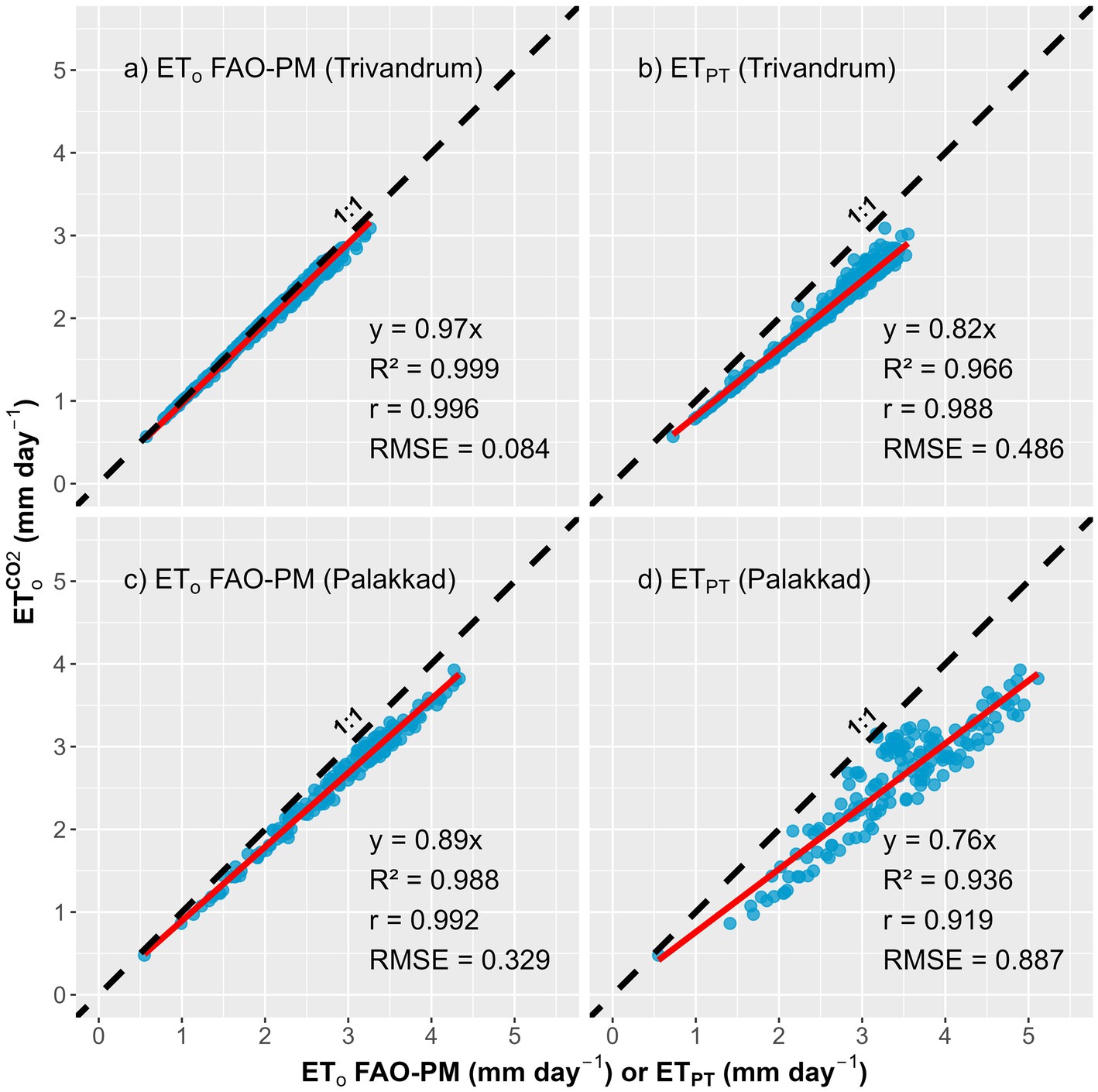
Figure 3. Scatter plots of the comparison between daily reference evapotranspiration estimates from the modified FAO Penman-Monteith model ( ${\mathrm{ET}}_{\mathrm{o}}^{\mathrm{CO}2}$ in mm day⁻¹) with those from the original FAO-PM model (ETₒ FAO–PM) and the Priestley-Taylor equation (ET_PT) using observed weather data at two locations in Kerala, India; Trivandrum (8.544°E, 76.913°N) and Palakkad (10.807°E, 76.7258°N). Panels (a) and (c) compare ${\mathrm{ET}}_{\mathrm{o}}^{\mathrm{CO}2}$ with ETₒ FAO–PM, while panels (b) and (d) compare ${\mathrm{ET}}_{\mathrm{o}}^{\mathrm{CO}2}$with ET_PT.

3.2 Spatio-temporal variations in $E{T}_o^{\mathit{\text{original}}}$ and $E{T}_o^{\mathit{CO}2}$

Analyses of ${\mathrm{ET}}_{\mathrm{o}}^{\text{original}}$ and ${\mathrm{ET}}_{\mathrm{o}}^{\mathrm{CO}2}$ under SSP1-2.6 and SSP5-8.5 scenario utilizing five GCMs (see Supplementary Table S1; Supplementary Figure S1) during near-term (2021–2030), mid-term (2051–2060) and long-term (2091–2100) periods, and all spatial locations in India, showed that the former exceeded the latter consistently in all cases (Figure 4) due to the impact of rising atmospheric CO₂ concentration that was not included in the original FAO-PM model (Equation 1). In general, both ${\mathrm{ET}}_{\mathrm{o}}^{\text{original}}$and ${\mathrm{ET}}_{\mathrm{o}}^{\mathrm{CO}2}$ , are decreasing as we move from west to east for all cases (Figure 4). The highest values of ${\mathrm{ET}}_{\mathrm{o}}^{\text{original}}$and ${\mathrm{ET}}_{\mathrm{o}}^{\mathrm{CO}2}$ (Figure 4) and the difference between ${\mathrm{ET}}_{\mathrm{o}}^{\text{original}}$and ${\mathrm{ET}}_{\mathrm{o}}^{\mathrm{CO}2}$ (Figure 5) were observed covering parts of desert regions in Rajasthan by all the five GCMs for all the time periods and scenarios.

Figure 4

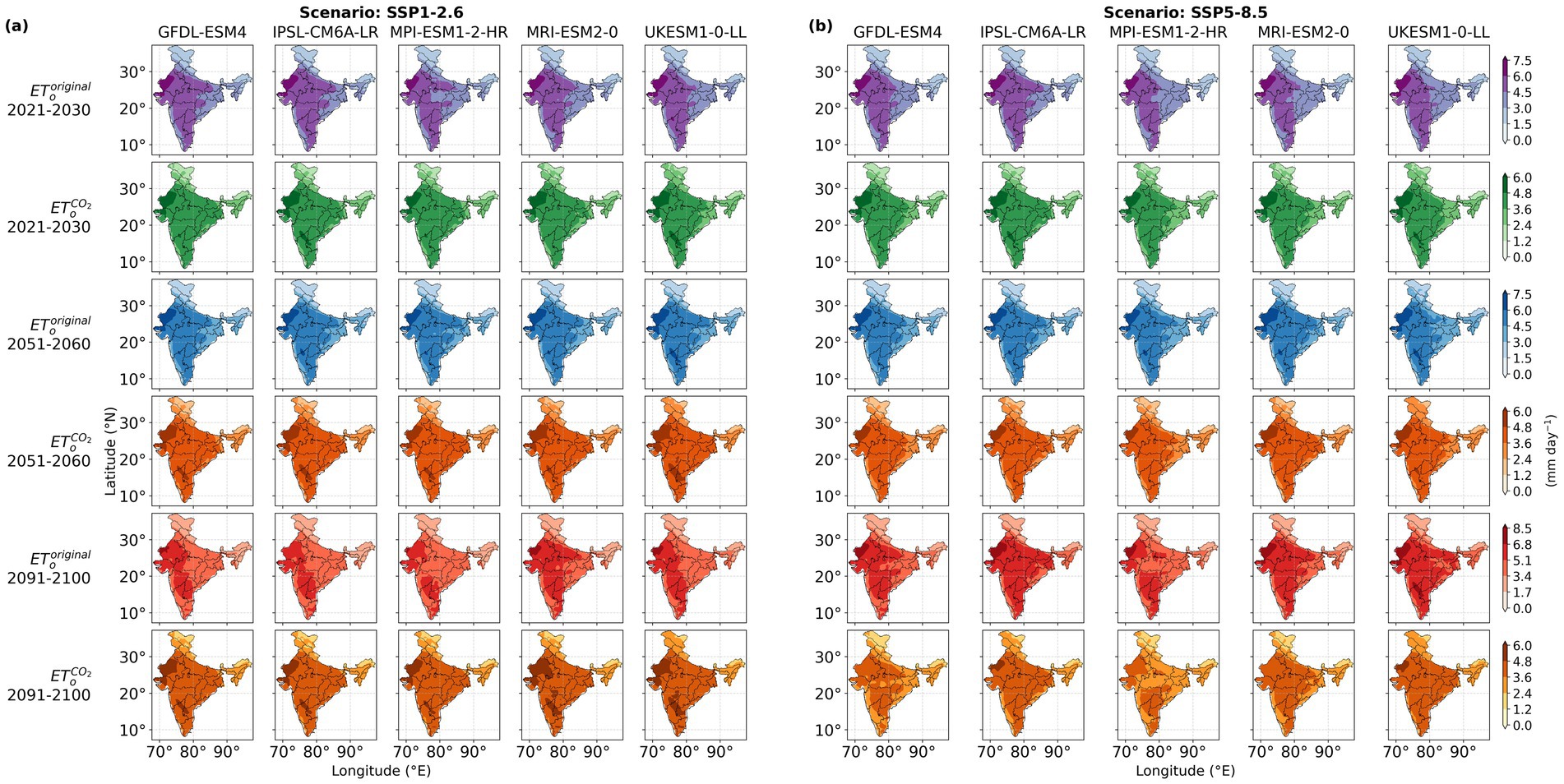
Figure 4. Decadal average of ${\mathrm{ET}}_{\mathrm{o}}^{\text{original}}$and ${\mathrm{ET}}_{\mathrm{o}}^{\mathrm{CO}2}$in mm day⁻¹ for near-term, mid-term and long-term periods across India for the five GCMs under (a) SSP1-2.6 and (b) SSP5-8.5.

Figure 5

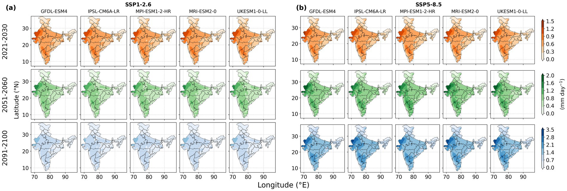
Figure 5. The decadal average of difference between ${\mathrm{ET}}_{\mathrm{o}}^{\text{original}}$and ${\mathrm{ET}}_{\mathrm{o}}^{\mathrm{CO}2}$projected by each of the five GCM’s for near-term, mid-term and long-term across India under (a) SSP1-2.6 and (b) SSP5-8.5.

While the differences between ${\mathrm{ET}}_{\mathrm{o}}^{\text{original}}$ and ${\mathrm{ET}}_{\mathrm{o}}^{\mathrm{CO}2}$ were similar for both SSP1-2.6 and SSP5-8.5 in the near term, they became significantly larger under SSP5-8.5 during the mid-term and long-term time periods, indicating divergent temporal trajectories across the two scenarios (Figure 5). The regions predicted to have lowest values of ${\mathrm{ET}}_{\mathrm{o}}^{\text{original}}$ and ${\mathrm{ET}}_{\mathrm{o}}^{\mathrm{CO}2}$ (Figure 4) and their difference (Figure 5) included high-altitude deserts of Ladakh and northeastern states.

The spatially averaged values of ${\mathrm{ET}}_{\mathrm{o}}^{\text{original}}$ and ${\mathrm{ET}}_{\mathrm{o}}^{\mathrm{CO}2}$ across India (Figure 6) indicated a small variation in the time-series of estimated values within a period of 10-years corresponding to the near-term, mid-term and long-term time periods for all the GCMs and under both SSP1-2.6 and SSP5-8.5 scenarios. The predicted values of ${\mathrm{ET}}_{\mathrm{o}}^{\text{original}}$ was consistently higher than ${\mathrm{ET}}_{\mathrm{o}}^{\mathrm{CO}2}$ for all the scenarios and time periods. The differences between the two were largest for the long-term (2091–2100) period under SSP5-8.5 when CO₂ concentrations are projected to reach 1,130 ppm (see Supplementary Figure S1).

Figure 6

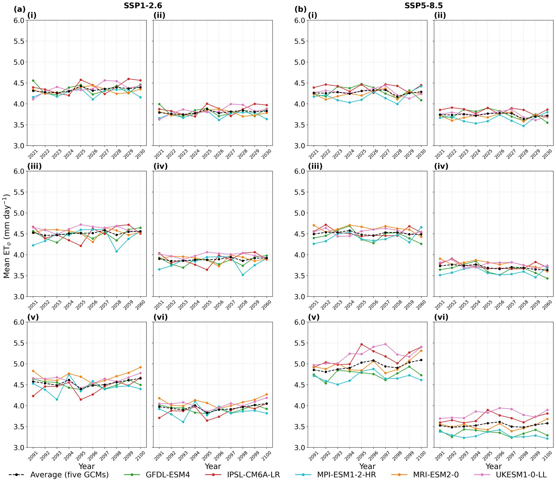
Figure 6. Annual time series of (i) ${\mathrm{ET}}_{\mathrm{o}}^{\text{original}}$ for near-term (2021–2030) (ii) ${\mathrm{ET}}_{\mathrm{o}}^{\mathrm{CO}2}$for near-term (iii) ${\mathrm{ET}}_{\mathrm{o}}^{\text{original}}$ for mid-term (2051–2060) (iv) ${\mathrm{ET}}_{\mathrm{o}}^{\mathrm{CO}2}$for mid-term (v) ${\mathrm{ET}}_{\mathrm{o}}^{\text{original}}$ for long-term (2091–2100) and (vi) ${\mathrm{ET}}_{\mathrm{o}}^{\mathrm{CO}2}$for long-term obtained using five GCMs and their overall average under (a) SSP1-2.6 and (b) SSP5-8.5.

3.3 Seasonal variations in the ET_o difference

Spatial variations in the magnitude of the differences between ${\mathrm{ET}}_{\mathrm{o}}^{\text{original}}$ and ${\mathrm{ET}}_{\mathrm{o}}^{\mathrm{CO}2}$for the four seasons are seen in all three time periods under both the scenarios (Figure 7). The differences between ${\mathrm{ET}}_{\mathrm{o}}^{\text{original}}$ and ${\mathrm{ET}}_{\mathrm{o}}^{\mathrm{CO}2}$was the largest during the pre-monsoon season, in most parts of India except the far-northern and north-eastern states. The lowest differences were observed during the post-monsoon and winter season (Figure 7). Spatially, the magnitude of these differences for the winter and post-monsoon seasons were the least in the northern and north-eastern regions and highest in major parts of Rajasthan, Gujarat, Maharashtra and southern India for all time periods and scenarios. The differences were higher for the long-term period than for the near-term period and mid-term period only under scenario SSP5-8.5 for all the locations and seasons. Under the SSP1-2.6 scenario, the differences were smaller and ranged from 0.05 to 2.5 mm day⁻¹ across all seasons and time periods.

Figure 7

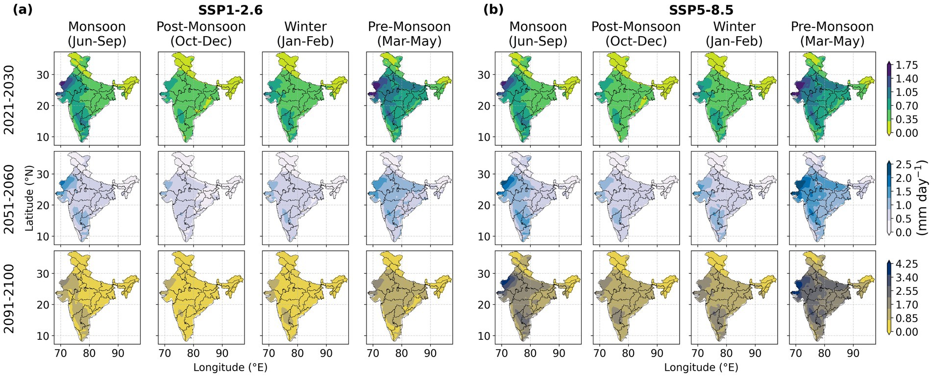
Figure 7. Average of difference between ${\mathrm{ET}}_{\mathrm{o}}^{\text{original}}$ and ${\mathrm{ET}}_{\mathrm{o}}^{\mathrm{CO}2}$obtained using five GCMs, corresponding to four seasons for near-term, mid-term and long-term periods under (a) SSP1-2.6 and (b) SSP5-8.5.

The absolute spatio-temporal average values of the seasonal (monsoon, post-monsoon, winter, and pre-monsoon) variations of ${\mathrm{ET}}_{\mathrm{o}}^{\text{original}}$ and ${\mathrm{ET}}_{\mathrm{o}}^{\mathrm{CO}2}$for the near-term, mid-term and long-term periods under SSP1-2.6 and SSP5-8.5 are shown in Table S5 and S6, respectively (see Supplementary material) for the five GCMs. The seasonal patterns are nearly consistent among GCMs with higher values of ${\mathrm{ET}}_{\mathrm{o}}^{\text{original}}$ and ${\mathrm{ET}}_{\mathrm{o}}^{\mathrm{CO}2}$observed during pre-monsoon and lower values observed during the post-monsoon and winter season for all the three simulation periods and scenarios. All seasons show a decrease in the predicted ET_o when incorporating the effect of CO₂ for SSP5-8.5 (see Supplementary Tables S5, S6).

3.4 Sensitivity analyses of $E{T}_o^{\mathit{CO}2}$

The sensitivity analysis of ${\mathrm{ET}}_{\mathrm{o}}^{\mathrm{CO}2}$ with respect to temperature and CO₂ concentration (Figure 8) revealed distinct trends at both the locations selected. Location 1 (26.75°N, 70.25°E), situated in the arid desert region of Rajasthan with a hot desert climate, exhibited ${\mathrm{ET}}_{\mathrm{o}}^{\mathrm{CO}2}$ values ranging from 3.22 to 9.65 mm day⁻¹ as CO₂ concentration increased from 400 to 1,200 ppm and temperature was varied from 26 to 33 °C. This location showed the greatest difference in ET_o​ estimated using original and modified FAO-PM equations. Location 2 (23.75°N, 93.25°E), situated in Arunachal Pradesh with a tropical rainforest climate, showed ${\mathrm{ET}}_{\mathrm{o}}^{\mathrm{CO}2}$ values ranging from 0.6 to 1.35 mm day⁻¹ for the same CO₂ range and temperature variation from 18 to 24 °C. This location exhibited the lowest difference in ET_o estimated using original and modified FAO-PM equations.

Figure 8

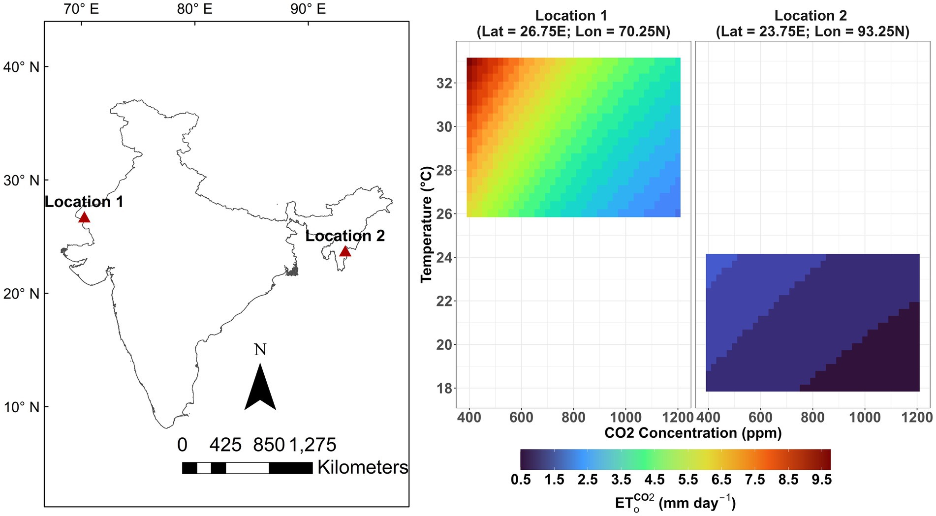
Figure 8. Interaction of CO₂, temperature and ${\mathrm{ET}}_{\mathrm{o}}^{\mathrm{CO}2}$ at location 1 (26.75°N, 70.25°E) and location 2 (23.75°N, 93.25°E). These locations are characterized by highest (location 1) and lowest (location 2) differences of ${\mathrm{ET}}_{\mathrm{o}}^{\text{original}}$ and ${\mathrm{ET}}_{\mathrm{o}}^{\mathrm{CO}2}$ .

3.5 Impact of CO₂ on the national average evapotranspiration

Spatio-temporal averages across India (Figure 9) shows that incorporating CO₂ concentrations in calculating ET_o results in a reduction of 12.4, 13.9, and 13.0% for near-term, mid-term, and long-term time periods respectively under SSP1-2.6. Under SSP5-8.5, the percentage difference (12.6%) was more-or-less similar to the ones observed under SSP1-2.6 for the near-term period but were much larger for the mid-term and long-term periods (18.0 and 29%, respectively).

Figure 9

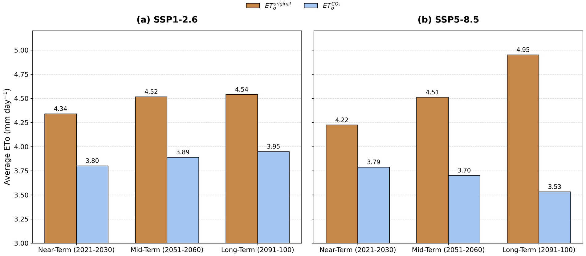
Figure 9. ET_o averaged over the entire country for near-term, mid-term and long-term periods under (a) SSP1-2.6 and (b) SSP5-8.5 using climate data from five GCMs (GFDL-ESM4, IPSL-CM6A-LR, MPI-ESM1-2-HR, MRI-ESM2-0, and UKESM1-0-LL).

If one continues to use original FAO-PM equation (Equation 1), which does not consider the effect of rising CO_2, then the increase in the ET_o is expected to be 4.0 and 4.6% as we move from near-term (2021–2030) to mid-term (2051–2060), and near-term to long-term (2091–2100) periods, respectively, under scenario SSP1-2.6. These numbers change to 6.0 and 16.0%, respectively under the scenario SSP5-8.5.

4 Discussion

4.1 Reliability of modified FAO-PM equation spans a wide variety of vegetation types and climatic conditions

Our model performed satisfactorily against the AmeriFlux network data (Novick et al., 2018), with R² values ranging from 0.75 to 0.90 (Figure 2). These values are comparable to those reported by Li et al. (2019), who found R² values of 0.76 to 0.83 while validating ${\mathrm{ET}}_{\mathrm{o}}^{\mathrm{CO}2}$ against water balance-based estimates for maize under controlled conditions. In contrast, our validation included six sites with diverse vegetation types and management practices (see Supplementary Table S2), where site selection was guided by the availability of crop coefficient (Basketfield, 1985; Allen et al., 1998; Nass, 2010; Pereira et al., 2023), which is essential for converting actual evapotranspiration (ET_actual) (see Supplementary Equation S1) from eddy covariance towers to ${\mathrm{ET}}_{\mathrm{o}}^{\mathrm{obs}}$ using crop coefficients (see Supplementary Equations S1, S2). The greater scatter observed in our validation plot (Figure 2) can be attributed to uncertainties in crop coefficients (Peng et al., 2019), as well as site-specific factors such as spatial heterogeneity, variations in planting and harvest dates, irrigation practices, environmental stresses, and other management practices.

The comparison of the modified FAO-PM model using daily weather data from two locations in Kerala, Palakkad and Trivandrum, showed strong agreement with the original FAO-PM formulation, yielding high R² values (0.98 to 0.99) (Figure 3). These sites represent typical humid tropical environments characterized by high moisture availability and seasonal variability, making them suitable test references for model evaluation in such climates. Palakkad includes agriculturally important areas, further supporting the relevance of these results. The high agreement with the original FAO-PM method suggests that the modified model preserves the core structure and reliability of the standard formulation while integrating the physiological response of vegetation to elevated CO₂. Previous studies, such as Nandagiri and Kovoor (2006) have shown that radiation-based models like Priestley-Taylor (PT) perform reasonably well in humid regions. Supporting this, our comparison of ${\mathrm{ET}}_{\mathrm{o}}^{\mathrm{CO}2}$with ET_PT at both Kerala locations showed strong statistical relationships (R² = 0.936-to-0.966; r = 0.919-to-0.988), indicating that PT captures the temporal patterns of evapotranspiration well. However, the slopes of the lines (0.76 and 0.82) and relatively higher RMSE values (0.486 to 0.887 mm day⁻¹) point to a consistent underestimation by the PT method compared to the modified FAO-PM model (Figure 3). This underprediction highlights the advantage of including physiological and aerodynamic controls, as well as CO₂ sensitivity, which are absent in simpler radiation-based models.

Together, these results show that the modified FAO-PM model not only performs reliably under controlled or semi-controlled conditions but also maintains robustness across complex, real-world scenarios. This consistency across different climates, vegetation types, and data sources supports the model’s potential for large-scale applications in climate impact studies and agricultural water management.

4.2 Impacts of incorporating changing CO₂ concentrations across the three decadal periods

The CO₂ range in the validation data for the modified FAO-PM equation (Equation 6) was relatively narrow (370–418 ppm) (see Supplementary Table S2), reflecting past natural environmental conditions. However, this modified FAO-PM equation (Equation 6) has been previously validated under controlled conditions with CO₂ levels up to 900 ppm (Li et al., 2019). This higher level is comparable to the atmospheric CO₂ concentrations projected by the SSP5-8.5 scenario in the long-term period (2091–2100) (see Supplementary Figure S1), considered in our study to evaluate the spatial variation of the impact of CO₂ on ET_o across India (Figures 4b, 5b).

We predicted a consistent trend of ${\mathrm{ET}}_{\mathrm{o}}^{\mathrm{CO}2}$being less than ${\mathrm{ET}}_{\mathrm{o}}^{\text{original}}$ (Figures 4, 5) due to the CO₂ impacts on stomatal closure, which is similar to reported trends in previous studies (Li et al., 2019; Yang et al., 2019; Varghese and Mitra, 2024). In our knowledge, the absolute values of ${\mathrm{ET}}_{\mathrm{o}}^{\mathrm{CO}2}$ and ${\mathrm{ET}}_{\mathrm{o}}^{\text{original}}$ covering whole India have not been reported previously. The predicted ${\mathrm{ET}}_{\mathrm{o}}^{\text{original}}$ for the near-term period ranged from 1.94-to-7.04 mm day⁻¹ under both SSP1-2.6 and SSP5-8.5 (Figure 4), aligning with recent estimates done for smaller regions within India (Jhajharia et al., 2009; Nag et al., 2014; Pandey et al., 2016; Das et al., 2023). The increase in ${\mathrm{ET}}_{\mathrm{o}}^{\text{original}}$ from the near-term to long-term (Figure 4b) can be attributed to rising temperatures under SSP5-8.5, as studies have shown a positive correlation between temperature and ET_o (Wang et al., 2022; Zhou et al., 2022) with temperature contributing up to 45% of ET_o variation (Varghese and Mitra, 2024). However, this increase in ET_o is moderated ( ${\mathrm{ET}}_{\mathrm{o}}^{\mathrm{CO}2}$ < ${\mathrm{ET}}_{\mathrm{o}}^{\text{original}}$ in Figure 4) as a consequence of incorporating the effect of CO₂ in our calculations. Estimations using all five GCMs (Figures 4, 5) are consistent in predicting the ${\mathrm{ET}}_{\mathrm{o}}^{\mathrm{CO}2}$ to be less than the ${\mathrm{ET}}_{\mathrm{o}}^{\text{original}}$ but they differ in the magnitude as well as spatial variations of the differences. The spatial averages (Figure 6) reveal no distinct temporal trends within 10-year intervals for either the near-term or long-term periods across all GCMs. However, transitioning from the near-term to long-term period highlights the dominant influence of CO₂ on ET_o, with reductions in ET_o due to elevated CO₂ levels outweighing increases driven by rising temperatures under SSP5-8.5 (Figure 6b). Consequently, long-term ${\mathrm{ET}}_{\mathrm{o}}^{\mathrm{CO}2}$ is projected to be lower than the current estimates, under the SSP5-8.5 scenario, contrary to several previous studies (Liu et al., 2020; Zhai et al., 2020) that did not account for the impact of CO₂.

The spatial variability of differences between ${\mathrm{ET}}_{\mathrm{o}}^{\mathrm{CO}2}$ and ${\mathrm{ET}}_{\mathrm{o}}^{\text{original}}$ (Figure 5) is influenced by climate inputs beyond CO₂ as shown in the sensitivity analyses of the modified FAO-PM (Equation 6) for two distinct locations (Figure 8). Location 1 (26.75°N, 70.25°E), characterized by the hot desert climate in the northwest, exhibits a pronounced response to rising CO₂, with ${\mathrm{ET}}_{\mathrm{o}}^{\mathrm{CO}2}$ ranging from 3.22-to-9.65 mm day⁻¹, as CO₂ concentration increases from 400 to 1,200 ppm and temperature varies from 26-to-33 °C. In contrast, Location 2 (23.75°N, 93.25°E), characterized by a tropical rainforest climate of the northeast, shows minimal response, with ${\mathrm{ET}}_{\mathrm{o}}^{\mathrm{CO}2}$ values varying from 0.6-to-1.35 mm day⁻¹ for the same CO₂ range and temperature variation from 18-to-33 °C. This non-linear, location-specific interaction between CO₂, temperature, and ET_o may help explain deviations from the typically positive correlation between ET_o and temperature (Wang et al., 2022; Zhou et al., 2022), a phenomenon often referred to as the “evapotranspiration paradox” (Rao and Wani, 2011; Varghese and Mitra, 2024). The “evapotranspiration paradox” may result from overly simplistic vegetation representation in hydrological models, despite the fact that leaf stomatal transpiration can account for over 80% of evapotranspiration (Nelson et al., 2020; Yu et al., 2024). Similar behavior was observed by Vremec et al. (2024) in the Austrian Alps. Consequently, the effects of climatic factors such as CO₂, temperature, humidity, wind speed, and radiation on leaf stomatal behavior are often unappreciated (Ainsworth and Long, 2021) and continue to remain a challenge in the field of hydrology (Blöschl et al., 2019). However, substantial uncertainties also remain in predicting these variables (temperature, humidity, wind speed, and radiation), making it essential to select GCMs based on performance indicators tailored to specific regions (Raju and Kumar, 2020). Unfortunately, most studies evaluating the suitability of GCMs have focused on specific regions within India (Song et al., 2023; Verma et al., 2023). Panjwani et al. (2019) have covered all of India but could not identify a single GCM capable of reliably predicting all variables required for evapotranspiration calculations. Consequently, it is challenging to determine which of these models (see Supplementary Table S1) is best for ET predictions across India. However, multimodal ensemble methods are often preferred over single-model predictions (Khan et al., 2018), as demonstrated in several studies on issues related to water resources under climate change (Haddeland et al., 2011; Davie et al., 2013).

Incorporating changing CO₂ concentrations in the mid-term period (2051–2060) allows us to assess not only the long-term implications of elevated CO₂ but also the potential transitional effects that may influence water demand and crop planning strategies over the coming few decades. Although the mid-term atmospheric CO₂ levels (~550-to-650 ppm under SSP5-8.5) are lower than those projected for the long-term period, they still represent a significant increase compared to the near-term period (2021–2030). Our results show that even at these intermediate concentrations, ${\mathrm{ET}}_{\mathrm{o}}^{\mathrm{CO}2}$ is consistently lower than ${\mathrm{ET}}_{\mathrm{o}}^{\text{original}}$ across most regions of India (Figures 4, 5), suggesting that stomatal closure effects begin to noticeably influence evapotranspiration well before the end of the century (Figure 9). This mid-term reduction in ET_o has critical implications for regional irrigation scheduling and water resource allocation, especially in semi-arid and arid zones where small changes in evaporative demand can significantly alter water availability (Konapala et al., 2020). Furthermore, by capturing the gradual onset of CO₂-driven feedbacks on evapotranspiration, our study emphasizes the importance of accounting for dynamic CO₂ trajectories even in near- and mid-term projections, an aspect often overlooked in traditional ET_o estimation frameworks.

4.3 Impact of CO₂ on the national average evapotranspiration

The outcomes of this study suggest that atmospheric CO₂ can greatly impact India’s annual water budget. Rainfall in India is expected to rise by 6 to 14% under various climate scenarios (Chaturvedi et al., 2012; Kumar et al., 2013) by the end of the century. The combination of reduced ET_o due to incorporation of CO₂ and seasonal variations may exacerbate the difference between water demand and supply both spatially and temporally, potentially leading to water scarcity during peak agricultural demand and flooding during the monsoon season when water demand is minimal. Evapotranspiration, accounting for approximately 40% of India’s water budget (Narasimhan, 2008), is anticipated to be over-estimated by approximately 29% over the long term (Figure 9) under SSP5-8.5 if the effects of CO₂ are disregarded. However, under SSP1-2.6, the contribution of CO₂ is not significant because of limited increase in atmospheric CO₂ concentration and temperature. This underscores the critical necessity to incorporate CO₂ in models that forecast water demand and supply, especially when considering business-as-usual scenario such as SSP5-8.5.

4.4 Implications of incorporating CO₂ in evapotranspiration estimations for environmental protection and climate change

The differences between ${\mathrm{ET}}_{\mathrm{o}}^{\text{original}}$ and ${\mathrm{ET}}_{\mathrm{o}}^{\mathrm{CO}2}$averaged across five GCMs using the multimodal ensemble method, shows significant spatial variations across India for the four seasons (monsoon, post-monsoon, winter, and pre-monsoon; Figure 7). These variations in the ET_o caused by atmospheric CO₂, often ignored in climate change impact assessments on agricultural water demand (Sreeshna et al., 2024) and drought (Aadhar and Mishra, 2020; George and Athira, 2025; Varghese and Mitra, 2025), could play a critical role in future water resources planning in India (Varghese and Mitra, 2024). Generally, a reduction in ET_o corresponds to a decrease in agricultural water demand, aligning with field observations (Ainsworth and Long, 2021). However, this effect is often overlooked or inadequately represented in climate change impact assessments on water resources (Döll et al., 2015; Athira et al., 2023) resulting in poor predictions of water availability and demand in the agricultural sector. Our projections indicate that the impact of CO₂ on ET will remain moderate from the near-term to mid-term and long-term time periods under SSP1-2.6, but will intensify significantly under SSP5-8.5, potentially leading to severe consequences for various sectors intricately linked to climate change. For example, the major grain producing states in India (Uttar Pradesh, Madhya Pradesh; Ministry of Finance, 2023) are expected to experience a decrease of 1.1-to-2.8 mm day⁻¹ in ${\mathrm{ET}}_{\mathrm{o}}^{\mathrm{CO}2}$ (Figure 5b) by the end of the century, which appears to be beguiling in terms of reduced agricultural water demand, but could pose serious challenges for the management of water resources and extreme hydrological events, if CO₂ effects are not considered. In this context itself, we must also consider seasonal variations (Kingra et al., 2024; Figure 7b) as water consumption may differ throughout the seasons. The seasonal variation (see Supplementary Table S6; Figure 7b) has major consequences for extreme events such as flooding (Döll et al., 2015) and heatwaves (Ford and Schoof, 2017). While runoff is estimated to be more responsive to variations in precipitation than ET_o (Bharat and Mishra, 2021), the role of ET_o is likely to become more important in a future with higher levels of CO₂ (Davie et al., 2013; Meng et al., 2016). Flood-prone regions in India (Chakraborty and Joshi, 2016) may likely experience a decrease in ET_o of up to 2.1 mm day⁻¹ during the monsoon season (Figure 7b), potentially worsening the flood conditions. The increasing severity of heatwaves attributed to climate change in Rajasthan, Bihar, West Bengal, specific areas of Kerala, and northeastern India may be underestimated, as prior work on impact of climate change on heatwaves (Dubey and Kumar, 2023; Ravindra et al., 2024) did not account for the influence of rising CO₂ levels on ET_o and, subsequently, on heatwaves. Additionally, neglecting CO₂ in seasonal ET_o estimates can influence prediction of flash droughts which are closely linked to evapotranspiration rates (Mahto and Mishra, 2020; Wang et al., 2016; Pendergrass et al., 2020). Accurately representing the role of CO₂ in estimating ET is crucial for hydroclimatic forecasting, as it helps explain contradictory phenomena like the observed greening of the earth despite continental drying (Milly and Dunne, 2016; Chen et al., 2023) and inconsistent runoff estimations (Kooperman et al., 2018; Zhou et al., 2023; Lesk et al., 2024). The implementation and scaling of large-scale land-based climate solutions (Jaiswal et al., 2025) that rely on plants will also be influenced by the accurate representation of evapotranspiration, particularly in the context of water demand and supply.

In addition to CO₂, other factors such as vegetation, temperature, rainfall (Lovelli et al., 2010), and vapor pressure deficit (VPD) (Ort and Long, 2014) will also impact ET. Assessing the complex interactions among these variables including teleconnections between climate variables is challenging (He et al., 2022; Sidhan and Singh, 2025). Both ET_o (Soni and Syed, 2021) and climate teleconnections (Sharma et al., 2020; Sahu et al., 2025) can influence the water budgets of India’s 20 major river basins, which collectively provide an average of 1,914 billion cubic meters of replenishable water resources (Bassi et al., 2020). India’s multiple river basins are not only hydrologically fragmented but also affected by the non-uniform distribution of rainfall, both of which pose major challenges to achieving nationwide water security. In response, the national river-linking project was proposed to redistribute water from flood-prone regions to water-scarce areas and to manage rainfall variability according to regional demand. However, the original design of this initiative did not account for the impacts of climate change. This omission is particularly critical, as rising atmospheric CO₂ levels can significantly influence ET_o, especially in large river basins where hydrological responses are highly sensitive to land use/land cover changes (Das et al., 2018) and climatic variability (Sarker, 2022). To ensure long-term sustainability and effectiveness, the river-linking project must incorporate climate change considerations — particularly the effects of elevated CO₂ on ET_o — in evaluating impacts on river networks (Abed-Elmdoust et al., 2016), the role of critical hydrological monitoring nodes (Singhal et al., 2024), the maintenance of river network integrity (Sarker et al., 2019), and the strategic placement of dams (Gao et al., 2022).

4.5 Limitations and future scope

Our approach is based on empirical data that does not make distinction between C3 and C4 crops (Li et al., 2019). It is well recognized that these plant types respond differently to elevated CO₂ (Leakey et al., 2019) but semi-empirical approaches such as FAO-PM are not suitable to incorporate such details. Making ET_o predictions after accounting for the photosynthetic pathway (C3 or C4 types) would require using biophysical approaches (Lochocki et al., 2022) that model behavior of stomatal conductance to CO₂ concentration (Ball et al., 1987) while accounting for leaf biochemical characteristics. Model coupling tools (Surendran and Jaiswal, 2023) can also be a simpler way to enhance existing models neglecting CO₂ concentration to make reliable predictions under rising CO₂ concentrations. The sensitivity of evapotranspiration water losses may also vary (Lockwood, 1999) across different landcover types (such as grasslands, slow growing tall canopies) and these factors are also not included in our modified approach.

Our analysis aimed to provide a broad, country-level perspective on the impact of CO₂ on reference evapotranspiration using ISIMIP data at a spatial resolution of 0.5° × 0.5°. For studies focused on finer spatial scales or specific regions within India (Mishra et al., 2020), incorporating spatial downscaling or using regional climate models (RCMs) would enhance the resolution and enable more localized insights. Such approaches can be particularly valuable for translating large-scale climate projections into actionable information at the state or district level.

5 Conclusion

In order to account for the impact of increasing CO₂ levels on the estimation of ET_o we developed a modified equation from the original FAO-PM equation to include the stomatal conductance as a function of CO₂ (Equation 6). The difference between ${\mathrm{ET}}_{\mathrm{o}}^{\mathrm{CO}2}$ and ${\mathrm{ET}}_{\mathrm{o}}^{\text{original}}$ exhibited minimal spatial and magnitude variations in the near-term (2021–2030) period, but it substantially varied both spatially and in magnitude during the mid-term (2051–2060) and long-term (2091–2100) period for all five GCMs under scenarios SSP1-2.6 and SSP5-8.5. But the overall impact of CO₂ on ET_o was moderate under scenario SSP1-2.6 in comparison to SSP5-8.5. There was a significant overestimation of ET_o when CO₂ was not incorporated under both scenarios SSP1-2.6 and SSP5-8.5. For both scenarios, the seasonal ${\mathrm{ET}}_{\mathrm{o}}^{\mathrm{CO}2}$ and ${\mathrm{ET}}_{\mathrm{o}}^{\text{original}}$ were highest during the pre-monsoon season and decreased progressively toward the winter season for all the three time periods and for all five GCMs. Predicting ET_o without considering the effects of changing CO₂ concentrations on stomatal closure is essentially incorrect, which could lead to unreliable evaluations on water availability, water demand, extreme droughts, runoff, floods, and heatwaves especially under scenario SSP5-8.5 characterized by elevated CO₂ concentration of greater than 1,000 ppm.

Our modified FAO-PM model offers a straightforward yet robust approach for estimating reference evapotranspiration, which, in conjunction with crop coefficients, could be used for calculating actual evapotranspiration, enabling more accurate predictions under various environmental conditions especially those characterized by elevated CO₂. Under future climate conditions with increasing CO₂ concentrations, this improvement would be especially beneficial for applications in agriculture, water resource management, and climate modeling, where precise evapotranspiration estimates are crucial for decision-making. The results produced here are important for practical use by irrigation planners, farmers, researchers, and other stakeholders.

Data availability statement

Data underlying this study is openly available in https://doi.org/10.5281/zenodo.17178834. All the codes supporting this study are available in a GitHub repository https://github.com/sruthi162114001/ETo-India-CO2-impact-code.git.

Author contributions

SS: Investigation, Software, Conceptualization, Writing – original draft, Validation, Writing – review & editing, Data curation, Visualization, Methodology, Formal analysis. NS: Software, Data curation, Visualization, Writing – review & editing. TP: Conceptualization, Writing – review & editing, Software. YH: Visualization, Validation, Investigation, Writing – review & editing. DJ: Formal analysis, Visualization, Data curation, Project administration, Resources, Validation, Investigation, Software, Writing – review & editing, Methodology, Supervision, Conceptualization, Writing – original draft.

Funding

The author(s) declare that financial support was received for the research and/or publication of this article. We also acknowledge the support from the Ministry of Education (MoE), Government of India, through the Prime Minister’s Research Fellowship (PMRF; Grant ID: 3102511).

Acknowledgments

We acknowledge the Inter-Sectoral Impact Model Intercomparison Project (ISIMIP) for their role as provider and coordinator of climate data. This work used eddy-covariance (EC) data acquired and shared by the EC global and regional networks FLUXNET, and AmeriFlux. The individual sites DOIs and citations are available in Supplementary Table S2. We gratefully acknowledge the use of the High-Performance Computing (HPC) at the Indian Institute of Technology Palakkad for supporting the computational work involved in this study.

Conflict of interest

The authors declare that the research was conducted in the absence of any commercial or financial relationships that could be construed as a potential conflict of interest.

Generative AI statement

The authors declare that Gen AI was used in the creation of this manuscript to correct grammatical errors and rephrase texts. After using these tools/services, the author(s) reviewed and edited the content as needed.

Any alternative text (alt text) provided alongside figures in this article has been generated by Frontiers with the support of artificial intelligence and reasonable efforts have been made to ensure accuracy, including review by the authors wherever possible. If you identify any issues, please contact us.

Publisher’s note

All claims expressed in this article are solely those of the authors and do not necessarily represent those of their affiliated organizations, or those of the publisher, the editors and the reviewers. Any product that may be evaluated in this article, or claim that may be made by its manufacturer, is not guaranteed or endorsed by the publisher.

Supplementary material

The Supplementary material for this article can be found online at: https://www.frontiersin.org/articles/10.3389/frwa.2025.1597728/full#supplementary-material

Footnotes

1. ^https://www.isimip.org/

2. ^https://ameriflux.lbl.gov/

References

Aadhar, S., and Mishra, V. (2020). Increased drought risk in South Asia under warming climate: implications of uncertainty in potential evapotranspiration estimates. J. Hydrometeorol. 21, 2979–2996. doi: 10.1175/JHM-D-19-0224.1

Crossref Full Text | Google Scholar

Abdolhosseini, M., Eslamian, S., and Mousavi, S. F. (2012). Effect of climate change on potential evapotranspiration: a case study on Gharehsoo sub-basin, Iran. Int. J. Hydrol. Sci. Technol. 2, 362–372. doi: 10.1504/IJHST.2012.052373

Crossref Full Text | Google Scholar

Abed-Elmdoust, A., Miri, M.-A., and Singh, A. (2016). Reorganization of river networks under changing spatiotemporal precipitation patterns: an optimal channel network approach. Water Resour. Res. 52, 8845–8860. doi: 10.1002/2015WR018391

Crossref Full Text | Google Scholar

Ainsworth, E. A., and Long, S. P. (2021). 30 years of free-air carbon dioxide enrichment (FACE): what have we learned about future crop productivity and its potential for adaptation? Glob. Chang. Biol. 27, 27–49. doi: 10.1111/gcb.15375

PubMed Abstract | Crossref Full Text | Google Scholar

Ainsworth, E. A., and Rogers, A. (2007). The response of photosynthesis and stomatal conductance to rising [CO2]: mechanisms and environmental interactions. Plant Cell Environ. 30, 258–270. doi: 10.1111/j.1365-3040.2007.01641.x

PubMed Abstract | Crossref Full Text | Google Scholar

Allen, R. G., Pereira, L. S., Raes, D., and Smith, M. (1998). FAO penman-Monteith equation. In: Crop evapotranspiration-guidelines for computing crop water requirements-FAO irrigation and drainage paper 56. Available online at: https://www.fao.org/4/x0490e/x0490e06.htm#chapter%202%20%20%20fao%20penman%20monteith%20equation (Accessed May 14, 2024).

Google Scholar

Amarasinghe, U., Shah, T., Turral, H., and Anand, B. (2007). India’s water future to 2025–2050: Business-as-usual scenario and deviations. Colombo, Sri Lanka: IWMI.

Google Scholar

Athira, K., Singh, S., and Abebe, A. (2023). Impact of individual and combined influence of large-scale climatic oscillations on Indian summer monsoon rainfall extremes. Clim. Dyn. 60, 2957–2981. doi: 10.1007/s00382-022-06477-w

Crossref Full Text | Google Scholar

Ball, J. T., Woodrow, I. E., and Berry, J. A. (1987). “A model predicting stomatal conductance and its contribution to the control of photosynthesis under different environmental conditions” in Progress in photosynthesis research. ed. J. Biggins (Dordrecht: Springer Netherlands), 221–224.

Google Scholar

Bashir, R. N., Khan, F. A., Khan, A. A., Tausif, M., Abbas, M. Z., Shahid, M. M. A., et al. (2023). Intelligent optimization of reference evapotranspiration (ETo) for precision irrigation. J. Comput. Sci. 69:102025. doi: 10.1016/j.jocs.2023.102025

Crossref Full Text | Google Scholar

Basketfield, D. L. (1985). Irrigation requirements for selected Oregon locations. Corvallis: Oregon State University.

Google Scholar

Bassi, N., Schmidt, G., and De Stefano, L. (2020). Water accounting for water management at the river basin scale in India: approaches and gaps. Water Policy 22, 768–788. doi: 10.2166/wp.2020.080

Crossref Full Text | Google Scholar

Bharat, S., and Mishra, V. (2021). Runoff sensitivity of Indian sub-continental river basins. Sci. Total Environ. 766:142642. doi: 10.1016/j.scitotenv.2020.142642

PubMed Abstract | Crossref Full Text | Google Scholar

Blöschl, G., Bierkens, M. F. P., Chambel, A., Cudennec, C., Destouni, G., Fiori, A., et al. (2019). Twenty-three unsolved problems in hydrology (UPH) – a community perspective. Hydrol. Sci. J. 64, 1141–1158. doi: 10.1080/02626667.2019.1620507

Crossref Full Text | Google Scholar

Büchner, M., and Reyer, C. P. O. (2022). ISIMIP3b atmospheric composition input data. Version Number: 1.1

Google Scholar

Chakraborty, A., and Joshi, P. K. (2016). Mapping disaster vulnerability in India using analytical hierarchy process. Geomat. Nat. Hazards Risk 7, 308–325. doi: 10.1080/19475705.2014.897656

Crossref Full Text | Google Scholar

Chattopadhyay, N., and Hulme, M. (1997). Evaporation and potential evapotranspiration in India under conditions of recent and future climate change. Agric. For. Meteorol. 87, 55–73. doi: 10.1016/S0168-1923(97)00006-3

Crossref Full Text | Google Scholar

Chaturvedi, R. K., Joshi, J., Jayaraman, M., Bala, G., and Ravindranath, N. H. (2012). Multi-model climate change projections for India under representative concentration pathways. Curr. Sci. 103, 791–802.

Google Scholar

Chen, Z., Wang, W., Cescatti, A., and Forzieri, G. (2023). Climate-driven vegetation greening further reduces water availability in drylands. Glob. Change Biol. 29, 1628–1647. doi: 10.1111/gcb.16561

Crossref Full Text | Google Scholar

Climatedata.ca. (2024). Understanding Shared Socio-economic Pathways (SSPs). ClimateData.ca. Available online at: https://climatedata.ca/resource/understanding-shared-socio-economic-pathways-ssps/ (Accessed September 3, 2024).

Google Scholar

Cronin, A. A., Prakash, A., Priya, S., and Coates, S. (2014). Water in India: situation and prospects. Water Policy 16, 425–441. doi: 10.2166/wp.2014.132

Crossref Full Text | Google Scholar

Dakhlaoui, H., Seibert, J., and Hakala, K. (2020). Sensitivity of discharge projections to potential evapotranspiration estimation in northern Tunisia. Reg. Environ. Chang. 20:34. doi: 10.1007/s10113-020-01615-8

Crossref Full Text | Google Scholar

Das, P., Behera, M. D., Patidar, N., Sahoo, B., Tripathi, P., Behera, P. R., et al. (2018). Impact of LULC change on the runoff, base flow and evapotranspiration dynamics in eastern Indian river basins during 1985–2005 using variable infiltration capacity approach. J. Earth Syst. Sci. 127, 1–19. doi: 10.1007/s12040-018-0921-8

Crossref Full Text | Google Scholar

Das, S., Kaur Baweja, S., Raheja, A., Gill, K. K., and Sharda, R. (2023). Development of machine learning-based reference evapotranspiration model for the semi-arid region of Punjab, India. J. Agric. Food Res. 13:100640. doi: 10.1016/j.jafr.2023.100640

Crossref Full Text | Google Scholar

Davie, J. C. S., Falloon, P. D., Kahana, R., Dankers, R., Betts, R., Portmann, F. T., et al. (2013). Comparing projections of future changes in runoff from hydrological and biome models in ISI-MIP. Earth Syst. Dynam. 4, 359–374. doi: 10.5194/esd-4-359-2013

Crossref Full Text | Google Scholar

Djaman, K., O’Neill, M., Owen, C. K., Smeal, D., Koudahe, K., West, M., et al. (2018). Crop evapotranspiration, irrigation water requirement and water productivity of maize from meteorological data under semiarid climate. Water 10:405. doi: 10.3390/w10040405

Crossref Full Text | Google Scholar

Döll, P., Jiménez-Cisneros, B., Oki, T., Arnell, N. W., Benito, G., Cogley, J. G., et al. (2015). Integrating risks of climate change into water management. Hydrol. Sci. J. 60, 4–13. doi: 10.1080/02626667.2014.967250

Crossref Full Text | Google Scholar

Dubey, A. K., and Kumar, P. (2023). Future projections of heatwave characteristics and dynamics over India using a high-resolution regional earth system model. Clim. Dyn. 60, 127–145. doi: 10.1007/s00382-022-06309-x

Crossref Full Text | Google Scholar

ESRI. (2024). Data classification methods—ArcGIS Pro Documentation. Available online at: https://pro.arcgis.com/en/pro-app/latest/help/mapping/layer-properties/data-classification-methods.htm (Accessed July 24, 2024).

Google Scholar

Ford, T. W., and Schoof, J. T. (2017). Characterizing extreme and oppressive heat waves in Illinois. J. Geophys. Res. Atmos. 122, 682–698. doi: 10.1002/2016JD025721

Crossref Full Text | Google Scholar

Fuss, S., Canadell, J. G., Peters, G. P., Tavoni, M., Andrew, R. M., Ciais, P., et al. (2014). Betting on negative emissions. Nat. Clim. Chang. 4, 850–853. doi: 10.1038/nclimate2392

Crossref Full Text | Google Scholar

Gao, Y., Sarker, S., Sarker, T., and Leta, O. T. (2022). Analyzing the critical locations in response of constructed and planned dams on the Mekong River basin for environmental integrity. Environ. Res. Commun. 4:101001. doi: 10.1088/2515-7620/ac9459

Crossref Full Text | Google Scholar

George, J., and Athira, P. (2025). Graphical representation of climate change impacts and associated uncertainty to enable better policy making in hydrological disaster management. Int. J. Disaster Risk Reduct. 122:105449. doi: 10.1016/j.ijdrr.2025.105449

Crossref Full Text | Google Scholar

Haddeland, I., Clark, D. B., Franssen, W., Ludwig, F., Voß, F., Arnell, N. W., et al. (2011). Multimodel estimate of the global terrestrial water balance: setup and first results. J. Hydrometeorol. 12, 869–884. doi: 10.1175/2011JHM1324.1

Crossref Full Text | Google Scholar

He, Y., Jaiswal, D., Liang, X.-Z., Sun, C., and Long, S. P. (2022). Perennial biomass crops on marginal land improve both regional climate and agricultural productivity. GCB Bioenergy 14, 558–571. doi: 10.1111/gcbb.12937

Crossref Full Text | Google Scholar

Hempel, S., Frieler, K., Warszawski, L., Schewe, J., and Piontek, F. (2013). A trend-preserving bias correction - the ISI-MIP approach. Earth Syst. Dynam. 4, 219–236. doi: 10.5194/esd-4-219-2013

Crossref Full Text | Google Scholar

Ito, R., Shiogama, H., Nakaegawa, T., and Takayabu, I. (2020). Uncertainties in climate change projections covered by the ISIMIP and CORDEX model subsets from CMIP5. Geosci. Model Dev. 13, 859–872. doi: 10.5194/gmd-13-859-2020

Crossref Full Text | Google Scholar

Izady, A., Alizadeh, A., Davary, K., Ziaei, A., Akhavan, S., and Shafiei, M. (2013). Estimation of actual evapotranspiration at regional – annual scale using SWAT. Iran. J. Irrig. Drainage 7, 243–258.

Google Scholar

Jaiswal, D., De Souza, A. P., Larsen, S., LeBauer, D. S., Miguez, F. E., Sparovek, G., et al. (2017). Brazilian sugarcane ethanol as an expandable green alternative to crude oil use. Nat Clim Change 7, 788–792. doi: 10.1038/nclimate3410

Crossref Full Text | Google Scholar

Jaiswal, D., Siddique, K. M., Jayalekshmi, T. R., Sajitha, A. S., Kushwaha, A., and Surendran, S. (2025). Land-based climate mitigation strategies for achieving net zero emissions in India. Front. Clim. 7:816. doi: 10.3389/fclim.2025.1538816

Crossref Full Text | Google Scholar

Jarvis, P. G., Monteith, J. L., and Weatherley, P. E. (1997). The interpretation of the variations in leaf water potential and stomatal conductance found in canopies in the field. Philos. Trans. R. Soc. London B Biol. Sci. 273, 593–610. doi: 10.1098/rstb.1976.0035

Crossref Full Text | Google Scholar

Jhajharia, D., Shrivastava, S. K., Sarkar, D., and Sarkar, S. (2009). Temporal characteristics of pan evaporation trends under the humid conditions of Northeast India. Agric. For. Meteorol. 149, 763–770. doi: 10.1016/j.agrformet.2008.10.024

Crossref Full Text | Google Scholar

Khan, N., Shahid, S., Ahmed, K., Ismail, T., Nawaz, N., and Son, M. (2018). Performance assessment of general circulation model in simulating daily precipitation and temperature using multiple gridded datasets. Water 10:1793. doi: 10.3390/w10121793

Crossref Full Text | Google Scholar

Kingra, P. K., Setia, R., Aatralarasi, S., Kukal, S. S., and Singh, S. P. (2024). Spatio-temporal variability in evapotranspiration and moisture availability for crops under future climate change scenarios in north-West India. Arab. J. Geosci. 17:126. doi: 10.1007/s12517-024-11921-8

Crossref Full Text | Google Scholar

Kompanizare, M., Petrone, R. M., Macrae, M. L., De Haan, K., and Khomik, M. (2022). Assessment of effective LAI and water use efficiency using eddy covariance data. Sci. Total Environ. 802:149628. doi: 10.1016/j.scitotenv.2021.149628

PubMed Abstract | Crossref Full Text | Google Scholar

Konapala, G., Mishra, A. K., Wada, Y., and Mann, M. E. (2020). Climate change will affect global water availability through compounding changes in seasonal precipitation and evaporation. Nat. Commun. 11:3044. doi: 10.1038/s41467-020-16757-w

PubMed Abstract | Crossref Full Text | Google Scholar

Kooperman, G. J., Fowler, M. D., Hoffman, F. M., Koven, C. D., Lindsay, K., Pritchard, M. S., et al. (2018). Plant physiological responses to rising CO2 modify simulated daily runoff intensity with implications for global-scale flood risk assessment. Geophys. Res. Lett. 45, 12,457–12,466. doi: 10.1029/2018GL079901

Crossref Full Text | Google Scholar

Kumar, R., Singh, R. D., and Sharma, K. D. (2005). Water resources of India. Curr. Sci. 89, 794–811.

Google Scholar

Kumar, P., Wiltshire, A., Mathison, C., Asharaf, S., Ahrens, B., Lucas-Picher, P., et al. (2013). Downscaled climate change projections with uncertainty assessment over India using a high resolution multi-model approach. Sci. Total Environ. 468-469, S18–S30. doi: 10.1016/j.scitotenv.2013.01.051

PubMed Abstract | Crossref Full Text | Google Scholar

Lange, S., and Büchner, M. (2021). ISIMIP3b bias-adjusted atmospheric climate input data. ISIMIP Repository.

Google Scholar

Leakey, A. D., Ferguson, J. N., Pignon, C. P., Wu, A., Jin, Z., Hammer, G. L., et al. (2019). Water use efficiency as a constraint and target for improving the resilience and productivity of C3 and C4 crops. Annu. Rev. Plant Biol. 70, 781–808. doi: 10.1146/annurev-arplant-042817-040305

Crossref Full Text | Google Scholar

Lesk, C., Winter, J., and Mankin, J. (2024). Projected runoff declines from plant physiological effects on precipitation. PREPRINT (Version 1) available at Research Square.

Google Scholar

Li, Y., Guan, K., Peng, B., Franz, T. E., Wardlow, B., and Pan, M. (2020). Quantifying irrigation cooling benefits to maize yield in the US Midwest. Glob. Chang. Biol. 26, 3065–3078. doi: 10.1111/gcb.15002

PubMed Abstract | Crossref Full Text | Google Scholar

Li, X., Kang, S., Niu, J., Huo, Z., and Liu, J. (2019). Improving the representation of stomatal responses to CO2 within the penman–Monteith model to better estimate evapotranspiration responses to climate change. J. Hydrol. 572, 692–705. doi: 10.1016/j.jhydrol.2019.03.029

Crossref Full Text | Google Scholar

Liu, X., Li, C., Zhao, T., and Han, L. (2020). Future changes of global potential evapotranspiration simulated from CMIP5 to CMIP6 models. Atmos. Ocean. Sci. Lett. 13, 568–575. doi: 10.1080/16742834.2020.1824983

Crossref Full Text | Google Scholar

Liu, S., Xu, Z., Zhu, Z., Jia, Z., and Zhu, M. (2013). Measurements of evapotranspiration from eddy-covariance systems and large aperture scintillometers in the Hai River basin, China. J. Hydrol. 487, 24–38. doi: 10.1016/j.jhydrol.2013.02.025

Crossref Full Text | Google Scholar

Lochocki, E. B., Rohde, S., Jaiswal, D., Matthews, M. L., Miguez, F., Long, S. P., et al. (2022). BioCro II: a software package for modular crop growth simulations. In silico Plants 4:diac003. doi: 10.1093/insilicoplants/diac003

Crossref Full Text | Google Scholar

Lockwood, J. G. (1999). Is potential evapotranspiration and its relationship with actual evapotranspiration sensitive to elevated atmospheric CO2 levels? Clim. Chang. 41, 193–212. doi: 10.1023/A:1005469416067

Crossref Full Text | Google Scholar

Lovelli, S., Perniola, M., Di Tommaso, T., Ventrella, D., Moriondo, M., and Amato, M. (2010). Effects of rising atmospheric CO2 on crop evapotranspiration in a Mediterranean area. Agric. Water Manag. 97, 1287–1292. doi: 10.1016/j.agwat.2010.03.005

Crossref Full Text | Google Scholar

Mahto, S. S., and Mishra, V. (2020). Dominance of summer monsoon flash droughts in India. Environ. Res. Lett. 15:104061. doi: 10.1088/1748-9326/abaf1d

Crossref Full Text | Google Scholar

Mall, R. K., Gupta, A., Singh, R., Singh, R. S., and Rathore, L. S. (2006). Water resources and climate change: an Indian perspective. Curr. Sci. 90, 1610–1626.

Google Scholar

Meng, F., Su, F., Yang, D., Tong, K., and Hao, Z. (2016). Impacts of recent climate change on the hydrology in the source region of the Yellow River basin. J. Hydrol. 6, 66–81. doi: 10.1016/j.ejrh.2016.03.003

PubMed Abstract | Crossref Full Text | Google Scholar

Milly, P. C. D., and Dunne, K. A. (2016). Potential evapotranspiration and continental drying. Nat. Clim. Chang. 6, 946–949. doi: 10.1038/nclimate3046

Crossref Full Text | Google Scholar

Ministry of Finance. (2023). Economic Survey. Available online at: https://www.indiabudget.gov.in/economicsurvey/ (Accessed January 11, 2025).

Google Scholar

Mishra, V., Bhatia, U., and Tiwari, A. D. (2020). Bias-corrected climate projections for South Asia from coupled model Intercomparison Project-6. Sci Data 7:338. doi: 10.1038/s41597-020-00681-1

PubMed Abstract | Crossref Full Text | Google Scholar

Monteith, J. L. (1965). Evaporation and environment. Symp. Soc. Exp. Biol. 19, 205–234

PubMed Abstract | Google Scholar

Nag, A., Adamala, S., Raghuwanshi, N. S., Singh, R., and Bandyopadhyay, A. (2014). Estimation and ranking of reference evapotranspiration for different spatial scale in India. J. Indian Water Resour. Soc. 34, 1–11.

Google Scholar

Nandagiri, L., and Kovoor, G. M. (2006). Performance evaluation of reference evapotranspiration equations across a range of Indian climates. J. Irrig. Drain. Eng. 132, 238–249. doi: 10.1061/(ASCE)0733-9437(2006)132:3(238)

Crossref Full Text | Google Scholar

Narasimhan, T. N. (2008). A note on India’s water budget and evapotranspiration. J. Earth Syst. Sci. 117, 237–240. doi: 10.1007/s12040-008-0028-8

Crossref Full Text | Google Scholar

Nass, U. (2010). Field crops: Usual planting and harvesting dates. USDA National Agricultural Statistics Service, Agriculural Handbook 628.

Google Scholar

Nelson, J. A., Pérez-Priego, O., Zhou, S., Poyatos, R., Zhang, Y., Blanken, P. D., et al. (2020). Ecosystem transpiration and evaporation: insights from three water flux partitioning methods across FLUXNET sites. Glob. Chang. Biol. 26, 6916–6930. doi: 10.1111/gcb.15314

PubMed Abstract | Crossref Full Text | Google Scholar

Novick, K. A., Biederman, J., Desai, A., Litvak, M., Moore, D. J., Scott, R., et al. (2018). The AmeriFlux network: a coalition of the willing. Agric. For. Meteorol. 249, 444–456. doi: 10.1016/j.agrformet.2017.10.009

Crossref Full Text | Google Scholar

Ort, D. R., and Long, S. P. (2014). Limits on yields in the Corn Belt. Science 344, 484–485. doi: 10.1126/science.1253884

PubMed Abstract | Crossref Full Text | Google Scholar

Pan, S., Tian, H., Dangal, S. R. S., Yang, Q., Yang, J., Lu, C., et al. (2015). Responses of global terrestrial evapotranspiration to climate change and increasing atmospheric CO2 in the 21st century. Earths Future 3, 15–35. doi: 10.1002/2014EF000263

Crossref Full Text | Google Scholar

Pandey, P. K., Dabral, P. P., and Pandey, V. (2016). Evaluation of reference evapotranspiration methods for the northeastern region of India. Int. Soil Water Conserv. Res. 4, 52–63. doi: 10.1016/j.iswcr.2016.02.003

Crossref Full Text | Google Scholar

Panjwani, S., Naresh Kumar, S., Ahuja, L., and Islam, A. (2019). Prioritization of global climate models using fuzzy analytic hierarchy process and reliability index. Theor. Appl. Climatol. 137, 2381–2392. doi: 10.1007/s00704-018-2707-y

Crossref Full Text | Google Scholar

Parasuraman, K., Elshorbagy, A., and Carey, S. K. (2007). Modelling the dynamics of the evapotranspiration process using genetic programming. Hydrol. Sci. J. 52, 563–578. doi: 10.1623/hysj.52.3.563

Crossref Full Text | Google Scholar

Pastorello, G., Trotta, C., Canfora, E., Chu, H., Christianson, D., Cheah, Y. W., et al. (2020). The FLUXNET2015 dataset and the ONEFlux processing pipeline for eddy covariance data. Scientific data 7:225. doi: 10.1038/s41597-020-0534-3

PubMed Abstract | Crossref Full Text | Google Scholar

Pathak, H., Pramanik, P., Khanna, M., and Kumar, A. (2014). Climate change and water availability in Indian agriculture: impacts and adaptation. Indian J. Agri. Sci. 84:41421. doi: 10.56093/ijas.v84i6.41421

Crossref Full Text | Google Scholar

Pendergrass, A. G., Meehl, G. A., Pulwarty, R., Hobbins, M., Hoell, A., AghaKouchak, A., et al. (2020). Flash droughts present a new challenge for subseasonal-to-seasonal prediction. Nat. Clim. Chang. 10, 191–199. doi: 10.1038/s41558-020-0709-0

Crossref Full Text | Google Scholar

Peng, L., Zeng, Z., Wei, Z., Chen, A., Wood, E. F., and Sheffield, J. (2019). Determinants of the ratio of actual to potential evapotranspiration. Glob. Change Biol. 25, 1326–1343. doi: 10.1111/gcb.14577

PubMed Abstract | Crossref Full Text | Google Scholar

Pereira, L. S., Paredes, P., Espírito-Santo, D., and Salman, M. (2023). Actual and standard crop coefficients for semi-natural and planted grasslands and grasses: a review aimed at supporting water management to improve production and ecosystem services. Irrig. Sci. 42, 1139–1170. doi: 10.1007/s00271-023-00867-6

Crossref Full Text | Google Scholar

Pielke, R. (2021). How to Understand the New IPCC Report: Part 1, Scenarios. The Honest Broker. Available online at: https://rogerpielkejr.substack.com/p/how-to-understand-the-new-ipcc-report (Accessed August 30, 2024).

Google Scholar

Priestley, C. H. B., and Taylor, R. J. (1972). On the assessment of surface heat flux and evaporation using large-scale parameters. Available online at: https://journals.ametsoc.org/view/journals/mwre/100/2/1520-0493_1972_100_0081_otaosh_2_3_co_2.xml (Accessed May 6, 2025).

Google Scholar

Raju, K. S., and Kumar, D. N. (2020). Review of approaches for selection and ensembling of GCMs. J. Water Clim. Chang. 11, 577–599. doi: 10.2166/wcc.2020.128

Crossref Full Text | Google Scholar

Rao, A. K., and Wani, S. P. (2011). Evapotranspiration paradox at a semi-arid location in India. J. Agrometeorol. 13, 3–8. doi: 10.54386/jam.v13i1.1326

Crossref Full Text | Google Scholar

Ravindra, K., Bhardwaj, S., Ram, C., Goyal, A., Singh, V., Venkataraman, C., et al. (2024). Temperature projections and heatwave attribution scenarios over India: a systematic review. Heliyon 10:e26431. doi: 10.1016/j.heliyon.2024.e26431

PubMed Abstract | Crossref Full Text | Google Scholar

Rezaei, M., Valipour, M., and Valipour, M. (2016). Modelling evapotranspiration to increase the accuracy of the estimations based on the climatic parameters. Water Conserv. Sci. Eng. 1, 197–207. doi: 10.1007/s41101-016-0013-z

Crossref Full Text | Google Scholar

Sahu, R., Kumar, P., Gupta, R., and Ahirwar, S. (2025). Teleconnections and long-term precipitation trends in the Alaknanda River basin, Uttarakhand, India. Earth Syst. Environ. 2025:536. doi: 10.1007/s41748-024-00536-4

Crossref Full Text | Google Scholar

Sarker, S. (2022). Fundamentals of climatology for engineers: lecture note. Eng 3, 573–595. doi: 10.3390/eng3040040

Crossref Full Text | Google Scholar

Sarker, S., Veremyev, A., Boginski, V., and Singh, A. (2019). Critical nodes in river networks. Sci. Rep. 9:11178. doi: 10.1038/s41598-019-47292-4

PubMed Abstract | Crossref Full Text | Google Scholar

Sharma, P. J., Patel, P. L., and Jothiprakash, V. (2020). Hydroclimatic teleconnections of large-scale oceanic-atmospheric circulations on hydrometeorological extremes of Tapi Basin, India. Atmos. Res. 235:104791. doi: 10.1016/j.atmosres.2019.104791

Crossref Full Text | Google Scholar

Sidhan, V. V., and Singh, S. (2025). Climatic oscillation based 3-dimensional drought risk assessment over India. J. Hydrol. 648:132357. doi: 10.1016/j.jhydrol.2024.132357

Crossref Full Text | Google Scholar

Singh, R., and Kumar, R. (2015). Vulnerability of water availability in India due to climate change: a bottom-up probabilistic Budyko analysis. Geophys. Res. Lett. 42, 9799–9807. doi: 10.1002/2015GL066363

Crossref Full Text | Google Scholar

Singhal, A., Jaseem, M., Divya, D., Sarker, S., Prajapati, P., Singh, A., et al. (2024). Identifying potential locations of hydrologic monitoring stations based on topographical and hydrological information. Water Resour. Manag. 38, 369–384. doi: 10.1007/s11269-023-03675-x

Crossref Full Text | Google Scholar

Song, Y. H., Chung, E.-S., Shahid, S., Kim, Y., and Kim, D. (2023). Development of global monthly dataset of CMIP6 climate variables for estimating evapotranspiration. Sci Data 10:568. doi: 10.1038/s41597-023-02475-7

PubMed Abstract | Crossref Full Text | Google Scholar

Soni, A., and Syed, T. H. (2021). Analysis of variations and controls of evapotranspiration over major Indian River basins (1982–2014). Sci. Total Environ. 754:141892. doi: 10.1016/j.scitotenv.2020.141892

PubMed Abstract | Crossref Full Text | Google Scholar

Sreeshna, T. R., Athira, P., and Soundharajan, B. (2024). Impact of climate change on regional water availability and demand for agricultural production: application of water footprint concept. Water Resour. Manag. 38, 3785–3817. doi: 10.1007/s11269-024-03839-3

Crossref Full Text | Google Scholar

Statista. (2024). Atmospheric CO₂ ppm by year 1959–2023. Statista. Available online at: https://www.statista.com/statistics/1091926/atmospheric-concentration-of-co2-historic/ (Accessed May 14, 2024).

Google Scholar

Stefanidis, S., and Alexandridis, V. (2021). Precipitation and potential evapotranspiration temporal variability and their relationship in two forest ecosystems in Greece. Hydrology 8:160. doi: 10.3390/hydrology8040160

Crossref Full Text | Google Scholar

Surendran, S., and Jaiswal, D. (2023). “A brief review of tools to promote transdisciplinary collaboration for addressing climate change challenges in agriculture by model coupling” in Digital ecosystem for innovation in agriculture. eds. S. Chaudhary, C. M. Biradar, S. Divakaran, and M. S. Raval (Singapore: Springer Nature), 3–33.

Google Scholar

Surendran, S., Sunil, N., Tanushri, P., He, Y., and Jaiswal, D. (2025). Data supporting: “Overestimation of evapotranspiration across India if not considering the impact of rising atmospheric CO2” [Data set]. Zenodo. doi: 10.5281/zenodo.17178834

PubMed Abstract | Crossref Full Text | Google Scholar

Tanner, C. B. (1967). “Measurement of evapotranspiration” in Irrigation of agricultural lands (New York: John Wiley & Sons, Ltd), 534–574.

Google Scholar

Varghese, F. C., and Mitra, S. (2024). Investigating the role of driving variables on ETo variability and “evapotranspiration paradox” across the Indian subcontinent under historic and future climate change. Water Resour. Manag. 38, 5723–5737. doi: 10.1007/s11269-024-03931-8

Crossref Full Text | Google Scholar

Varghese, F. C., and Mitra, S. (2025). Assessing consistency in drought risks in India with multiple multivariate meteorological drought indices (MMDI) under climate change. Sci. Total Environ. 964:178617. doi: 10.1016/j.scitotenv.2025.178617

PubMed Abstract | Crossref Full Text | Google Scholar

Verma, S., Kumar, K., Verma, M. K., Prasad, A. D., Mehta, D., and Rathnayake, U. (2023). Comparative analysis of CMIP5 and CMIP6 in conjunction with the hydrological processes of reservoir catchment, Chhattisgarh, India. J. Hydrol. Reg. Stud. 50:101533. doi: 10.1016/j.ejrh.2023.101533

Crossref Full Text | Google Scholar

Vremec, M., Burek, P., Guillaumot, L., Radolinski, J., Forstner, V., Herndl, M., et al. (2024). Sensitivity of montane grassland water fluxes to warming and elevated CO2 from local to catchment scale: a case study from the Austrian Alps. J. Hydrol. 56:101970. doi: 10.1016/j.ejrh.2024.101970

PubMed Abstract | Crossref Full Text | Google Scholar

Vremec, M., Forstner, V., Herndl, M., Collenteur, R., Schaumberger, A., and Birk, S. (2023). Sensitivity of evapotranspiration and seepage to elevated atmospheric CO2 from lysimeter experiments in a montane grassland. J. Hydrol. 617:128875. doi: 10.1016/j.jhydrol.2022.128875

Crossref Full Text | Google Scholar

Wang, Y., Li, Z., Feng, Q., Si, L., Gui, J., Cui, Q., et al. (2024). Global evapotranspiration from high-elevation mountains has decreased significantly at a rate of 3.923%/a over the last 22 years. Sci. Total Environ. 931:172804. doi: 10.1016/j.scitotenv.2024.172804

PubMed Abstract | Crossref Full Text | Google Scholar

Wang, R., Li, L., Gentine, P., Zhang, Y., Chen, J., Chen, X., et al. (2022). Recent increase in the observation-derived land evapotranspiration due to global warming. Environ. Res. Lett. 17:024020. doi: 10.1088/1748-9326/ac4291

Crossref Full Text | Google Scholar

Wang, L., Yuan, X., Xie, Z., Wu, P., and Li, Y. (2016). Increasing flash droughts over China during the recent global warming hiatus. Sci. Rep. 6:30571. doi: 10.1038/srep30571

PubMed Abstract | Crossref Full Text | Google Scholar

Warszawski, L., Frieler, K., Huber, V., Piontek, F., Serdeczny, O., and Schewe, J. (2014). The inter-sectoral impact model Intercomparison project (ISI–MIP): project framework. Proc. Natl. Acad. Sci. 111, 3228–3232. doi: 10.1073/pnas.1312330110

PubMed Abstract | Crossref Full Text | Google Scholar

Wright, J. L., and Asae, M. (1985). Evapotranspiration and Irrigation Water Requirements. in: Proceedings of the National Conference on Advances in Evapotranspiration, (St. Joseph, MI, Chicago: American Society of Agricultural Engineers), pp. 105–113.

Google Scholar

Yang, Y., Jin, Z., Mueller, N. D., Driscoll, A. W., Hernandez, R. R., Grodsky, S. M., et al. (2023). Sustainable irrigation and climate feedbacks. Nat Food 4, 654–663. doi: 10.1038/s43016-023-00821-x

PubMed Abstract | Crossref Full Text | Google Scholar

Yang, Y., Roderick, M. L., Zhang, S., McVicar, T. R., and Donohue, R. J. (2019). Hydrologic implications of vegetation response to elevated CO2 in climate projections. Nat. Clim. Chang. 9, 44–48. doi: 10.1038/s41558-018-0361-0

Crossref Full Text | Google Scholar

Yu, Z., Jia, W., Zhang, M., Zhang, F., Lan, X., Zhang, Y., et al. (2024). Evapotranspiration variation of soil-plant-atmosphere continuum in subalpine scrubland of Qilian Mountains in China. Hydrol. Process. 38:e15156. doi: 10.1002/hyp.15156

Crossref Full Text | Google Scholar

Zhai, J., Mondal, S. K., Fischer, T., Wang, Y., Su, B., Huang, J., et al. (2020). Future drought characteristics through a multi-model ensemble from CMIP6 over South Asia. Atmos. Res. 246:105111. doi: 10.1016/j.atmosres.2020.105111

Crossref Full Text | Google Scholar

Zhou, J., Jiang, S., Su, B., Huang, J., Wang, Y., Zhan, M., et al. (2022). Why the effect of CO2 on potential evapotranspiration estimation should be considered in future climate. Water 14:986. doi: 10.3390/w14060986

Crossref Full Text | Google Scholar

Zhou, S., Yu, B., Lintner, B. R., Findell, K. L., and Zhang, Y. (2023). Projected increase in global runoff dominated by land surface changes. Nat. Clim. Chang. 13, 442–449. doi: 10.1038/s41558-023-01659-8

Crossref Full Text | Google Scholar