Quantifying hydrological connectivity in inland arid regions using transfer entropy and multi-source data

Hydrological modeling in inland arid regions faces persistent challenges due to the strong spatiotemporal variability of water fluxes and limited availability of high-quality meteorological data. Existing studies often rely on single-source interpolated inputs and conventional evaluation metrics, which constrain the understanding of internal interactions within hydrological subsystems. To address this gap, we employ a multi-source data framework combined with an information-theoretic approach to assess hydrological process connectivity and causal relationships in the Ebinur Basin of northwestern China. We applied the Variable Infiltration Capacity (VIC) model, enhanced with glacier dynamics, using three station-interpolated datasets and one satellite-based reanalysis product. Transfer entropy was utilized to capture directional dependencies between hydrological variables across seasonal and temporal scales. Results indicate that satellite-based and interpolated datasets produce contrasting spatial and seasonal patterns of water fluxes. Evapotranspiration and runoff dominate in summer and autumn, while snow water equivalent exhibits weak causal coupling. Transfer entropy provided more detailed insights than traditional correlation methods, particularly in identifying information flow between runoff and soil moisture. These findings highlight the importance of integrating information-theoretic diagnostics and multi-source data for improving hydrological understanding and prediction in data-scarce, environmentally sensitive arid basins.

1 Introduction

Hydrological modeling plays a vital role in understanding water cycle dynamics, especially in inland arid regions where observational data are often sparse and unevenly distributed (Yang et al., 2021; Pandi et al., 2021). However, the accuracy of such models is frequently limited by uncertainties in meteorological inputs, structural assumptions, and parameter calibration (Mendoza et al., 2015; Moges et al., 2021). Notably, even under identical model frameworks, simulations can vary widely depending on the source and quality of input data—highlighting the strong sensitivity of hydrological outputs to external forcing. Considering increasing water scarcity and the need for robust planning tools for water allocation and inter-basin transfer, it is crucial to improve our understanding of how different meteorological datasets influence internal hydrological processes and their interactions.

While hydrological models aim to represent the “true” behavior of water systems, their outputs often vary widely due to uncertainties in input data and model structure (Hadjimichael et al., 2023; Liu et al., 2022). Commonly used performance metrics—such as the Nash-Sutcliffe Efficiency (NSE) and Kling-Gupta Efficiency (KGE)—focus mainly on comparing simulated and observed outputs (Franzen et al., 2020). However, these statistical measures fall short in capturing internal process dynamics, such as nonlinear relationships, feedback loops, and time-lagged interactions between model components (Kumar and Gupta, 2020).

To address these limitations, researchers have increasingly turned to information-theoretic tools that offer a system-level perspective on model behavior. Among them, transfer entropy (TE) has emerged as a promising method for detecting directional and causal relationships between hydrological variables. Unlike symmetric measures such as correlation or mutual information, TE can quantify how one process influences another over time. Recent studies have demonstrated its value in evaluating model consistency (Konapala et al., 2020) and comparing internal interactions across different model setups (Bennett et al., 2019). This shift in focus—from output matching to internal process understanding—marks an important evolution in hydrological modeling (Nearing et al., 2016; Ruddell et al., 2019).

Spatial interpolation of meteorological station data has long been the standard approach for generating gridded forcing inputs in hydrological models (Guo et al., 2017). However, the accuracy of such interpolations is highly sensitive to topographic variation and station density, leading to substantial spatial uncertainty—particularly in mountainous and arid regions where ground networks are sparse (Guo et al., 2018; Weiland et al., 2015). Numerous investigations have evaluated the impact of different interpolation schemes—such as Thiessen polygons, inverse distance weighting, kriging, and ANUSPLIN—on hydrological model performance. For example, comparative analyses have revealed that interpolation performance varies with basin characteristics, and errors from interpolation can strongly affect integrated model outcomes in complex terrain (Guo et al., 2022; Schreiner-McGraw and Ajami, 2020). With the increasing availability and accuracy of satellite-based reanalysis products, remote sensing has become a promising alternative for capturing the spatial heterogeneity of climatic inputs. Recent work demonstrated that satellite-gage merged datasets can reduce runoff simulation uncertainty, while other studies found satellite products outperform ground-based datasets in regions with sparse station coverage (Sun R. et al., 2018; Tan and Santo, 2018). For instance, Sun et al. (2016) and Wang W. et al. (2021) compared satellite and interpolated datasets and found that each offers advantages under different hydrological and geographic contexts. While satellite data provide enhanced coverage and resolution, they may lack the precision of in-situ measurements. Therefore, it remains unclear how different types of meteorological inputs influence hydrological process connectivity and simulation dynamics under varying model configurations.

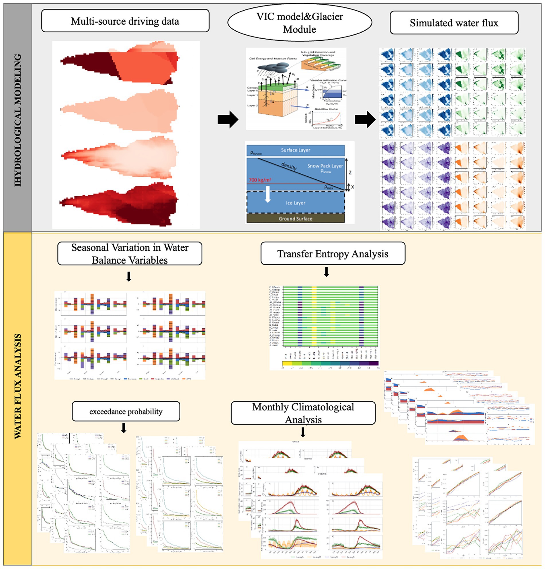
In this study, we proposed an information-theoretic framework to explore hydrological process connectivity under different meteorological forcing datasets and model configurations in a typical inland arid watershed. We employed the Variable Infiltration Capacity (VIC) model—enhanced with a glacier dynamics module—to simulate water fluxes in the Ebinur Lake Basin of northwestern China. Four different forcing datasets were used, including three station-based interpolation methods and one satellite-derived reanalysis product. To assess internal system interactions, we applied transfer entropy (TE) to quantify the directional and lagged information flows among key hydrological components, including precipitation, runoff, evapotranspiration, soil moisture, and snow water equivalent. This approach enabled us to move beyond conventional model evaluation and gain insights into the causal relationships and functional connectivity among subsystems under varying data and structural conditions (Figure 1).

Figure 1

Figure 1. Framework of hydrological modeling and water flux analysis.

2 Materials and methods

2.1 Materials

2.1.1 Study area

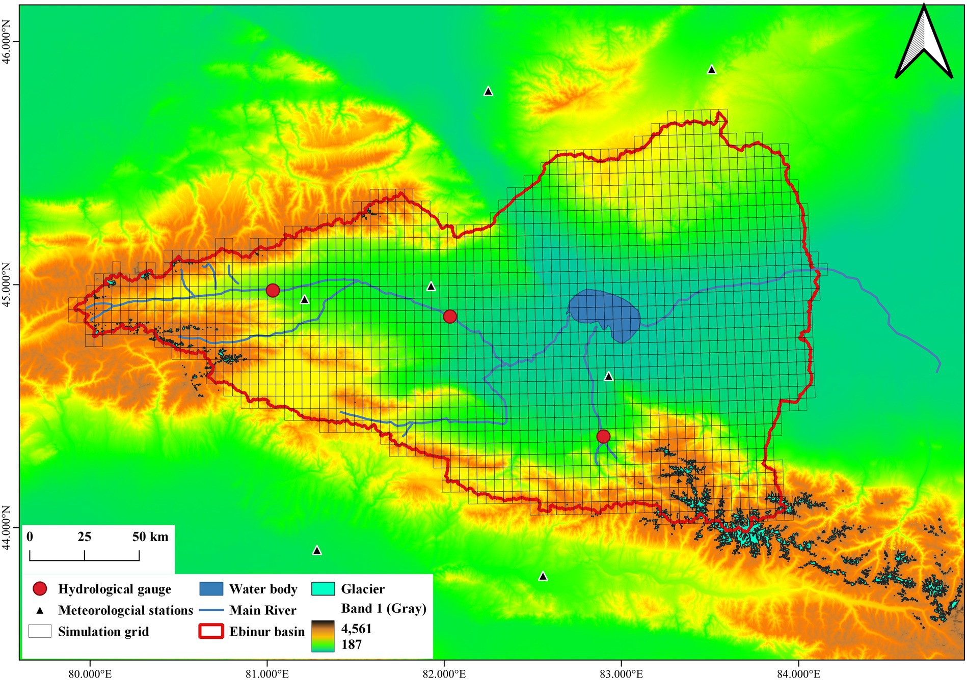
The Ebinur Lake Basin, located in the northwest of China’s Xinjiang Uyghur Autonomous Region, represents the lowest point of the Junggar Basin and contains Ebinur Lake—a large terminal saltwater lake (Figure 2; Wang et al., 2020). The basin’s primary inflows originate from the Bortala, Jing, and Kuitun Rivers, which rise in the Tianshan Mountains and define three distinct sub-basins (Zhang et al., 2023). The region is surrounded by mountains to the west, north, and south, forming a trumpet-shaped valley plain in the center that supports intensive agricultural activity (Bao et al., 2022). The basin experiences a typical inland arid climate, with an annual mean temperature of approximately 9°C. July and January are the hottest and coldest months, respectively. Annual precipitation ranges from 90 to 500 mm, while potential evapotranspiration reaches 1,500–3,400 mm (Wang Y. et al., 2021). Since the 1950s, extensive agricultural development and human interventions have significantly altered the regional hydrology. Currently, only the Jing and Bortala Rivers provide surface runoff recharge during the flood season, while most of the lake’s inflow originates from subsurface flow. As a result, Ebinur Lake has lost nearly 60% of its surface area compared to its extent in 1950 (Yushanjiang et al., 2018).

Figure 2

Figure 2. Study area map and distribution of simulation grids and observation sites.

2.1.2 Data

This study evaluates the influence of different meteorological data sources on simulated water fluxes in an inland arid basin, using three spatial interpolation methods—linear interpolation, inverse distance weighting (IDW), and thin plate spline (TPS)—alongside a satellite-based reanalysis dataset (Keller and Borkowski, 2019). All meteorological inputs were resampled to a uniform spatial resolution of 0.05° and a common temporal span of 2003–2017 for consistency in model simulations and comparative analysis (Table 1).

Table 1

Table 1. Summary of the four different meteorological driving data used in this study.

The IDW method estimates unknown grid cell values as weighted averages of surrounding stations based on geographic proximity. Linear interpolation fits straight-line segments between known data points, while TPS is a smoothing-based technique that incorporates covariate influences during spatial interpolation (Yoo, 2011). For TPS, WorldClim data were used as a climatic background field to reduce spatial bias in interpolation (Fick and Hijmans, 2017). The meteorological variables used as model forcing include daily maximum temperature, minimum temperature, wind speed, and precipitation.

Land surface inputs include soil and vegetation parameters from the VICGlobal dataset, and glacier extents derived from the Second Chinese Glacier Inventory (SCGI) (Schaperow et al., 2020; Sun M. et al., 2018). Observed streamflow records from three hydrological stations—Jinghe, Bole, and Wenquan—were obtained from the Ministry of Water Resources of China for the 2003–2017 period and used for simulation comparison and validation.

2.2 Methodology

2.2.1 Hydrologic model description

The hydrological simulations in this study were conducted using the Variable Infiltration Capacity (VIC) model, a semi-distributed, grid-based hydrologic framework designed to represent land surface–atmosphere interactions. The standard VIC model includes three primary submodules: (i) the water balance module, (ii) the energy balance module, and (iii) the snow and frozen soil module, which together allow the simulation of key surface and subsurface hydrological processes (Hamman et al., 2018). The soil water dynamics are represented by a three-layer conceptual structure: the top layer captures quick responses such as bare-soil evaporation from light rainfall; the middle layer models unsaturated water infiltration and root-zone processes; and the bottom layer simulates deep percolation and seasonal water retention. Subsurface runoff is computed using a conceptual ARNO baseflow formulation, while surface runoff results from excess infiltration based on a variable infiltration capacity curve. VIC explicitly simulates evapotranspiration (ET) as the sum of transpiration, canopy interception loss, and bare-soil evaporation, calculated using the Penman–Monteith method. Snow accumulation and melt are modeled using an energy balance approach with temperature thresholds to distinguish rain from snow, and frozen soil processes are also represented (Figure 3).

Figure 3

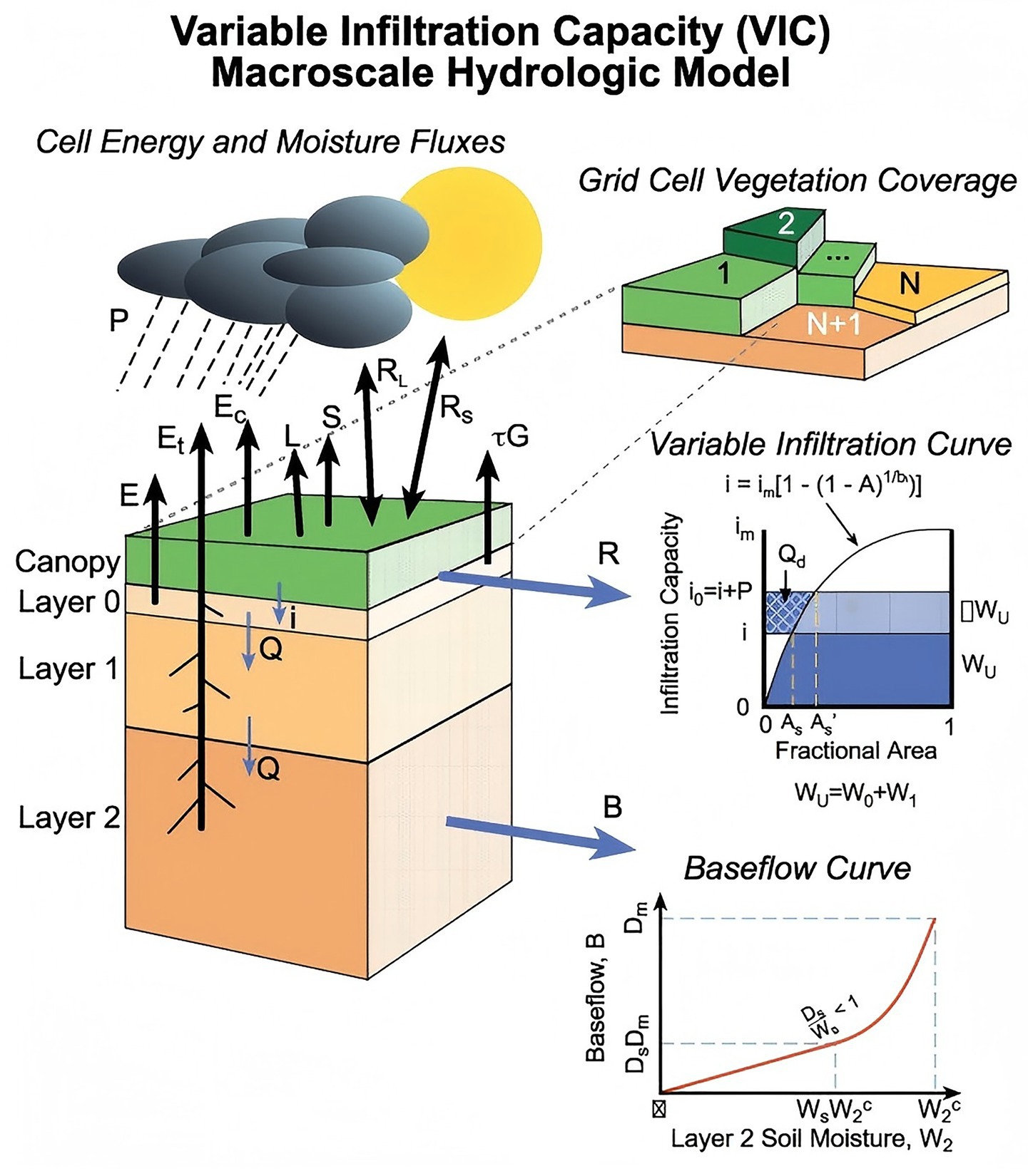
Figure 3. Schematic structure of the VIC model. Adapted from Hamman et al. (2018).

To account for land surface heterogeneity, VIC employs a sub-grid vegetation tiling scheme. Each grid cell is partitioned into multiple land cover classes, and water and energy fluxes are simulated separately for each vegetation tile (Scheidegger et al., 2021). The VIC model requires gridded meteorological forcing inputs—precipitation, maximum and minimum air temperature, and wind speed—along with land cover, vegetation, and soil parameters as input (Table 2).

Table 2

Table 2. VIC model parameter setup.

Since the standard VIC model does not account for glacier dynamics, this study incorporates a glacier module based on the scheme proposed by Joseph Hamman (Chegwidden et al., 2019). Glacier mass balance is simulated by adding an ice layer beneath the snowpack, using a density threshold of 750 kg/m³ to distinguish snow from ice. Snow density is assumed to increase linearly with depth. Glacier redistribution is modeled by applying a volume–area scaling relationship Bahr et al. (1997), and ablation is represented by integrating ice and snow layers into a unified melt calculation.

2.2.2 Information transfer entropy

Transfer entropy is mainly used to quantify the rate at which a stochastic or deterministic chaotic system evolves over time to produce information (Schreiber, 2000). In information theory, important insights into the structure of a system can be gained by individually measuring the components of the system to obtain contributions to information generation and how they exchange information with each other (Nearing and Gupta, 2015). The foundation of information theory was established by Shannon (1948), who defined the information entropy of a discrete random variable X with N possible outcomes as given by:

$\begin{array}{ll}{H}_x=-{\Sigma }_{\mathrm{i}=1}^N\rho \left(x_i\right)·{log}_{\mathit{\text{base}}}\rho \left(x_i\right)& (1)\end{array}$

where p(x_i) is the probability of occurrence of the outcome x_i and base is the base of the logarithm used (entropy has a binary numeric unit, bits, when base = 2).

Measuring the entropy between two random variables, called mutual information, can be thought of as the knowledge we gain about the other variable from measuring the source variable (Kraskov et al., 2004). But the mutual information between variables is symmetric, and it does not tell us the extent to which each variable contributes individually to the shared information. Schreiber (2000) derived an information-theoretic measure to quantify the evolution of a system over time, addressing the shortcoming that standard mutual information cannot distinguish between shared information, and this new method can effectively distinguish between drive and response elements and monitor asymmetries in subsystem interactions. This quantity of information transfer is called transfer entropy and has been known as a popular tool for estimating causal effects, time scales, and coupling strengths (Bennett et al., 2019). The formula for transfer entropy is given by.

$\begin{array}{ll}{T}_{X\to Y}(\tau ,\omega ,k,l)=I(Y_t;X_{t-\tau -k:t-\tau };Y_{t-\omega -l:t-\omega })& (2)\end{array}$

$\begin{array}{ll}{T}_{X\to Y}=I(Y_t;X_{t-1};Y_{t-1})& (3)\end{array}$

where $T_{X\to Y}$ denotes the entropy of the transfer from X to Y. Where parameters $k$ and $l$ represent the historical window sizes of the dependent and target variables, respectively, and $\tau$ and $\omega$ represent the time lags of the dependent and target goal variables, respectively. In this study, we set the parameters $\tau$ =1, $\omega$ =1, $k$ =0, $l$ =0, and choose the temporal resolution of the simulation as the method of choosing the time scale. The above 4 parameters are used to limit the complexity of high-dimensional calculations. The above equation enables the hydrological system under study to have the assumption of Markovian characteristics.

To make it easier to compute the probability distributions required for the information and entropy measures, this study uses the k-nearest-neighbor estimator in the nonparametric approach to estimating the distributions (Wang et al., 2006). Because of its advantages of general applicability and scalability, the estimators and parameters are chosen to minimize the average amount of deviation of each calculated information transfer. More details please refer to Bennett et al. (2019).

2.2.3 Water balance equation

This experimental simulation restricts all the variables analyzed to the water balance. Due to VIC model limitations, the simulated water fluxes do not include groundwater flow and grid lateral flow (Xia et al., 2018). We summarized the model output variables as precipitation (P), soil moisture (SM), runoff (R), evapotranspiration (ET), and snow water equivalent (SWE) according to the following equations.

$\begin{array}{ll}P=\mathit{ET}+R+\mathit{\text{ΔSWE}}+\mathit{\Delta SM}& (4)\end{array}$

where ET, P, and R are the average values, and the others are the variation values during the day. Defined as June to August for summer; September to November for fall; December, January, and February for winter; and March to May for spring, respectively. The transfer entropy was then calculated for each pair of variables on daily and monthly time scales, both using formulas with a time lag parameter of 1. In the discussion section, the changes in transfer entropy between hydrologic variables were calculated for different time lag parameters, thus observing the causality of their hydrologic subsystems coupled to each other. It is noted that Equation 4 does not explicitly include groundwater storage (GWS) due to the limitations of the standard VIC model, which does not simulate deep aquifer dynamics. Given the limited availability of groundwater data and the dominance of surface runoff in the upstream mountainous areas of the Ebinur Basin, we assumed that GWS variation was relatively minor over the simulation period.

3 Results

3.1 Spatiotemporal variation of hydrological variables

The spatial patterns of 15-year mean precipitation (2003–2017) driven by the four datasets exhibited notable differences (Supplementary Figure S1). Precipitation was generally concentrated along the mountainous periphery of the basin due to the orographic effect of the Tianshan Mountains. Interpolated products (A, A1, B) yielded lower overall precipitation than the satellite-derived dataset (C), with B showing smoother spatial transitions and an elevation-dependent gradient (Supplementary Figure S1b). In contrast, A1 produced more uniform spatial patterns that failed to capture topographic enhancements, while A showed fragmented spatial features (Supplementary Figures S1a,c). Although C captured general patterns, it significantly overestimated precipitation in the southern region. The TPS method used in B, supported by WorldClim as a climatic background, yielded more realistic spatial distributions overall.

Figure 4 presented the simulated mean annual evapotranspiration across different model configurations and forcing datasets. Evapotranspiration was more sensitive to the choice of forcing data than to model structural differences (e.g., glacier vs. frozen soil configurations). Forcings B and C consistently produced higher evapotranspiration values, with spatial peaks observed in the basin’s western and northeastern agricultural and desert fringe zones. Central regions around the tail lake exhibited lower values, likely due to the exclusion of lake/wetland components in the model. As shown in Figure 5, runoff simulations generally followed the spatial patterns of precipitation. Incorporating the glacier module led to more concentrated and intensified runoff in the western and southern mountainous areas, while differences across other model configurations (WATER, ENERGY, FROZEN) were relatively minor. Forcing A resulted in spatially fragmented runoff, while A1 produced uniformly low values. Unlike other cases, C-driven simulations exhibited runoff peaks in the central eastern basin. Simulated soil moisture exhibited clear spatial heterogeneity, with higher values concentrated around the basin margin and central regions. Forcings A and C yielded the highest soil moisture values but also showed significant spatial fragmentation, particularly for A. The B + FROZEN configuration produced inconsistent spatial patterns relative to other B-driven cases (Supplementary Figure S2). Finally, snow water equivalent exhibited consistent patterns, with high values predominantly located in the western and southern mountainous zones. Forcings C and A produced the highest snow accumulation, followed by B and A1 (Supplementary Figure S3).

Figure 4

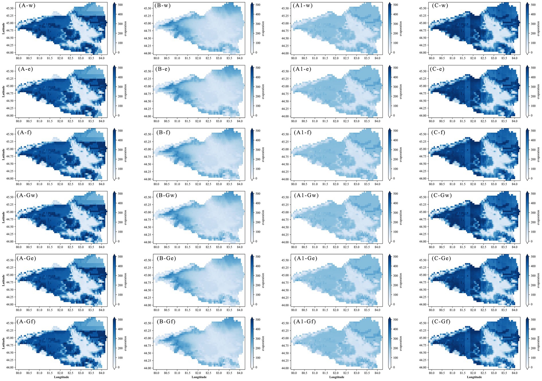
Figure 4. Mean annual evapotranspiration (mm) simulated using different combinations of meteorological forcing datasets (A, B, A1, C) and model configurations. Model configurations include water-only (w), energy balance (e), frozen soil (f), glacier + water (Gw), glacier + energy (Ge), and glacier + frozen soil (Gf).

Figure 5

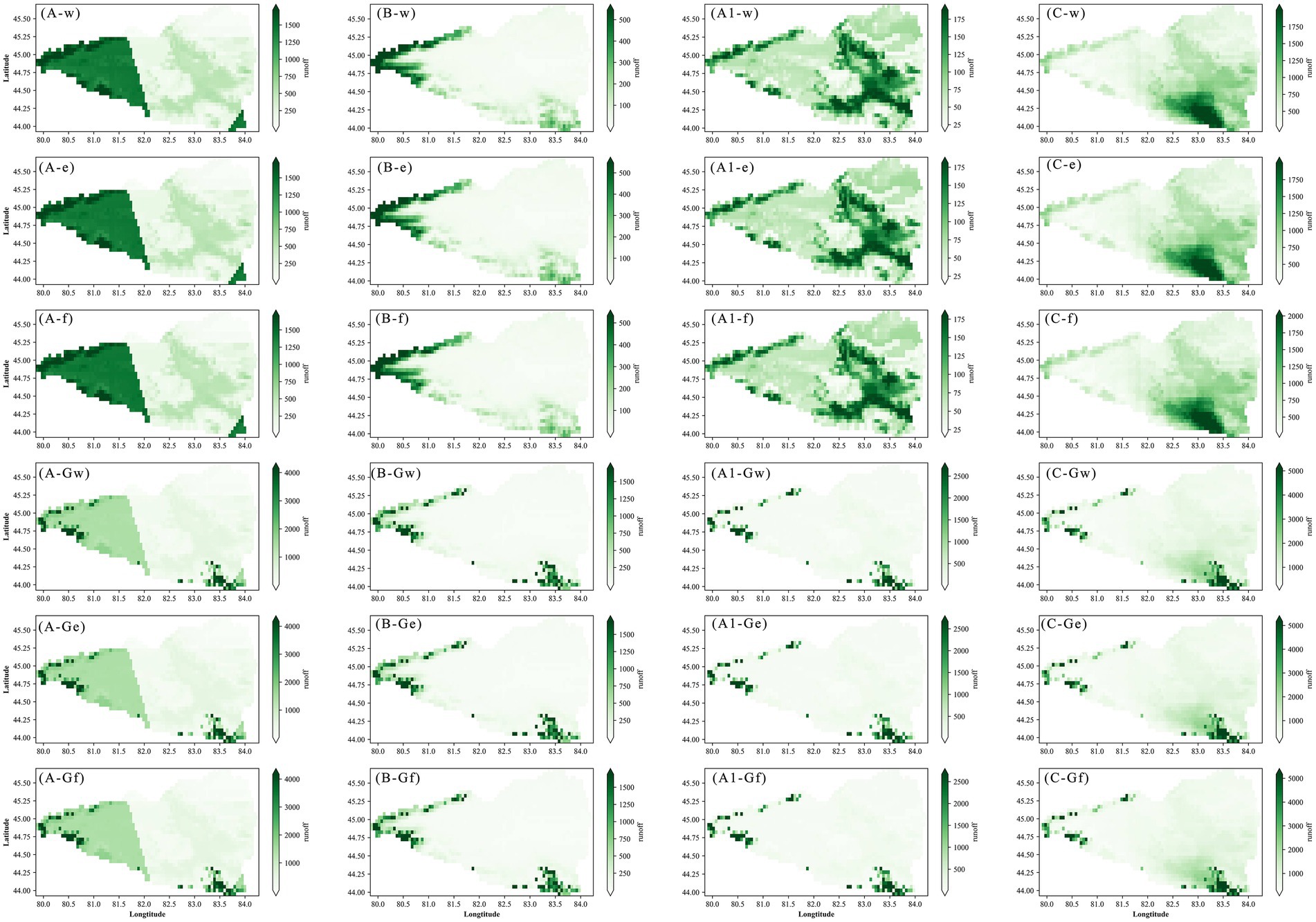
Figure 5. Mean annual runoff (mm) simulated under combinations of meteorological forcing datasets (A, B, A1, C) and model configurations. Model configurations include water-only (w), energy balance (e), frozen soil (f), glacier + water (Gw), glacier + energy (Ge), and glacier + frozen soil (Gf).

3.2 Seasonal variation in water balance variables

Figure 6 illustrated the seasonal water balance across all combinations of meteorological forcings and model configurations. All six model setups conserved water mass on an annual scale, although this was less evident in the monthly averaged time series plots. Substantial differences were observed in seasonal flux magnitudes among the various driver–model combinations, highlighting the sensitivity of simulated water balances to both input data and model structure. Notably, driver A1 consistently produced the lowest summer fluxes across most model configurations. The largest inter-model variability occurred in evapotranspiration (ET) and soil moisture (SM), particularly during warm seasons.

Figure 6

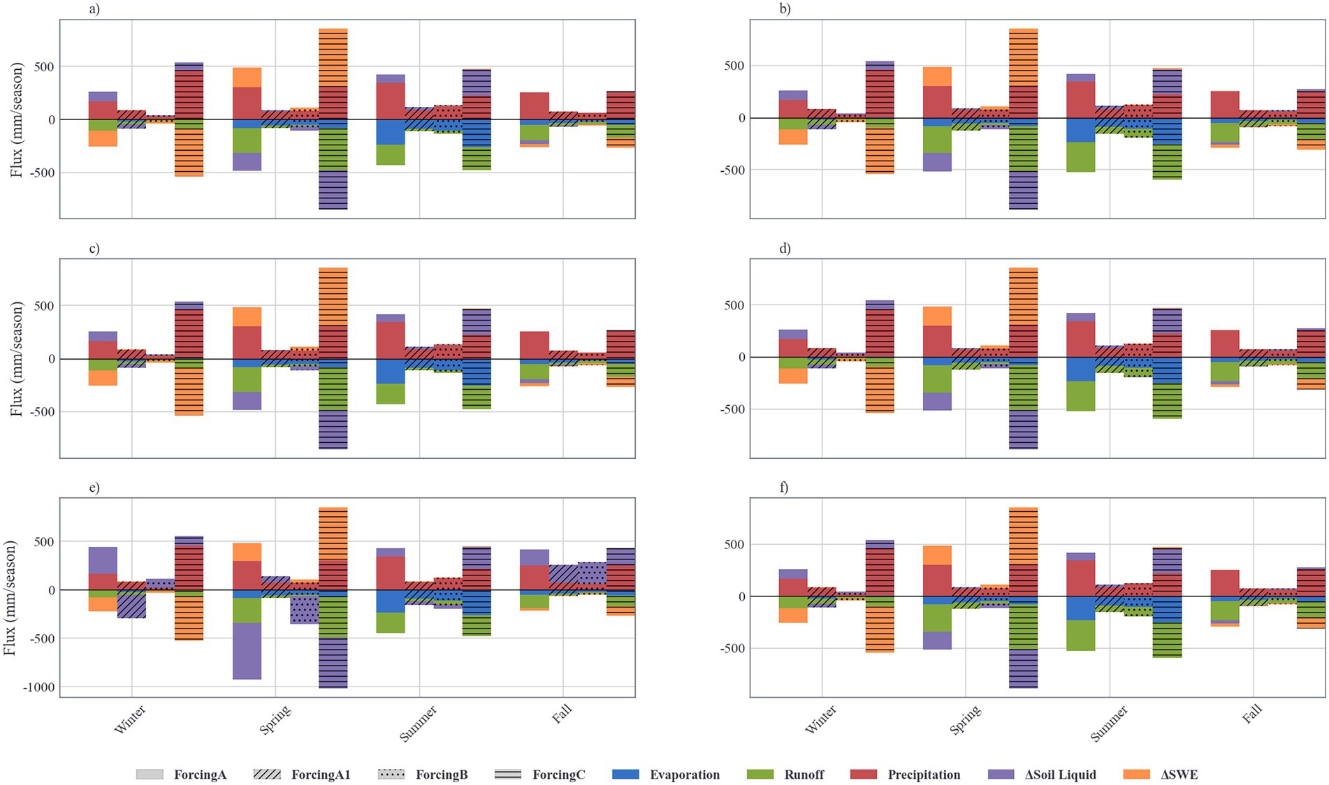
Figure 6. Seasonal water balance simulated under four meteorological forcing datasets across six model configurations. Subfigures represent: (a) WATER; (b) G-WATER; (c) ENERGY; (d) G-ENERGY; (e) FROZEN; and (f) G-FROZEN configurations.

In the FROZEN model configuration without glacier components, combinations using forcings A, A1, and B exhibited seasonal imbalances in water fluxes, likely due to temperature-driven soil moisture–freeze–thaw interactions. Similar inconsistencies were identified in the G-FROZEN setup, though to a lesser extent. These anomalies suggested that the frozen soil module’s melting mechanism inadequately coupled temperature and soil moisture dynamics. In contrast, the remaining model setups exhibited more stable seasonal behavior. Among all forcing datasets, driver C consistently generated the highest seasonal water fluxes, followed by A and A1.

To further quantify seasonal hydrological responses, the runoff ratio (R/P) was calculated for each scenario (Table 3). Driver datasets B and A1 produced the lowest runoff ratios across model sets, reflecting their lower precipitation inputs. Conversely, driver C yielded the highest runoff ratios in all configurations, suggesting a stronger precipitation–runoff coupling. These seasonal differences in flux partitioning provided the basis for the subsequent analysis of causal interactions among hydrological components using transfer entropy.

Table 3

Table 3. Runoff Ratio (R/P) was calculated and simulated for each model and driving data.

3.3 Hydrological variables monthly climatological analysis

Figure 7 and Supplementary Figures 4, 5 depict the monthly climatology of four key hydrological variables—ET, SWE, runoff, and soil moisture—across six model configurations and four meteorological forcings from 2003 to 2017. All variables are represented using daily medians and interquartile ranges to reflect variability. Evapotranspiration (ET) showed distinct seasonal behavior, peaking between May and August. Forcing C yielded the highest ET values (up to ~3 mm/day), while forcing B remained the lowest (mostly <1.2 mm/day). Forcing A1 displayed strong winter–spring oscillations due to early snowmelt, but glacier inclusion had minimal impact on ET seasonality.

Figure 7

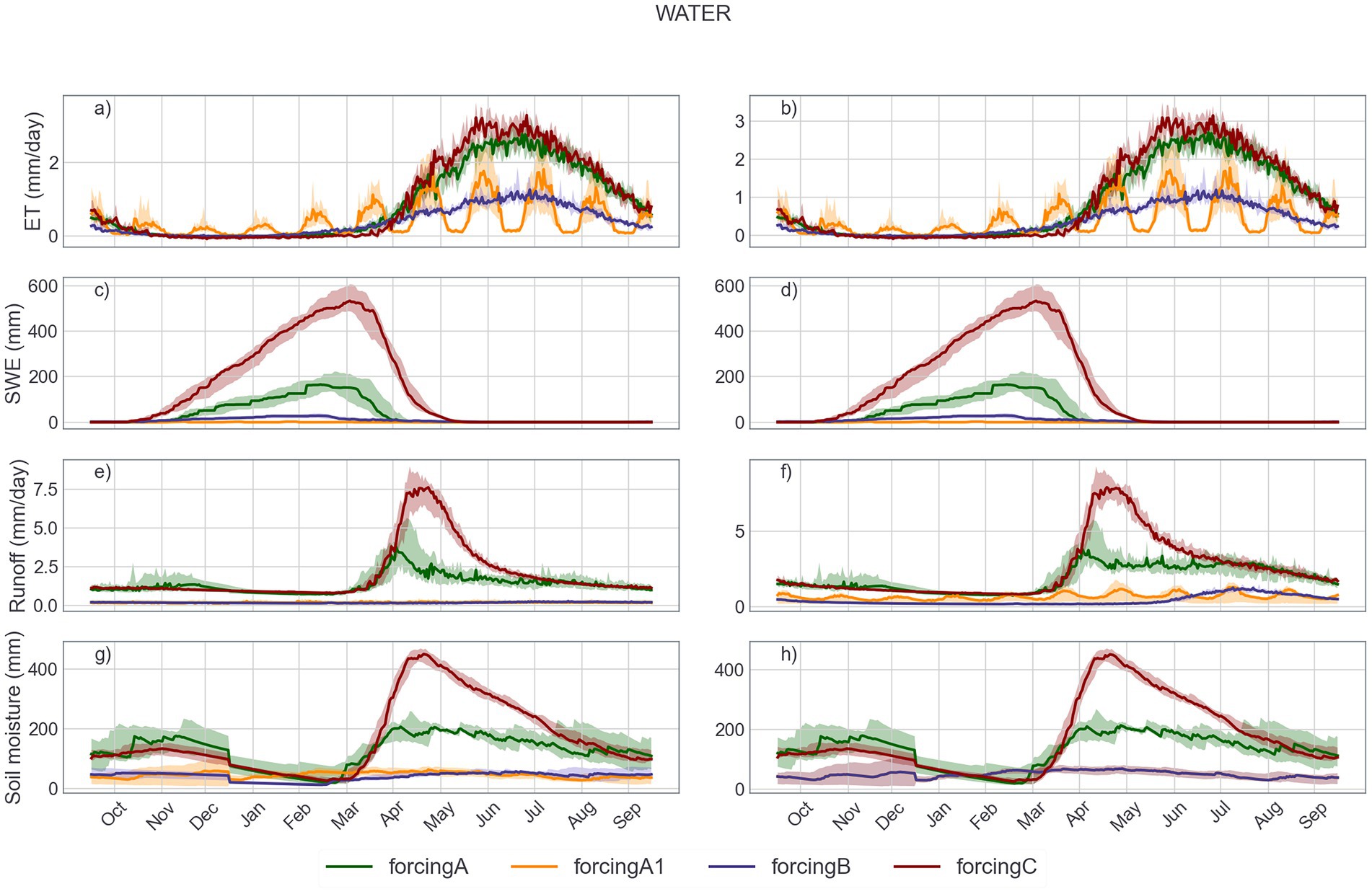
Figure 7. Monthly evolution of key hydrological variables under four meteorological forcings (A, A1, B, and C) in two model configurations. Panels a, c, e, and g represent the WATER configuration, while panels b, d, f, and h represent the FROZEN configuration. Variables include (a,b) evapotranspiration (ET), (c,d) snow water equivalent (SWE), (e,f) runoff, and (g,h) soil moisture. Solid lines indicate the daily median values, and the shaded areas represent interquartile ranges over the simulation period. Forcing C generally produces the highest SWE and runoff, while A1 yields the lowest across variables.

Snow Water Equivalent (SWE) under forcing C reached a peak of ~580 mm in late March, significantly higher than A (~350 mm) and B/A1 (<100 mm). Glacier modules had limited effect on SWE magnitude or timing, suggesting dominant control by input precipitation and temperature. Runoff patterns were closely tied to SWE and ET trends. Forcing C generated the highest spring runoff (~6.5 mm/day in April), followed by A (~3.8 mm/day), with B and A1 mostly <2 mm/day. Glacier inclusion notably increased A1 runoff by over 60% during melt periods. Forcing B produced a secondary summer peak (~2 mm/day in July), indicating delayed snowmelt. Soil moisture under forcing C peaked in May–June (~380 mm), ~1.5–2 times higher than A and B. A1 and B exhibited relatively flat profiles (~180–220 mm), with minor seasonal fluctuation. Enabling glacier modules slightly enhanced spring soil moisture in A1 and B but had limited effect in other cases. Overall, forcing C consistently produced higher water availability, while B and A1 showed muted responses under both WATER and G-WATER setups.

3.4 Transfer entropy analysis

Figure 8 presented the simulated one-day lagged transfer entropy (TE) between hydrological components under all combinations of meteorological forcing and model configurations. These values, averaged over the 15-year simulation period, revealed the structure of information exchange networks across the water year in the Ebinur Basin.

Figure 8

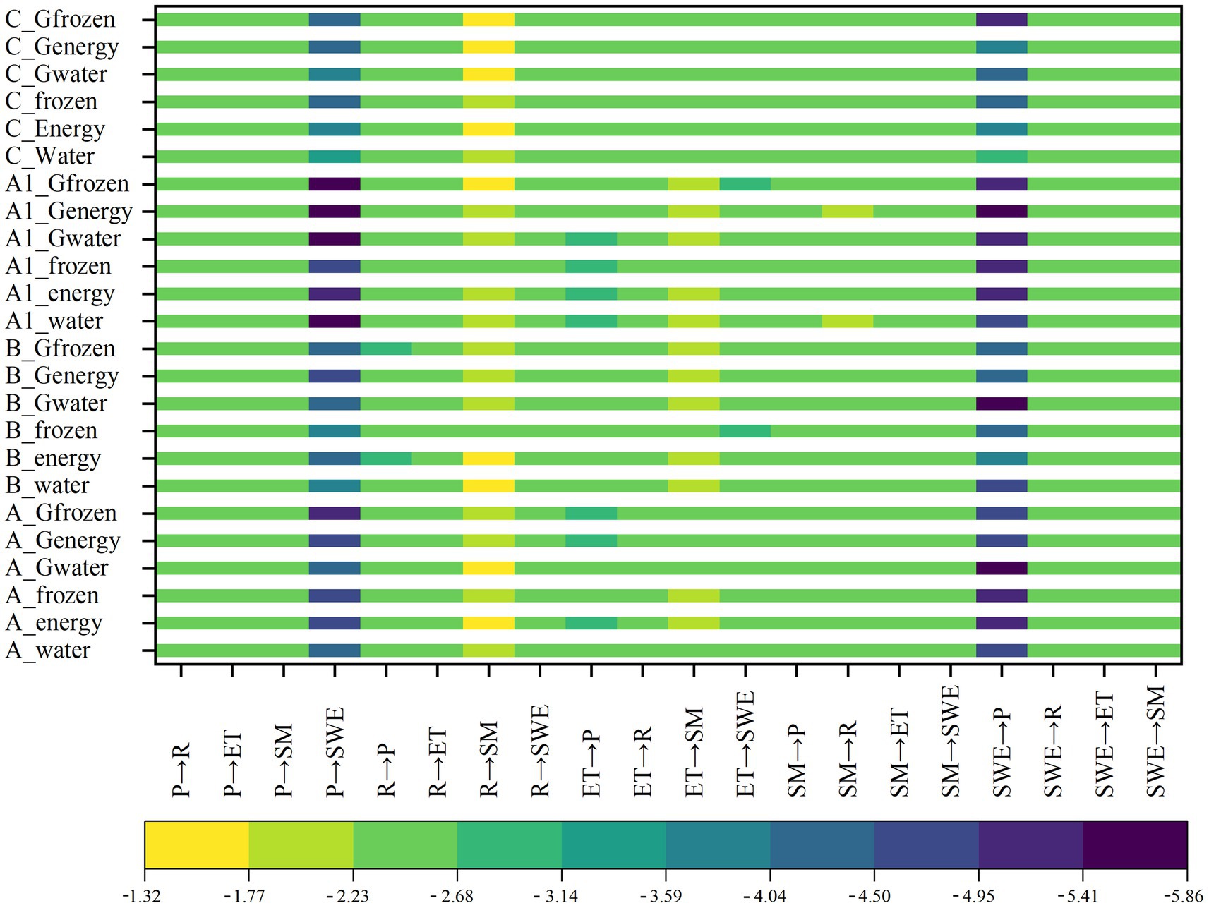
Figure 8. One-day lagged transfer entropy matrix among major hydrological variables (P: precipitation, R: runoff, ET: evapotranspiration, SM: soil moisture, SWE: snow water equivalent) in the Ebinur Lake Basin under different model structures and meteorological forcing datasets. Model categories are grouped first by forcing dataset (A, A1, B, C), and then by model configuration: WATER (water balance), ENERGY (energy balance), FROZEN (with frozen soil processes), G-WATER, G-ENERGY, and G-FROZEN (glacier-enhanced versions). The color intensity represents the magnitude of normalized transfer entropy (TE) from the row variable (source) to the column variable (target). Warmer colors indicate stronger directed information flow. Transfer entropy values were log-transformed and normalized, resulting in unitless magnitudes represented by color gradients. The original TE values were computed in bits (log₂ base).

Runoff (R) and evapotranspiration (ET) consistently exhibited the strongest information transfer to other variables across all combinations, reflecting their central role in the hydrological process network. In contrast, the TE from precipitation (P) to snow water equivalent (SWE) was consistently the lowest, suggesting weak direct coupling. This was attributed to the model structure, where the influence of precipitation on SWE was mediated through intermediate processes such as temperature or snowmelt rather than direct accumulation. The lowest TE values for P → SWE were observed under the A1 forcing with glacier model configurations, particularly A1_Gfrozen. A similar pattern was found in the reverse direction (SWE → P), with TE values typically below −4.40. TE values among R, ET, and soil moisture (SM) were generally higher (ranging from −2.23 to −3.59), indicating strong bidirectional interactions and efficient information exchange within these subsystems. Notably, TE from R to SM under C and A forcings showed elevated values. In contrast, TE from ET to P was lowest in combinations such as A1_Gwater, A1_frozen, A1_energy, A1_water, and several A-based non-glacier configurations. Higher TE values from ET to SM were concentrated in combinations involving glacier-enhanced model configurations under A1 and B forcings. Meanwhile, TE from ET to SWE was relatively uniform across combinations, with the lowest values found in A1_Genergy and A1_water. The heatmap visualization enabled a clear comparative assessment of information transfer dynamics, supporting an improved understanding of subsystem coupling strength and highlighting the role of specific driver–model pairings in shaping hydrological connectivity.

4 Discussion

4.1 Comparison of transfer entropy and correlation of each hydrological variable to runoff

To better understand the hydrological controls on runoff beyond average runoff ratios (e.g., lower values under forcing B in Table 3), we evaluated both lagged transfer entropy (TE) and Pearson correlation between monthly runoff and other key variables (precipitation, SWE, soil moisture, and ET) under all model configurations and meteorological forcings.

Seasonal patterns of TE were distinct. In spring (March–May), TE values increased sharply across all forcing-model combinations, driven by snowmelt contributions. For example, SWE showed peak TE to runoff in April–May under forcing C, while soil moisture became informative under A1 and C in late spring. Outside of spring, particularly in autumn and winter, TE from precipitation to runoff diminished significantly under B and C, indicating that runoff was more strongly influenced by lagged processes such as subsurface flow or snowmelt-driven soil water rather than direct rainfall.

Correlation patterns further revealed forcing-dependent behaviors. Under forcing C, precipitation was negatively correlated with runoff from April to August (r ≈ −0.3 to −0.5), whereas SWE maintained strong positive correlations in summer (r ≈ 0.6) and autumn (r ≈ 0.4). ET showed a positive correlation with runoff in spring (e.g., r > 0.5 under A and C), but shifted to negative values in winter under A and B. Notably, A1 exhibited the weakest and least consistent correlations across variables, yet TE analysis suggested hidden nonlinear dependencies—especially for ET and SWE in autumn—underscoring the complementarity of TE over linear correlation methods.

The spatial interpolation method used in forcing data influenced the strength and stability of information flow. Satellite-driven forcing (C) yielded the most coherent patterns in both TE and correlation, while interpolation-based forcings (A, B, A1) displayed fragmented or inconsistent signal transfer. Among them, IDW provided relatively stable monthly TE trends, TPS showed good alignment with C but with generally lower TE magnitudes, and linear interpolation performed most erratically.

Across all VIC model variants—including those with activated glacier components—the patterns of TE and correlation remained broadly consistent, suggesting that the meteorological forcing exerts greater control on runoff information dynamics than structural model complexity (Figure 9).

Figure 9

Figure 9. Monthly dynamics of hydrological variables’ influence on runoff in the WATER model configuration under four forcing datasets (A, A1, B, C). (a) One-day lagged normalized transfer entropy from each variable—precipitation (P), evapotranspiration (ET), soil moisture (SM), and snow water equivalent (SWE)—to runoff, highlighting the strength of directed information transfer. (b) Pearson correlation coefficients between the same variables and runoff, capturing linear relationships over time. Each panel corresponds to a specific forcing dataset. Color bands represent different variables (see legend), and the x-axis spans the hydrological year from October to September. The comparison reveals distinct temporal and structural patterns in both causal and correlative relationships across datasets.

4.2 Explain the relationship between subsystems using information transfer theory

Transfer entropy (TE) provides a directional, lag-sensitive metric to quantify the information flow between system components, effectively distinguishing dynamic interactions from static correlations caused by shared inputs or system memory (Konapala et al., 2020). To assess process-level connectivity in hydrological subsystems, we computed TE across varying lag steps for different model configurations and meteorological forcing datasets (Figure 10; Supplementary Figures 11, 12).

Figure 10

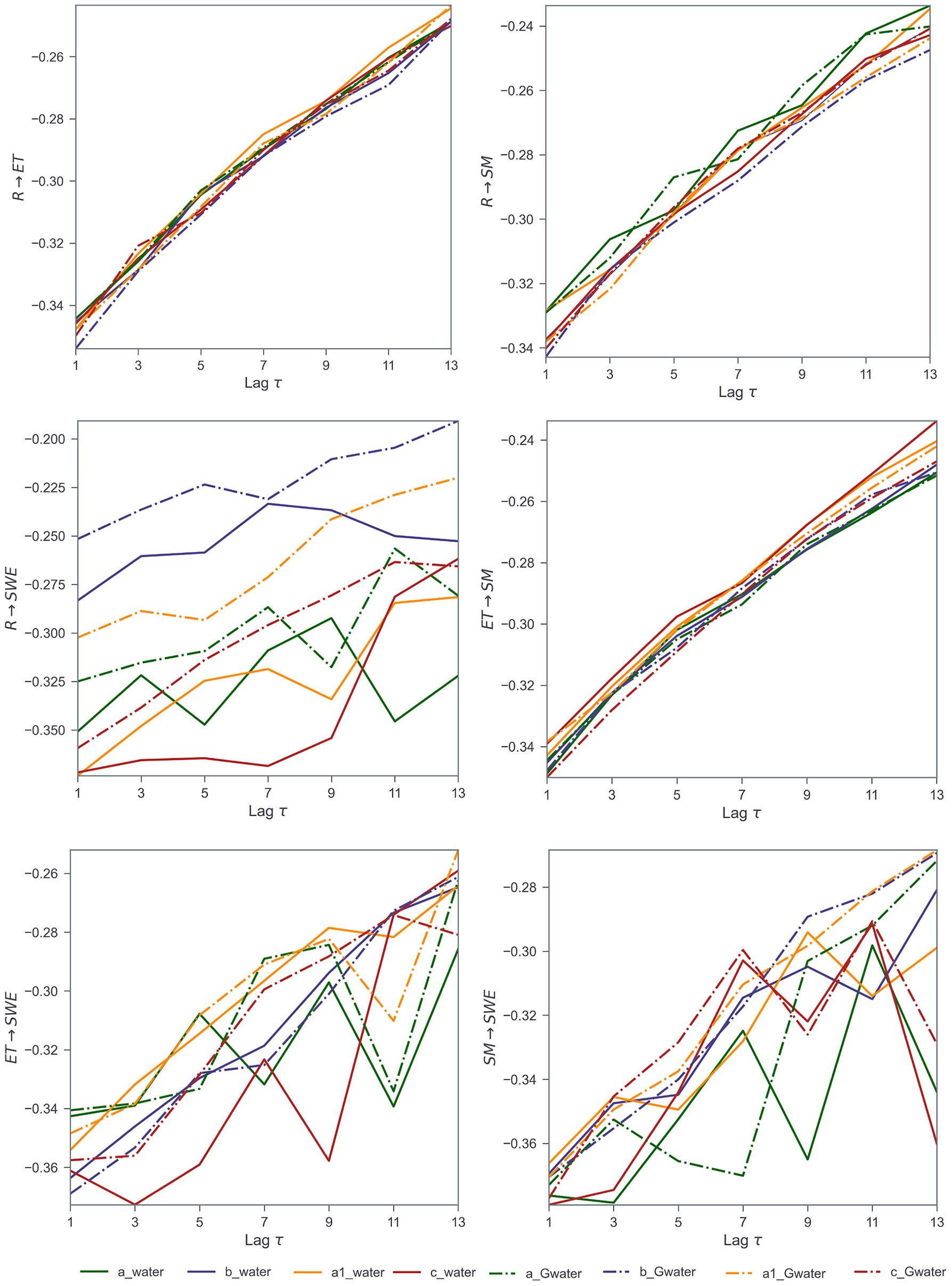
Figure 10. Effects of increasing lag steps (τ) on transfer entropy between key hydrological variables in the WATER and G-WATER model configurations. Each panel represents a pairwise information flow direction: (R → ET): runoff to evapotranspiration; (R → SM): runoff to soil moisture; (R → SWE): runoff to snow water equivalent; (ET → SM): evapotranspiration to soil moisture; (ET → SWE): evapotranspiration to snow water equivalent; (SM → SWE): soil moisture to snow water equivalent. Lines indicate the strength of one-day to 13-day lagged transfer entropy, comparing four different meteorological forcings (A, B, A1, C) applied to two configurations: Solid lines: WATER (standard model); Dash-dotted lines: G-WATER (glacier-enhanced model). Colors represent different forcing datasets: Blue = A; Purple = B; Orange = A1; Red = C. This figure highlights how lag-dependent causal interactions vary across meteorological inputs and model structures. G-WATER configurations generally show higher TE persistence in snow-dominated processes, especially for SWE-related pathways.

In the water balance model sets, including glacier-enhanced versions, TE from runoff (R) to evapotranspiration (ET) and from R to soil moisture (SM) showed clear linear increases with increasing lag steps—indicating stable and direct causal relationships. Exceptions were observed in the a_water and a_Gwater configurations, which exhibited irregular R → SM patterns. In contrast, TE from R to snow water equivalent (SWE) displayed more fluctuation, particularly under b_water and b_Gwater, where values were higher but less stable. Similar trends were observed in the energy and frozen soil model sets, reinforcing the finding that R → ET and R → SM represented consistent and strong information pathways across the VIC model structure. Additionally, TE from ET to SM exhibited a regular, lag-dependent increase across all configurations, suggesting a robust bidirectional coupling between these subsystems. Conversely, TE between ET and SWE, as well as SM and SWE, showed irregular or flat patterns, indicating weak or indirect interactions. These results suggested that SWE did not maintain stable causal linkages with ET or SM in the model structure.

Overall, the findings aligned with prior studies in arid regions (Chen et al., 2020; Li et al., 2018; Wang et al., 2017), confirming that runoff, evapotranspiration, and soil moisture are closely interconnected, while SWE remains more loosely coupled. Our use of transfer entropy within a physically based hydrological model enabled a nuanced quantification of subsystem interactions beyond traditional correlation methods.

5 Conclusion

This study explored the hydrological impacts of different meteorological forcing datasets—three station-based interpolation methods and one satellite reanalysis dataset—combined with multiple VIC model configurations, including glacier and permafrost modules. Spatial and seasonal patterns of hydrological fluxes were assessed, and the coupling relationships among subsystems were further evaluated using transfer entropy.

The results demonstrated that satellite reanalysis data (forcing C) provided more spatially consistent representations of precipitation than station-based interpolation, leading to more coherent simulations of other hydrological fluxes. In seasonal water balance analysis, precipitation and snow water equivalent dominated in winter and spring, while runoff and evapotranspiration were more prominent in summer and autumn. Notably, the permafrost model configuration exhibited seasonal imbalances, particularly in autumn and winter.

Transfer entropy revealed nuanced, lag-dependent causal relationships among hydrological subsystems. The strongest information transfer occurred between runoff and soil moisture, and between evapotranspiration and soil moisture, indicating stable bidirectional interactions. In contrast, the weakest information transfer was observed between precipitation and snow water equivalent, suggesting a more indirect linkage. Compared with traditional correlation analysis, transfer entropy more effectively captured the directionality and time-lagged dynamics of water flux interactions.

This work highlighted the value of integrating multi-source meteorological data with information-theoretic approaches to better understand process connectivity within complex hydrological models. Future research should further explore data fusion strategies combining remote sensing and in-situ observations, especially in data-sparse and cryospheric regions. The use of transfer entropy under different driving scenarios offers a promising path for diagnosing and improving the internal consistency of large-scale hydrological modeling systems.

Data availability statement

Publicly available datasets were analyzed in this study. This data can be found at: Meteorological and remote sensing datasets are publicly available from the National Tibetan Plateau Data Center: https://data.tpdc.ac.cn/en/. Glacier data were retrieved from the Second Chinese Glacier Inventory, available at the National Tibetan Plateau Data Center: https://data.tpdc.ac.cn/en/data/f92a4346-a33f-497d-9470-2b357ccb4246. The VIC model is available at: https://github.com/UW-Hydro/VIC.

Author contributions

QB: Project administration, Visualization, Methodology, Supervision, Validation, Data curation, Formal analysis, Conceptualization, Software, Funding acquisition, Writing – review & editing, Resources, Investigation, Writing – original draft. LZ: Data curation, Formal analysis, Visualization, Writing – review & editing. JT: Software, Methodology, Writing – review & editing.

Funding

The author(s) declare that financial support was received for the research and/or publication of this article. This research was supported by the Xinjiang Uygur Autonomous Region Philosophy and Social Science Foundation (Grant No. 2025CTJ065), the Basic Research Program for Universities in Xinjiang Uygur Autonomous Region (Grant No. XJEDU2025J114), and the High-level Talent Recruitment Project of Xinjiang University of Finance and Economics (Grant No. 40031388). The author gratefully acknowledges the institutional support provided throughout the course of this study.

Conflict of interest

The authors declare that the research was conducted in the absence of any commercial or financial relationships that could be construed as a potential conflict of interest.

Generative AI statement

The authors declare that no Gen AI was used in the creation of this manuscript.

Any alternative text (alt text) provided alongside figures in this article has been generated by Frontiers with the support of artificial intelligence and reasonable efforts have been made to ensure accuracy, including review by the authors wherever possible. If you identify any issues, please contact us.

Publisher’s note

All claims expressed in this article are solely those of the authors and do not necessarily represent those of their affiliated organizations, or those of the publisher, the editors and the reviewers. Any product that may be evaluated in this article, or claim that may be made by its manufacturer, is not guaranteed or endorsed by the publisher.

Supplementary material

The Supplementary material for this article can be found online at: https://www.frontiersin.org/articles/10.3389/frwa.2025.1622980/full#supplementary-material

References

Bahr, D. B., Meier, M. F., and Peckham, S. D. (1997). The physical basis of glacier volume-area scaling. J. Geophys. Res. Solid Earth 102, 20355–20362. doi: 10.1029/97JB01696

Crossref Full Text | Google Scholar

Bao, Q., Ding, J., Han, L., Li, J., and Ge, X. (2022). Predicting land change trends and water consumption in typical arid regions using multi-models and multiple perspectives. Ecol. Indic. 141:109110. doi: 10.1016/j.ecolind.2022.109110

Crossref Full Text | Google Scholar

Bennett, A., Nijssen, B., Ou, G., Clark, M., and Nearing, G. (2019). Quantifying process connectivity with transfer entropy in hydrologic models. Water Resour. Res. 55, 4613–4629. doi: 10.1029/2018WR024555

Crossref Full Text | Google Scholar

Chegwidden, O. S., Nijssen, B., Rupp, D. E., Arnold, J. R., Clark, M. P., Hamman, J. J., et al. (2019). How do modeling decisions affect the spread among hydrologic climate change projections? Exploring a large ensemble of simulations across a diversity of hydroclimates. Earths Future 7, 623–637. doi: 10.1029/2018EF001047

Crossref Full Text | Google Scholar

Chen, Y., Zhang, X., Fang, G., Li, Z., Wang, F., Qin, J., et al. (2020). Potential risks and challenges of climate change in the arid region of northwestern China. Reg. Sustain. 1, 20–30. doi: 10.1016/j.regsus.2020.06.003

Crossref Full Text | Google Scholar

Fick, S. E., and Hijmans, R. J. (2017). Worldclim 2: new 1-km spatial resolution climate surfaces for global land areas. Int. J. Climatol. 37, 4302–4315. doi: 10.1002/joc.5086

Crossref Full Text | Google Scholar

Franzen, S. E., Farahani, M. A., and Goodwell, A. E. (2020). Information flows: characterizing precipitation-streamflow dependencies in the Colorado headwaters with an information theory approach. Water Resour. Res. 56:e2019wr026133. doi: 10.1029/2019WR026133

Crossref Full Text | Google Scholar

Guo, B., Xu, T., Zhang, J., Croke, B., Jakeman, A., Seo, L., et al. (2017). A comparative analysis of precipitation estimation methods for streamflow prediction. Hobart, Tasmania, Australia: Presented at the 22nd International Congress on Modelling and Simulation (MODSIM2017). 3–8.

Google Scholar

Guo, B., Zhang, J., Xu, T., Croke, B., Jakeman, A., Song, Y., et al. (2018). Applicability assessment and uncertainty analysis of multi-precipitation datasets for the simulation of hydrologic models. Water 10:1611. doi: 10.3390/w10111611

Crossref Full Text | Google Scholar

Guo, B., Zhang, J., Xu, T., Song, Y., Liu, M., and Dai, Z. (2022). Assessment of multiple precipitation interpolation methods and uncertainty analysis of hydrological models in Chaohe River basin, China. Water SA 48, 324–334. doi: 10.17159/wsa/2022.v48.i3.3884

Crossref Full Text | Google Scholar

Hadjimichael, A., Yoon, J., Reed, P., Voisin, N., and Xu, W. (2023). Exploring the consistency of water scarcity inferences between large-scale hydrologic and node-based water system model representations of the upper Colorado River basin. J. Water Resour. Plan. Manag. 149:04022081. doi: 10.1061/JWRMD5.WRENG-5522

Crossref Full Text | Google Scholar

Hamman, J. J., Nijssen, B., Bohn, T. J., Gergel, D. R., and Mao, Y. (2018). The variable infiltration capacity model version 5 (Vic-5): infrastructure improvements for new applications and reproducibility. Geosci. Model Dev. 11, 3481–3496. doi: 10.5194/gmd-11-3481-2018

Crossref Full Text | Google Scholar

Keller, W., and Borkowski, A. (2019). Thin plate spline interpolation. J. Geod. 93, 1251–1269. doi: 10.1007/s00190-019-01240-2

Crossref Full Text | Google Scholar

Konapala, G., Kao, S. C., and Addor, N. (2020). Exploring hydrologic model process connectivity at the continental scale through an information theory approach. Water Resour. Res. 56:e2020wr027340. doi: 10.1029/2020WR027340

Crossref Full Text | Google Scholar

Kraskov, A., Stögbauer, H., and Grassberger, P. (2004). Estimating mutual information. Phys. Rev. E 69:066138. doi: 10.1103/PhysRevE.69.066138

PubMed Abstract | Crossref Full Text | Google Scholar

Kumar, P., and Gupta, H. V. (2020). Debates—does information theory provide a new paradigm for earth science? Wiley online library. Water Resour. Res. 56. doi: 10.1029/2019WR026398

Crossref Full Text | Google Scholar

Li, X., Cheng, G., Ge, Y., Li, H., Han, F., Hu, X., et al. (2018). Hydrological cycle in the Heihe River basin and its implication for water resource management in endorheic basins. J. Geophys. Res. Atmos. 123, 890–914. doi: 10.1002/2017JD027889

Crossref Full Text | Google Scholar

Liu, X., Yang, K., Ferreira, V. G., and Bai, P. (2022). Hydrologic model calibration with remote sensing data products in global large basins. Water Resour. Res. :e2022wr032929. doi: 10.1029/2022WR032929

Crossref Full Text | Google Scholar

Mendoza, P. A., Clark, M. P., Mizukami, N., Newman, A. J., Barlage, M., Gutmann, E. D., et al. (2015). Effects of hydrologic model choice and calibration on the portrayal of climate change impacts. J. Hydrometeorol. 16, 762–780. doi: 10.1175/JHM-D-14-0104.1

Crossref Full Text | Google Scholar

Moges, E., Demissie, Y., Larsen, L., and Yassin, F. (2021). Sources of hydrological model uncertainties and advances in their analysis. Water 13:28. doi: 10.3390/w13010028

Crossref Full Text | Google Scholar

Nearing, G. S., and Gupta, H. V. (2015). The quantity and quality of information in hydrologic models. Water Resour. Res. 51, 524–538. doi: 10.1002/2014WR015895

Crossref Full Text | Google Scholar

Nearing, G. S., Tian, Y., Gupta, H. V., Clark, M. P., Harrison, K. W., and Weijs, S. V. (2016). A philosophical basis for hydrological uncertainty. Hydrol. Sci. J. 61, 1666–1678. doi: 10.1080/02626667.2016.1183009

Crossref Full Text | Google Scholar

Pandi, D., Kothandaraman, S., and Kuppusamy, M. (2021). Hydrological models: a review. Int. J. Hydrol. Sci. Technol. 12, 223–242. doi: 10.1504/IJHST.2021.117540

Crossref Full Text | Google Scholar

Ruddell, B. L., Drewry, D. T., and Nearing, G. S. (2019). Information theory for model diagnostics: structural error is indicated by trade-off between functional and predictive performance. Water Resour. Res. 55, 6534–6554. doi: 10.1029/2018WR023692

Crossref Full Text | Google Scholar

Schaperow, J., Li, D., Margulis, S. A., and Lettenmaier, D. P. (2020). Vicglobal: a globally consistent setup for the variable infiltration capacity model. Agu Fall Meeting Abstracts :H201-01.

Google Scholar

Scheidegger, J. M., Jackson, C. R., Muddu, S., Tomer, S. K., and Filgueira, R. (2021). Integration of 2D lateral groundwater flow into the variable infiltration capacity (Vic) model and effects on simulated fluxes for different grid resolutions and aquifer diffusivities. Water 13:663. doi: 10.3390/w13050663

Crossref Full Text | Google Scholar

Schreiber, T. (2000). Measuring information transfer. Phys. Rev. Lett. 85, 461–464. doi: 10.1103/PhysRevLett.85.461

PubMed Abstract | Crossref Full Text | Google Scholar

Schreiner-Mcgraw, A. P., and Ajami, H. (2020). Impact of uncertainty in precipitation forcing data sets on the hydrologic budget of an integrated hydrologic model in mountainous terrain. Water Resour. Res. 56:e2020wr027639. doi: 10.1029/2020WR027639

Crossref Full Text | Google Scholar

Shannon, C. E. (1948). A mathematical theory of communication. Bell Syst. Tech. J. 27, 379–423. doi: 10.1002/j.1538-7305.1948.tb01338.x

Crossref Full Text | Google Scholar

Sun, M., Liu, S., Yao, X., Guo, W., and Xu, J. (2018). Glacier changes in the Qilian Mountains in the past half-century: based on the revised first and second Chinese glacier inventory. J. Geogr. Sci. 28, 206–220. doi: 10.1007/s11442-018-1468-y

Crossref Full Text | Google Scholar

Sun, R., Yuan, H., Liu, X., and Jiang, X. (2016). Evaluation of the latest satellite–gauge precipitation products and their hydrologic applications over the Huaihe River basin. J. Hydrol. 536, 302–319. doi: 10.1016/j.jhydrol.2016.02.054

Crossref Full Text | Google Scholar

Sun, R., Yuan, H., and Yang, Y. (2018). Using multiple satellite-gauge merged precipitation products ensemble for hydrologic uncertainty analysis over the Huaihe River basin. J. Hydrol. 566, 406–420. doi: 10.1016/j.jhydrol.2018.09.024

Crossref Full Text | Google Scholar

Tan, M. L., and Santo, H. (2018). Comparison of Gpm Imerg, Tmpa 3B42 and Persiann-Cdr satellite precipitation products over Malaysia. Atmos. Res. 202, 63–76. doi: 10.1016/j.atmosres.2017.11.006

Crossref Full Text | Google Scholar

Wang, J., Ding, J., Yu, D., Teng, D., He, B., Chen, X., et al. (2020). Machine learning-based detection of soil salinity in an arid desert region, Northwest China: a comparison between Landsat-8 Oli and Sentinel-2 Msi. Sci. Total Environ. 707:136092. doi: 10.1016/j.scitotenv.2019.136092

PubMed Abstract | Crossref Full Text | Google Scholar

Wang, Y., Gu, X., Yang, G., Yao, J., and Liao, N. (2021). Impacts of climate change and human activities on water resources in the Ebinur Lake Basin, Northwest China. J. Arid. Land 13, 581–598. doi: 10.1007/s40333-021-0067-4

Crossref Full Text | Google Scholar

Wang, Q., Kulkarni, S. R., and Verdú, S. (2006). “A nearest-neighbor approach to estimating divergence between continuous random vectors” in 2006 Ieee International Symposium on Information Theory. (Seattle, WA, USA: IEEE), 242–246.

Google Scholar

Wang, Y., Liu, Z., Yao, J., and Bayin, C. (2017). Effect of climate and land use change in Ebinur Lake Basin during the past five decades on hydrology and water resources. Water Resour. 44, 204–215. doi: 10.1134/S0097807817020166

Crossref Full Text | Google Scholar

Wang, W., Sun, L., Cai, Y., Yi, Y., Yang, W., and Yang, Z. (2021). Evaluation of multi-source precipitation data in a watershed with complex topography based on distributed hydrological modeling. River Res. Appl. 37, 1115–1133. doi: 10.1002/rra.3681

Crossref Full Text | Google Scholar

Weiland, F. C. S., Vrugt, J. A., Weerts, A. H., and Bierkens, M. F. (2015). Significant uncertainty in global scale hydrological modeling from precipitation data errors. J. Hydrol. 529, 1095–1115. doi: 10.1016/j.jhydrol.2015.08.061

Crossref Full Text | Google Scholar

Xia, Y., Mocko, D. M., Wang, S., Pan, M., Kumar, S. V., Peters-Lidard, C. D., et al. (2018). Comprehensive evaluation of the variable infiltration capacity (Vic) model in the north American land data assimilation system. J. Hydrometeorol. 19, 1853–1879. doi: 10.1175/JHM-D-18-0139.1

Crossref Full Text | Google Scholar

Yang, D., Yang, Y., and Xia, J. (2021). Hydrological cycle and water resources in a changing world: a review. Geogr Sustainability 2, 115–122. doi: 10.1016/j.geosus.2021.05.003

PubMed Abstract | Crossref Full Text | Google Scholar

Yoo, D.-J. (2011). Three-dimensional surface reconstruction of human bone using a B-spline based interpolation approach. Comput. Aided Des. 43, 934–947. doi: 10.1016/j.cad.2011.03.002

Crossref Full Text | Google Scholar

Yushanjiang, A., Zhang, F., and Yu, H. (2018). Quantifying the spatial correlations between landscape pattern and ecosystem service value: a case study in Ebinur Lake Basin, Xinjiang, China. Ecol. Eng. 113, 94–104. doi: 10.1016/j.ecoleng.2018.02.005

Crossref Full Text | Google Scholar

Zhang, J., Ding, J., Wang, J., Lin, H., Han, L., Li, X., et al. (2023). Remote sensing drought factor integration based on machine learning can improve the estimation of drought in arid and semi-arid regions. Theor. Appl. Climatol. 151, 1753–1770. doi: 10.1007/s00704-022-04305-z

PubMed Abstract | Crossref Full Text | Google Scholar