Leak detection in water supply networks using inverse transient analysis in time and frequency domain: a comparative investigation

This paper compares the inverse transient analysis (ITA) in the frequency domain (FITA) with its counterpart in the time domain (TITA) for leak detection and calibration of looped water supply networks (WSNs). The leak detection results demonstrate that both FITA and TITA achieve 100% accuracy in predicting leak location and size for the case study. However, FITA exhibits superior computational efficiency, converging twice as fast as TITA. Regarding the calibration performance, TITA demonstrates higher precision in estimating pipe friction factors, with an overall average error of 0.019%. In comparison, FITA achieves an average error of 4.14%, due to the linearization of the friction loss formula. It is also noteworthy that the high sensitivity of FITA to leak parameters allows for reliable leak detection even without simultaneous calibration of the friction factor. In fact, the impacts of leaks and frictional losses are nearly separable in the frequency domain. Furthermore, the novel dominant frequencies (DFs) method provides direct leak detection through frequency response analysis, while the Decision Table Method (DTM) optimizes measurement site placement with reduced computational overhead. Uncertainty analysis confirms FITA’s robustness to friction factor variations within reasonable ranges, making it particularly suitable for large or complex WSNs where computational efficiency is paramount.

1 Introduction

Leakage in water supply networks (WSNs) remains a persistent and costly challenge, contributing to significant operational expenses, energy wastage, and deterioration of water quality (Colombo and Karney, 2002; LeChevallier et al., 2003; Ali et al., 2022). As aging infrastructure coupled with increasing water demand intensifies the need for sustainable water management, effective leak detection has become a paramount concern in both research and practical applications. In recent years, considerable progress has been made through the use of advanced simulation models and the implementation of digital twins (Mobadersani et al., 2024; Abdelmoez et al., 2024) that integrate high-quality sensing data, both quantitative and qualitative, of WSNs. These innovations enable more accurate monitoring and management of urban water systems, thereby enhancing leak detection capabilities and supporting sustainable infrastructure operation.

Hydraulic transients, or water hammer waves, are viewed as a promising method for leak detection due to their long-range capability, effectiveness in large-scale systems, cost efficiency, and minimal disruption to pipeline operations (Ayati and Haghighi, 2023) Among model-based approaches, inverse transient analysis (ITA) stands out for its ability to identify leak parameters, such as location and size, and calibrate pipe friction factors by comparing measured data with computational simulations. Two distinct ITA methods have emerged: the time-domain approach (TITA), which analyzes transient pressure signals as they evolve, and the frequency-domain approach (FITA), which examines the system’s frequency response to detect anomalies. Despite their widespread use, the literature lacks a systematic “head-to-head” comparison of TITA and FITA under identical conditions, leaving a critical gap in understanding their relative strengths and limitations. This study addresses that gap by rigorously evaluating both methods, offering insights into their performance and practical applicability in looped WSNs.

TITA has been extensively developed and applied by numerous researchers, focusing on method formulation (Liggett and Chen, 1994; Vítkovský et al., 2000), experimental validation (Covas and Ramos, 2001, 2010; Soares et al., 2011), and implementation in complex networks (Kapelan et al., 2003, 2004; Shamloo and Haghighi, 2009, 2010; Haghighi and Ramos, 2012). Advances in computational techniques have further refined TITA’s efficiency (Vítkovský et al., 2007; Sophocleous et al., 2017; Wang et al., 2019; Capponi et al., 2017a; Keramat et al., 2017). Typically, TITA employs the method of characteristics (MOC) for forward simulations, a robust and versatile approach that discretizes pipelines in both time and space, maintaining a Courant number of unity for numerical stability. However, achieving high accuracy requires a fine mesh, escalating computational demands, and even then, leaks occurring between nodes can challenge precise localization.

In contrast, FITA leverages frequency-domain analysis (FDA) to eliminate spatial discretization across the entire network, solving equations only at critical nodes and potential leak sites. Early studies demonstrated that the frequency response diagram (FRD) is highly sensitive to system faults, enhancing detection capabilities (Lee et al., 2005, 2006, 2007, 2008, 2013; Sattar and Chaudhry, 2008; Ranginkaman et al., 2016).

Recent studies have proposed the use of FRD within the ITA framework. By leveraging frequency-domain analysis, which typically demands fewer computational resources than time-domain simulations, FRD has the potential to reduce computation time for pipe network modeling significantly. However, since frequency-domain approaches rely on linearization assumptions, concerns remain regarding their accuracy compared to the more detailed method of characteristics (MOC)-based time-domain models (Lee and Vitkovsky, 2010; Capponi et al., 2017b; Ranginkaman et al., 2019).

Over two decades, FDA has evolved through theoretical advancements (Covas and Ramos, 1999; Vítkovský et al., 2003; Kim, 2005; Liao et al., 2021), practical applications (Ferrante and Brunone, 2003; Ferrante et al., 2016; Sun and Chang, 2014; Xu et al., 2024), and integration with innovative techniques like deep learning and viscoelastic pipe modeling (Duan et al., 2010, 2011a, 2011b; Duan, 2017, 2018; Ranginkaman et al., 2016; Wang et al., 2019; Capponi et al., 2017a; Huang et al., 2015; Pan et al., 2022). This evolution has positioned FITA as a computationally efficient alternative, particularly suited to large or complex WSNs.

In operational terms, TITA models transient events, such as valve closures or pump failures, using MOC to simulate pressure wave propagation, iteratively adjusting leak parameters and friction factors to match observed data (Liggett and Chen, 1994; Vítkovský et al., 2000; Covas and Ramos, 2001). While effective in controlled settings, its reliance on fine discretization and precise synchronization between measurements and simulations limits scalability and robustness in real-world WSNs with sensor noise or latency. FITA, however, transforms pressure and flow data into the frequency domain (e.g., via Fourier transform), focusing on FRD shifts caused by anomalies (Lee et al., 2005; Sattar and Chaudhry, 2008). This approach reduces computational overhead and enhances fault detection sensitivity, yet its practical performance relative to TITA remains underexplored, a gap this study seeks to bridge.

This research conducts a comprehensive comparison of TITA and FITA, targeting leak detection and friction factor calibration in looped WSNs. A frequency-domain transient simulation model predicts the system’s FRD based on unknown parameters (leak location, size, and friction factors). Optimal measurement sites are selected using the Decision Table Method (DTM), prioritizing nodes sensitive to transients, and field data inform a non-linear programming (NLP) problem solved via a genetic algorithm (GA). This methodology evaluates both methods across key metrics: accuracy, precision, efficiency, and robustness under uncertainties like measurement noise.

By applying TITA and FITA to a realistic looped WSN under controlled conditions, this study clarifies their trade-offs, providing WSN operators with a decision-making framework tailored to network topology and operational needs. The integration of DTM and GA enhances ITA’s feasibility, while the comparative analysis advances the theoretical and practical foundations of frequency-domain techniques in water distribution systems.

In addition, to demonstrate the capability and efficiency of FDA in leak detection within WSNs, a novel conceptual and analytical approach called the DFs method has been introduced. This method leverages the unique frequency signatures of leaks to identify their presence and characteristics directly, eliminating the need for optimization techniques or computationally intensive tools.

2 Materials and methods

2.1 Governing equations

Inverse analysis requires a simulation model of the target system that makes numerical predictions of the system’s response (forward analysis). Both time and frequency domain models are commonly used, and their simulation models are well described in detail in standard references (Streeter and Wylie, 1993; Chaudhry, 2014) and previous studies cited above. The principal continuity and momentum equations for the transient flow in pressurized pipes are as follows (Equations 1, 2):

$\begin{array}{ll}\frac{\partial H}{\partial t}+\frac{a_0^2}{g{A}_0}\frac{\partial Q}{\partial x}=0& (1)\end{array}$

$\begin{array}{ll}\frac{\partial H}{\partial x}+\frac{1}{g{A}_0}\frac{\partial Q}{\partial t}+\frac{f_{0}Q\mid Q\mid }{2g{D}_0{A}_0^2}=0& (2)\end{array}$

where, $x$ = distance along the pipe, $t$ = time, $a$ = wave speed, $g$ = gravitational acceleration, $A$ = pipe cross-sectional area, $D$ = pipe diameter, $Q$ = instantaneous discharge, $H$ = instantaneous piezometric head, and $f$ = friction factor. The subscript 0 in some of the variables denotes that the variable is based on an initial or steady state.

The governing equations, along with their corresponding boundary and initial conditions, are typically solved using the numerical Method of Characteristics (MOC), which discretizes the network in both time and space while maintaining a unit Courant number. In this study, a simulation package in MATLAB based on the MOC, developed by Shamloo and Haghighi (2010), is adopted and utilized for time-domain simulations.

For frequency-domain analysis of the network, the governing equations must be linearized and transformed into the frequency domain. Taking $H=(h+H_0)$ and $Q=(q+Q_0)$ (where $h$ and $q$ = the instantaneous variations in the head and flow for the steady-state initial conditions, respectively), linearization of the steady friction term, and finally taking the Fourier transform concerning time, the transient flow equations in the frequency domain are obtained using Equations 3 and 4 (Chaudhry, 2014):

$\begin{array}{ll}\left(\mathit{i\omega }\right)\widehat{h}+\frac{a_0^2}{g{A}_0}\frac{d\widehat{q}}{\mathit{dx}}=0& (3)\end{array}$

$\begin{array}{ll}\frac{d\widehat{h}}{\mathit{dx}}+(\frac{\mathit{i\omega }}{g{A}_0}+\frac{f_0\mid Q_0\mid }{g{D}_0{A}_0^2})\widehat{q}=0& (4)\end{array}$

Where $i=\sqrt{-1}$ , $\omega$ = angular frequency and the sign “ $\widehat{\text{\$}}$ ” denotes a variable in the frequency domain. The solution of these equations for a reservoir-pipe-valve system (Figure 1) is as follows (Equations 5, 6):

$\begin{array}{ll}{\widehat{q}}_D=(cosh\mathit{\mu l}){\widehat{q}}_U-\frac{1}{Z_c}(sinh\mathit{\mu l}){\widehat{h}}_U& (5)\end{array}$

$\begin{array}{ll}{\widehat{h}}_D=-Z_c(sinh\mathit{\mu l}){\widehat{q}}_U+(cosh\mathit{\mu l}){\widehat{h}}_U& (6)\end{array}$

Figure 1

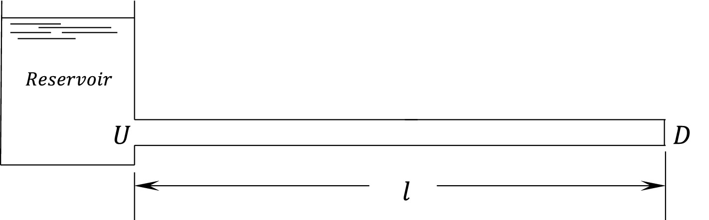
Figure 1. Reservoir-pipe system.

In which, $Z_c=\frac{a^2\mu }{\mathit{\text{igAω}}}$ is the characteristic impedance, $\mu =\frac{\mathit{i\omega }}{a}\sqrt{(1+\frac{f\mid Q_0\mid }{\mathit{\text{iωDA}}})}$ is the propagation constant, and the subscripts $D$ and $U$ denote the downstream and upstream ends of the pipe, respectively.

Frequency domain analysis can be performed using either the impedance or transfer matrix method. Both methods are based on the transient flow equations, but the transfer matrix often has benefits when analyzing topologically complex systems (Chaudhry, 2014; Streeter and Wylie, 1993). The transfer matrix method is incorporated here. Leakage is modeled here using Equation 7 (Ranginkaman et al., 2016):

$\begin{array}{ll}\sum _{i=1}^{{\mathit{ni}}_j}{q}_{\mathit{Di}}-\sum _{i=1}^{{\mathit{no}}_j}{q}_{\mathit{Ui}}-q_l=d_j& (7)\end{array}$

where, $q_l=\left(\frac{Q_{l0}}{2H_{l0}}{h}_l\right)$ is the linearized equation of the rate of flow from the leak (Lee et al., 2005), $h_l$ , $Q_{l0}$ and $H_{l0}$ are the local head fluctuations at the leak, the steady-state leakage discharge, and the steady-state head at the leak, respectively, where node $j$ is the leak location, ${\mathit{ni}}_j$ = the number of pipes entering node j, ${\mathit{no}}_j$ = the number of pipes exiting node j. $q_{\mathit{Ui}}$ = the exiting rate of the flow from node j by pipe i, $q_{\mathit{Di}}$ = the rate of flow entering node j by the pipe i, $d_j$ = the demand at node j, and the remaining parameters are defined as before. Taking the Fourier transform with respect to time gives the following frequency domain at the leakage location, we get Equation 8 (Ranginkaman et al., 2016):

$\begin{array}{ll}\sum _{i=1}^{{\mathit{ni}}_j}{\widehat{q}}_{\mathit{Di}}-\sum _{i=1}^{{\mathit{no}}_j}{\widehat{q}}_{\mathit{Ui}}-\frac{Q_{l0}}{2H_{l0}}{\widehat{h}}_j={\widehat{d}}_j& (8)\end{array}$

For the frequency-domain transient analysis of the pipe network in this study, we utilized a MATLAB-based computational package, which is based on the above formulation and the transfer matrix method.

2.2 Transient flow generation

The efficacy of ITA hinges on the generation of transient flow, which drives the inverse process by eliciting a measurable system response to a controlled excitation. This excitation serves as the foundation for both TITA and FITA methods, enabling the identification of leak parameters and pipe friction factors through the analysis of pressure or flow perturbations. For ITA to succeed, the characteristics of the transient excitation must satisfy several critical criteria: duration, amplitude, and location of the disturbance. Each of these factors significantly influences the quality and interpretability of the system response, directly impacting the accuracy and efficiency of leak detection and network calibration. Vítkovský et al. (2007) experimentally investigated the effects of valve closure time on the ITA’s accuracy. They concluded that the bandwidth of the transient flow, which is created by slow valve closure, is insufficient to carry the necessary information. Jung and Karney (2008) showed that using the mild transient with many measurement sites can increase the accuracy of the ITA. Haghighi and Shamloo (2011) designed the optimal excitation for generating transients in WSNs by presenting a mathematical programming method that optimizes the duration, amplitude, and location of excitation, considering the generated maximum and minimum pressure heads. Lee et al. (2014) suggested that, for practical fault detection, it is better to use both high and low-bandwidth signals.

The duration of the excitation determines the temporal window over which the transient signal evolves. Short, rapid excitations, such as those induced by a sudden valve closure, generate sharp pressure waves that propagate through the network, producing distinct reflections from leaks or other anomalies. All previous works advocated for such rapid excitations, citing examples like pump trips or the manual closure of a side-discharge valve, which create high-frequency transients capable of revealing system faults. However, excessively prolonged excitations may dampen these reflections, blur the signal, and reduce the resolution of TITA’s time-domain analysis or FITA’s FRD. Conversely, an overly brief disturbance may fail to excite lower-frequency modes, limiting the applicability of methods like the DFs approach, which relies on resonant peaks in the FRD.

The amplitude of the excitation governs the strength of the pressure wave and, consequently, the signal-to-noise ratio in the measured response. A sufficiently large amplitude ensures that leak-induced perturbations are distinguishable from background noise or minor hydraulic variations, enhancing the sensitivity of both TITA and FITA. However, practical constraints, such as avoiding damage to aging infrastructure or exceeding operational pressure limits, necessitate a balance between amplitude and safety.

The location of the disturbance is equally pivotal, as it dictates the propagation path of the transient wave and the nodes most affected by the response. Strategic placement near critical junctions or suspected leak sites can maximize the visibility of anomalies in the system’s response, whether analyzed in the time domain or frequency domain (Haghighi and Shamloo, 2011). For TITA, an excitation near the leak enhances the clarity of reflected pressure signals; for FITA and the DFs method, it amplifies shifts in the FRD’s dominant frequencies. However, not all excitation methods proposed by Lee et al. (2006) are universally ideal. For instance, while side-discharge valve closures offer precise control over timing and location, their effectiveness depends on network topology, loops or branches may diffuse the transient signal, reducing its diagnostic power.

Notably, the choice of excitation method must align with the analytical framework of ITA. TITA benefits from excitations that produce clear, time-resolved wave reflections, necessitating rapid and localized disturbances. FITA, and particularly the DFs method, thrives on excitations that excite a broad spectrum of frequencies, enabling the identification of resonant peaks sensitive to leaks. Valve maneuvers offer customizable duration and amplitude tailored to specific network conditions. Thus, the success of ITA, whether through TITA’s iterative optimization or FITA’s frequency-based efficiency, relies on designing an excitation that balances these criteria to elicit a robust and interpretable system response.

In practice, the design of an ideal excitation is naturally highly dependent upon the physical specifications of the system. Therefore, for leak detection in the field by the ITA, a wide variety of excitations should be investigated to achieve a transient flow, which could reflect the leak’s effects appropriately. Another issue that should be considered to generate a transient is that, to control the FDA linearization errors, the amplitude of excitation should be capped at 10% of the steady-state flow (Lee and Vitkovsky, 2010; Ranginkaman et al., 2019).

2.3 Measurement site design

The success of ITA, whether in the time domain (TITA) or frequency domain (FITA), relies heavily on the strategic deployment of pressure sensors within a WSN to capture transient signals for comparison with simulation outputs. This process estimates critical system parameters such as leak locations, sizes, and pipe friction factors. However, practical implementation is non-trivial due to challenges including limited site accessibility, sensor reliability, and network complexity. Unknown parameters, such as leaks, blockages, and friction factors affect pressure heads throughout the network, underscoring the need for measurement sites with heightened sensitivity to these variables. Selecting such locations enhances the ITA’s ability to discern the impacts of leaks and friction, improving diagnostic accuracy (Liggett and Chen, 1994; Zhang et al., 2019; Pan et al., 2022).

To optimize parameter estimation, the ITA objective function must leverage measurements from these sensitive sites, amplifying gradients within the optimization search space and enhancing problem convexity for reliable convergence. This necessitates robust methodologies to determine the optimal number and placement of sampling sites, specifically frequency responses for FITA, across a WSN’s numerous nodes.

Early efforts to address this challenge include Liggett and Chen (1994), who used sensitivity matrices to maximize information gain from pressure measurements, though their approach required significant computational resources. Vítkovský et al. (2003) presented a valuable approach for determining the configuration of measurement sites that produces optimal results for ITA. Three performance indicators based on A- and D-optimality criteria and the sensitivities of the heads concerning the unknown parameters were used in that study. They used a GA to find the optimal measurement locations according to the aforementioned criteria. Shamloo and Haghighi (2010) similarly used the sensitivities of transient heads to unknown leaks at candidate sites to rank the best locations for installing sensors for doing ITA.

More recent studies have built on this foundation. Zhang et al. (2019) proposed a sensor placement strategy using inverse transient analysis, optimizing locations based on sensitivity to pipeline conditions, albeit with reliance on optimization algorithms. Pan et al. (2022) advanced this field by introducing a sensitivity-based approach for transient-based leak detection, emphasizing computational efficiency and site diversification, though still requiring numerical optimization in some cases. Ayati and Haghighi, (2023) introduced a novel sampling design method for hybrid Machine Learning/Transient-Based (ML/TB) leak detection of pipe networks. Their proposed technique exploits the hydraulic responses of the network in the frequency domain and the concept of Filter and Wrapper feature selection. They also utilized multiobjective optimization to handle the trade-off between leak detection error and the number of sampling nodes. While these methods offer valuable insights, they often entail drawbacks such as high computational demands, the need for optimization, and potential numerical instabilities (e.g., ill-conditioned matrices), limiting their scalability in complex WSNs.

This study employs DTM (Ayati et al., 2019) to design optimal measurement sites, offering a computationally efficient and practical alternative. DTM prioritizes nodes based on their sensitivity rank to decision variables (e.g., leak parameters and friction factors) rather than absolute sensitivity values. This rank-based approach mitigates the influence of extreme sensitivities, fostering a more uniform distribution of sites, a critical advantage for detecting distributed or multiple leaks in looped networks. Unlike optimization-heavy methods, DTM requires no mathematical programming, Hessian matrix computation, or iterative algorithms, reducing computational overhead while maintaining diagnostic accuracy.

For FITA, DTM is adapted to focus on nodes with significant sensitivity to changes in FRD, leveraging the frequency domain’s inherent efficiency. The method evaluates sensitivity to leak parameters and friction factors independently and then integrates these rankings to produce a cohesive measurement site design that supports both leak detection and calibration. The DTM approach is implemented as follows:

1. The sensitivity of the nodes’ frequency responses to unknown parameters is calculated using Equations 7, 8. Each row of these matrices is ranked in terms of the sensitivity value and stored in matrices named $\text{Rank}\_a$ and $\text{Rank}\_f$ . So the element with the highest degree of sensitivity takes rank no. 1, and the element with the lowest sensitivity takes the rank $N_s$ (Equations 9, 10) (Ayati et al., 2019).

$\begin{array}{ll}S{a}_{\mathit{ij}}=\sum _{k=1}^M\mid \frac{\partial {\widehat{h}}_{\mathit{kj}}}{\partial {\mathit{Ae}}_i}\mid i=1\text{to}\mathit{NL}\text{and}j=1\text{to}\mathit{NS}& (9)\end{array}$

$\begin{array}{ll}S{f}_{\mathit{ij}}=\sum _{k=1}^M\mid \frac{\partial {\widehat{h}}_{\mathit{kj}}}{\partial f_i}\mid i=1\text{to}\mathit{NP}\text{and}j=1\text{to}\mathit{NS}& (10)\end{array}$

where $S{a}_{\mathit{ij}}$ is the pressure sensitivity matrix of site j concerning the leak area ${\mathit{Ae}}_j$ , $S{f}_{\mathit{ij}}$is the sensitivity matrix of the pipe friction factor $f_i$ in $\mathit{NS}$ (possible) candidate node as a location for pressure measurement, $\mathit{NL}$ is the number of leaks in the network, and $\mathit{NP}$ is the number of main pipes in the network.

2. The summation of rank in each node is stored in two vectors named $\mathrm{Sum}\_a$ (Equation 11) and $\mathrm{Sum}\_f,$ (Equation 12), which indicate the sum of ranks in each candidate node concerning the unknown parameters of the leak and the pipe friction factors, respectively.

$\begin{array}{ll}\mathrm{Sum}\_a_j=\sum _{i=1}^{\mathit{NL}}\text{Rank}\_a_{i,j}j=1\text{to}\mathit{NS}& (11)\end{array}$

$\begin{array}{ll}\mathrm{Sum}\_f_j=\sum _{i=1}^{\mathit{NP}}\text{Rank}\_f_{i,j}j=1\text{to}\mathit{NS}& (12)\end{array}$

3. In matrices of $\text{Rank}\_a$ and $\text{Rank}\_f$ , the node with the lowest value of rank summation is selected as the first measurement site. It means that this node has the highest priority in comparison with other nodes.

4. Rows that have the rank no. 1 for the selected node in step 3 are removed from $\text{Rank}\_a$ and $\text{Rank}\_f$ . As the selected node has the best priority for these unknowns (leaks and friction factors), the effect of these parameters is eliminated in future selections. It should be noted that in $\_a$ , each row indicates the effect of the leak at a node of the network, and in $\text{Rank}\_f$ each row indicates the effect of the loss coefficient in a pipe. In other words, the number of rows in $\text{Rank}\_a$ and $\text{Rank}\_f$ is equal to the number of nodes and pipes of the network, respectively.

5. If all rows of $\text{Rank}\_a$ and $\text{Rank}\_f$have been removed in step 4, the algorithm goes to step 6, and if not, the $\mathrm{Sum}\_a$ and $\mathrm{Sum}\_f$ are recalculated by the new values from step 4, and the algorithm returns to step 3.

6. Update $\mathrm{Sum}\_a$ and $\mathrm{Sum}\_f$ vectors. The new Rank matrix is taken into account for the new computations, and the algorithm returns to step 2.

7. In case all candidate nodes are selected, the algorithm is stopped. The nodes that are selected sooner have higher priority. It means that the selection of $N_s$ nodes out of the total NTS candidate nodes, it is enough that the first $N_s$ nodes are selected from DTM. Figure 2 shows the flowchart of this method, schematically.

Figure 2

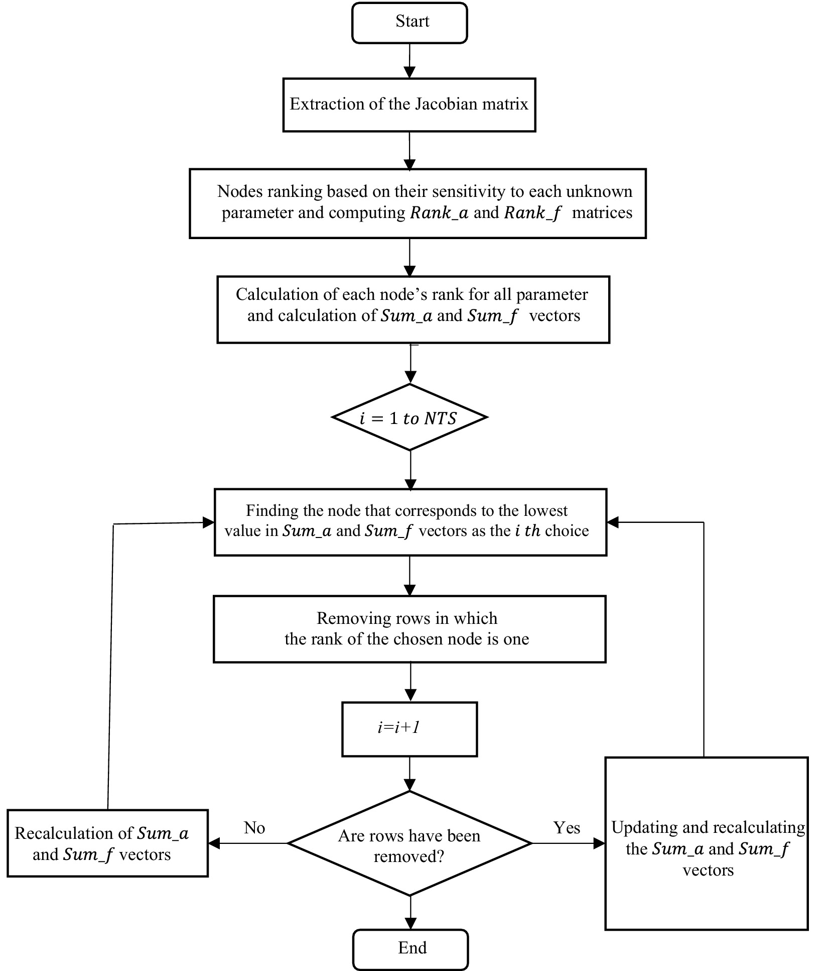
Figure 2. DTM flowchart.

2.4 Methodology of leak detection and calibration by FITA

Based on the transient excitation in the network and the transient pressure heads sampled at predetermined measurement sites, the ITA method can be applied. Since the TITA has been extensively developed and explained in previous studies (Liggett and Chen, 1994; Kapelan et al., 2003, 2004; Shamloo and Haghighi, 2009, 2010; Haghighi and Ramos, 2012), this section focuses exclusively on the step-by-step formulation of the FITA.

1. Excitation of transient flow: a transient event is introduced into the network by imposing a rapid change in a nodal demand or valve operation. This perturbation generates a propagating transient signal that interacts with system anomalies, such as leaks.

2. Data acquisition and frequency transformation: transient pressure heads are recorded at selected measurement sites with the highest possible sampling frequency to capture the full spectral characteristics of the transient response. The recorded time-domain pressure signals are then transformed into the frequency domain using the Fast Fourier Transform (FFT).

3. Development of the frequency-domain simulation model: a hydraulic simulation model of the water supply network is formulated in the frequency domain using the FDA. This model predicts the network’s frequency response as a function of both leak parameters and pipe friction factors. By representing the system behavior in the frequency domain, the effects of leaks manifest as distinct shifts in dominant frequencies, which can be utilized for leak localization and characterization.

4. Optimization formulation for leak detection: the inverse problem is formulated as a nonlinear programming (NLP) problem, where an objective function is defined to minimize the discrepancy between the measured and simulated frequency responses at the monitoring sites. The optimization is based on a least-squares criterion, ensuring that the estimated leak parameters minimize the overall error between observed and computed data. The objective function is expressed as shown in Equation 13 (Shamloo and Haghighi, 2010).

$\begin{array}{ll}C=\sqrt{\sum _{j=1}^{N_s}\sum _{i=1}^{\mathrm{N}}{({\widehat{h}}_{\mathit{Oij}}-{\widehat{h}}_{\mathit{mij}})}^2}& (13)\end{array}$

where, ${\widehat{h}}_{\mathit{mij}}$ and ${\widehat{h}}_{\mathit{Oij}}$ = the model predicted and observed frequency responses at site j for ith spectral data point, respectively, $N_s$ = the number of measurement sites in the network and the remaining parameters are as before. Objective function C is a function of all unknown parameters in the network, leaks and friction factors herein.

5. A nonlinear optimization solver is applied to solve the above problem. When the objective function is minimized to zero, the optimum decision variables represent the states of leakage and pipe friction factors in the network (Equation 13).

A similar approach is employed in the time domain using TITA. Following this method, the initial analysis identifies potential leakage-prone areas within the network. To enhance the accuracy of leak localization, a refined modeling approach can be adopted by incorporating sub-main pipelines into the primary network model.

In this refinement process, all relevant data about the sub-main branches, including physical attributes and hydraulic conditions, must be accurately gathered and integrated into the model. If necessary, additional monitoring nodes can be strategically placed within the sub-main network to improve the resolution of the analysis. The leak detection procedure is then repeated using these expanded datasets, ensuring a more precise and reliable localization of leaks.

By iteratively refining the network representation and optimizing measurement site selection, both TITA and FITA can be effectively adapted for real-world applications, where network complexity and uncertainty pose significant challenges to accurate leak detection.

3 Case study

The FITA and TITA methods are applied to a benchmark WSN originally introduced by Pudar and Liggett (1992) for leak detection and calibration, which has since been widely used as a case study in numerous investigations. The plan and physical properties of the network are shown in Figure 3. A small leak with an effective area of $A_e=1c{m}^2$ is located at Node 2, and the transient flow is induced by a sudden change in demand at Node 4 (Figure 4). This example aims to examine the impact of leakage on the network’s frequency response and to compare the results of the FITA and TITA methods.

Figure 3

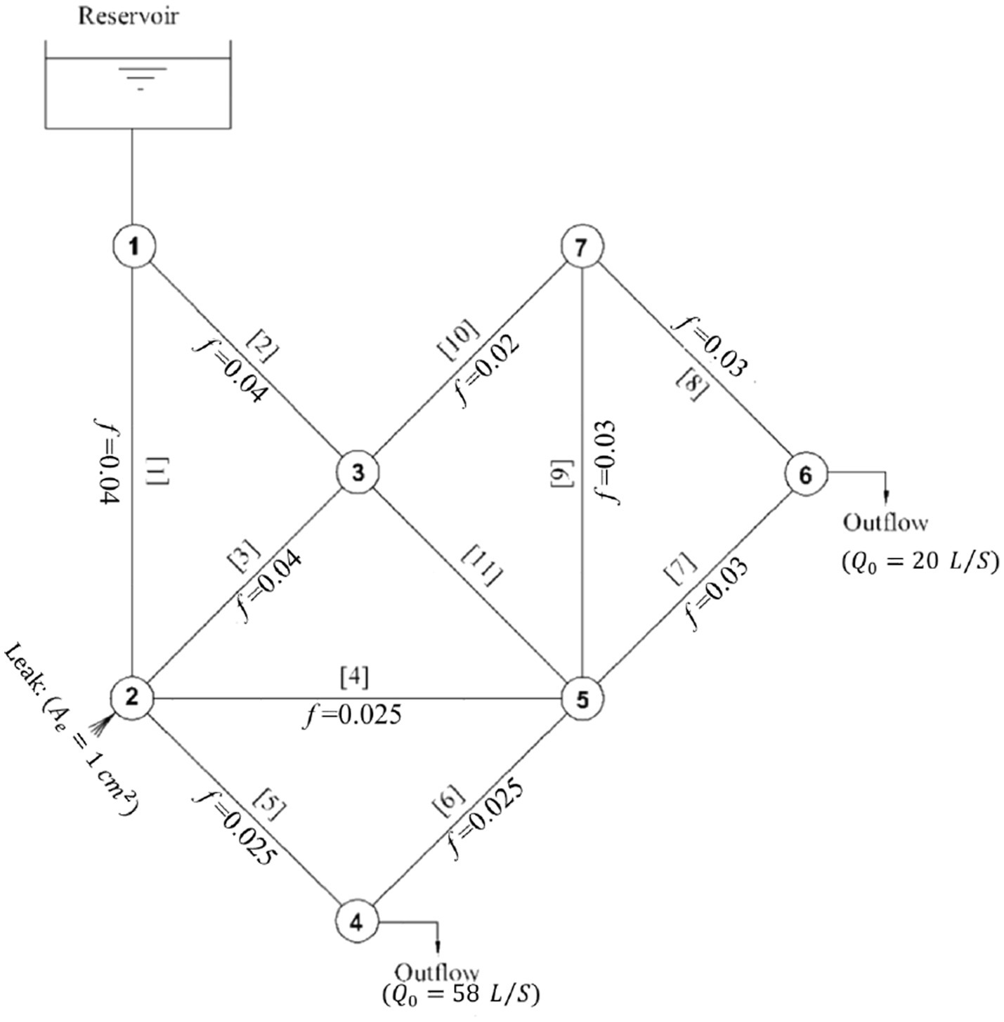
Figure 3. Test case water supply network.

Figure 4

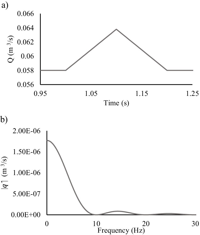
Figure 4. The excitation at nodes 4, (a) in the time domain and (b) in the frequency domain.

3.1 Designing the optimum measurement sites

In the first step, DTM and the methods proposed by Vítkovský et al. (2003) are employed to determine the optimal measurement sites. Vítkovský et al. (2003) introduced three key indicators for evaluating the optimal performance of the ITA for a given configuration of measurement sites: ${\eta }_J$ , which is based on the Jacobian of the heads and should be maximized; ${\eta }_A$ , which follows the A-optimality criterion and should be minimized, as it represents the variance of parameter errors; and ${\eta }_D$ , which follows the D-optimality criterion and should be maximized, as it accounts for the curvature and covariance matrices. For further details, refer to the original study (see Table 1).

Table 1

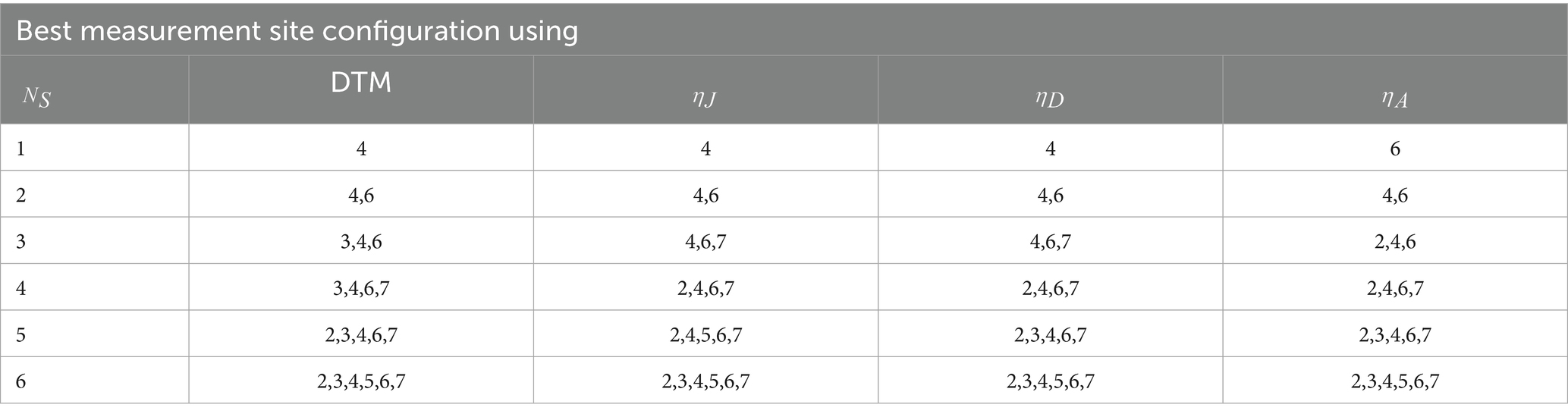
Table 1. Comparison of the results of DTM with Vítkovský et al. (2003) for leak detection.

As shown in Tables 2, 3, the results of DTM closely align with those obtained by Vítkovský et al. (2003). However, DTM offers a more straightforward and computationally efficient approach, as it does not require an optimization process. Based on the results, if only a single measurement site is to be selected, Node 4 is identified as the optimal location for sensor installation. However, when considering the installation of two sensors, Nodes 4 and 6 are preferred, as they provide more comprehensive coverage of the network’s frequency responses and offer better sensitivity for detecting anomalies such as leaks.

Table 2

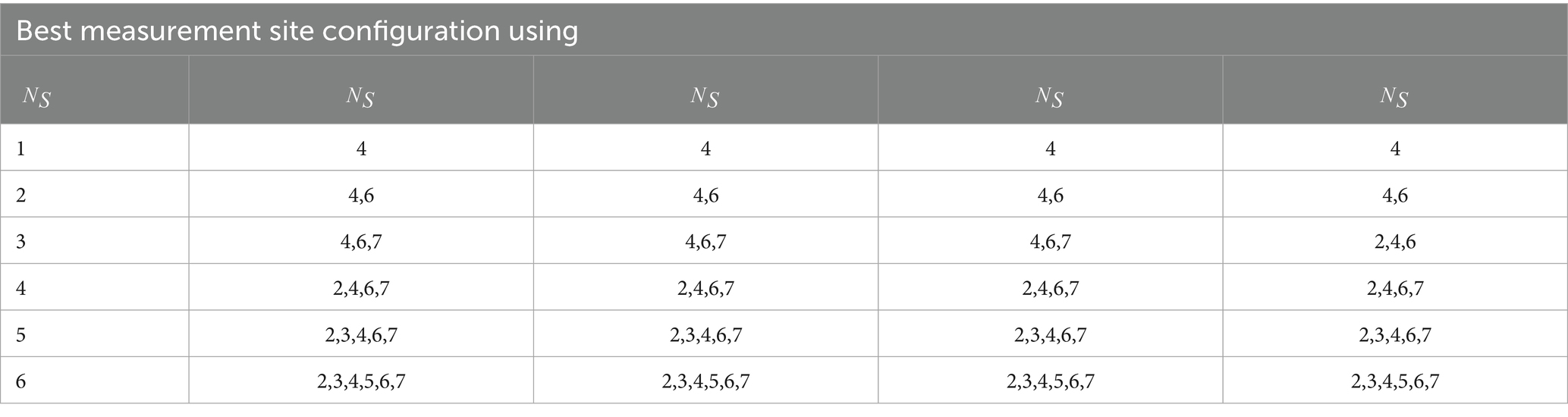
Table 2. Comparison of the results of DTM with Vítkovský et al. (2003) for calibration of friction factors.

Table 3

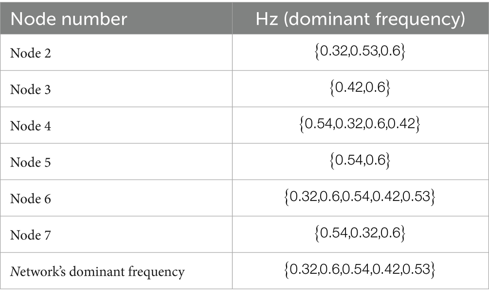
Table 3. Dominant frequencies.

3.2 Concept of dominant frequencies

Before addressing leak detection and calibration of friction factors using the FITA and TITA methods, a general analysis of the network’s frequency response is conducted for both leaking and non-leaking scenarios. The frequency response function (FRF) diagrams of the network, obtained from excitation at Node 4 for the non-leaking case, are presented in Figure 5. The FRF describes how a system reacts to different input frequencies, providing insights into its dynamic behavior. In pipeline networks, the FRF represents the relationship between pressure fluctuations and flow disturbances, allowing for a detailed analysis of system responses under various conditions. This method is beneficial for leak detection, as differences in frequency responses between leaking and non-leaking scenarios can reveal anomalies.

Figure 5

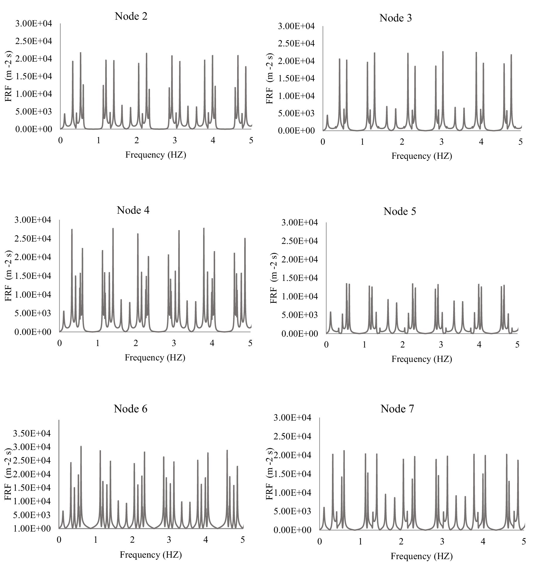
Figure 5. The FRF diagrams of the network for the non-leaking case.

The FRF is computed by analyzing how the pressure head reacts to an applied excitation. After the transient event was initiated in the network and the frequency responses of the network at nodes were computed, the FFT was applied to the excitation (Figure 4a) converting it into the frequency domain (Figure 4b). The nodal FRF is obtained by dividing the frequency responses of nodal heads by the FFT of the excitation, revealing how different frequency components propagate through the network. This method helps in leak detection and system analysis by identifying frequency-dependent behavior.

Figure 5 shows that the FRF diagram values are repeated at the same frequency intervals. As seen, the frequency range of the first harmonic is ( $0\le \omega \le 1.75$ ), the second harmonic is ( $1.75\le \omega \le 2\ast 1.75$ ) and so on up to the end. Regarding the similarity of the shape of all the FRF harmonics, only the first harmonic could be taken into account. Each harmonic of the FRF consists of two identical parts that have axial symmetry. Therefore, the second part of the first harmonic could be removed, and only the first part could be considered (Figure 6).

Figure 6

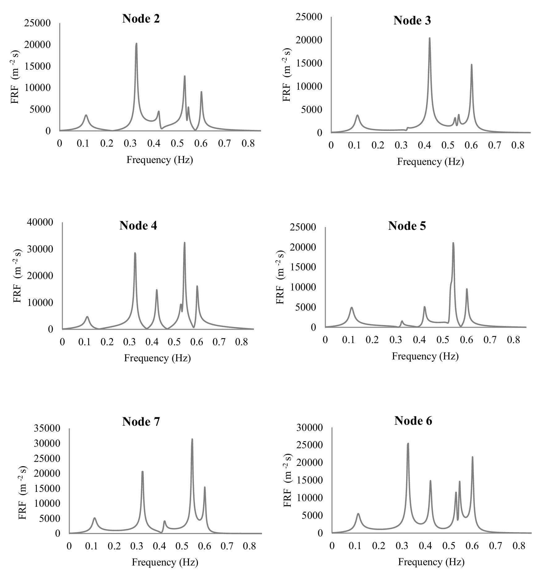
Figure 6. The first half of the first harmonic of the FRF diagrams for the non-leaking case.

Figure 5 illustrates the FRF diagram, where the response values repeat at regular frequency intervals, indicating a periodic structure. As observed, the frequency range of the first harmonic extends from 0 to 1.75 (i.e., $0\le \omega \le 1.75$ ), while the second harmonic spans 1.75 to 2 × 1.752, and this pattern continues across higher harmonics. Due to the self-similar nature of the FRF across different harmonic ranges, the analysis can be simplified by focusing solely on the first harmonic, as it captures the essential characteristics of the system’s frequency response. Furthermore, each harmonic in the FRF exhibits axial symmetry, meaning it consists of two mirrored sections. This symmetry arises due to the properties of the Fourier transform in linear time-invariant systems, where the frequency response in the positive spectrum mirrors the negative spectrum. Consequently, the second half of the first harmonic contains redundant information and can be disregarded without loss of accuracy. As a result, only the first half of the first harmonic is retained for further analysis, as depicted in Figure 6, leading to a more efficient representation of the system’s frequency behavior.

The FRF diagrams exhibit peak values that vary depending on the location of the node within the network. In this study, the DFs are defined as the frequencies corresponding to peak values in the FRF diagram that exceed half of the maximum peak value. These DFs represent the most significant resonant responses of the system. Since each node may exhibit different DFs due to variations in local hydraulic conditions and wave reflections, the set of all DFs across the network collectively defines the network’s DFs. The DFs identified for each node in the studied network are summarized in Table 3, providing insights into the system’s dynamic behavior and potential resonance characteristics.

When a leak occurs at a node, the most significant changes in the FRF diagram are expected to appear at the DFs of that node. This is because the DFs represent the natural resonance points of the system, where pressure and flow perturbations are most sensitive to disturbances such as leaks. The presence of a leak alters the hydraulic impedance of the network, modifying the frequency response by shifting peak amplitudes or introducing new frequency components. Figure 7 illustrates the FRF diagram of Node 6 (as a measurement site) under both non-leaking and leaking conditions for different leak locations. The comparison of these diagrams highlights how leaks influence the network’s frequency response, providing a basis for detecting and localizing leaks based on deviations at the dominant frequencies.

Figure 7

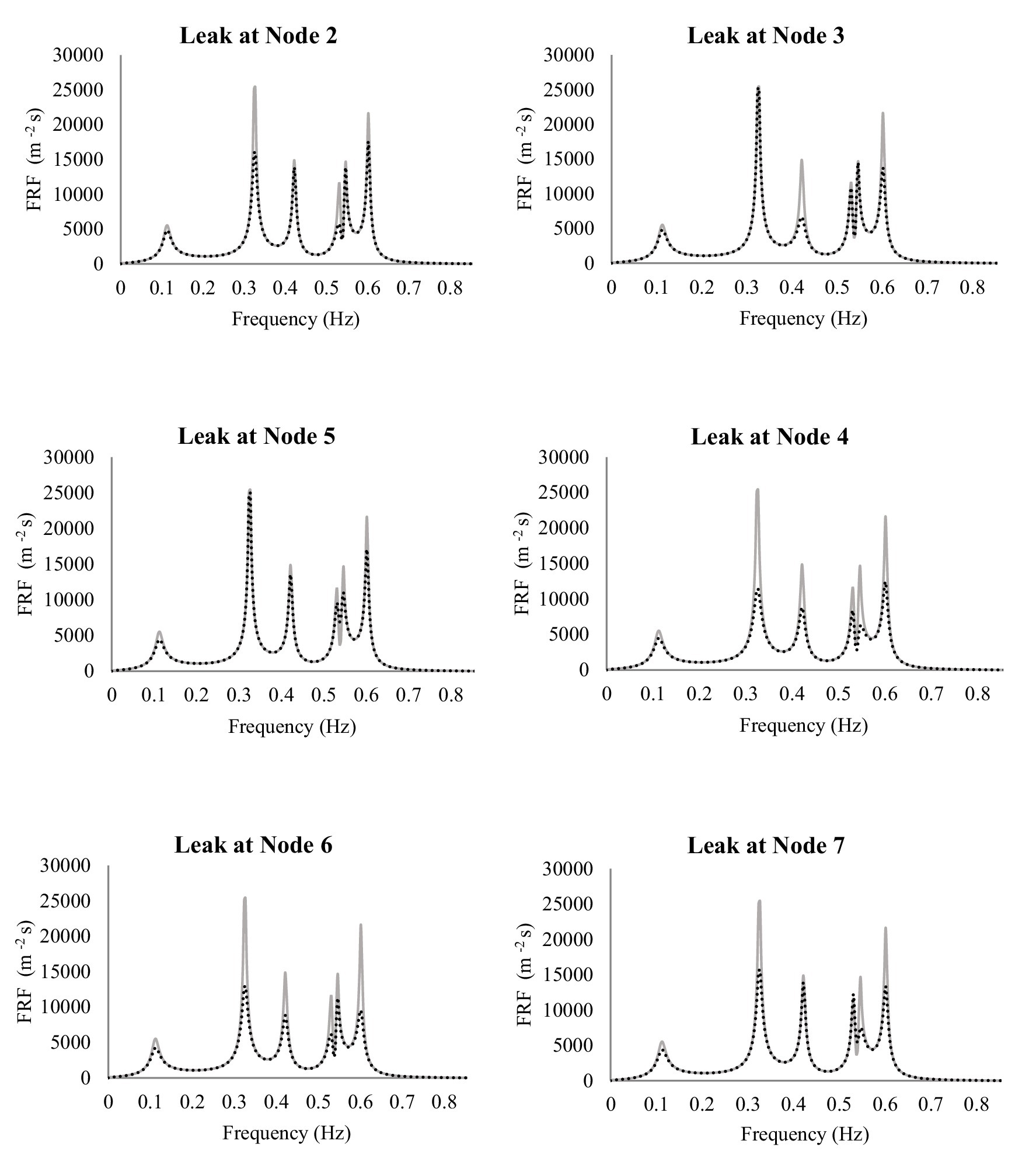
Figure 7. The FRF diagram of node 6 for non-leaking and leaking cases for different leak locations.

By comparing Figure 7 with Table 3, it becomes clear that the concept of DFs can be effectively utilized for both leak detection and sensor placement design. The leak detection process using the DFs method is as follows:

• Step 1: The DFs for each node are determined based on the FRF diagram under non-leaking conditions. These frequencies serve as baseline markers for identifying potential leaks.

• Step 2: The measured FRF diagrams at the selected measurement sites are compared with the non-leaking FRF diagram obtained in Step 1. If the measured FRF diagrams match the non-leaking baseline, it indicates no leakage. However, if there are discrepancies, the frequencies corresponding to the most significant variations in the FRF diagram values are identified, which highlights the potential areas of disturbance caused by leaks.

• Step 3: The frequencies identified in Step 2 are then compared to the DFs table (Table 3). If any of the identified frequencies match the DFs of a particular node, it indicates that a leak is present at that node. This method enables accurate leak localization based on variations in frequency responses at critical locations within the network.

The following questions may arise: Does the generated pattern in the FRF diagram remain preserved as the effective leak area increases? And can this method be applied to leaks with a larger area? The answer to both of these questions is yes. As the effective leak area increases, the variations in the FRF values at the DFs become more pronounced. This leads to more significant deviations in the FRF diagram, making the detection of the leak location easier. Figure 8 illustrates the FRF diagram at Node 6 for cases where the effective leak area at Node 2 varies between $\mathit{Ae}=1{\mathrm{cm}}^2$ and $\mathit{Ae}=4{\mathrm{cm}}^2$ . As the leak area increases, the changes in the FRF diagram are amplified, allowing for more accurate detection of the leak location and its severity. This demonstrates that the DFs method remains effective and even improves in its sensitivity to leak detection as the leak area expands.

Figure 8

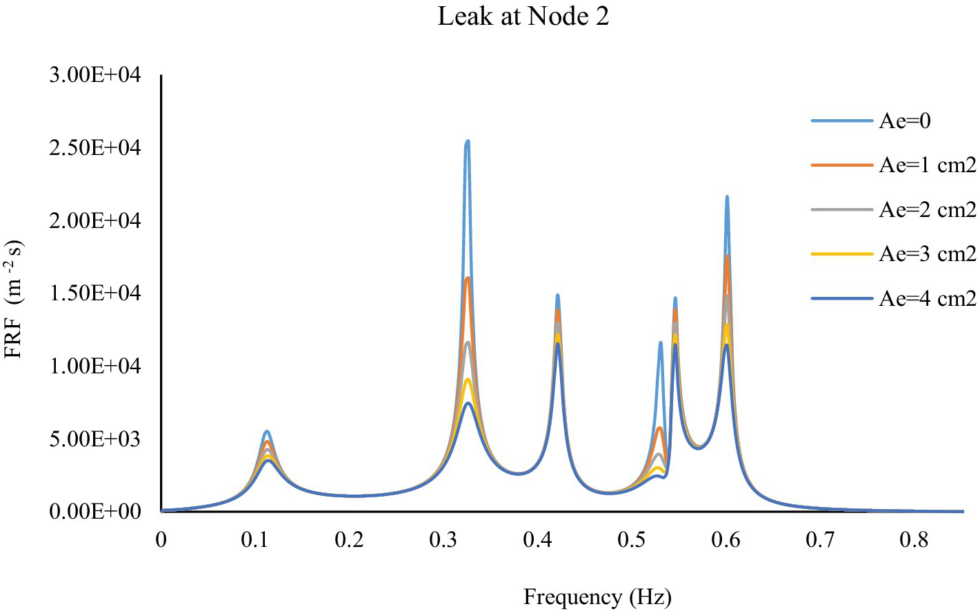
Figure 8. The impact of node 2’s leakage effective area on the FRF diagram at node 6.

According to the DFs concept, the optimal nodes for measurement sites are those whose DFs match the network’s DFs or have the highest number of matching frequencies. Based on the results presented in Table 3, Nodes 4 and 6 are identified as the best locations for sensor installation, which aligns with the findings obtained through DTM in the previous section. However, it is important to note that the DFs method is not universally applicable to all WSNs. Its effectiveness is highly dependent on factors such as the resolution of transient flow data and the shape and scale of the network. Despite these limitations, the DFs method shows potential as a supplementary tool for leak detection and measurement site design, complementing existing approaches. Further investigations are necessary to fully assess its applicability and refine the method for broader use across different network configurations.

3.3 Leak detection by FITA and TITA

To solve the problem using the ITA approach, due to the unknown location and number of leaks, all junction nodes except the reservoir are assumed to be potential leaky nodes with unknown sizes. Consequently, the problem consists of 17 unknown decision variables: 6 of these correspond to the leak’s effective areas ( $\mathit{Ae}$ ) of the leaky nodes, while the remaining 11 parameters represent the pipe friction factors ( $f$ ) for each pipe segment. To determine the unknown parameters, the objective function (Equation 13) at Node 4 (as the only selected measurement site) is minimized to zero using a real GA with the constraints $0\le \mathrm{Ae}\le 2{\mathrm{cm}}^2$ and $0.015\le f\le 0.05$ .

In our study, the GA parameters such as mutation rate, number of generations, population size, and crossover methods were determined using a well-established, statistically guided trial-and-error approach with a limited number of iterations. Accordingly, the optimization process began by generating an initial population of 100 chromosomes. The optimization was carried out with a uniform gene exchange mechanism, and the mutation rate decreased linearly from 0.03 in the first generation to 0.005 in the final generation. Tables 4, 5 summarize the responses obtained from the GA for the leakage effective area and the friction factor. After 70 and 140 generations, the objective function values were minimized to $9.523\times {10}^{-4}$ for FITA and $7.851\times {10}^{-4}$ for TITA, respectively, showing that both methods were able to converge to a solution with minimal error.

Table 4

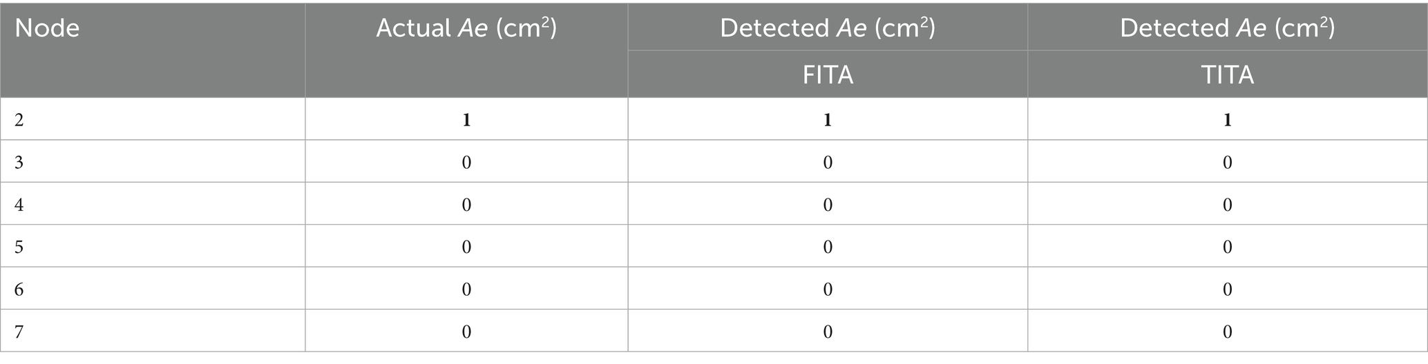
Table 4. Leak detection results of the FITA and TITA methods.

Table 5

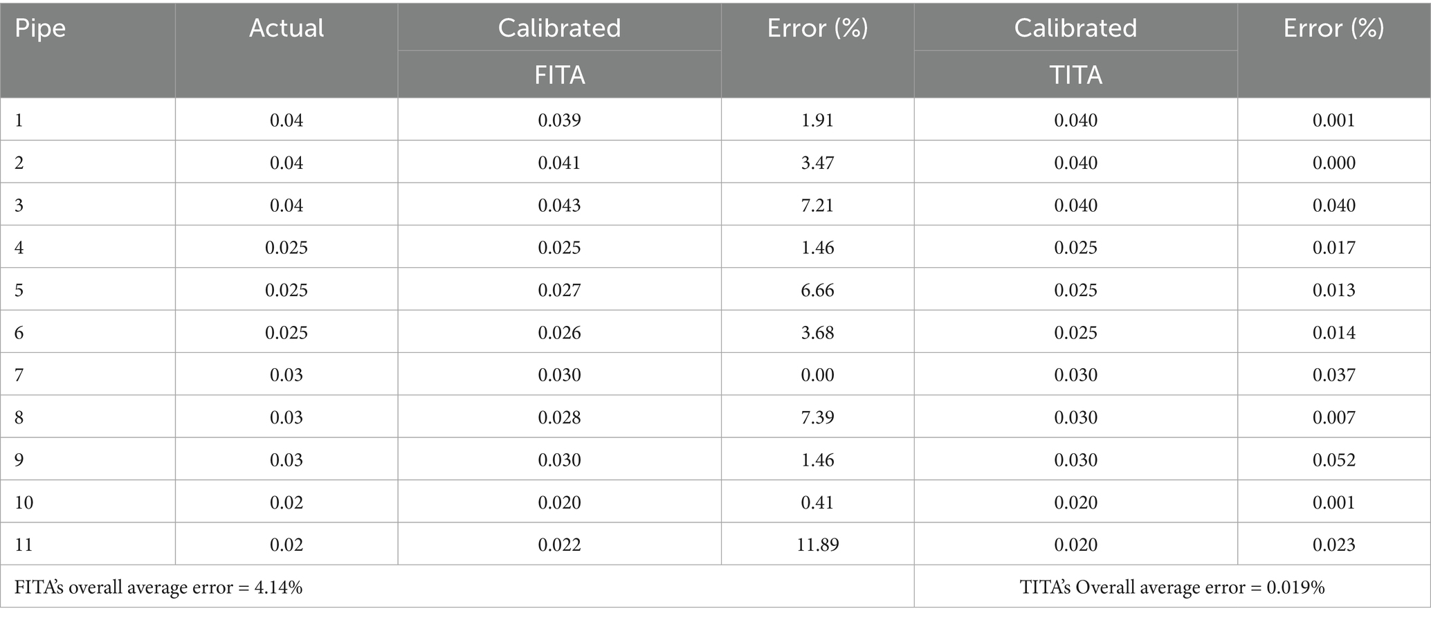
Table 5. Calibration results of the FITA and TITA methods.

Tables 4, 5 demonstrate that both FITA and TITA can accurately determine the effective area and location of leaks. However, the calibration results for friction factors from FITA are less accurate compared to TITA. This discrepancy can be attributed to the higher sensitivity of the frequency response to leak parameters, as opposed to the friction factors, as well as the linearization of the friction loss equation in FITA. The linearization in FITA may introduce approximations that reduce the accuracy, especially when compared to the more comprehensive approach in TITA, which directly accounts for the nonlinear behavior of friction loss. This combination of factors contributes to the relatively lower accuracy of FITA in determining the leak parameters. This represents one of the key advantages of using the frequency domain analysis for leak detection via the inverse method. Unlike TITA, where the accuracy of leak parameter determination heavily relies on the precise estimation of friction factors, the FITA method is more robust. It can yield acceptable results even when the friction factors vary within a reasonable range around their initial estimates. This suggests that, for leak detection with FITA, simultaneous calibration of friction factors is not essential; an initial estimate of the friction factors is sufficient. The following section will explore the impact of friction factor estimation on the accuracy of leak detection to further support this point.

3.4 Uncertainty in friction factors

To evaluate the impact of friction factor estimation uncertainty on the accuracy of leak detection, five distinct scenarios were considered. In the first and second scenarios, the friction factors for all pipes were assumed to be at their minimum and maximum values, namely, $f=0.015$ and $f=0.05$ , respectively. In scenarios three through five, the friction factors were randomly assigned within the range of the above values for each pipe. Table 6 presents the friction factor values for each scenario, alongside the percentage differences relative to the actual friction factor values used in the simulation. These scenarios help investigate how variations in friction factor estimates affect the performance and accuracy of leak detection methods, specifically FITA and TITA.

Table 6

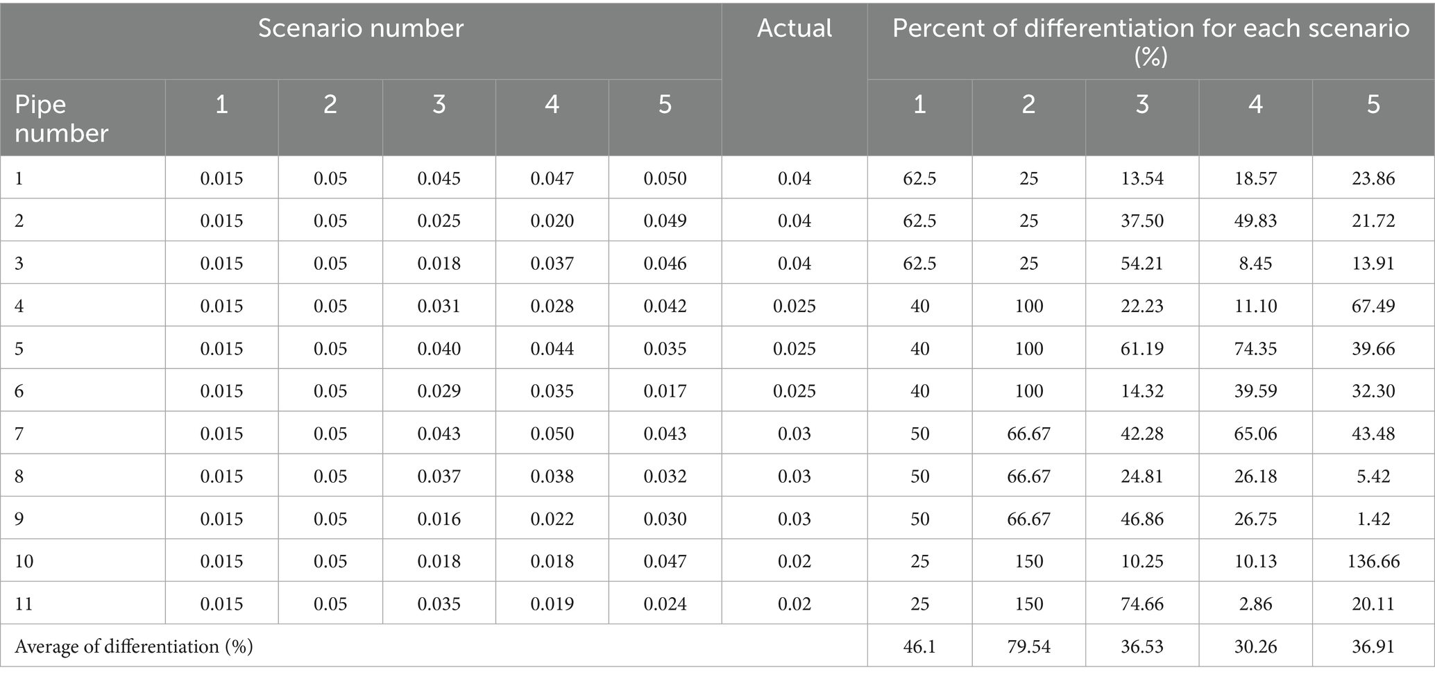
Table 6. Pipe friction factors scenarios.

In the next stage, leak detection was performed for each scenario using both FITA and TITA methods. Table 7 presents the mean errors of the estimated leak parameters for all scenarios, providing a comparison of the accuracy of leak detection under varying uncertainties in the friction factor values. These results allow for an evaluation of how different assumptions about the friction factors impact the performance of the leak detection process using both methods.

Table 7

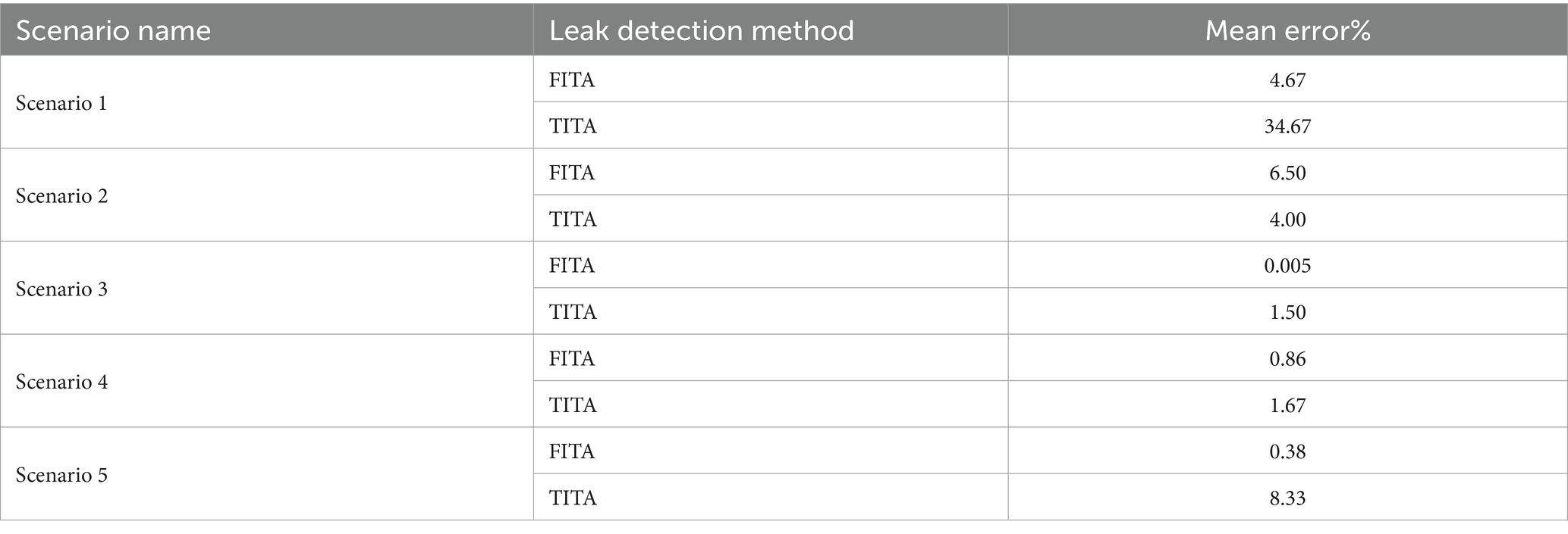
Table 7. Mean error of the estimated leak parameters for the pipe friction scenarios.

As shown in Table 7, the FITA method is more sensitive to leakage than to the pipe friction factors. This sensitivity allows for acceptable leak detection results without the need to perform calibration simultaneously with the leak detection process. Thus, an initial estimation of the friction factors is sufficient for the FITA method to provide reliable leak detection results.

In these scenarios, incorrect parameter values were intentionally introduced into the TITA and FITA models to assess the impact on leak detection accuracy. The scenarios are as follows: (1) A 10% error in the length of pipe 3, changing from 762 m to 838.2 m; (2) A 10% error in the wave speed of pipe 3, changing from 1,316 m/s to 1447.6 m/s; (3) A 10% error in the lengths of pipes 1 and 3, with changes from 762 m to 685.2 m and 762 m to 838.2 m, respectively, along with a 10% error in the wave speeds of pipes 2 and 4, changing from 1,316 m/s to 1447.6 m/s and 1,316 m/s to 1195.5 m/s, respectively. Table 8 presents the overall mean error and the maximum error in leak detection for each of the aforementioned scenarios.

Table 8

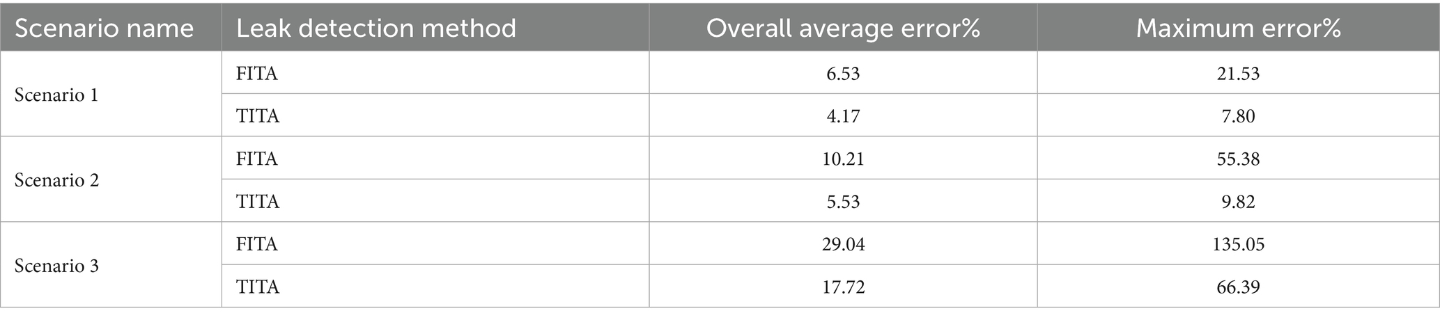
Table 8. Overall mean error and the maximum error of leak detection by TITA and FITA for uncertainty scenarios of friction factors.

Table 8 demonstrates that the FITA method exhibits greater sensitivity to variations in pipe length and wave speed compared to TITA. Consequently, uncertainties in the lengths of pipes and wave speeds can significantly impact the accuracy of the FITA method. Figure 9 illustrates the frequency response at node 4 under the uncertainty scenarios, contrasting these results with the actual conditions.

Figure 9

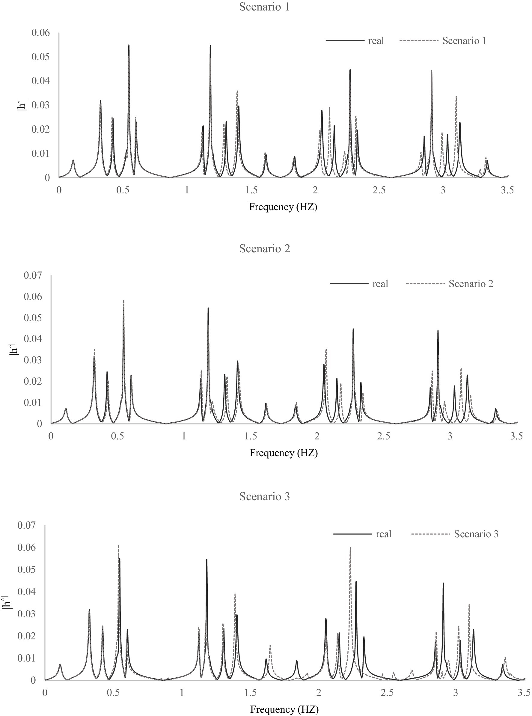
Figure 9. Frequency response at node 4 under different uncertainty scenarios of friction factors, illustrating the impact of friction variability on system dynamics.

We observe that uncertainties, particularly in pipe length and wave speed, induce shifts in the DFs of the system by altering transient signal travel times, as demonstrated in Figure 9. These shifts lead to discrepancies between predicted and actual system behaviors, resulting in less accurate leak detection and an increased likelihood of false alarms, especially in complex and large-scale water supply networks. Notably, while FITA exhibits a high sensitivity to leak parameters, it is comparatively more sensitive to uncertainties in pipe length and wave speed than TITA. This is primarily because FITA relies on linearized frequency-domain models, which can be affected by nonlinearities and parameter variability. On the other hand, TITA, operating in the time domain, better accounts for nonlinear friction losses but may require friction factor calibration for improved accuracy.

Our results (Tables 7, 8) reveal that FITA can provide reliable leak detection without necessitating simultaneous calibration of friction factors, using just initial estimates. However, the accuracy of FITA deteriorates with increasing parameter uncertainties, highlighting the importance of precisely characterizing these uncertainties in practical applications. As such, effective practical implementation of ITA methods demands comprehensive uncertainty quantification and sensitivity analyses to accommodate parameter variability. In this context, our findings suggest that practitioners employing transient-based leak detection should prioritize precise measurements or estimations of pipe geometries and wave speeds to mitigate the adverse impacts of uncertainties. Future research should focus on developing advanced uncertainty modeling and robust calibration techniques that improve the resilience of FITA and TITA in operational environments. By explicitly acknowledging and addressing these uncertainties, our work guides practitioners in applying inverse transient analysis more effectively, thereby enhancing leak detection accuracy and operational reliability in real-world water supply networks.

In practical terms, as pipeline networks grow in scale and complexity, these types of uncertainties, including variations in pipe length, material properties influencing wave speed, and modeling assumptions, become more significant. Such uncertainties elevate the risk of false alarms in leak detection or condition assessment applications, reducing the robustness of transient-based diagnostic methods.

We observe that uncertainties, particularly in pipe length and wave speed, induce shifts in the dominant frequencies (DFs) of the system by altering transient signal travel times, as demonstrated in Figure 9. These shifts lead to discrepancies between predicted and actual system behaviors, resulting in less accurate leak detection and an increased likelihood of false alarms, especially in complex and large-scale water supply networks. Notably, while FITA exhibits a high sensitivity to leak parameters, it is comparatively more sensitive to uncertainties in pipe length and wave speed than TITA. This is primarily because FITA relies on linearized frequency-domain models, which can be affected by nonlinearities and parameter variability. On the other hand, TITA, operating in the time domain, better accounts for nonlinear friction losses but may require friction factor calibration for improved accuracy.

Therefore, for the effective deployment of ITA in real-world scenarios, it is essential to deepen the understanding of these uncertainties and their impacts on transient signal characteristics. This entails developing advanced modeling approaches, sensitivity analyses, and uncertainty quantification techniques that can better capture the influence of pipe length, wave speed variability, and other factors on system dynamics. Enhancing the reliability of FITA and ITA methods through such efforts will improve confidence in transient-based monitoring solutions applied to complex pipeline infrastructures.

For a more comprehensive understanding of the uncertainties associated with the transient simulation model and the ITA, readers can refer to studies such as Vítkovský et al. (2007), Jung and Karney (2008), Haghighi et al. (2012), and Sabzkouhi and Haghighi (2018). To obtain reliable results in real-world applications using ITA, it is essential to account for all the aforementioned challenges. Given the range of uncertainties inherent in the problem, ITA may, in some cases, yield inaccurate or false results.

4 Discussion and conclusion

This study conducted a comparative investigation of ITA methods for leak detection in WSNs, focusing on FITA and TITA approaches. The research demonstrated that both methods achieved equivalent leak detection accuracy (100% correct identification of leak location and size) but exhibited distinct performance characteristics. FITA provided superior computational efficiency, converging twice as fast, while maintaining acceptable accuracy without simultaneous friction factor calibration. TITA delivered higher friction factor calibration precision (0.019% versus 4.14% average error) but required greater computational resources. The novel DFs method enabled direct leak detection through frequency response analysis, while DTM proved effective for optimal sensor placement with reduced computational overhead. Uncertainty analysis confirmed FITA’s robustness to friction factor variations, establishing its suitability for large or complex networks with incomplete parameter knowledge.

The comparative analysis revealed fundamental trade-offs between FITA and TITA that have significant implications for practical leak detection. FITA’s computational advantage stemmed from its elimination of spatial discretization across the entire network, solving equations only at critical nodes and potential leak sites, which reduced the number of unknown parameters and simplified the optimization process. In contrast, TITA’s superior calibration accuracy reflected its comprehensive treatment of nonlinear friction behavior, making it more suitable for scenarios requiring precise parameter estimation. However, TITA’s higher sensitivity to friction factors necessitated simultaneous calibration, increasing computational demands, a limitation. The DFs method advanced beyond traditional FDA by exploiting natural resonance points for direct, analytical leak detection without iterative optimization. The DFs approach reduced detection time and improved sensitivity to leaks, as evidenced by the case study where DFs captured significant frequency response shifts at leak nodes. Similarly, DTM provided a rank-based approach to sensor placement that mitigated extreme sensitivities and promoted uniform site distribution, outperforming genetic algorithm-based methods in computational simplicity while maintaining accuracy for looped networks.

Uncertainty analysis highlighted differential impacts on FITA and TITA, guiding their practical application. FITA exhibited greater sensitivity to variations in pipe length and wave speed, causing shifts in dominant frequencies that could lead to false positives in complex networks. In contrast, TITA showed more robustness, but its performance degraded under friction factor uncertainties. These findings underscore that uncertainties in geometric and hydraulic parameters can distort transient signals, reducing detection reliability. For practical implementation, such uncertainties necessitate careful model validation; however, FITA’s ability to function with initial friction factor estimates makes it more forgiving in data-scarce environments.

Based on these insights, we offer the following evidence-based guidelines for practitioners:

1. Method Selection: Choose FITA for large-scale or complex WSNs, prioritizing computational efficiency and minimal calibration as it reduces unknown parameters and converges faster.

2. Uncertainty Management: Incorporate sensitivity analyses for pipe length and wave speed in FITA applications to mitigate frequency shifts; for TITA, prioritize accurate friction factor inputs. Use uncertainty quantification techniques to reduce false alarms, especially in aging infrastructure.

3. Sensor and Excitation Design: Leverage DFs for strategic sensor placement via DTM, minimizing the number of sites and excitation types that excite broad frequency spectra. This reduces costs while enhancing signal quality, addressing challenges like noise and suboptimal placement.

4. Network-Specific Considerations: For scaled-up applications, account for factors like network complexity, measurement noise, and signal resolution; hybrid FITA-TITA approaches may optimize trade-offs.

Future research should integrate FITA with advanced machine learning frameworks to leverage DFs as input features for automated leak pattern recognition across diverse network topologies. Researchers should extend the DFs method with deep learning models for adaptive frequency analysis under varying operating conditions. Implementation studies should evaluate hybrid FITA-TITA systems, using FITA for rapid initial screening and TITA for refined calibration. DTM should be enhanced for dynamic, adaptive sensor placement that responds to seasonal or demand-driven changes. Finally, comprehensive field validations are essential to test these methods in real-world settings, incorporating effects like measurement noise and hydraulic variability systems to advance operational reliability and water conservation.

Data availability statement

The raw data supporting the conclusions of this article will be made available by the authors, without undue reservation.

Author contributions

HR: Formal analysis, Writing – original draft, Writing – review & editing, Data curation, Visualization, Methodology. AB: Investigation, Validation, Writing – review & editing, Visualization, Funding acquisition, Writing – original draft. AH: Conceptualization, Writing – original draft, Software, Methodology, Investigation, Supervision, Data curation, Writing – review & editing, Formal analysis. SK: Writing – review & editing, Writing – original draft, Funding acquisition, Resources, Project administration. UD: Funding acquisition, Writing – original draft, Project administration, Writing – review & editing, Resources.

Funding

The author(s) declare that financial support was received for the research and/or publication of this article. We gratefully acknowledge the financial support provided by the Deutsche Forschungsgemeinschaft (DFG) for this project under project number 544048327.

Conflict of interest

The authors declare that the research was conducted in the absence of any commercial or financial relationships that could be construed as a potential conflict of interest.

Generative AI statement

The author(s) declare that no Gen AI was used in the creation of this manuscript.

Any alternative text (alt text) provided alongside figures in this article has been generated by Frontiers with the support of artificial intelligence and reasonable efforts have been made to ensure accuracy, including review by the authors wherever possible. If you identify any issues, please contact us.

Publisher’s note

All claims expressed in this article are solely those of the authors and do not necessarily represent those of their affiliated organizations, or those of the publisher, the editors and the reviewers. Any product that may be evaluated in this article, or claim that may be made by its manufacturer, is not guaranteed or endorsed by the publisher.

References

Abdelmoez, M. N., Ibrahim, K., Ali, A. S., and Heshmat, M. (2024). A standalone sensing and actuation IoT solution for water management, leakage detection, and localization problems. Water Conserv. Sci. Eng. 9:16. doi: 10.1007/s41101-024-00248-w

Crossref Full Text | Google Scholar

Ali, A. S., Abdelmoez, M. N., Heshmat, M., and Ibrahim, K. (2022). A solution for water management and leakage detection problems using IoTs based approach. Int. Things 18:100504. doi: 10.1016/j.iot.2022.100504

Crossref Full Text | Google Scholar

Ayati, A. H., Ranginkaman, M. H., Bakhshipour, A. E., and Haghighi, A. (2019). Transient measurement site design in pipe networks using the Decision Table Method (DTM). J. Hydraul. Struct. 5, 32–48. doi: 10.22055/jhs.2019.29402.1107

Crossref Full Text | Google Scholar

Ayati, A. H., and Haghighi, A. (2023). Multiobjective wrapper sampling design for leak detection of pipe networks based on machine learning and transient methods. J. Water Resour. Plann. Manage. 149, 02023001. doi: 10.1061/JWRMD5.WRENG-5620

Crossref Full Text | Google Scholar

Capponi, C., Ferrante, M., Zecchin, A. C., and Simpson, A. R. (2017a). Leak detection in a branched system by inverse transient analysis with the admittance matrix method. Water Resour. Manage. 31, 4075–4089. doi: 10.1007/s11269-017-1730-6

Crossref Full Text | Google Scholar

Capponi, C., Zecchin, A. C., Ferrante, M., and Gong, J. (2017b). Numerical study on accuracy of frequency-domain modelling of transients. J. Hydraul. Res. 55, 813–828. doi: 10.1080/00221686.2017.1335654

Crossref Full Text | Google Scholar

Chaudhry, M. H. (2014). Applied hydraulic transients, vol. 415. New York: Springer, 31–42.

Google Scholar

Colombo, A. F., and Karney, B. W. (2002). Energy and costs of leaky pipes: toward comprehensive picture. J. Water Resour. Plan. Manag. 128, 441–450. doi: 10.1061/(ASCE)0733-9496(2002)128:6(441)

Crossref Full Text | Google Scholar

Covas, D., and Ramos, H. (1999). “Leakage detection in single pipelines using pressure wave behavior.” Proc., Water Industry Systems: Modeling and Optimization. Applications, CCWI’ 99, CWS, Exeter, U.K., 287–299

Google Scholar

Covas, D., and Ramos, H. (2001). Hydraulic transients used for leakage detection in water distribution systems. Proceedings of the 4th International Conference on Water Pipeline Systems, 28–30.

Google Scholar

Covas, D., and Ramos, H. (2010). Case studies of leak detection and location in water pipe systems by inverse transient analysis. J. Water Resour. Plan. Manag. 136, 248–257. doi: 10.1061/(ASCE)0733-9496(2010)136:2(248)

Crossref Full Text | Google Scholar

Duan, H. F. (2017). Transient frequency response based leak detection in water supply pipeline systems with branched and looped junctions. J. Hydroinf. 19, 17–30. doi: 10.2166/hydro.2016.008

Crossref Full Text | Google Scholar

Duan, H. F. (2018). Accuracy and sensitivity evaluation of TFR method for leak detection in multiple-pipeline water supply systems. Water Resour. Manag. 32, 2147–2164. doi: 10.1007/s11269-018-1923-7

Crossref Full Text | Google Scholar

Duan, H. F., Lee, P. J., Ghidaoui, M. S., and Tung, Y. K. (2010). Essential system response information for transient-based leak detection methods. J. Hydraul. Res. 48, 650–657. doi: 10.1080/00221686.2010.507014

Crossref Full Text | Google Scholar

Duan, H.-F., Lee, P. J., Ghidaoui, M. S., and Tung, Y.-K. (2011a). Extended blockage detection in pipelines by using the system frequency response analysis. J. Water Resour. Plann. Manage. 138, 87–96. doi: 10.1061/(ASCE WR.1943-5452.0000145

Google Scholar

Duan, H.-F., Lee, P. J., Ghidaoui, M. S., and Tung, Y.-K. (2011b). Leak detection in complex series pipelines by using the system frequency response method. J. Hydraul. Res. 49, 213–221. doi: 10.1080/00221686.2011.553486

Crossref Full Text | Google Scholar

Ferrante, M., and Brunone, B. (2003). Pipe system diagnosis and leak detection by unsteady-state tests. 1. Harmonic analysis. Adv. Water Resour. 26, 95–105. doi: 10.1016/S0309-1708(02)00101-X

Crossref Full Text | Google Scholar

Ferrante, M., Capponi, C., Collins, R., Edwards, J., Brunone, B., and Meniconi, S. (2016). Numerical transient analysis of random leakage in time and frequency domains. Civ. Eng. Environ. Syst. 33, 70–84. doi: 10.1080/10286608.2016.1138941

Crossref Full Text | Google Scholar

Haghighi, A., Covas, D., and Ramos, H. (2012). Direct backward transient analysis for leak detection in pressurized pipelines: from theory to real application. J. Water Supply Res. Technol. AQUA 61, 189–200. doi: 10.2166/aqua.2012.032

Crossref Full Text | Google Scholar

Haghighi, A., and Ramos, H. (2012). Detection of leakage freshwater and friction factor calibration in drinking networks using central force optimization. Water Resour. Manag. 26, 2347–2363. doi: 10.1007/s11269-012-0020-6

Crossref Full Text | Google Scholar

Haghighi, A., and Shamloo, H. (2011). Transient generation in pipe networks for leak detection. Proc. Instit. Civil Eng. Water Manag. 164, 311–318. doi: 10.1680/wama.2011.164.6.311

Crossref Full Text | Google Scholar

Huang, Y. C., Lin, C. C., and Yeh, H. D. (2015). An optimization approach to leak detection in pipe networks using simulated annealing. Water Resour. Manag. 29, 4185–4201. doi: 10.1007/s11269-015-1053-4

Crossref Full Text | Google Scholar

Jung, B. S., and Karney, B. W. (2008). Systematic exploration of pipeline network calibration using transients. J. Hydraul. Res. 46, 129–137. doi: 10.1080/00221686.2008.9521947

Crossref Full Text | Google Scholar

Kapelan, Z. S., Savic, D. A., and Walters, G. A. (2003). A hybrid inverse transient model for leakage detection and roughness calibration in pipe networks. J. Hydraul. Res. 41, 481–492. doi: 10.1080/00221680309499993

Crossref Full Text | Google Scholar

Kapelan, Z. S., Savic, D. A., and Walters, G. A. (2004). Inverse transient analysis in pipe networks for leakage detection and roughness calibration. Proceedings of the 6th International Conference on Hydroinformatics

Google Scholar

Keramat, A. S., Ghidaoui, M. S., and Wang, X. S. (2017) Inverse transient analysis for pipeline leak detection in a noisy environment. 37th IAHR World Congress, Kuala Lumpur, Malaysia. ffhal-01578339f

Google Scholar

Kim, S. H. (2005). Extensive development of leak detection algorithm by impulse response method. J. Hydraul. Eng. 131, 201–208. doi: 10.1061/(ASCE)0733-9429(2005)131:3(201)

Crossref Full Text | Google Scholar

LeChevallier, M. W., Gullick, R. W., Karim, M. R., Friedman, M., and Funk, J. E. (2003). The potential for health risks from intrusion of contaminants into the distribution system from pressure transients. J Water Health. 1, 3–14.

Google Scholar

Lee, P. J., Duan, H.-F., Vítkovský, J. P., Zecchin, A., and Ghidaoui, M. (2013). The effect of time–frequency discretization on the accuracy of the transmission line modelling of fluid transients. J. Hydraul. Res. 51, 273–283. doi: 10.1080/00221686.2012.749430

Crossref Full Text | Google Scholar

Lee, P. J., Lambert, M. F., Simpson, A. R., Vítkovský, J. P., and Liggett, J. (2006). Experimental verification of the frequency response method for pipeline leak detection. J. Hydraul. Res. 44, 693–707. doi: 10.1080/00221686.2006.9521718

Crossref Full Text | Google Scholar

Lee, P. J., Lambert, M. F., Simpson, A. R., Vítkovsky, J. P., and Misiunas, D. (2007). Leak location in single pipelines using transient reflections. Australas. J. Water Res. 11, 53–65. doi: 10.1080/13241583.2007.11465311

Crossref Full Text | Google Scholar

Lee, P. J., and Vitkovsky, J. P. (2010). Quantifying linearization error when modeling fluid pipeline transients using the frequency response method. J. Hydraul. Eng. 136, 831–836. doi: 10.1061/(ASCE)HY.1943-7900.0000246

Crossref Full Text | Google Scholar

Lee, P. J., Vítkovský, J. P., Lambert, M. F., and Simpson, A. R. (2008). Valve design for extracting response functions from hydraulic systems using pseudorandom binary signals. J. Hydraul. Eng. 134, 858–864. doi: 10.1061/(ASCE)0733-9429(2008)134:6(858)

Crossref Full Text | Google Scholar

Lee, P. J., Vítkovský, J. P., Lambert, M. F., Simpson, A. R., and Liggett, J. A. (2005). Frequency domain analysis for detecting pipeline leaks. J. Hydraul. Eng. 131, 596–604. doi: 10.1061/(ASCE)0733-9429(2005)131:7(596)

Crossref Full Text | Google Scholar

Lee, P.J., Duan, H.-F., Tuck, J., and Ghidaoui, M. (2014). Numerical and Experimental Study on the Effect of Signal Bandwidth on Pipe Assessment Using Fluid Transients. Journal of Hydraulic Engineering 141, 04014074.

Google Scholar

Liao, Z., Yan, H., Tang, Z., Chu, X., and Tao, T. (2021). Deep learning identifies leak in water pipeline system using transient frequency response. Process. Saf. Environ. Prot. 155, 355–365. doi: 10.1016/j.psep.2021.09.033

Crossref Full Text | Google Scholar

Liggett, J. A., and Chen, L.-C. (1994). Inverse transient analysis in pipe networks. J. Hydraul. Eng. 120, 934–955. doi: 10.1061/(ASCE)0733-9429(1994)120:8(934)

Crossref Full Text | Google Scholar

Mobadersani, M., Tokdemir, O. B., and Candaş, A. B. (2024). Optimizing water quality in urban distribution networks: leveraging digital twin technology for real-time demand management. J. Const. Eng. Manag. Innov. 7, 144–156. doi: 10.31462/jcemi.2024.02144156

Crossref Full Text | Google Scholar

Pan, B., Duan, H.-F., Keramat, A., Meniconi, S., and Brunone, B. (2022). Efficient pipe burst detection in tree-shape water distribution networks using forward-backward transient analysis. Water Resour. Res. 58, e2022WR033465. doi: 10.1029/2022WR033465

Google Scholar

Pudar, R., and Liggett, J. (1992). Leaks in pipe networks. Journal of Hydraulic Engineering 118, 1031–1046.

Google Scholar

Pan, B., Duan, H.-F., Keramat, A., Meniconi, S., and Brunone, B. (2022). Efficient pipe burst detection in tree-shape water distribution networks using forward-backward transient analysis. Water Resour. Res. 58, e2022WR033465. doi: 10.1029/2022WR033465

Crossref Full Text | Google Scholar

Ranginkaman, M. H., Haghighi, A., and Lee, P. J. (2019). Frequency domain modelling of pipe transient flow with the virtual valves method to reduce linearization errors. Mech. Syst. Signal Process. 131, 486–504. doi: 10.1016/j.ymssp.2019.05.065

Crossref Full Text | Google Scholar

Ranginkaman, M. H., Haghighi, A., and Vali Samani, H. M. (2016). Inverse frequency response analysis for pipelines leak detection using the particle swarm optimization. IJOCE 6, 1–12. Available at: http://ijoce.iust.ac.ir/article-1-234-en.html

Google Scholar

Sabzkouhi, A. M., and Haghighi, A. (2018). Uncertainty Analysis of Transient Flow in Water Distribution Networks. Water Resour Manage 32, 3853–3870. doi: 10.1007/s11269-018-2023-4

Crossref Full Text | Google Scholar

Sattar, A. M., and Chaudhry, M. H. (2008). Leak detection in pipelines by frequency response method. J. Hydraul. Res. 46, 138–151. doi: 10.1080/00221686.2008.9521948

Crossref Full Text | Google Scholar

Shamloo, H., and Haghighi, A. (2009). Leak detection in pipelines by inverse backward transient analysis. J. Hydraul. Res. 47, 311–318. doi: 10.1080/00221686.2009.9522002

Crossref Full Text | Google Scholar

Shamloo, H., and Haghighi, A. (2010). Optimum leak detection and calibration of pipe networks by inverse transient analysis. J. Hydraul. Res. 48, 371–376. doi: 10.1080/00221681003726304

Crossref Full Text | Google Scholar

Soares, A. K., Covas, D. I. C., and Reis, L. F. R. (2011). Leak detection by inverse transient analysis in an experimental PVC pipe system. J. Hydroinf. 13, 153–166. doi: 10.2166/hydro.2010.012

Crossref Full Text | Google Scholar

Sophocleous, S., Savić, D. A., Kapelan, Z., and Giustolisi, O. (2017). A two-stage calibration for detection of leakage hotspots in a real water distribution network. Procedia Eng. 186, 168–176. doi: 10.1016/j.proeng.2017.03.238

Crossref Full Text | Google Scholar

Streeter, V. L., and Wylie, E. B. (1993). Fluid transients in systems. Englewood Cliffs, NJ: Prentice-Hall.

Google Scholar

Sun, L., and Chang, N. (2014). Integrated-signal-based leak location method for liquid pipelines. J. Loss Prev. Process Ind. 32, 311–318. doi: 10.1016/j.jlp.2014.10.001

Crossref Full Text | Google Scholar

Vítkovský, J. P., Lambert, M. F., and Simpson, A. R. (2007). Advances in unsteady friction modeling in transient pipe flow. Proceedings of the 9th International Conference on Pressure Surges, 1–16

Google Scholar

Vítkovský, J. P., Simpson, A. R., and Lambert, M. F. (2000). Leak detection and calibration using transients and genetic algorithms. J. Water Resour. Plan. Manag. 126, 262–265. doi: 10.1061/(ASCE)0733-9496(2000)126:4(262)

Crossref Full Text | Google Scholar

Vítkovský, J. P., Liggett, J. A., Simpson, A. R., and Lambert, M. F. (2003). Optimal measurement site locations for inverse transient analysis in pipe networks. J. Water Resour. Plann. Manage. 129, 480–490. doi: 10.1061/(ASCE)0733-9496(2003)129:6(480)

Crossref Full Text | Google Scholar

Wang, X., Ghidaoui, M. S., and Lin, J. (2019). Identification of multiple leaks in pipeline III: Experimental results. Mech. Syst. Signal Process. 130, 395–408. doi: 10.1016/j.ymssp.2019.05.015

Crossref Full Text | Google Scholar

Xu, C., Waqar, M., Louati, M., and Ghidaoui, M. S. (2024). High-resolution pipeline leak localization using the side-lobes of the defect detection functional of matched-field processing. Mech. Syst. Signal Process. 217:111529. doi: 10.1016/j.ymssp.2024.111529

PubMed Abstract | Crossref Full Text | Google Scholar

Zhang, C., Gong, J., Lambert, M. F., Simpson, A. R., and Zecchin, A. C. (2019). Sensor placement strategy for pipeline condition assessment using inverse transient analysis. Water Resour. Manag. 33, 2761–2774. doi: 10.1007/s11269-019-02239-2

Crossref Full Text | Google Scholar