Hybrid STL-SARIMA forecasting of reservoir inflows in climate-vulnerable basins: a case study in the Yalong River

Climate-induced hydrological non-stationarity (e.g., intensified drought-flood transitions) challenges inflow forecasting in climate-vulnerable basins like the Yalong River, thereby constraining efficient water resources management. Given the non-stationary and periodic characteristics of the runoff series, this study proposes a novel hybrid forecasting model, named STL-SARIMA, which hybridizes Seasonal-Trend decomposition using Loess (STL) with the Seasonal Autoregressive Integrated Moving Average (SARIMA) model, observed runoff data from the Ertan Hydropower Station for the period 2008–2013 were collected. Based on the Seasonal-Trend decomposition procedure using Loess (STL) method, the original data were decomposed into trend, seasonal, and residual components. Combined forecast values for future runoff were then obtained by integrating the features of these sub-series. Finally, the prediction results were compared with those from single models, namely the Autoregressive Integrated Moving Average (ARIMA) and Seasonal Autoregressive Integrated Moving Average (SARIMA). The results show: The hybrid model integrating time series decomposition and SARIMA achieved a Root Mean Square Error (RMSE) of 1,374.07, demonstrating a 6.06% reduction in error compared to the standalone SARIMA model and a 17.45% reduction relative to the standalone ARIMA model. During the prediction process, an exhaustive search optimization method is employed to determine model parameters (2,160 combinations), while the enhancement effects of seasonal periodic components in the data and normalization of raw input data on prediction accuracy were investigated. This study establishes scientific support for predicting runoff in hydrologically abundant yet climatically vulnerable basins.

1 Introduction

Under global climate change, the increasing frequency of extreme precipitation events and intensified hydrological cycles have significantly elevated flood risks in river basins (Blöschl et al., 2019; Yan et al., 2022a; Patakchi Yousefi et al., 2024; Almeida et al., 2025; Madushani et al., 2025). As a monsoon dominated country, China has witnessed frequent rainstorm-induced floods in major basins like the Yangtze and Pearl Rivers in recent years, highlighting the limitations of traditional short-term flood early warning systems in addressing climate-driven compound hazards (Tang et al., 2022; Li et al., 2025; Szatten et al., 2025). The non-stationarity of basin hydrological series is jointly driven by climate variability and human activities (Yan et al., 2025). In the Yalong River Basin—the focus of this study—cascade reservoirs had already been put into operation during the period from 2008 to 2013. Reservoir regulation significantly alters both the intra-annual distribution and inter-annual variability of runoff, thereby introducing an additional source of non-stationarity (Yan et al., 2022b).

Medium-to-long-term hydrological forecasting is a scientific prediction of future runoff processes over extended periods based on historical hydro-meteorological data (Dong et al., 2004; Deman et al., 2022; Zhao et al., 2024). It serves as a vital tool for water resources development, allocation and management, as well as the operation and maintenance of hydraulic engineering projects (Xu et al., 2025). Common inflow forecasting models include the recession curve method (Wittenberg and Sivapalan, 1999), antecedent precipitation index model (Singh and Bárdossy, 2012), regression analysis models, time series analysis methods and artificial neural network models (Tongal and Booij, 2018; Fathian et al., 2019; Liu et al., 2020; Ha et al., 2021). Among these, the Autoregressive Integrated Moving Average (ARIMA) model (Hyndman and Khandakar, 2008; Zhang et al., 2011; Wang et al., 2012) is a traditional time series analysis method, while the Seasonal ARIMA (SARIMA) model (Dabral and Murry, 2017; Dimri et al., 2020; Rather et al., 2025) serves as an improved version of ARIMA that provides more scientifically sound fitting for periodic time series data (Yavuz, 2025).

To further enhance prediction accuracy for complex nonlinear seasonal time series, some studies have employed the Seasonal-Trend decomposition procedure based on Loess (STL) (Cleveland and Cleveland, 1990; Liu et al., 2025) to separate runoff sequences into trend, seasonal, and residual components. By forecasting each component individually, these approaches have significantly improved model accuracy, demonstrating that STL decomposition is an effective way to boost forecasting performance. Numerous studies have applied various hybrid models in hydrological forecasting, such as combining STL with the Prophet model to handle complex seasonal patterns, or integrating STL with Long Short-Term Memory (LSTM) networks to capture nonlinear dependencies (Zhang et al., 2023). However, while the Prophet model demonstrates considerable strength in processing time series with strong periodicity, it may lack sufficient capability in capturing long-term climate mode signals. On the other hand, LSTM models typically require large amounts of training data and substantial computational resources, and their interpretability is often inferior to that of statistical models. The novelty of the STL-SARIMA model proposed in this study lies in the fact that the SARIMA model possesses a solid statistical theoretical foundation and optimality in handling linear and seasonal time series, which aligns closely with the characteristics of the deterministic components (trend and seasonality) extracted through STL decomposition. This combination effectively separates the trend and stable seasonal components from the series and employs SARIMA for accurate modeling, thereby providing an interpretable, efficient, and robust framework for understanding and managing hydrological responses in climate-sensitive river basins.

This study uses monthly flow data from the Ertan Hydropower Station in southwest China Sichuan Province from 2008 to 2013 as the research subject. Based on the STL decomposition method and SARIMA model, the trend sequence, seasonal sequence, and residual sequence obtained from the decomposition are used as inputs for the SARIMA model. The model outputs predictions for each sequence separately, which are then summed to obtain the final predicted flow sequence. The study also explores the impact of seasonal periodic parameters and normalization of the original data on forecast accuracy, aiming to provide scientific basis for medium to long-term hydrological forecasting. In flood management systems, 30–90-day inflow forecasts serve as the basis for pre-allocating reservoir storage capacity. Our enhanced predictions directly support this preparatory phase (Pechlivanidis et al., 2025).

2 Materials and methods

2.1 Study region and data sources

The Yalong River is the largest tributary on the left bank of the Jinsha River in the upper Yangtze Basin, originates from the southern slopes of the Bayan Har Mountains on the Qinghai-Tibet Plateau. With a total length of 1,637 km and a drainage area of 12.8 × 10⁴ km², it delivers an average annual discharge of 604 × 10⁸ m³ and boasts a theoretical hydropower potential of 4.0 × 10⁴ MW (Zhang et al., 2025). This river exemplifies the abundant hydro-power resources and ecological sensitivity typical of the high-mountain canyon region in southwestern China (Figure 1).

Figure 1

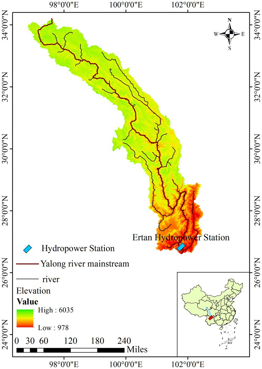
Figure 1. Yalong River Basin.

The Ertan Hydropower Station is situated in the lower reaches of the Yalong River within the Panxi Rift Zone. Its dam controls a catchment area of 11.6 × 10⁴ km² (90.3% of the entire basin), with a mean annual flow of 1,670 m³/s, a total reservoir capacity of 58 × 10⁸ m³, and an installed capacity of 3.3 × 10³ MW. As the first major cascaded development project on the Yalong River, it is situated in the steep transition zone between the Tibetan Plateau and the Yunnan-Guizhou Plateau. The site is in close proximity to the confluence with the Jinsha River, located approximately 33 km away. The station combines large-scale runoff regulation capacity (due to its high dam) with pronounced spatial heterogeneity in hydro- ecological processes characteristic of canyon areas (Xiao et al., 2024).

The data used in this study mainly come from the time series variation mainstream discharge data of the Yalong River monitored by the Ertan Hydropower Station from 2008 to 2013.

2.2 Research method

To address the challenge that seasonal periodic components in runoff series are difficult to capture using ARIMA models, we introduce seasonal terms into the ARIMA framework, constructing a Seasonal Auto Regressive Integrated Moving Average (SARIMA) model for forecasting. The methodological procedure is as follows: First, the original runoff series is decomposed into seasonal, trend, and residual components using the Seasonal-Trend decomposition procedure based on Loess (STL). Second, the SARIMA model is applied separately to forecast each decomposed subsequence, with model parameters optimized through an exhaustive search method. Finally, the predicted values of the trend, seasonal, and residual components are summed to obtain the final runoff forecast (Figure 2).

Figure 2

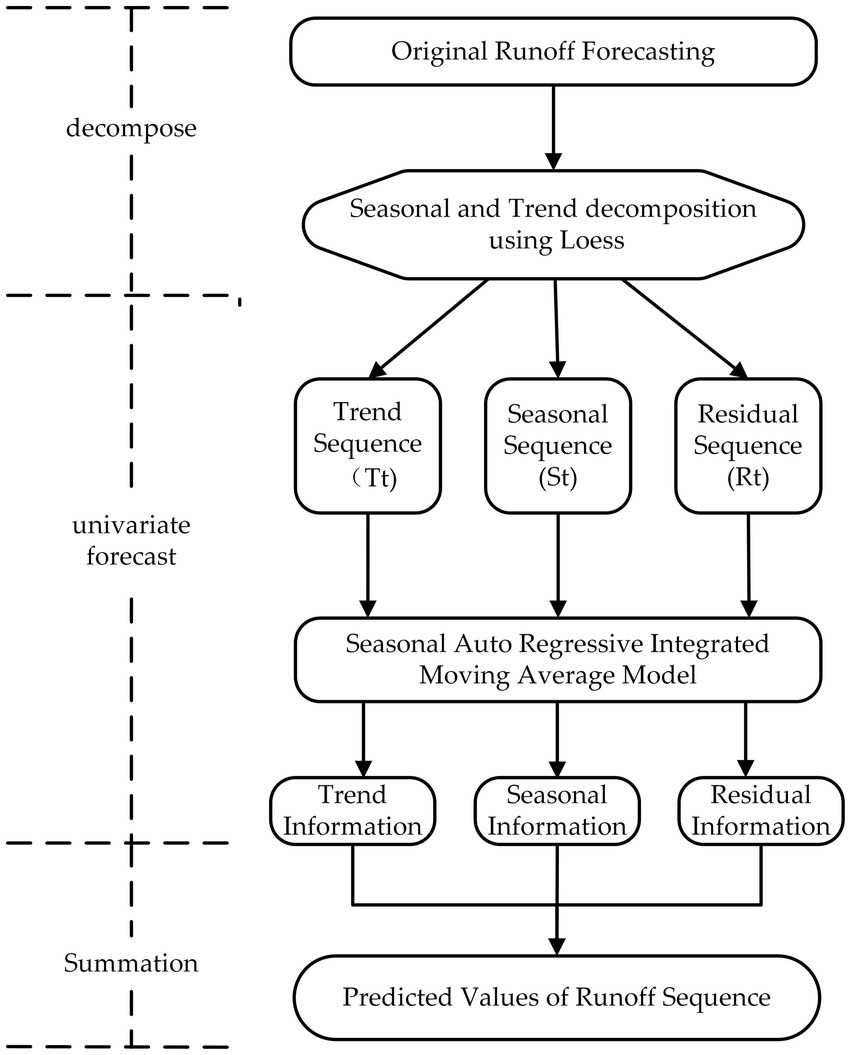
Figure 2. Methodological flowchart.

2.2.1 STL method

The Seasonal-Trend decomposition procedure using Loess (STL) is an exceptionally common and robust time series decomposition method. Compared to other classical seasonal decomposition approaches, STL can handle any type of seasonality and is capable of processing seasonal patterns in data across multiple temporal scales.

For flow data Yt (t = 1, 2, …, n), STL decomposes the original series Yt into seasonal (St), trend (Tt), and residual (Rt) components using locally weighted regression (Luo et al., 2019). The formula (Equation 1) is as follows:

$\begin{array}{ll}{Y}_t=S_t+T_t+R_t& (1)\end{array}$

The STL decomposition consists of two main components: an outer loop and an inner loop. The inner loop is primarily responsible for decomposing the time series into trend (Tt) and seasonal (St) components through iterative smoothing. The outer loop calculates the robustness weights required for the Locally Weighted Scatterplot Smoothing (LOESS) regression in the inner loop. These weights are then applied in the inner loop to reduce the influence of transient anomalies and outliers in the trend and seasonal components.

2.2.2 SARIMA model

The ARIMA (Autoregressive Integrated Moving Average) model primarily consists of three components: the autoregressive (AR) model, the differencing (I) process, and the moving average (MA) model (Khan et al., 2025). SARIMA (Seasonal Autoregressive Integrated Moving Average) extends the ARIMA framework by incorporating seasonal parameters to account for periodicity explicitly tied to temporal cycles (e.g., daily, monthly, or annual patterns) (Singh and Choudhary, 2025). Seasonality refers to systematic variations in data that recur at fixed intervals associated with specific time points. In SARIMA, the seasonal parameter (m) corresponds to the number of observations per seasonal cycle and is predetermined based on data characteristics. For instance, m = 7 denotes a weekly cycle (7 days), m = 12 represents monthly seasonality (12 months/year), and m = 52 indicates a weekly cycle across a year (52 weeks/year).

As illustrated in Figure 3, the hydrological data exhibit pronounced seasonal patterns, justifying the adoption of SARIMA for modeling.

Figure 3

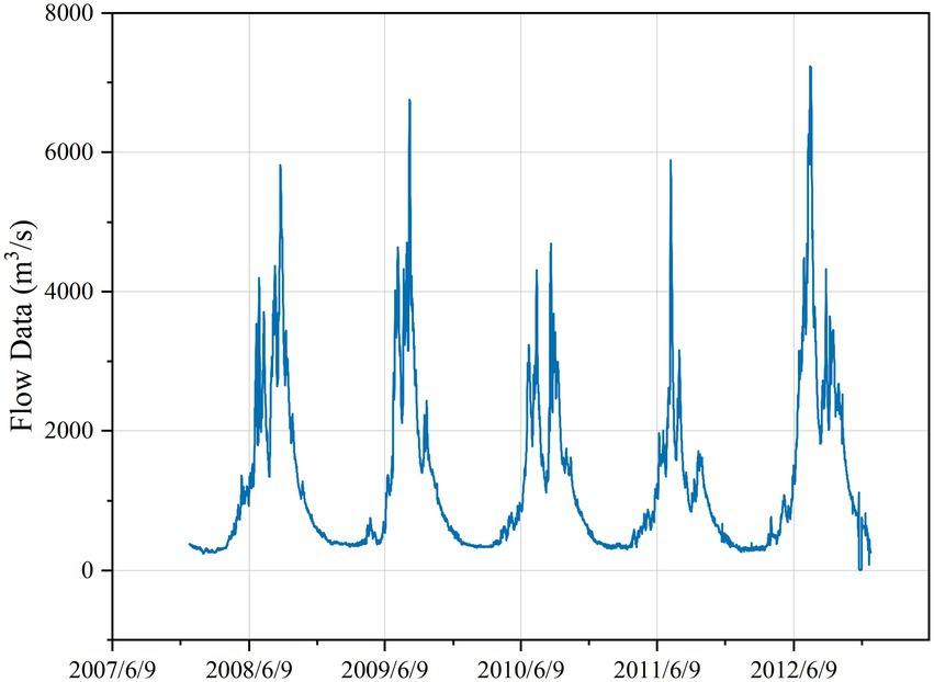
Figure 3. Discharge data chart of one hydrological station.

The standard expression for an ARIMA model is denoted as ARIMA (p, d, q), while the SARIMA model is expressed as SARIMA (p, d, q) (P, D, Q) [m], where uppercase letters represent the seasonal components of the model and lowercase letters represent the non-seasonal components. Here, p and q denote the orders of autoregression and moving average respectively, d indicates the number of non-seasonal differences, P and Q represent the seasonal autoregressive and moving average orders, D signifies the number of seasonal differences, and m stands for the seasonal period length (Parviz and Ghorbanpour, 2024). The mathematical formulation of the SARIMA (p, d, q) (P, D, Q) [m] model (Equation 2) can be expressed as:

$\{\begin{array}{c}\Phi \left(B\right){\nabla }^d{x}_t=\Theta \left(B\right){\in }_t\\ E\left({\in }_t\right)=0,\mathit{Var}\left({\in }_t\right)={\sigma }_{{\in }_t}^2\\ E\left(x_t{\in }_s\right)=0,\forall s<t\end{array},E({\in }_t{\in }_s)=0,s\ne t\text{ (2)}$

Where ${\nabla }^d={(1-B)}^d,\Phi \left(B\right)=1-{\varphi }_{1}B-\cdots -{\varphi }_p{B}^p$ is the autoregressive (AR) polynomial of a stationary and invertible ARMA (p, q) model, and $\Theta \left(B\right)=1-{\theta }_{1}B-\cdots -{\theta }_p{q}^q$ is the moving average (MA) polynomial of the same model (Valipour et al., 2013).

The relevant model parameters were set as follows: the initial values of both p and q were set to 2, with an upper limit of 5; the initial values of both P and Q were set to 1, with an upper limit of 2; and the value of D was set to 1, with an upper limit of 10.

2.2.3 Exhaustive search optimization method

During the SARIMA model forecasting process, an exhaustive search optimization method was employed to determine the optimal parameters (p, d, q) and (P, D, Q). This approach fits the best model to the time series based on information criteria (AIC, AICc, BIC, or HQIC), with Akaike’s Information Criterion (AIC) selected in this study for model evaluation (Martínez-Acosta et al., 2020).

Under given constraints, the algorithm systematically searches across possible non-seasonal and seasonal orders, selecting the parameter combination that minimizes the chosen metric (AIC). The detailed search procedure is illustrated in Figure 4.

Figure 4

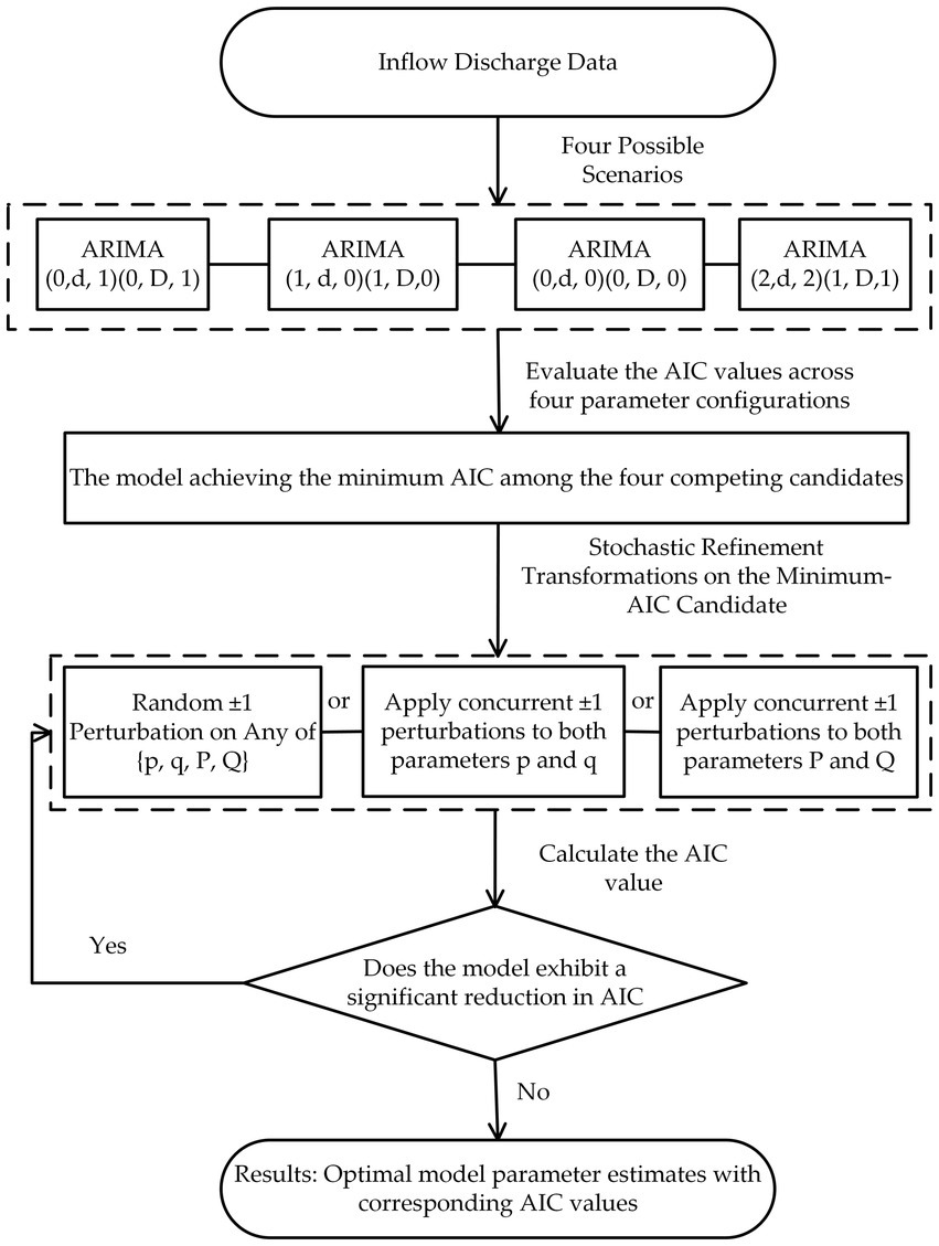
Figure 4. Flowchart of the exhaustive search optimization method.

The Akaike Information Criterion (AIC) is a statistical measure for evaluating the goodness-of-fit of models. In its general form, the AIC (Equation 3) can be expressed as:

$\begin{array}{ll}\mathit{AIC}=2k-2ln\left(L\right)& (3)\end{array}$

Where k is the number of estimated parameters in the model, L is the maximized value of the likelihood function.

2.2.4 Model evaluation metrics

This study fitted a model using the flow data from Ertan Hydropower Station from 2008 to 2011 and tested the model’s predictive effectiveness with the flow data from 2012. The model’s fitting and predictive performance were evaluated using the Root Mean Squared Error (RMSE).

RMSE is one of the most commonly used metrics for evaluating the accuracy of predictive models. It quantifies the deviation between predicted values and actual observations by calculating the square root of the average squared differences (Valipour et al., 2013; Yaseen et al., 2019). The formula (Equation 4) is as follows:

$\begin{array}{ll}\mathit{\text{RMSE}}=\sqrt{\frac{1}{n}\sum _{i=1}^n{(y_i-{\widehat{y}}_i)}^2}& (4)\end{array}$

Where $y_i$ are observed (true) values, ${\widehat{y}}_i$ are predicted values, n is the number of samples (Latif et al., 2024).

3 Results and analysis

3.1 STL time series decomposition results

The STL model was constructed, and through a process of parameter tuning, a seasonal period of 24 was found to yield the best decomposition results, as shown in Figure 5. The trend component exhibits an overall variation pattern consistent with the original runoff series, but with significantly smoother fluctuations, more effectively representing the long-term directional behavior of the runoff sequence. The seasonal component displays clear periodicity, though the amplitude of its oscillations varies with the magnitude of flood seasons. The residual component derived from the runoff series demonstrates a random distribution, with notable increases during annual flood seasons. No discernible patterns were observed in the residuals. It is noteworthy that the residual component exhibits greater variance and uncertainty during the flood season (Figure 5). This amplification can likely be attributed to the high intensity and short duration of rainfall events and the associated rainfall-runoff processes, which exhibit strong stochasticity and nonlinearity. These complex phenomena are not fully captured by the deterministic trend and seasonal components and are thus retained in the residuals. This phenomenon highlights a limitation of the proposed hybrid model: its predictive uncertainty increases under extreme hydrological conditions.

Figure 5

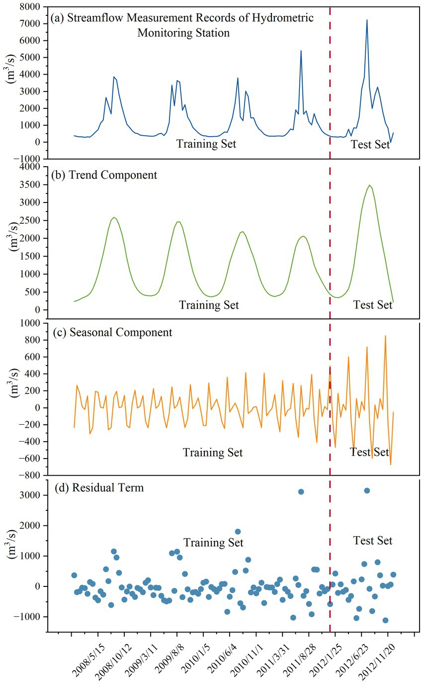
Figure 5. STL time series decomposition results. (a) Streamflow Measurement Records of Hydrometric Monitoring Station (b) Trend Component (c) Seasonal Component (d) Residual Term.

3.2 Runoff prediction results

Due to the limited volume of available data, it was partitioned into a training set and a test set, with 80% allocated to the training set and 20% to the test set (Figure 5).

The ARIMA model and SARIMA model were used to predict the original data and the three decomposed sequences. The optimal performance was achieved by the STL-SARIMA hybrid approach (Figure 6). The root mean square error (RMSE) for the trend component prediction was 834.35, for the seasonal component prediction it was 347.70, and for the residual component prediction it was 877.51. The overall prediction RMSE was 1374.07. The optimal parameters for SARIMA prediction of the original flow data were SARIMA (3,0,0) (1,1,0) _[12], with a RMSE of 1462.65. The model parameters for ARIMA prediction of the original flow data were ARIMA (2,0,0) (0,0,0), with a RMSE of 1664.57. Compared to the three prediction methods, the error values obtained by using SARIMA model prediction with the data after STL decomposition were 6.06% lower than those obtained by directly predicting the original flow data, and 17.45% lower than those obtained by using the ARIMA model to predict the original flow data.

Figure 6

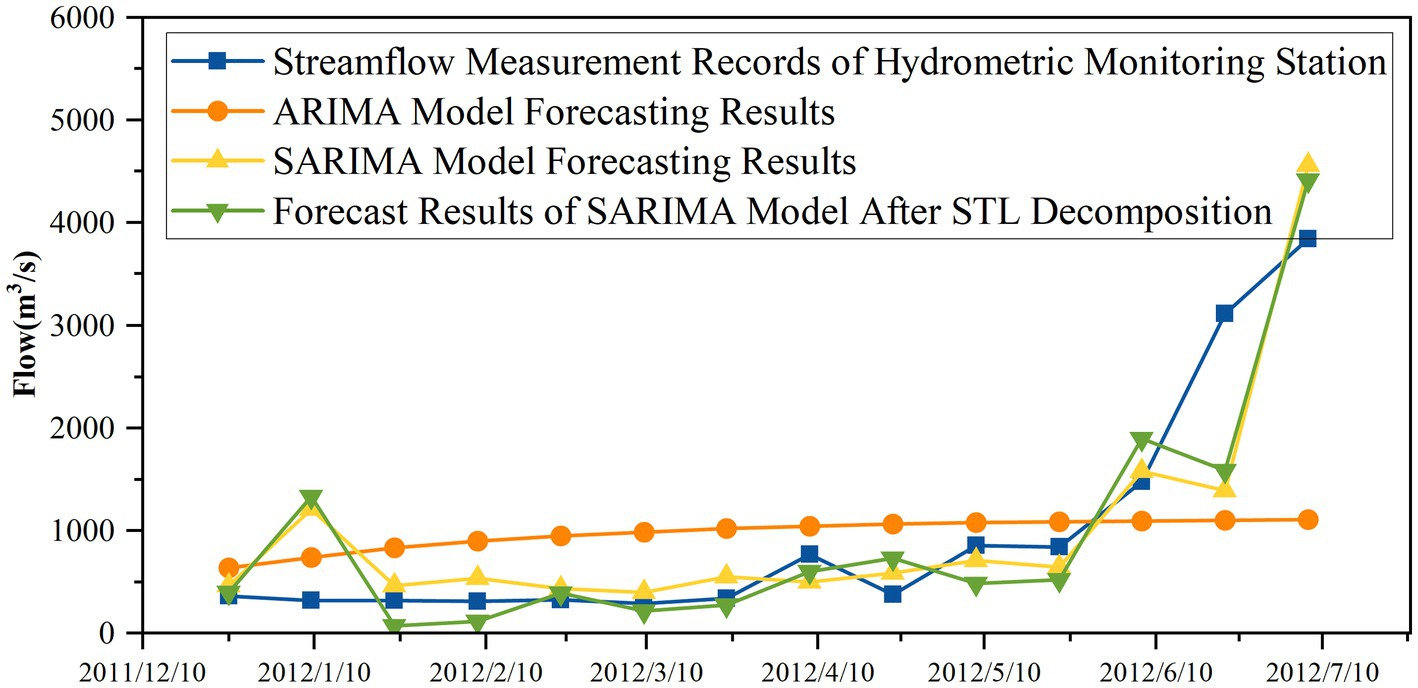
Figure 6. Comparative results of three prediction methods.

4 Discussion

STL decomposition can extract trend and seasonal components from the original series. The trend component likely embodies the aggregated long-term effects of both climate change and human activities. The STL-SARIMA model developed in this study is designed primarily to describe and predict non-stationary series under such combined influences, rather than to strictly attribute contributions to individual driving factors. It demonstrates a satisfactory ability to capture regular seasonal variations resulting from reservoir operations; however, its capability to respond to abrupt and irregular human interventions, such as emergency flood discharge, may be limited. This is a common constraint among data-driven models. Future research could focus on integrating external variables, such as reservoir operation rules and precipitation forecasts, to further improve predictive performance (Yan et al., 2023).

The hydrological flow data inherently exhibit distinct seasonal characteristics, which conventional ARIMA models often fail to adequately capture. The prediction performance showed moderate improvement after incorporating seasonal parameters (SARIMA model). However, the most significant accuracy enhancement was achieved through STL decomposition, which separates the time series into seasonal, trend, and residual components prior to modeling.

Through random sampling of the seasonal parameter m within the range [0, 50], variations in m can significantly impact SARIMA model performance. From the test results, we selected the optimal parameter set yielding minimal error, as illustrated in Figure 7. The seasonal parameter m = 12 was identified as producing the lowest RMSE value. It can be seen that the impact of m on the model is not a linear relationship but rather there is an optimal value, which will infinitely approach the optimal value as it is continuously adjusted.

Figure 7

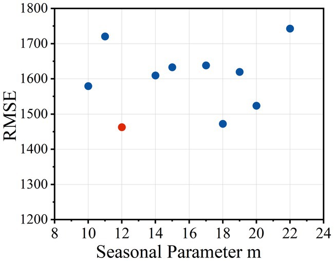
Figure 7. Root mean square error (RMSE) comparison for various parameter settings.

A comparison of prediction results using different seasonal parameters (Figure 8) revealed systematic deviations when validated against hydrometric station flow data. All model configurations exhibited consistent errors in predicting maximum flow values. However, the optimal model performed well during the prediction phase from December 2011 to June 2012, which is related to the characteristics of the SARIMA model itself. The SARIMA model has limitations in predicting nonlinear sequences. Due to the nonlinear characteristics and complex processes of the runoff sequence, no model or algorithm can achieve perfect prediction results. Uncertainty always exists in the modeling process. Therefore, in subsequent research, models suitable for predicting nonlinear sequences, such as Long Short Term Memory Network (LSTM), should also be considered.

Figure 8

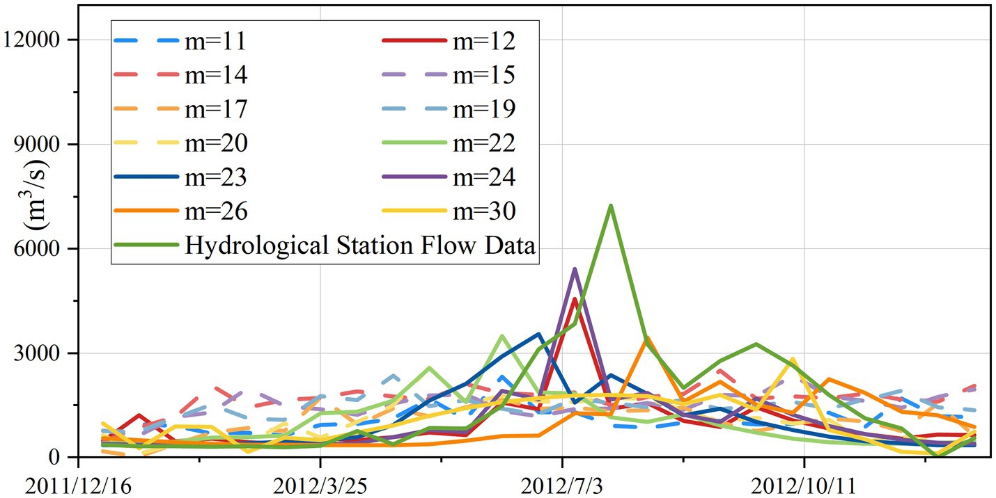
Figure 8. Predictive performance across seasonal parameter settings.

The original time series was normalized by scaling the data to the range [0, 1] before decomposition and forecasting. The formula (Equation 5) is as follows:

$\begin{array}{ll}{X}_{\mathit{norm}}=\frac{X-X_{\min }}{X_{\max }-X_{\min }}& (5)\end{array}$

Where X is the original data value, X_min and X_max are the minimum and maximum values in the dataset, respectively, and X_norm is the normalized value.

To facilitate comparison with predictions from non-normalized data, the forecasted values were inverse-normalized to their original scale before error computation. Normalization significantly reduced prediction errors compared to raw data forecasting (Figure 9). This improvement was observed regardless of whether STL decomposition was applied, confirming that normalization independently enhances forecast accuracy (Bouach, 2024) (Figure 10). Normalization improved computational efficiency during model optimization. It accelerated the identification of the optimal seasonal parameter (m) due to stabilized gradient dynamics in parameter search algorithms.

Figure 9

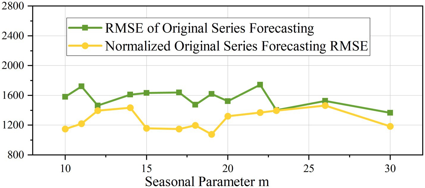
Figure 9. Performance comparison between normalized and non-normalized series.

Figure 10

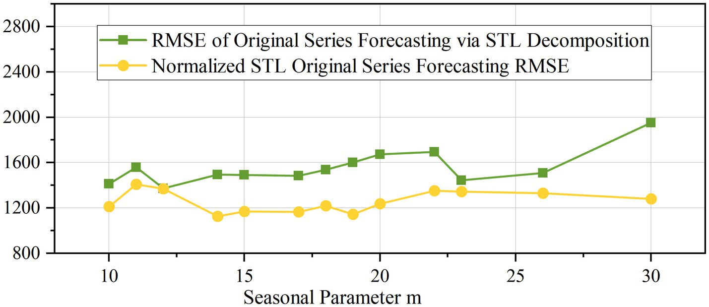
Figure 10. Performance comparison between STL-decomposed original series and normalized series.

5 Conclusion

This study developed a hybrid runoff forecasting model integrating time series decomposition with SARIMA modeling. The runoff characteristics of the Ertan Hydropower Station in the Yalong River Basin were analyzed and simulatively predicted using observed data from 2008 to 2013. The main research conclusions are as follows:

Analysis of STL-decomposed runoff data from Ertan Hydropower Station reveals: The trend component maintains close alignment with the original runoff series while demonstrating enhanced smoothness; The seasonal component exhibits distinct periodicity, with its oscillation amplitude modulated by flood season discharge magnitude; The residual component lacks discernible patterns but displays significant amplification during annual flood seasons.

The proposed STL-SARIMA model in this study addresses limitations of conventional forecasting approaches, including low prediction accuracy, poor interpretability, and difficulty in capturing seasonal components. This hybrid framework achieves enhanced forecasting precision while maintaining straightforward modeling procedures. The RMSE of the STL-SARIMA model prediction result is 1,374.07, demonstrating a 6.06% reduction in error compared to the standalone SARIMA model and a 17.45% reduction relative to the standalone ARIMA model.

The seasonal parameter m significantly influences SARIMA model predictions, with the minimal RMSE achieved at m = 12. However, persistent deviations between predicted maxima and observed values indicate inherent limitations of SARIMA in forecasting nonlinear sequences. Thus, subsequent refinement of the methodology necessitates incorporating models specifically designed for nonlinear sequence prediction.

Normalizing the original data sequence improves the accuracy of the SARIMA model. The results obtained from STL decomposition and SARIMA model prediction on normalized data are optimal.

Data availability statement

The raw data supporting the conclusions of this article will be made available by the authors, without undue reservation.

Author contributions

YK: Conceptualization, Data curation, Writing – original draft. YX: Funding acquisition, Writing – review & editing. WW: Data curation, Software, Writing – review & editing. TL: Writing – review & editing. XZ: Funding acquisition, Writing – review & editing. GW: Project administration, Writing – review & editing. LQ: Writing – review & editing.

Funding

The author(s) declare that financial support was received for the research and/or publication of this article. This study was financially supported by the National Key Research and Development Program of China (grant no. 2023YFC3006501), the National Natural Science Foundation of China (grant nos. 42075191 and 52009080).

Conflict of interest

The authors declare that the research was conducted in the absence of any commercial or financial relationships that could be construed as a potential conflict of interest.

Generative AI statement

The authors declare that no Gen AI was used in the creation of this manuscript.

Any alternative text (alt text) provided alongside figures in this article has been generated by Frontiers with the support of artificial intelligence and reasonable efforts have been made to ensure accuracy, including review by the authors wherever possible. If you identify any issues, please contact us.

Publisher’s note

All claims expressed in this article are solely those of the authors and do not necessarily represent those of their affiliated organizations, or those of the publisher, the editors and the reviewers. Any product that may be evaluated in this article, or claim that may be made by its manufacturer, is not guaranteed or endorsed by the publisher.

References

Almeida, T. A. B., Boaventura, L. C. S., Silva, M. V., Farias, C. W. L. A., Chagas, A. M. S., Costa, R. S., et al. (2025). Assessing shallow groundwater depth and electrical conductivity in the Brazilian semiarid: a geostatistical analysis. Geosciences 15:136. doi: 10.3390/geosciences15040136

Crossref Full Text | Google Scholar

Blöschl, G., Bierkens, M. F. P., Chambel, A., Cudennec, C., Destouni, G., Fiori, A., et al. (2019). Twenty-three unsolved problems in hydrology (UPH) - a community perspective. Hydrol. Sci. J. 64, 1141–1158. doi: 10.1080/02626667.2019.1620507

Crossref Full Text | Google Scholar

Bouach, A. (2024). Artificial neural networks for monthly precipitation prediction in north-West Algeria: a case study in the Oranie-chott-Chergui basin. J. Water Clim. Chang. 15, 582–592. doi: 10.2166/wcc.2024.494

Crossref Full Text | Google Scholar

Cleveland, R. B., and Cleveland, W. S. (1990). STL: a seasonal-trend decomposition procedure based on loess. J. Off. Stat. 6:1.

Google Scholar

Dabral, P. P., and Murry, M. Z. (2017). Modelling and forecasting of rainfall time series using sarima. Environ. Process. 4, 399–419. doi: 10.1007/s40710-017-0226-y

Crossref Full Text | Google Scholar

Deman, V. M. H., Koppa, A., Waegeman, W., MacLeod, D. A., Bliss Singer, M., and Miralles, D. G. (2022). Seasonal prediction of horn of Africa long rains using machine learning: the pitfalls of preselecting correlated predictors. Front. Water 4:1053020. doi: 10.3389/frwa.2022.1053020

Crossref Full Text | Google Scholar

Dimri, T., Ahmad, S., and Sharif, M. (2020). Time series analysis of climate variables using seasonal Arima approach. J. Earth Syst. Sci. 129:16. doi: 10.1007/s12040-020-01408-x

Crossref Full Text | Google Scholar

Dong, S.-H., Zhou, H.-C., and Xu, H.-J. (2004). A forecast model of hydrologic single element medium and long-period based on rough set theory. Water Resour. Manag. 18, 483–495. doi: 10.1023/B:WARM.0000049180.27315.12

Crossref Full Text | Google Scholar

Fathian, F., Mehdizadeh, S., Sales, A. K., and Safari, M. J. S. (2019). Hybrid models to improve the monthly river flow prediction: integrating artificial intelligence and non-linear time series models. J. Hydrol. 575, 1200–1213. doi: 10.1016/j.jhydrol.2019.06.025

Crossref Full Text | Google Scholar

Ha, S., Liu, D. R., and Mu, L. (2021). Prediction of Yangtze River streamflow based on deep learning neural network with el nino-southern oscillation. Sci. Rep. 11:23. doi: 10.1038/s41598-021-90964-3

Crossref Full Text | Google Scholar

Hyndman, R. J., and Khandakar, Y. (2008). Automatic time series forecasting: the forecast package for R. J. Stat. Softw. 27, 1–22. doi: 10.18637/jss.v027.i03

Crossref Full Text | Google Scholar

Khan, M. M., Sarwar, M. K., Zafar, M. A., Rashid, M., Tariq, M. A. U. R., Haider, S., et al. (2025). Comparative analysis of inflow forecasting using machine learning and statistical techniques: case study of Mangla reservoir and Marala headworks. Front. Environ. Sci. 13:1590346. doi: 10.3389/fenvs.2025.1590346

Crossref Full Text | Google Scholar

Latif, S. D., Mohammed, D. O., and Jaafar, A. (2024). Developing an innovative machine learning model for rainfall prediction in a semi-arid region. J. Hydroinf. 26, 904–914. doi: 10.2166/hydro.2024.014

Crossref Full Text | Google Scholar

Li, J. T., Ai, P., Xiong, C. S., and Song, Y. H. (2025). Leveraging multi-source data and teleconnection indices for enhanced runoff prediction using coupled deep learning models. Sci. Rep. 15:27. doi: 10.1038/s41598-025-00115-1

Crossref Full Text | Google Scholar

Liu, Z. Z., Cai, Y. L., Meng, S. L., Zhu, Z. Z., Meng, X. L., Wang, X. L., et al. (2025). Global forecasting of atmospheric CO₂ concentrations using a hybrid STL-prophet-LSTM model. Int J Sust Dev World 32, 498–508. doi: 10.1080/13504509.2025.2490667

PubMed Abstract | Crossref Full Text | Google Scholar

Liu, D. R., Jiang, W. C., Mu, L., and Wang, S. (2020). Streamflow prediction using deep learning neural network: case study of Yangtze River. IEEE Access 8, 90069–90086. doi: 10.1109/access.2020.2993874

Crossref Full Text | Google Scholar

Luo, X. G., Yuan, X. H., Zhu, S., Xu, Z. Y., Meng, L. S., and Peng, J. (2019). A hybrid support vector regression framework for streamflow forecast. J. Hydrol. 568, 184–193. doi: 10.1016/j.jhydrol.2018.10.064

Crossref Full Text | Google Scholar

Madushani, J. A. T., Withanage, N. C., Mishra, P. K., Meraj, G., Kibebe, C. G., and Kumar, P. (2025). Thematic and bibliometric review of remote sensing and geographic information system-based flood disaster studies in South Asia during 2004–2024. Sustainability 17:217. doi: 10.3390/su17010217

Crossref Full Text | Google Scholar

Martínez-Acosta, L., Medrano-Barboza, J. P., López-Ramos, A., López, J. F. R., and López-Lambraño, A. A. (2020). Sarima approach to generating synthetic monthly rainfall in the Sinu River watershed in Colombia. Atmos. 11:602. doi: 10.3390/atmos11060602

Crossref Full Text | Google Scholar

Parviz, L., and Ghorbanpour, M. (2024). A hybrid EMD and MODWT models for monthly precipitation forecasting using an innovative error decomposition method. Stoch. Environ. Res. Risk Assess. 38, 4107–4130. doi: 10.1007/s00477-024-02797-x

Crossref Full Text | Google Scholar

Patakchi Yousefi, K., Belleflamme, A., Goergen, K., and Kollet, S. (2024). Impact of deep learning-driven precipitation corrected data using near real-time satellite-based observations and model forecast in an integrated hydrological model. Front. Water 6:1439906. doi: 10.3389/frwa.2024.1439906

Crossref Full Text | Google Scholar

Pechlivanidis, I. G., Du, Y. H., Bennett, J., Boucher, M. A., Chang, A. Y. Y., Crochemore, L., et al. (2025). Enhancing research-to-operations in hydrological forecasting: innovations across scales and horizons. Bull. Am. Meteorol. Soc. 106, E894–E919. doi: 10.1175/bams-d-24-0322.1

Crossref Full Text | Google Scholar

Rather, S. A., Patel, M., and Kapoor, K. (2025). AI-driven forecasting of river discharge: the case study of the Himalayan mountainous river. Earth Sci. Inform. 18:19. doi: 10.1007/s12145-025-01737-9

Crossref Full Text | Google Scholar

Singh, S. K., and Bárdossy, A. (2012). Calibration of hydrological models on hydrologically unusual events. Adv. Water Resour. 38, 81–91. doi: 10.1016/j.advwatres.2011.12.006

Crossref Full Text | Google Scholar

Singh, H., and Choudhary, M. P. (2025). Rainfall prediction in the context of climate change in Thar Desert India using machine learning algorithms. Theor. Appl. Climatol. 156:347. doi: 10.1007/s00704-025-05592-y

Crossref Full Text | Google Scholar

Szatten, D., Łaszyca, E. Z., Bosino, A., De Amicis, M., and Obodovskyi, O. (2025). Impact of climate conditions on the sensitivity of long-term annual river flow in a cascade-dammed river system: the Brda River case study (Poland). Geosciences 15:197. doi: 10.3390/geosciences15060197

Crossref Full Text | Google Scholar

Tang, T. T., Jiao, D. L., Chen, T., and Gui, G. (2022). Medium- and long-term precipitation forecasting method based on data augmentation and machine learning algorithms. IEEE J. Sel. Top. Appl. Earth Obs. Remote Sens. 15, 1000–1011. doi: 10.1109/jstars.2022.3140442

Crossref Full Text | Google Scholar

Tongal, H., and Booij, M. J. (2018). Simulation and forecasting of streamflows using machine learning models coupled with base flow separation. J. Hydrol. 564, 266–282. doi: 10.1016/j.jhydrol.2018.07.004

Crossref Full Text | Google Scholar

Valipour, M., Banihabib, M. E., and Behbahani, S. M. R. (2013). Comparison of the Arma, Arima, and the autoregressive artificial neural network models in forecasting the monthly inflow of dez dam reservoir. J. Hydrol. 476, 433–441. doi: 10.1016/j.jhydrol.2012.11.017

Crossref Full Text | Google Scholar

Wang, H. R., Gao, X., Qian, L. X., and Yu, S. (2012). Uncertainty analysis of hydrological processes based on Arma-garch model. Sci. China-Technol. Sci. 55, 2321–2331. doi: 10.1007/s11431-012-4909-3

Crossref Full Text | Google Scholar

Wittenberg, H., and Sivapalan, M. (1999). Watershed groundwater balance estimation using streamflow recession analysis and baseflow separation. J. Hydrol. 219, 20–33. doi: 10.1016/s0022-1694(99)00040-2

Crossref Full Text | Google Scholar

Xiao, Y., He, L., Chen, X., He, Z., Lai, Y., Luo, F., et al. (2024). Impacts of large hydropower projects on the ecological environment of watersheds: a case study of Ertan reservoir area. Sustainability 16:9125. doi: 10.3390/su16209125

Crossref Full Text | Google Scholar

Xu, W. X., Chen, J., and Corzo, G. (2025). Combining data augmentation and hybrid modeling approaches for deep learning-based monthly streamflow forecasting. J. Hydrol. 659:16. doi: 10.1016/j.jhydrol.2025.133318

Crossref Full Text | Google Scholar

Yan, L., Lei, Q., Jiang, C., Yan, P., Ren, Z., Liu, B., et al. (2022a). Climate-informed monthly runoff prediction model using machine learning and feature importance analysis. Front. Environ. Sci. 10:1049840. doi: 10.3389/fenvs.2022.1049840

Crossref Full Text | Google Scholar

Yan, L., Lu, D., Hu, P., Yan, P., Xu, Y., Qi, J., et al. (2022b). Estimation of design precipitation in Beijing–Tianjin–Hebei region under a changing climate. Hydrol. Sci. J. 67, 1722–1739. doi: 10.1080/02626667.2022.2080554

Crossref Full Text | Google Scholar

Yan, L., Lu, D., Xiong, L., Wang, H., Luan, Q., Jiang, C., et al. (2023). Derivation of nonstationary rainfall intensity-duration-frequency curves considering the impacts of climate change and urbanization. Urban Clim. 52:101701. doi: 10.1016/j.uclim.2023.101701

Crossref Full Text | Google Scholar

Yan, L., Zhang, Y., Zhang, M., and Lall, U. (2025). A nonstationary daily and hourly analysis of the extreme rainfall frequency considering climate teleconnection in coastal cities of the United States. Atmos. 16:75. doi: 10.3390/atmos16010075

Crossref Full Text | Google Scholar

Yaseen, Z. M., Sulaiman, S. O., Deo, R. C., and Chau, K. W. (2019). An enhanced extreme learning machine model for river flow forecasting: state-of-the-art, practical applications in water resource engineering area and future research direction. J. Hydrol. 569, 387–408. doi: 10.1016/j.jhydrol.2018.11.069

Crossref Full Text | Google Scholar

Yavuz, V. S. (2025). Forecasting monthly rainfall and temperature patterns in Van Province, Türkiye, using Arima and sarima models: a long-term climate analysis. J. Water Clim. Chang. 16, 800–818. doi: 10.2166/wcc.2025.798

Crossref Full Text | Google Scholar

Zhang, L., Wang, H., Guo, B., Xu, Y., Li, L., and Xie, J. (2023). Integrated model and application of non–stationary runoff based on time series decomposition and machine learning. Adv. Water Sci. 34, 42–52. doi: 10.14042/j.cnki.32.1309.2023.01.005

Crossref Full Text | Google Scholar

Zhang, Q., Wang, B. D., He, B., Peng, Y., and Ren, M. L. (2011). Singular spectrum analysis and Arima hybrid model for annual runoff forecasting. Water Resour. Manag. 25, 2683–2703. doi: 10.1007/s11269-011-9833-y

Crossref Full Text | Google Scholar

Zhang, J., Yang, M., Dong, N., and Wang, Y. (2025). Machine-learning-based ensemble prediction of the snow water equivalent in the upper Yalong River basin. Sustainability 17:3779. doi: 10.3390/su17093779

Crossref Full Text | Google Scholar

Zhao, T., Zhang, C., Tian, Y., Li, Y., Chen, Z., and Chen, X. (2024). Research progresses and prospects of catchment hydrological forecasting driven by global climate forecasts. Adv. Water Sci. 35, 156–166. doi: 10.14042/j.cnki.32.1309.2024.01.014

Crossref Full Text | Google Scholar