Modelling minimum night consumption as a function of long-run average outflow to users and applications to real world case studies

As accurate monitoring and mitigation of water leakage are essential in the context of smart and resilient cities, this paper proposes a novel methodology for modelling users’ minimum night consumption (MNC), a key parameter in the estimation of district leakage levels. Unlike traditional models, which relate MNC to the number of users supplied by the network district, a new model with a bounded and more interpretable coefficient is conceived to introduce and evaluate the dependence of MNC on the yearly average user outflow, which can be evaluated based on long-run aggregate billed consumption. A methodology is proposed to characterize MNC starting from smart metering data of hourly user water consumption, which are progressively aggregated and analysed at the hour of minimum consumption for the district. Applications to three case studies in Italy, each with distinct characteristics, demonstrate that the novel methodology is beneficial. In fact, the results show that the linear model expressing MNC as a function of the yearly average user outflow fits data better than the traditional model, at increasing aggregation levels.

1 Introduction

Water Distribution Networks (WDNs) are critical infrastructures, ensuring continuous supply of safe and adequate water to users, and drinking water availability is nowadays considered both a global development goal and a human right (Jeandron et al., 2019). However, due to aging infrastructure and external stressors (i.e., increasing water demands due to urban population growth, financial constraints, low maintenance conditions), WDNs are facing frequent component failures (Diao et al., 2016; Mottahedin et al., 2024a), which pose increasing challenges for a sustainable water management (Straus et al., 2016). These challenges include water leakage, which adds up to more than 30% of water withdrawn from sources, with peaks of roughly 60% in critically aged and/or poorly maintained systems. It is estimated that approximately 240,000 water main breaks occur each year in the United States, resulting in the loss of over 2 million gallons of drinking water per day (ASCE, 2017). The global volume of non-revenue water is estimated to be 126 billion cubic meters per year, with a water loss cost adding up to USD 39 billion annually (Liemberger and Wyatt, 2019). Accordingly, water leakage represents a global concern and a crucial aspect to address, since its negative effects are manifold, ranging from the impact on public health to the growth of management cost and end-users’ dissatisfaction due to supply disruption (Lo Presti et al., 2024). As a result, the issue of leakage in WDNs is a priority objective and its reliable estimation is accordingly of paramount importance for prioritizing maintenance and rehabilitation activities, improving allocation of economic resources (Boatwright et al., 2023; Mottahedin et al., 2024b) and selecting the most suitable solution/technology to apply under budget constraints (García et al., 2006).

Various methods are typically adopted for leakage estimation (Amoatey et al., 2018) at the level of district metered area (DMA), which is a hydraulically discrete area within a zone of the WDN for facilitating management. The first and more conventional method is typically applied on long time horizons, one or more years (Marzola et al., 2022). It is based on the comparison between total water volume input into the DMA and billed water volume at DMA users. More modern methods exist, which are capable of identifying leakage based on shorter time horizons, such as days. As an example, the principal component analysis (Duzinkiewicz et al., 2008; Niu et al., 2017; Park et al., 2019; Fezai et al., 2021) can be applied to analyse inflows of DMAs for the identification of outliers, potentially associated with the presence of leakage. Alternatively, leakage can be estimated based on the comparison between minimum night flow (MNF) and minimum night consumption (MNC) in the DMA, both of which typically occur at nighttime between 2:00 and 5:00 a.m. In this time window, users’ activity and water consumption are generally limited, therefore leaving the larger share of the water inflow into the DMA to leakage. Whereas MNF is measured by data derived from flow meters installed at DMA boundary pipes, MNC is usually evaluated by using a simple linear model, expressing this variable as a function of the number of users supplied by the DMA. As MNC is highly dependent on socio-demographic (e.g., property type, household size, daily habits, etc.), technical (e.g., pressure) and climatic (Loureiro et al., 2009; Amoatey et al., 2018; Cominola et al., 2023) factors, the scientific literature reports various values for the coefficient of this linear model, representing the MNC for the single DMA user: 1.7 L/user/h in the UK (Butler, 2009), 3 L/user/h for Canada, 5 L/user/h for Malaysia (Fantozzi and Lambert, 2012), 2.8 L/user/h or 4 L/user/h in Italy, while excluding or including the post-meter leakage, respectively, (Alassio et al., 2024), 1 L/user/h for Germany and 2 L/user/h for Austria (Fantozzi and Lambert, 2012). As to non-residential users, Fantozzi and Lambert (2012) suggest a simplified value of 8 L/user/h for all activities, though Butler (2009) reports specific values ranging between 0.9 and 20.5 L/user/h, depending on the kind of commercial activity.

Despite the various worthy scientific contributions listed above, the issue of MNC assessment is far from being fully understood, calling for new experimental and numerical works. In fact, the large variability in the MNC observed so far in the scientific literature gives water utility managers great uncertainty in the application of the MNC method in different contexts from those analysed in the past. Therefore, new experiments can help mitigate this uncertainty and give the MNC method more trustworthiness for leakage estimation. On the other hand, the question arises if other models can be used for MNC estimation in a more reliable way as opposed to the conventional models relating MNC to the number of users.

This paper aims to bridge the two research gaps mentioned above. From an experimental standpoint, it enriches the available database with two additional case studies from Italy, by analysing both residential and non-residential users (the available studies for the latter are very limited in literature). In this context, it makes use of data derived from smart metering technology, which is spreading and offering numerous benefits in WDN management e.g., (see Cominola et al., 2015; Fiorillo et al., 2020; Mazzoni et al., 2023) and modelling (Cardell-Oliver, 2013; Clifford et al., 2018; Cominola et al., 2019; Giudicianni et al., 2022). From a numerical standpoint, it proposes an entirely new modelling paradigm, in which MNC is no longer evaluated as a function of the number of DMA users, but rather as a function of the long-run average of the aggregate user outflow, which can be evaluated based on users’ billed consumption.

The remainder of the paper is organized as follows. The next section presents the methodology adopted, followed by applications (case studies and results) and conclusions, highlighting the advantages of the novel approach and presenting prospects of future work.

2 Materials and methods

The methodology used in this work is based on the exploitation of the hourly series of consumption of DMA users, hereinafter indicated as outflow to users. Preliminarily to the application of the methodology, users are subdivided into two categories, namely residential and non-residential, and the respective average daily patterns of hourly consumption are investigated. At this stage, no treatment of outliers is performed and hourly series are analysed on a yearly basis, without delving into the effects of seasonality within the single year. Overall, the methodology develops in the following steps:

1. Identification of the minimum consumption time (MCT, i.e., the hour at which consumption is lowest) for the whole DMA.

2. Characterization of each user in terms of MNC (L/h) at the MCT, for both user categories.

3. Aggregation of the users in either category, and determination of the aggregate value of MNC, i.e., MNC_agg (L/h), at the MCT and at increasing aggregation steps (obtained by adding one user at a time).

4. Construction of the linear model expressing MNC_agg as a function of the aggregate number of users N_u (−), or of the yearly average aggregate consumption Q_agg (L/h), i.e., the sum of the yearly average outflow to users, obtained as is shown in Equation 1:

$\begin{array}{ll}{\mathrm{Q}}_{\mathrm{agg}}={\sum }_{\mathrm{i}=1}^{{\mathrm{N}}_{\mathrm{u}}}{\mathrm{Q}}_{\mathrm{i}}& (1)\end{array}$

in which Q_i (L/h) is the hourly average outflow Q to the i-th user.

The conventional linear model relating MNC_agg to N_u takes on the form shown in Equation 2:

$\begin{array}{ll}{\mathrm{MNC}}_{\mathrm{agg}}=\alpha {\mathrm{N}}_{\mathrm{u}}& (2)\end{array}$

with α being the coefficient of the model with units of measurement L/h.

The novel linear model relating MNC_agg to Q_agg takes on the form shown in Equation 3:

$\begin{array}{ll}{\mathrm{MNC}}_{\mathrm{agg}}=\beta {\mathrm{Q}}_{\mathrm{agg}}& (3)\end{array}$

with β being the dimensionless coefficient of the model.

More specifically, the linear structure was selected for the novel model in Equation 3 because it has been widely used in the scientific literature to represent the relationship between MNC and N_u shown in Equation 2 e.g., (see Butler, 2009; Fantozzi and Lambert, 2012; Alassio et al., 2024). Furthermore, this simple structure facilitates practical applications by water utilities.

As to step 3, it is worth noting that users’ aggregation can be carried out with different sorting criteria, leading to different sequences of MNC_agg, with only the first and last elements being the same. In fact, the first and last elements are equal to 0 (no users) and to the MNC_agg value for the full group of users in the DMA, respectively. Then, a graph like the one in Figure 1 can be constructed, in which MNC_agg is plotted against the aggregate number of users N_u or the aggregate consumption Q_agg. In this graph, various MNC_agg(N_u), or MNC_agg(Q_agg) patterns can be considered, including those obtained from random aggregation samples. The envelope including all the potential MNC_agg(N_u), or MNC_agg(Q_agg) patterns is delimited by two boundary lines. The lower line is obtained by considering the aggregation of users sorted based on increasing values of MNC, or MNC/Q. The upper line is obtained by considering the aggregation of users sorted based on decreasing values of MNC, or MNC/Q. Finally, the trend of the linear model (constructed in step 4 based on Equation 2 or Equation 3), associated with the straight line connecting the first and last dots, which are the same for all aggregation sequences, can be plotted on the graph.

Figure 1

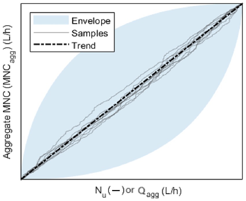
Figure 1. Aggregate MNC_agg as a function of N_u or Q_agg. See section 2 for the description.

Graphs like that in Figure 1 enable analysing and comparing MNC_agg(N_u) and MNC_agg(Q_agg) patterns for both residential and non-residential users.

The goodness-of-fit of the models in Equations 2 and 3 is assessed by means of the average envelope width W (L/h), calculated by dividing the envelope area by the maximum value of the abscissa associated with the envelope. The smaller W, the better the model capability of representing MNC_agg. Additionally, to better evaluate the goodness-of-fit, the R² is also calculated as the square of the correlation coefficient between the pattern of the lower (or upper) boundary line of the envelope and the straight line pattern of either model. The minimum of these two R² values is the lowest value obtainable in the aggregation of users. The closer R² to 1, the better the model capability of representing MNC_agg.

3 Applications

3.1 Case studies

In this section, the residential and non-residential users’ water consumption data are described for three Italian case studies (see the general view in Figure 2), indicated as Case Study A (CSA), Case Study B (CSB) and Case Study C (CSC), respectively. In all the case studies, both kinds of users belong to the urban context. More specifically, residential users include domestic water consumers, whereas non-residential users include typical urban non-domestic contexts (e.g., restaurants, shops, commercial activities, small factories, and so forth).

Figure 2

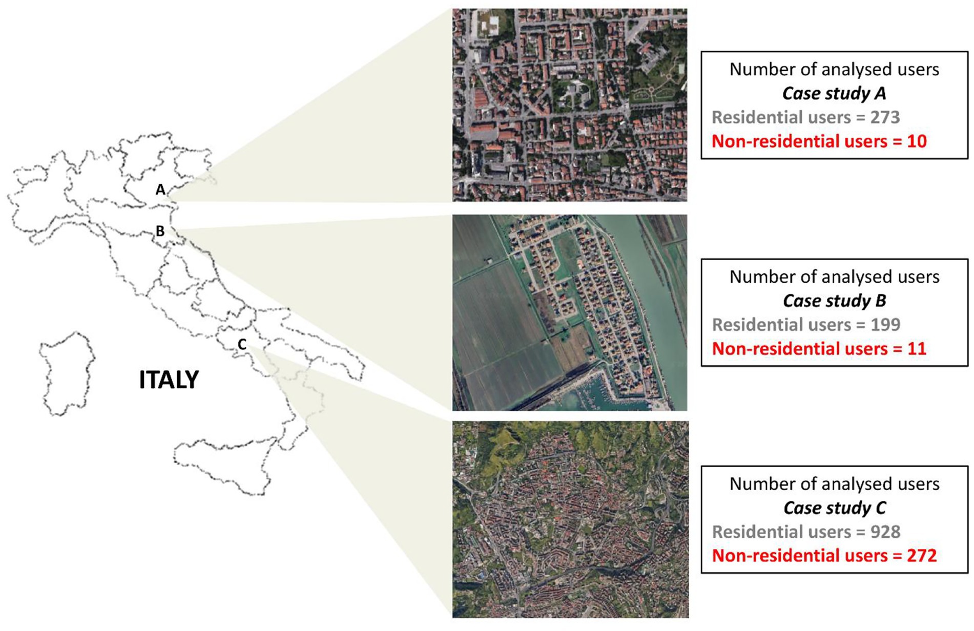
Figure 2. General satellite view of the three (two in Northern Italy and one in Southern Italy) case studies and corresponding number of users analysed.

CSA is a typical urban district, located in the suburb of a medium-sized city in Northern Italy. It includes 273 residential users and 21 non-residential users (i.e., small commercial establishments and catering services). Almost 2 years of data concerning consumption at hourly resolution is available for CSA from May 2019 to March 2021. For the purposes of this work, the data sample of non-residential users was reduced to the pre-COVID period from June 2019 to February 2020. In greater detail, the removal of data from March 2020 to March 2021 enables discarding all data potentially affected by the effects of the pandemic, the outburst of which in Italy was in March 2020, following the first case reported at the end of February 2020. Data were also corrected to exclude post-meter leakages by applying the sliding-window-based approach of Alassio et al. (2024), consisting in the identification of long periods of continuous consumption (i.e., longer than 72 h). Specifically, all residential users and 10 out of 21 non-residential users were finally selected.

CSB is a seaside district with a touristic component in Northern Italy. It includes 199 residential users and 17 non-residential users (mainly related to commercial and catering facilities, as is the case with CSA). Two years of data concerning consumption data at hourly resolution is available for CSB from September 2016 to August 2018. For the purposes of this work, the data sample was reduced to the period from January 2017 to January 2018 and was corrected to exclude post-meter leakage. All residential users and 11 out of 17 non-residential users were finally selected.

CSC is urban district covering the suburban area of a large seaside city in Southern Italy. In this DMA, most traditional water meters (i.e., 4,989 out of 5,380) have recently been replaced with smart meters. One year of data from March 2017 to March 2018 concerning hourly consumption was made available by the water utility for CSC. For the purposes of this work, 928 residential and 272 non-residential users were selected, with no cases of data removal from the data sample due to post-meter leakages.

In all case studies, users included in the analysis were required to have non-zero daily consumption for more than half of the yearly period considered. This ensured the exclusion of fully (or partially) inactive users, as well as those affected by data transmission errors. As a result, purely seasonal users (active only in summer) were excluded from CSB, thereby ensuring the consistency of CSB with the two other case studies.

The graphs in Figure 3 provide insights into the average daily pattern of hourly consumption for residential and non-residential users across the three case studies. The analysis of graphs (a) reveals that the profiles of the mean values for residential users are similar across the three case studies. A typical bimodal pattern is observed, with peaks occurring in the morning and evening. Additionally, CSA and CSB feature a third and less pronounced peak at midday. Overall, consumption variability is higher during periods of increased demand. At each hour, the mean always lies inside the whiskers and is consistently slightly higher than the median, indicating a slight positive skewness.

Figure 3

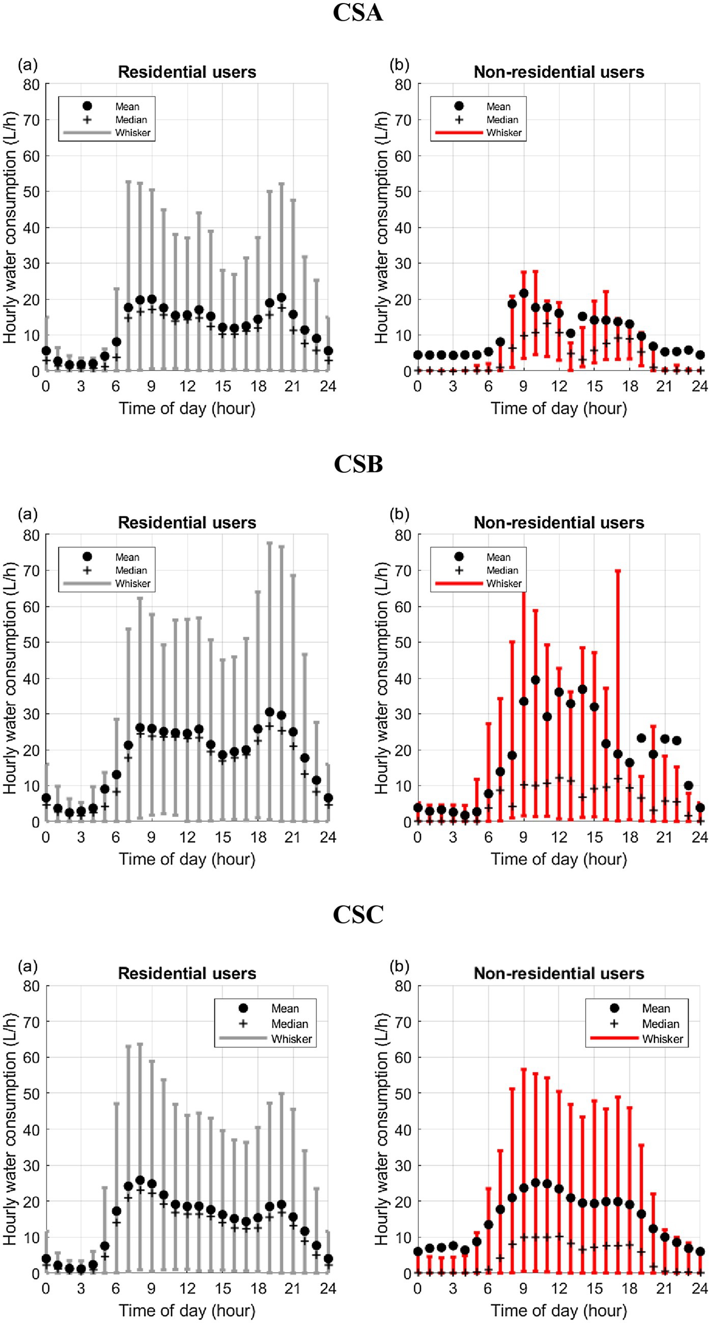
Figure 3. CSA, CSB and CSC. Box-plot graphs showing the daily average pattern of hourly water consumption for (a) residential and (b) non-residential users.

In contrast, the analysis of graphs (b) shows that non-residential users display markedly different patterns, with greater variability across the case studies. The profile of mean values is jagged in CSA and CSB, while it is smoother in CSC, likely due to the larger number of users in this case study. In addition, the distance between the mean and median is more pronounced than in the residential case, revealing a stronger positive skewness. Furthermore, in CSA and CSC, the mean lies outside the whiskers during nighttime hours, influenced by a small number of high-consumption users, representing distribution outliers.

Figure 4 shows the (normalized) daily average aggregate profiles. In all case studies, aggregate daily consumption is heavily dominated by residential users, who represent the primary source of consumption. As a result, the overall profile shapes are similar to the residential patterns observed in panel (a) of Figure 3. Overall, CSA and CSB present similar profiles, with three distinct peaks. Conversely, the profile for CSC shows only two peaks—the former in the morning and the latter, less pronounced, in the evening—alongside a generally declining trend from morning to evening. This divergence between CSA/CSB and CSC may reflect different user habits between Northern and Southern Italy.

Figure 4

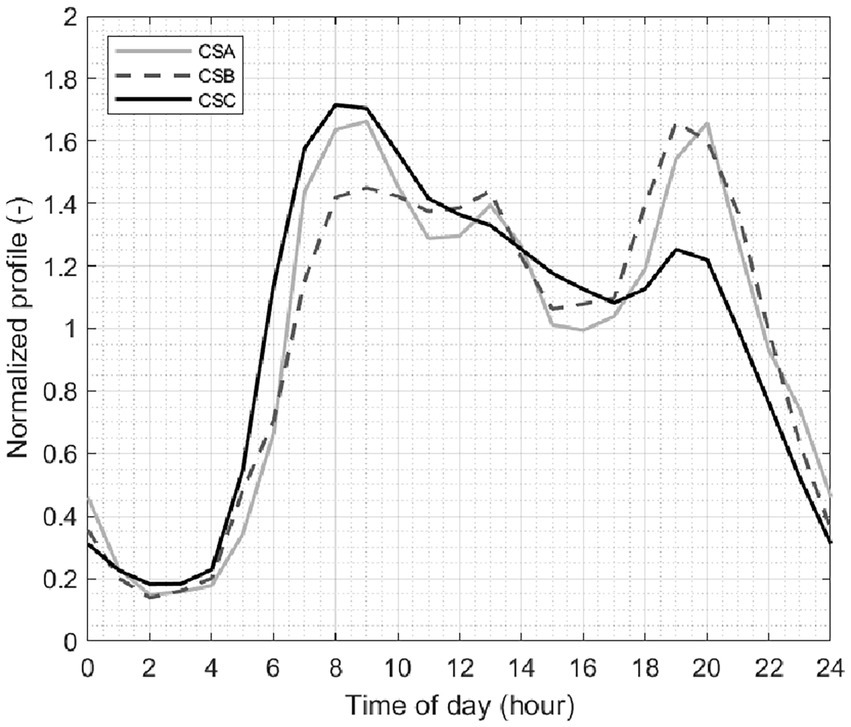
Figure 4. Aggregate water demand patterns in CSA, CSB and CSC.

3.2 Results

The methodology described in section 2 was applied to the three case studies. Calculations were carried out and graphs were constructed by using Matlab® 2024b (The MathWorks Inc, 2024). The MCT was remarked from 2 to 3 a.m. in all the case studies, consistently with the scientific literature (e.g., the night period occurring from 2 to 4 a.m. according to Liemberger and Farley, 2004). The application of the methodology yielded the results shown in Figures 5–7, respectively.

Figure 5

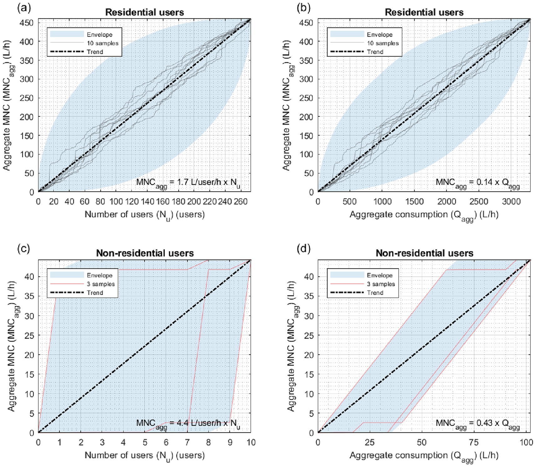
Figure 5. CSA: patterns (a) MNC_agg(N_u) and (b) MNC_agg(Q_agg) for residential users; patterns (c) MNC_agg(N_u) and (d) MNC_agg(Q_agg) for non-residential users.

Figure 6

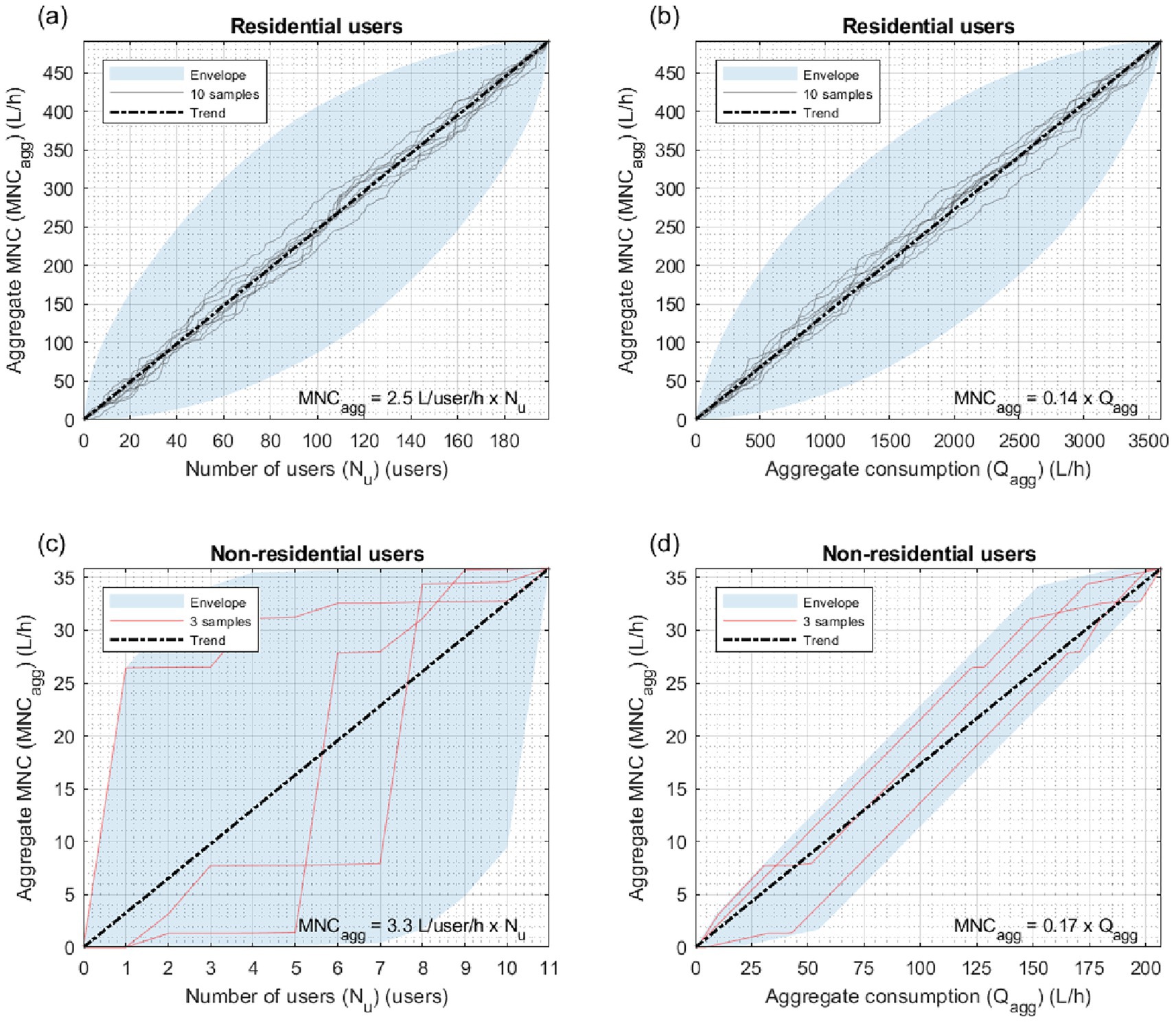
Figure 6. CSB: patterns (a) MNC_agg(N_u) and (b) MNC_agg(Q_agg) for residential users; patterns (c) MNC_agg(N_u) and (d) MNC_agg(Q_agg) for non-residential users.

Figure 7

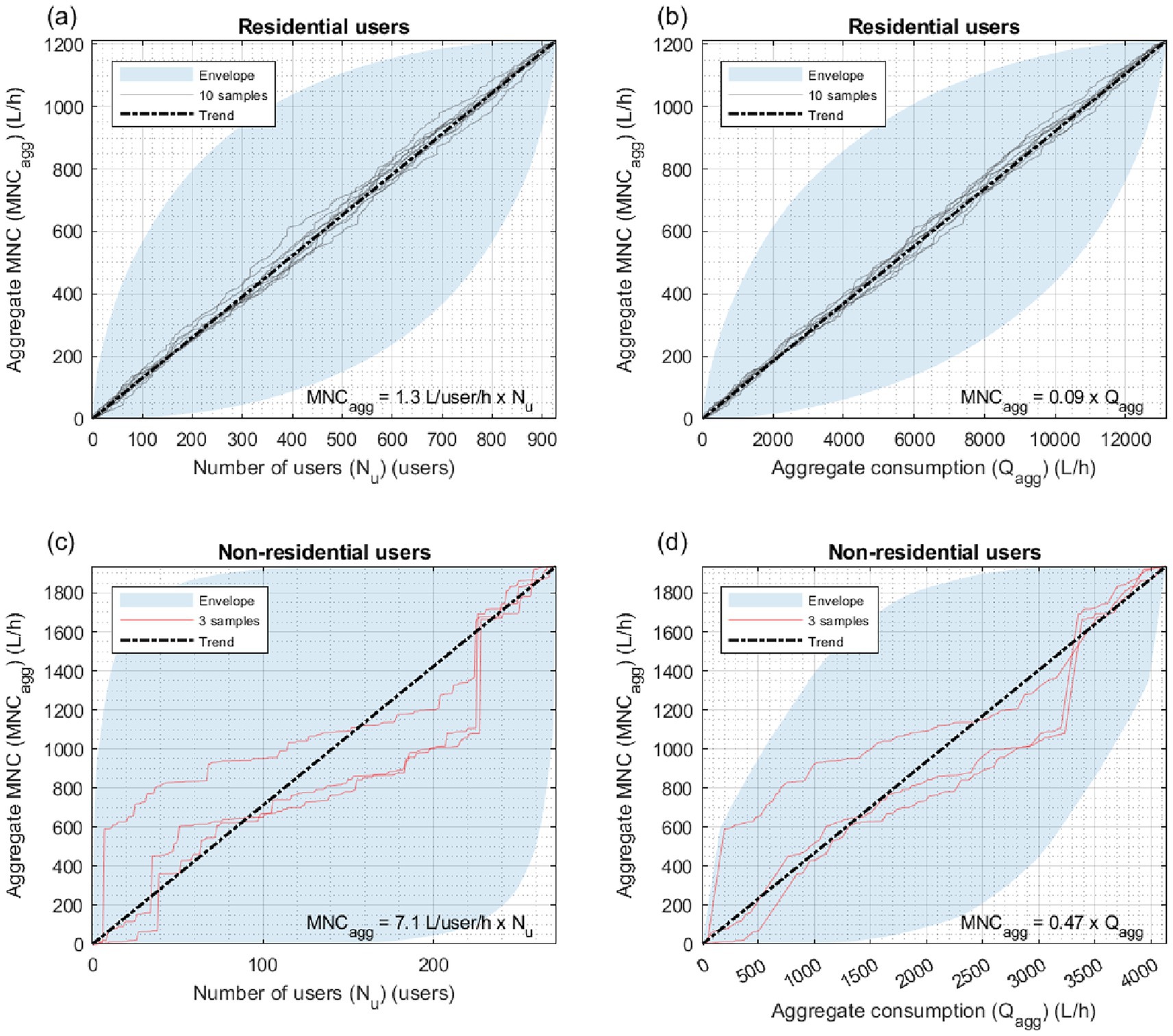
Figure 7. CSC: patterns (a) MNC_agg(N_u) and (b) MNC_agg(Q_agg) for residential users; patterns (c) MNC_agg(N_u) and (d) MNC_agg(Q_agg) for non-residential users.

For CSA, Figure 5a shows MNC_agg as a function of N_u for 10 samples adopted of residential users’ aggregation. It is worth noting that these 10 samples were generated through a random process, that is by randomly selecting the first and all the subsequent elements. At the first step of aggregation, one user is randomly selected among N_u,tot = 273 users; at the second step, the selection is performed from the remaining (N_u,tot-1) users, and so forth; at the i-th step, a user is chosen among the remaining (N_u,tot+1-i) candidates. At the final step, a single remaining user can be selected. Therefore, each generated sample corresponds to one possible of N_u,tot! = 273! permutations. The graph also shows the envelope including all the potential MNC_agg(N_u) patterns obtained by aggregating the residential users in CSA and the trend of the model MNC_agg = 1.7 × Nu, corresponding to the straight line connecting the first and last dots in the aggregation process (model coefficient α = 1.7 considering model structure in Equation 2). Figure 5b shows MNC_agg as a function of Q_agg for the same 10 samples as in Figure 5a, the envelope including all the potential MNC_agg(Q_agg) patterns and the trend of the model MNC_agg = 0.14 × Q_agg, corresponding to the straight line connecting the first and last dots in the aggregation process (model coefficient β = 0.14 considering model structure in Equation 3). The comparison of graphs points out that the envelope is narrower in Figure 5b than in Figure 5a. By calculating the average envelope width W (as explained in section 2), it emerges that W = 253 L/h in Figure 5b is smaller than W = 284 L/h in Figure 5a. This attests to the better regularity of pattern MNC_agg(Q_agg), which results closer to the linear model than pattern MNC_agg(N_u) for the aggregated users. Figures 5c,d extend the same kind of analysis and comparison to non-residential users. For this category, the linear models described in Equations 2 and 3 yield coefficients α and β equal to 4.4 and 0.43, respectively. The better regularity and closeness of pattern MNC_agg(Q_agg) to the linear model is much more evident for the non-residential users, as the envelope average width W = 16 L/h in Figure 5d is much smaller than W = 40 L/h in Figure 5c.

Similar remarks can be made about CSB and CSC based on the results shown in Figures 6 and 7, respectively.

In all the graphs in Figures 5–7, the straight line associated with the linear model is well centred within the envelope of all potential user aggregations for both residential and non-residential users. Despite the variability of the model coefficient values across the three case studies, especially for non-residential users, this attests to the suitability of the linear model also in the cases where the envelope width is large.

The coefficients α and β of the linear models yielded for the residential and non-residential users in the three case studies are summarized in the following Tables 1 and 2, for the models MNC_agg(N_u) and MNC_agg(Q_agg), respectively. The average envelope width W values are reported in Table 3 for both the models MNC_agg(N_u) and MNC_agg(Q_agg). Overall, compared to the model MNC_agg(N_u) shown in Equation 2, the model MNC_agg(Q_agg) shown in Equation 3 enables reducing the average envelope width by a percentage ranging from 7 to 11% for residential users. The percentage reduction for non-residential users goes instead from 28 to 69%. Similar benefits were obtained also in terms of R², as is shown in Table 4.

Table 1

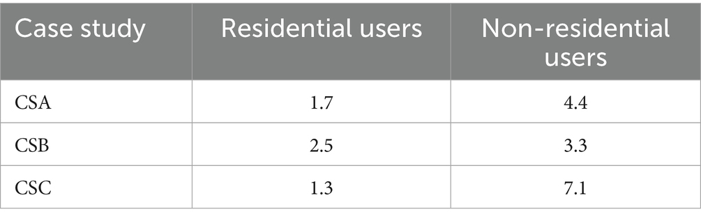
Table 1. Coefficient α for linear models MNC_agg(N_u) (Equation 2) obtained in the three case studies, for residential and non-residential users.

Table 2

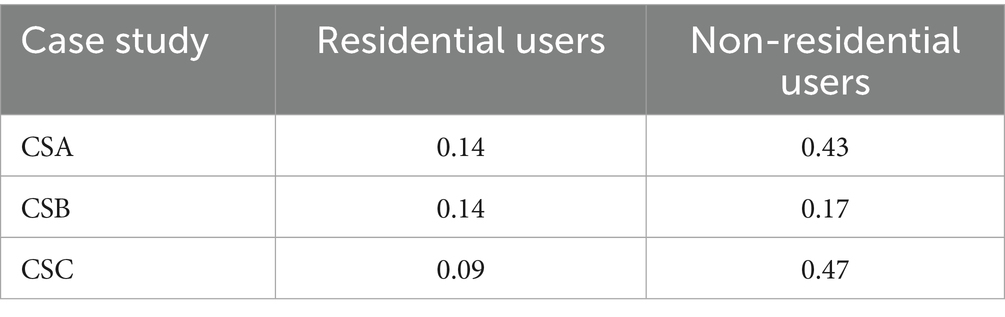
Table 2. Coefficient β for linear models MNC_agg(Q_agg) (Equation 3) obtained in the three case studies, for residential and non-residential users.

Table 3

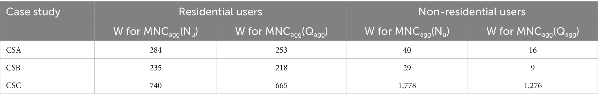
Table 3. Average envelope width W values for linear models MNC_agg(N_u) (Equation 2) and MNC_agg(Q_agg) (Equation 3) obtained in the three case studies, for residential and non-residential users.

Table 4

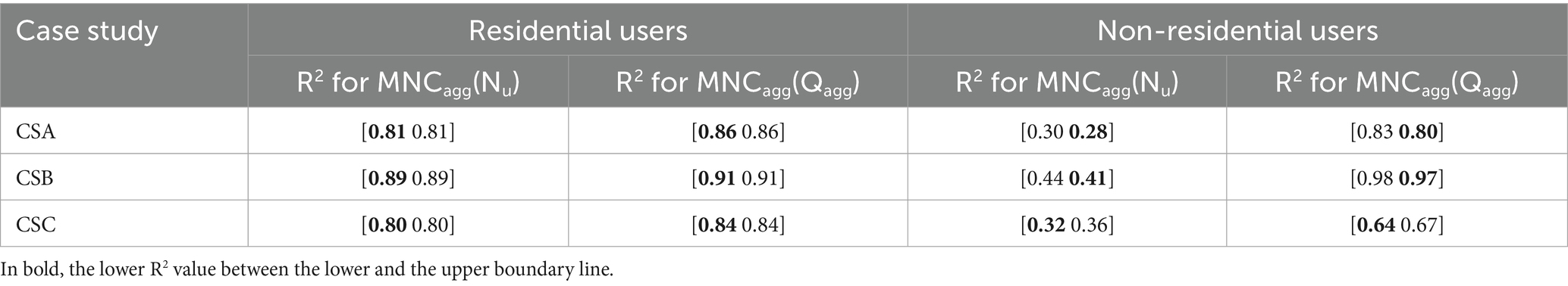
Table 4. R² values as the squares of the correlations between lower/upper envelope boundary line and straight line associated with the model, evaluated for linear models MNC_agg(N_u) (Equation 2) and MNC_agg(Q_agg) (Equation 3) in the three case studies, for residential and non-residential users.

Some comparisons can be performed with studies available in the scientific literature in the context of the model MNC_agg(N_u). First, it is worth noting that the results obtained for CSB are consistent with those reported by Alassio et al. (2024) for the same case study. In fact, in their work focussed only on residential users, the linear model MNC_agg = 2.8 × N_u was obtained by considering a longer smart metering database. However, the coefficient α = 2.8 of this model is close to the value α = 2.5 obtained for residential users in the present study. In all case studies, the coefficient α of the model for residential users falls within the range between 1.7 and 2.5 (Table 1), which is consistent with values commonly reported in the scientific literature (Butler, 2009; Fantozzi and Lambert, 2012; Alassio et al., 2024). For non-residential users, the values of α observed in this study—ranging from 3.3 and 7.1— (Table 1) are consistent with the broader range reported in the literature, spanning from 0.9 to 20.5 (Butler, 2009; Fantozzi and Lambert, 2012).

Table 2 shows that the coefficient β of the linear model MNC_agg(Q_agg) (Equation 3) ranges between 0.09 and 0.14 and between 0.17 and 0.47, for the residential and non-residential users, respectively, revealing higher values for the latter category in this case as well. It is worth noting that the coefficients for residential users are considerably close to each other, attesting to the homogenization capacity of the residential model MNC_agg(Q_agg).

The comparison of Tables 1 and 2 proves that, when expressing MNC_agg as a function of Q_agg, (Equation 3), the range of absolute variation for the coefficient of the linear model is drastically reduced compared to MNC_agg(N_u) (Equation 2). Furthermore, the linear model MNC_agg(Q_agg) is advantageous due to its dimensionless formulation and the better predictability of its coefficient β. Playing the role of demand coefficient relating minimum demand at an hour to average demand, β is constrained to take on values lower than or equal to 1. Indeed, the value of 1 is achieved asymptotically in the theoretical case in which the aggregate user consumption is constant, resulting in the model MNC_agg = Q_agg. Otherwise, the larger the variability in the daily consumption, the farther the coefficient from 1. The bounded nature of the coefficient β of the model MNC_agg(Q_agg) marks a meaningful difference from the coefficient α of the linear model MNC_agg(N_u), which is theoretically unbounded.

4 Discussion and conclusions

In this work, the smart metering data from three Italian case studies with distinct characteristics were analysed and compared, and a novel assessment and characterization was presented for residential and non-residential MNC, to contribute to the existing body of knowledge in WDN demand characterization. Specifically, a methodology based on the statistical analysis of MNC at the hour of minimum consumption for the district at increasing levels of user aggregation was applied to characterize the dependence of MNC on the long-run average aggregate outflow to users, with advantages compared to the conventional approaches expressing MNC as a function of the aggregate number of users. While both MNC and average user outflow were derived in this work from smart meter readings, the yearly average user outflows can be easily obtained from the billed water consumption even in the absence of smart meters.

The main conclusions of this work are the following:

• The linear model for assessing MNC fits data better when it is expressed as a function of the average user outflow, instead of the number of users.

• The benefits in terms of fit can reach values up to about 70%, based on the metric defined and considered for assessing model fit in the present work.

• The novel linear model proposed is more meaningful and elegant, as it simply expresses a minimum value as a function of an average, therefore resulting in a dimensionless coefficient.

• In the linear model based on the average user outflow as independent variable, the coefficient is more easily predictable than in the conventional model with the number of users as independent variable, as its upper bound equal to 1 is known a priori.

• In the considered case studies, a quite small range of values around 0.1 was observed for the model coefficient in the case of residential users, as a result of the homogenization capacity of the novel model.

The better predictability of the coefficient of the novel linear model can provide water utilities with a more reliable estimation of MNC, resulting in the more reliable estimation of leakage as the difference between MNF and MNC in DMAs, and ultimately to achieve more informed budget allocation for leak repair.

The novel model proposed in this work is expected to find widespread applications in technical contexts, due to its advantages and ease of implementation. However, in light of the large variability in MNC estimation results reported in the scientific literature, caution is required when extending the models developed to case studies beyond those described in the present work. Specifically, the range of values obtained for the coefficient of the novel linear model MNC_agg(Q_agg) is relatively narrow in the case of residential users (between 0.09 and 0.14), which may lead to only minor estimation errors when applied to different contexts. In contrast, the coefficient range is wider (between 0.17 and 0.44) for non-residential users, highlighting the need for further investigations aimed at exploring the relationship between this coefficient and the specific type of non-residential activity. For both residential and non-residential users, future endeavours will be necessary to assess the extent to which the coefficient values obtained in this work are valid in other countries than Italy. Acknowledging the uncertainty in non-residential MNC, the model coefficient for districts featuring both residential and non-residential users can be estimated as a weighted average of the respective coefficients, with weights determined based on the daily average aggregate outflows to users. This approach would help mitigate the effects of the large uncertainty associated with non-residential MNC.

Data availability statement

The datasets presented in this study can be found in online repositories. The names of the repository/repositories and accession number(s) can be found at: Giudicianni et al. (2025).

Author contributions

CG: Formal analysis, Investigation, Methodology, Writing – review & editing. FM: Formal analysis, Investigation, Methodology, Writing – review & editing. VM: Formal analysis, Investigation, Methodology, Writing – review & editing. SA: Conceptualization, Formal analysis, Investigation, Methodology, Writing – review & editing. EC: Conceptualization, Formal analysis, Investigation, Methodology, Writing – original draft.

Funding

The author(s) declare that no financial support was received for the research and/or publication of this article.

Acknowledgments

Support from Italian MIUR and University of Pavia is acknowledged within the Dipartimenti di Eccellenza 2023–2027 programme.

Conflict of interest

The authors declare that the research was conducted in the absence of any commercial or financial relationships that could be construed as a potential conflict of interest.

Generative AI statement

The author(s) declare that no Gen AI was used in the creation of this manuscript.

Any alternative text (alt text) provided alongside figures in this article has been generated by Frontiers with the support of artificial intelligence and reasonable efforts have been made to ensure accuracy, including review by the authors wherever possible. If you identify any issues, please contact us.

Publisher’s note

All claims expressed in this article are solely those of the authors and do not necessarily represent those of their affiliated organizations, or those of the publisher, the editors and the reviewers. Any product that may be evaluated in this article, or claim that may be made by its manufacturer, is not guaranteed or endorsed by the publisher.

References

Alassio, S., Marsili, V., Mazzoni, F., and Alvisi, S. (2024). Exploring residential minimum night consumption in a real water distribution network based on smart-meter data. Discov. Water 4:88. doi: 10.1007/s43832-024-00150-5

Crossref Full Text | Google Scholar

Amoatey, P. K., Minke, R., and Steinmetz, H. (2018). Leakage estimation in developing country water networks based on water balance, minimum night flow and component analysis methods. Water Pract. Technol. 13, 96–105. doi: 10.2166/wpt.2018.005

Crossref Full Text | Google Scholar

ASCE (2017). Drinking water report. ASCE infrastructure report card. Reston, VA: ASCE.

Google Scholar

Boatwright, S., Mounce, S., Romano, M., and Boxall, J. (2023). Integrated sensor placement and leak localization using geospatial genetic algorithms. J. Water Resour. Plan. Manag. 149:04023040. doi: 10.1061/JWRMD5.WRENG-6037

Crossref Full Text | Google Scholar

Butler, D. (2009). Leakage detection and management. Cwmbran, UK: Palmer Environmental.

Google Scholar

Cardell-Oliver, R. (2013). Water use signature patterns for analyzing household consumption using medium resolution meter data. Water Resour. Res. 49, 8589–8599. doi: 10.1002/2013wr014458

Crossref Full Text | Google Scholar

Clifford, E., Mulligan, S., Comer, J., and Hannon, L. (2018). Flow-signature analysis of water consumption in nonresidential building water networks using high-resolution and medium-resolution smart meter data: two case studies. Water Resour. Res. 54, 88–106. doi: 10.1002/2017WR020639

Crossref Full Text | Google Scholar

Cominola, A., Giuliani, M., Piga, D., Castelletti, A., and Rizzoli, A. E. (2015). Benefits and challenges of using smart meters for advancing residential water demand modeling and management: a review. Environ. Model. Softw. 72, 198–214. doi: 10.1016/j.envsoft.2015.07.012

Crossref Full Text | Google Scholar

Cominola, A., Nguyen, K., Giuliani, M., Stewart, R. A., Maier, H. R., and Castelletti, A. (2019). Data mining to uncover heterogeneous water use behaviors from smart meter data. Water Resour. Res. 55, 9315–9333. doi: 10.1029/2019WR024897

Crossref Full Text | Google Scholar

Cominola, A., Preiss, L., Thyer, M., Maier, H. R., Prevos, P., Stewart, R. A., et al. (2023). The determinants of household water consumption: a review and assessment framework for research and practice. NPJ Clean Water 6:11. doi: 10.1038/s41545-022-00208-8

Crossref Full Text | Google Scholar

Diao, K., Sweetapple, C., Farmani, R., Fu, G., Ward, S., and Butler, D. (2016). Global resilience analysis of water distribution systems. Water Res. 106, 383–393. doi: 10.1016/j.watres.2016.10.011

PubMed Abstract | Crossref Full Text | Google Scholar

Duzinkiewicz, K., Borowa, A., Mazur, K., Grochowski, M., Brdys, M. A., and Jezior, K. (2008). Leakage detection and localisation in drinking water distribution networks by multiregional PCA. Stud. Inf. Control 17, 135–152.

Google Scholar

Fantozzi, M, and Lambert, AO (2012). “Residential night consumption — assessment, choice of scaling units and calculation of variability.” In Proceedings of the IWA Water Loss Conference, Manila, Philippines, 26–29 February 2012

Google Scholar

Fezai, R., Bouzrara, K., Mansouri, M., Nounou, H., Nounou, M., and Puig, V. (2021). “A novel leak detection approach in water distribution networks.” In: Proceedings of 18th International Multi-Conference on Systems, Signals & Devices (SSD), Monastir, Tunisia, 2021, pp. 607–612.

Google Scholar

Fiorillo, D., Galuppini, G., Creaco, E., De Paola, F., and Giugni, M. (2020). Identification of influential user locations for smart meter installation to reconstruct the urban demand pattern. J. Water Resour. Plan. Manag. 146:04020070. doi: 10.1061/(ASCE)WR.1943-5452.0001269

Crossref Full Text | Google Scholar

García, V. J., Cabrera, E., and Cabrera Jr, E. (2006).” The minimum night flow method revisited.” In Water distribution systems analysis symposium 2006. pp. 1–18.

Google Scholar

Giudicianni, C., Campisano, A., Di Nardo, A., and Creaco, E. (2022). Pulsed demand modeling for the optimal placement of water quality sensors in water distribution networks. Water Resour. Res. 58:e2022WR033368. doi: 10.1029/2022WR033368

Crossref Full Text | Google Scholar

Giudicianni, C., Mazzoni, F., Marsili, V., Alvisi, S., and Creaco, E. (2025). Data from three Italian sites for minimum night consumption (MNC) evaluation. Figshare. [Dataset]. Available at: https://figshare.com/articles/dataset/Data_from_three_Italian_sites_for_minimum_night_consumption_MNC_evaluation/29219879. doi: 10.6084/m9.figshare.29219879.v1

Google Scholar

Jeandron, A., Cumming, O., Kapepula, L., and Cousens, S. (2019). Predicting quality and quantity of water used by urban households based on tap water service. NPJ Clean Water 2:23. doi: 10.1038/s41545-019-0047-9

Crossref Full Text | Google Scholar

Liemberger, R, and Farley, M. (2004). “Developing a non-revenue water reduction strategy: investigating and assessing water losses.” In Proceedings of the IWA 4th World Water Congress, Marrakech, Morocco, 19–24 September 2004.

Google Scholar

Liemberger, R., and Wyatt, A. (2019). Quantifying the global non-revenue water problem. Water Supply 19, 831–837. doi: 10.2166/ws.2018.129

Crossref Full Text | Google Scholar

Lo Presti, J., Giudicianni, C., Toffanin, C., Creaco, E., Magni, L., and Galuppini, G. (2024). Combining clustering and regularised neural network for burst detection and localization and flow/pressure sensor placement in water distribution networks. J Water Process Eng 63:105473. doi: 10.1016/j.jwpe.2024.105473

Crossref Full Text | Google Scholar

Loureiro, D, Borba, R, Rebelo, M, Alegre, H, Coelho, ST, Covas, DIC, et al. (2009). “Analysis of household night-time consumption. Integrating water systems”. in Proceedings of the 10th International on Computing and Control for the Water Industry.

Google Scholar

Marzola, I., Mazzoni, F., Alvisi, S., and Franchini, M. (2022). Leakage detection and localization in a water distribution network through comparison of observed and simulated pressure data. J. Water Resour. Plan. Manag. 148:04021096. doi: 10.1061/(ASCE)WR.1943-5452.0001503

Crossref Full Text | Google Scholar

Mazzoni, F., Alvisi, S., Franchini, M., and Blokker, E. J. M. (2023). Exploiting high-resolution data to investigate the characteristics of residential water consumption at the end-use level: a Dutch case study. Water Resour. Ind. 29:10019. doi: 10.1016/j.wri.2022.100198

PubMed Abstract | Crossref Full Text | Google Scholar

Mottahedin, A., Giudicianni, C., Brentan, B., and Creaco, E. (2024b). Clustering-based maintenance strategy of isolation valves in water distribution networks. ACS ES&T Water 4, 1798–1807. doi: 10.1021/acsestwater.3c00793

Crossref Full Text | Google Scholar

Mottahedin, A., Giudicianni, C., Di Nunno, F., Granata, F., Cunha, M., Walski, T., et al. (2024a). Analysis, design, and maintenance of isolation valves in water distribution networks: state of the art review, insights from field experiences and future directions. Water Res. 262:122088. doi: 10.1016/j.watres.2024.122088

Crossref Full Text | Google Scholar

Niu, Z., Wang, C., Zhang, Y., Wei, X., and Gao, X. (2017). Leakage rate model of urban water supply networks using principal component regression analysis. Trans. Tianjin Univ. 24, 172–181. doi: 10.1007/s12209-017-0090-x

Crossref Full Text | Google Scholar

Park, S., Ha, J., and Kim, K. (2019). The principal component analysis for detecting leaks in water pipe networks utilizing flow and leak record data. Desalin. Water Treat. 143, 69–77. doi: 10.5004/dwt.2019.23375

Crossref Full Text | Google Scholar

Straus, J., Chang, H., and Hong, C. Y. (2016). An exploratory path analysis of attitudes, behaviors and summer water consumption in the Portland metropolitan area. Sustain. Cities Soc. 23, 68–77. doi: 10.1016/j.scs.2016.03.004

Crossref Full Text | Google Scholar

The MathWorks Inc (2024). MATLAB version: 24.2.0.2923080 (R2024b). Natick, Massachusetts: The MathWorks Inc.

Google Scholar