Abstract
Based on field investigations in multiple irrigation districts, it was found that farmers frequently employ sandbag barriers or direct pumping to meet irrigation demands, disrupting irrigation schedules and destabilizing downstream water supply. The core issue stems from differential deterioration of canal sections after prolonged operation, causing variations in Manning’s roughness coefficient and seepage rates. Consequently, irrigation plans based on historical experience no longer satisfy water-level accuracy requirements. This study focuses on a typical canal system in the Ningxia Yellow River Irrigation District, utilizing the NSGA-II optimization algorithm to simultaneously calibrate Manning’s roughness coefficient and seepage parameters. The results indicate that Manning’s roughness exhibits significant spatial heterogeneity in canal sections constructed with the same technique after several years of operation; the simulated values at three water level control sections generally align with the measured trends, with absolute water level errors within 0.03 m; through accurate parameter identification and combined with AMR adaptive mesh refinement technology, the canal flow process is precisely simulated, enabling timely irrigation schedule adjustments to resolve the aforementioned conflicts.; by assessing canal section deterioration and prioritizing anti-seepage measures, corn irrigation area is projected to expand by over 3.2 hectares. This research holds significant practical value for enhancing water resource utilization efficiency, boosting agricultural productivity, and advancing sustainable development in irrigation districts. Future efforts could integrate water inflow predictions, crop water requirements, and coordinated control of gate groups to establish a digital twin-driven precision irrigation framework for the entire canal system.
1 Introduction
Irrigation canal systems serve as a critical link between water sources and farmlands, playing a key role in enhancing irrigation efficiency. The accurate simulation of flow processes and the efficient operation of these systems are essential for agricultural water resources management (Khaeez and Hashemy Shahdany, 2021; Fan et al., 2023). However, the precision of canal flow simulation is often constrained by the accurate calibration of key hydraulic parameters, such as the Manning’s roughness coefficient and the seepage coefficient (Zhou et al., 2023). Traditional methods largely rely on empirical lookup tables or simple empirical formulas for estimating roughness (Aricò et al., 2009), which often fail to adequately capture the spatial variability of parameters, thereby limiting the practical applicability of these models in real-world irrigation systems.
In recent years, with the widespread application of optimization algorithms in hydraulic parameter inversion, various methods have been proposed to improve the identification accuracy of the Manning’s roughness coefficient. For instance, some studies have combined heuristic search with clustering algorithms to identify the spatial distribution patterns of roughness in natural rivers (Attari and Hosseini, 2019; Attari et al., 2021); others have utilized neural networks for the dynamic inversion of Manning’s coefficient in unsteady open channel flows (Zevallos et al., 2025; Li et al., 2025); and some have modeled the overall flow resistance coefficient and composite roughness coefficient for complex canal conditions (Ryu et al., 2025). In terms of seepage calculation, research approaches mainly include experimental measurements (such as the static water method), empirical formulas (Alam and Bhutta, 2004; Lund et al., 2023), and three-dimensional modeling for seepage calculation in lined canals (Han et al., 2021; Han et al., 2022). Although these methods have made significant progress in roughness identification and seepage calculation, most still treat roughness and seepage as independent issues, neglecting their synergistic effects and parameter interactions in flow simulation. Such artificial decoupling can easily lead to error propagation and model distortion, limiting the applicability of these methods in actual irrigation scenarios.
To address the aforementioned limitations, this study introduces the multi-objective evolutionary algorithm NSGA-II to establish a novel calibration framework capable of simultaneously inverting the Manning’s roughness coefficient and the seepage parameter. As a classic multi-objective optimization algorithm, NSGA-II has demonstrated significant advantages in handling high-dimensional, nonlinear, and conflicting objectives in parameter inversion across various fields (Kong et al., 2025; Deng et al., 2025; Abkar et al., 2025). Building upon a systematic review of existing optimization methods, this research integrates traditional seepage formulas into the Saint-Venant equations. Utilizing 864 sets of water level and flow observation data from the Han-Yan Canal in Ningxia, the NSGA-II algorithm is employed to achieve synchronous global optimization of multiple parameters. Furthermore, sensitivity analysis is incorporated to effectively quantify parameter interactions, thereby significantly enhancing the physical consistency and numerical robustness of the inversion results. The main contributions of this paper are summarized as follows:
-
Methodological Innovation: Proposes a novel approach for identifying channel roughness and seepage parameters based on the NSGA-II algorithm, utilizing measured water level and flow data to achieve simultaneous multi-parameter calibration. This advances from single-parameter, step-by-step calibration to multi-objective, collaborative inversion, with parameter sensitivity analysis conducted to investigate inter-parameter relationships.
-
Technical Improvement: Integrates optimized calibration results with Adaptive Mesh Refinement (AMR) technology to enhance the accuracy of channel flow simulation, providing a reliable basis for irrigation scheduling.
-
Application Breakthrough: Combines parameter calibration outcomes with field investigation results to scientifically assess the deterioration condition of each canal segment through a dual-factor evaluation system. Compared to traditional large-scale reconstruction, this approach supports targeted rehabilitation and optimized fund allocation, facilitating the dual goals of water conservation in irrigation districts and increased agricultural productivity.
2 Materials and methods
2.1 Research site and measured data
Ningxia Hui Autonomous Region, located between 35°14′–39°23′N and 104°17′–107°39′E, lies deep in the northwestern inland plateau. Characterized by a typical continental semi-humid to semi-arid climate, it serves as a crucial grain production base. The Hanyan Canal, situated in Ningxia Hui Autonomous Region of the People’s Republic of China, was initially constructed in 200 BC—over two millennia ago. Through subsequent continued construction and modernization efforts, it has evolved into a large-scale modern irrigation district with a main canal stretching 88 km and a commanded irrigated area of approximately 50 million mu (approximately 33,333.33 hectares). Its annual water diversion capacity reaches about 5 hundred million cubic meters, with a maximum design diversion flow of 80 cubic meters per second. The star symbol in Figure 1 indicates the canal segment at the Fourth Management Station of the Hanyan Canal, which serves as the study focus of this paper. From left to right, the marked locations correspond to the Tongqiao flow measurement section, Changfeng Canal, Changzhong Canal, and Zhangyi Canal, labeled as Sections D1, D2, D3, and D4, respectively. The canal segments between these sections are sequentially designated as Reach S1, S2, and S3. The total length of the studied segment is 2,904 m. The data were collected in May 2020 and May 2021. The Section D1 dataset comprises flow measurement data provided by the Fourth Management Station of Hanyan Canal for water settlement purposes. The water level and flow data for Sections D2, D3, and D4 were recorded by integrated measurement and control gates (Figure 2), with automatic recordings taken at 5-min intervals. The parameters of the gate incorporating integrated measurement and control are shown in Table 1.
Figure 1

Study area and field photos.
Figure 2

Metering equipment (integrated flow measurement and control gates).
Table 1
| Parameter | Specification/description |
|---|---|
| Sensor type | Ultrasonic water level gauge; Acoustic matrix flowmeter (16-sensor pairs) |
| Measurement principle | Ultrasonic ranging; Flow is calculated by 3D segmentation of the water column via an acoustic matrix and summation of the segments. |
| Water level accuracy | ±0.1 mm |
| Flow rate accuracy | Laboratory conditions: ≤±2.5%; Field conditions: ≤±5% |
| Installation location | Offtake of branch canals |
| Installation context | The channel bed was concreted and leveled to ensure stable measurement conditions and consistent flow regime. |
Parameters for integrated measurement and control gates.
2.2 Mathematical model
In unsteady flow modeling, the selection of model dimensionality requires a trade-off between computational efficiency and simulation accuracy. While high-dimensional models can precisely describe complex flow patterns and energy conversion processes, they involve complicated governing equations and high computational costs (Aricò et al., 2007; Almeida et al., 2012). This study focuses on regularly-shaped lined canals and adopts the one-dimensional Saint-Venant equations for flow simulation. This model features a simple structure, fewer parameters, and high computational efficiency, making it more practical and economical while maintaining the accuracy required for canal operation and management. Measured water level and flow data from May 4 to 5, 2021 were used as the calibration dataset, data from May 6 as Test Set 1, and data from May 9, 2020 as Test Set 2. The data were complete and collected during rain-free periods, with all datasets consisting of continuous point measurements at the cross-sections. The canal engineering conditions are summarized in Table 2.
Table 2
| Cross-section | Station (m) | Bottom width (m) | Side slope ratio | Invert elevation (m) |
|---|---|---|---|---|
| D1 | k0 + 000 | 13.100 | 1.830 | 1,112.190 |
| D2 | K0 + 912 | 13.900 | 1.910 | 1,112.177 |
| D3 | K1 + 952 | 14.200 | 1.650 | 1,111.954 |
| D4 | K2 + 904 | 13.000 | 1.910 | 1,111.833 |
Cross-section engineering data.
The Saint-Venant equations are shown in Equation 1. Considering the close relationship between channel seepage and water depth, the calculation formula for the water depth-related term is also provided (Equations 2–6).
This study adopts the semi-empirical Davidson-Wilson model (Equation 7) to calculate channel seepage. By introducing the lining coefficient C, this model can physically characterize the influence of different lining materials on seepage. With its concise form and clearly defined parameters to be calibrated, the model has been widely used for seepage assessment in lined channels (Ashour et al., 2023). However, scholars have also pointed out that the accuracy of this model strongly depends on the value of parameter C, and directly using empirical values may lead to estimation deviations (Ghobadian and Fathi-Moghadam, 2014). In this paper, the value of C is calibrated based on measured water level data.
Dividing by the channel length L yields:
Substituting into Equation 1 yields the Saint-Venant equations considering seepage (Equation 9):
The study reach is a long straight prismatic channel, allowing Equation 1 to be transformed into the following easily solvable form:
Where the subscript Z denotes the partial derivative of A with respect to x when Z is held constant.
The partial differential equations are discretized using the four-point implicit finite difference method, with the discretization scheme shown in Equation 11 (θ = 0.55):
Discretization process: As shown in Equation 12:
The discretized equation is rearranged into the form shown in Equation 13:
Where:
The solution matrix is presented in Table 3. The definitions of all symbols used in the above equations are provided in Table 4.
Table 3
| 0 | 1 | 0 | 0 | Z1 | B1 | 0 | ||||||||||||||
|---|---|---|---|---|---|---|---|---|---|---|---|---|---|---|---|---|---|---|---|---|
| a11 | −b11 | a11 | b11 | Q1 | B2 | 0 | ||||||||||||||
| a21 | b21 | −a21 | c21 | Z2 | B3 | 0 | ||||||||||||||
| a12 | −b12 | a12 | b12 | Q2 | B4 | −b12 | ||||||||||||||
| a22 | b22 | −a22 | c22 | Z3 | B5 | b22 | ||||||||||||||
| a13 | −b13 | a13 | b13 | × | Q3 | = | B6 | +Qz× | −b13 | |||||||||||
| a23 | b23 | −a23 | c23 | Z4 | B7 | b23 | ||||||||||||||
| … | … | . | . | |||||||||||||||||
| a1i | −b1i | a1i | b1i | Qi | . | . | ||||||||||||||
| a2i | b2i | −a2i | c2i | Zi + 1 | . | . | ||||||||||||||
| … | … | . | . | |||||||||||||||||
| … | ZN | BN−1 | 0 | |||||||||||||||||
| 0 | 0 | 1 | 0 | QN | BN | 0 |
Discretization MATRIX of the Saint-Venant equations.
The solution matrix in this table follows the form AN*X = BN, applicable to the solving conditions where the upper boundary is defined by a flow rate hydrograph and the lower boundary by a water level process. Here, AN is the coefficient matrix (composed of parameters a, b, and c from Equations 14, 15), X is the hybrid matrix combining water level Z and flow rate Q (unknown variables to be solved), BN is the constant term (composed of parameter d from Equations 14, 15), and the Qz term indicates lateral withdrawal at the second computational node (e.g., branch canal intake); if additional withdrawals exist downstream, multiply each intake flow rate by its corresponding coefficient and sum them sequentially. All simulations use a temporal resolution of 60 s and a spatial step equal to the actual spacing between computational cross-sections (Table 2), except for grids specifically addressed in the AMR section.
Table 4
| Symbol | Description (definition & physical interpretation) | Unit | Source (or meaning) |
|---|---|---|---|
| BW | water surface width | m | Calculated based on the discretization scheme given in Equation 11. |
| Z | Water level | m | Calculated based on the discretization scheme given in Equation 11. |
| T | Time | s or min | Total simulation duration |
| Q | Flow rate | m3/s | Calculated based on the discretization scheme given in Equation 11. |
| x | Distance | m | Represented by the spatial step size Δx after discretization. |
| g | Gravitational acceleration | m/s2 | Value Set to 9.81 |
| Sf | Friction slope | – | The fifth term in the momentum equation (Equation 10). |
| Z0 | Channel bed elevation | m | Measured Value |
| h | Water depth | m | Calculated based on the discretization scheme given in Equation 11. |
| m | Side slope ratio | – | Measured Value |
| P | Wetted perimeter | m | Calculated based on the discretization scheme given in Equation 11. |
| R | Hydraulic radius | m | Calculated based on the discretization scheme given in Equation 11. |
| S0 | Bed slope | – | Bed slope is generally required to be less than 6 degrees. |
| Qd | Seepage discharge | m3/s | Computed according to Equation 7 |
| C | Chézy coefficient | m0·5/s | Computed according to Equation 10 |
| n0 | Manning’s roughness coefficient | m1/3/s | Parameters that require calibration. |
| L | Channel length | m | Measured value |
| v | Flow velocity | m/s | Calculated based on the discretization scheme given in Equation 11. |
| qs | Seepage rate per unit length | m3/(s·m) | Computed according to Equation 8 |
| C0 | Seepage coefficient | – | Parameters that require calibration. |
| θ | Finite difference weight factor | – | A value of 0.55 is employed in the text; stable numerical schemes necessitate values between 0.5 and 1. |
| f(M) | Function of M | – | Schematic function illustrating the discretization method. |
| AN | Coefficient matrix (discrete) | – | Refer to Table 3 for comprehensive information. |
| X | State variable vector | – | Refer to Table 3 for comprehensive information. |
| BN | Source term vector | – | Refer to Table 3 for comprehensive information. |
| Qz | Lateral withdrawal discharge | m3/s | Measured Value |
| k | Superscript indicating the time step index in the difference grid | – | Quantities at time step k are known; those at k + 1 are unknowns to be solved. |
| i | Subscript indicating the spatial cross-section index in the difference grid | – | At time k, both sections i and i + 1 are known quantities. At time k + 1, both sections i and i + 1 are quantities to be determined. |
| Δt | Time step interval of the difference grid | s | At time k + 1, both sections i and i + 1 are quantities to be determined. |
| Δx | Spatial step interval of the difference grid | m | Set value |
| “–” | The overline symbol denotes the mean value of the variable. | – | All letters marked with an overline shall have their mean values calculated in discrete format according to Equation 11. |
| a1i | Coefficient for the water level at time K + 1 to be solved in the discretized continuity equation (at cross-section i and i + 1) | – | Computed according to Equation 14 |
| b1i | Coefficient for the discharge at time K + 1 to be solved in the discretized continuity equation (at cross-section i and i + 1) | – | Computed according to Equation 14 |
| d1i | Constant term after discretizing and rearranging the continuity equation | – | Computed according to Equation 14 |
| a2i | Coefficient for the water level at time K + 1 to be solved in the discretized momentum equation (a2i at cross-section i, −a2i at cross-section i + 1) | – | Computed according to Equation 15 |
| b2i | Coefficient for the discharge at cross-section i at time K + 1 to be solved in the discretized momentum equation | – | Computed according to Equation 15 |
| c2i | Coefficient for the discharge at cross-section i + 1 at time K + 1 to be solved in the discretized momentum equation | – | Computed according to Equation 15 |
| d2i | Constant term after discretizing and rearranging the momentum equation | – | Computed according to Equation 15 |
Nomenclature of mathematical symbols.
Except for the grids in the AMR section, the simulation time step in this study is set to 60 s, and the spatial step corresponds to the actual spacing between calculation sections (see Table 2). The upstream boundary condition is defined as a discharge hydrograph, while the downstream boundary is specified as a stage hydrograph. In Table 3, the Qz entry indicates water withdrawal from a lateral canal (turnout) at the second calculation node. If additional withdrawals occur at downstream sections, the withdrawal amounts should be multiplied by corresponding coefficients and sequentially added to the cumulative total.
2.3 Optimization method
NSGA-II (Non-dominated Sorting Genetic Algorithm II) is an efficient multi-objective optimization algorithm. By integrating non-dominated sorting, crowding distance calculation, and an elite strategy, it can effectively approximate the Pareto optimal solution set of a problem in complex search spaces (Ma et al., 2022; Chen et al., 2023; Krityakierne et al., 2025; He et al., 2025). This algorithm has been widely applied in the fields of hydrology and agriculture. This study develops a channel parameter optimization and identification model based on the NSGA-II algorithm. The Manning’s roughness coefficient n and the seepage parameter C of the channel are used as decision variables, with the measured stage-discharge process serving as the input. The specific procedure is illustrated in Figure 3. The algorithm parameters are set as follows: population size of 100, maximum generations of 100 (resulting in a total of 100 * (100 + 1) = 10,100 evaluations), crossover probability of 0.8, mutation probability of 0.1, and a Pareto solution retention rate of 0.7. Two objective functions (Equations 16, 17) are established to control the simulation error in stage and seepage, respectively. Since the study focuses on a lined channel where seepage losses are relatively small, the accurate identification of the roughness coefficient n is more critical. From the final Pareto solution set, the solution corresponding to the minimum value of objective function 1 is selected as the final parameter set. This prioritization ensures the reliability of the inverted roughness coefficient.
Figure 3

NSGA-II flowchart.
Objective Function 1: The percentage of absolute relative error between the measured stage and the simulated stage at the upstream section.
Objective Function 2: The percentage of absolute relative error between the seepage volume calculated using the water balance method and that calculated using the Davis-Wilson seepage formula.
Win: Total inflow volume during the simulation period. Wout: Total outflow volume during the simulation period. Ws0: Channel storage volume at the initial time. WsT: Channel storage volume at the final time. Winf1: Seepage volume calculated using the water balance method. Winf2: Seepage volume calculated using the Davis-Wilson empirical formula.
2.4 Automatic mesh refinement technology
Adaptive Mesh Refinement (AMR) is a technique used in numerical computation, whose core concept is to dynamically adjust grid density based on solution characteristics (such as gradient, curvature, direct error, etc.), refining grids in regions requiring high-precision solutions. This approach significantly enhances computational accuracy in critical areas without substantially increasing computational costs and is widely applied in fields such as fluid dynamics (Cant et al., 2022; Offermans et al., 2023; Xu et al., 2024; Zhu et al., 2025). The AMR technical workflow adopted in this study is illustrated in Figure 4. Regarding refinement criteria, the temporal dimension uses “the absolute error between the upstream measured water depth and the simulated water depth being less than 0.001 m” as the refinement condition, while the spatial dimension determines refinement based on “the water depth gradient between adjacent cross-sections being less than 0.0001.” To prevent computational efficiency degradation due to excessive refinement, corresponding refinement constraints are implemented: the refinement threshold is set as the proportion of grid points requiring refinement exceeding 30% of the total grid points, beyond which uniform refinement is applied to the entire grid. The minimum temporal scale is set to 60 s, and the minimum spatial grid scale is set to 30 m. During grid refinement implementation, the cubic spline interpolation method is employed for numerical reconstruction of the refined nodes.
Figure 4

AMR flowchart.
2.5 Statistical metrics and simulation evaluation indicators
Mean: Represents the average level or central tendency of data. Evaluation criterion: In residual analysis, a mean closer to 0 indicates the absence of systematic bias. The calculation method is shown in Equation 18.
Standard Deviation: Measures data dispersion and reflects prediction precision. Evaluation criterion: Smaller values are preferable. The calculation method is shown in Equation 19.
Skewness: Describes asymmetry in data distribution. Positive skewness indicates right-skewed distribution (long tail on the right), while negative skewness indicates left-skewed distribution (long tail on the left). Evaluation criterion: Skewness near 0 suggests a symmetric distribution. The calculation method is shown in Equation 20.
MAPE: Mean Absolute Percentage Error. Measures the average deviation percentage of simulated values relative to observed values. Evaluation criterion: Provides an intuitive error concept (e.g., “water level error percentage”), with values closer to 0 indicating better performance. The calculation method is shown in Equation 21.
RMSE: Root Mean Square Error (units: m). Represents the average absolute error between simulated and observed values. Evaluation criterion: Emphasizes penalty for large errors. Values closer to 0 reflect higher model simulation accuracy, The calculation method is shown in Equation 22.
NSE: Nash-Sutcliffe efficiency coefficient. Evaluates model superiority over “using only the mean value for prediction.” Evaluation criterion: Values closer to 1 indicate stronger model capability in capturing dynamic processes (e.g., flow fluctuations). The calculation method is shown in Equation 23.
R 2: Coefficient of determination. Measures the strength of linear correlation between simulated and observed values, characterizing trend synchronization. Evaluation criterion: Values closer to 1 are preferable. The calculation method is shown in Equation 24.
3 Results
3.1 Calibration results analysis
3.1.1 Parameter calibration and testing
Using calibration dataset data, respectively calibrate Manning’s roughness coefficients and seepage parameters for S1 (D1—D2 cross-section), S2 channel segment (D2—D3 cross-section), and S3 channel segment (D3—D4 cross-section). Then use test set 1 and test set 2 to verify their robustness. For results analysis, see Table 5.
Table 5
| Channel segment | Dataset | n0 | C0 | OBJ1 | OBJ2 | NSE | RMSE | R 2 |
|---|---|---|---|---|---|---|---|---|
| S1 (D1) | Calibration dataset | 0.0179 | 1.149 | 0.399 | 1.341 | 0.995 | 0.005 | 0.995 |
| Test dataset 1 | 0.0179 | 1.149 | 0.854 | 0.555 | 0.974 | 0.007 | 0.990 | |
| Test dataset 2 | 0.0179 | 1.149 | 1.012 | 1.280 | 0.912 | 0.011 | 0.993 | |
| S2 (D2) | Calibration dataset | 0.0192 | 2.139 | 0.578 | 0.579 | 0.990 | 0.007 | 0.991 |
| Test dataset 1 | 0.0192 | 2.139 | 0.854 | 0.555 | 0.960 | 0.008 | 0.977 | |
| Test dataset 2 | 0.0192 | 2.139 | 0.712 | 1.229 | 0.959 | 0.007 | 0.980 | |
| S3 (D3) | Calibration dataset | 0.0185 | 1.190 | 1.505 | 0.816 | 0.906 | 0.018 | 0.982 |
| Test dataset 1 | 0.0185 | 1.190 | 2.860 | 0.963 | 0.647 | 0.025 | 0.944 | |
| Test dataset 2 | 0.0185 | 1.190 | 1.271 | 2.645 | 0.879 | 0.013 | 0.985 |
Simulation results and error analysis.
S1 Channel Segment: NES, RMES, and R2 metrics are derived from measured vs. simulated water levels at the D1 cross-section. S2 Channel Segment: NES, RMES, and R2 metrics are derived from measured vs. simulated water levels at the D2 cross-section. S3 Channel Segment: NES, RMES, and R2 metrics are derived from measured vs. simulated water levels at the D3 cross-section. n₀: Manning’s roughness coefficient (unit: m−1/3/s), calibrated using the NSGA-II algorithm. C0: Seepage parameter, a dimensionless empirical coefficient, calibrated using the NSGA-II algorithm. Obj1: Absolute relative error percentage between the measured and simulated water levels in the upstream section. Calculated using Equation 16. Obj2: Absolute relative error percentage between the seepage rate calculated by the water balance method and that calculated by the Davis–Wilson seepage formula. Calculated using Equation 17. NSE: Nash–Sutcliffe efficiency coefficient. Evaluates the superiority of the model compared to using only the mean value for prediction. Evaluation criterion: values closer to 1 indicate a stronger ability of the model to capture dynamic processes. Calculated using Equation 23.
RMSE: Root mean square error (unit: meters). Represents the average absolute error between simulated and observed values. Evaluation criterion: values closer to 0 reflect higher simulation accuracy. Calculated using Equation 22. R2: Coefficient of determination. Measures the strength of the linear relationship between simulated and observed values, indicating trend synchronization. Evaluation criterion: values closer to 1 are more ideal. Calculated using Equation 24.
Table 5 gives the calibration results and test results of Manning’s roughness coefficients and seepage parameters for the three channel segments S1, S2, and S3. NSE except the validation set of S3 channel segment is 0.647, the rest are all greater than 0.9, indicating good agreement between simulated and measured values. The abnormal NSE in S3 channel segment may be because of temporary sensor failures or data collection system cache not updated in time, etc., because observation of measured data in Test Set 2 found that water level data during this test period existed intermittent freezing phenomena (single time about 15 min), thus influenced simulation result. The RMSE ranged from a minimum of 0.005 m to a maximum of 0.025 m, demonstrating small deviations between simulated and measured data. The R2 values were all above 0.9 indicating a high consistency in the variation trends of the simulated and measured curves. The favorable calibration results from the test sets of two distinct periods demonstrate the model’s robustness and good applicability. The Manning’s roughness coefficients and seepage parameters showed significant spatial variations along the three segments. This suggests that even though the lined channels were constructed during the same period, their deterioration after years of operation exhibits spatial heterogeneity. All these channel segments were lined with precast concrete panels in Year 2014, with gravel foundations. However, after years of service, the degree of deterioration and vegetation growth vary significantly among different segments, both of which substantially influence Manning’s roughness and seepage (Errico et al., 2018; Feldmann et al., 2023; Wang et al., 2025). According to the Hanyan Canal Irrigation Administration Bureau, a uniform Manning’s roughness coefficient of 0.0197 has been adopted for this channel section since Year 2015 and remains in use today. Numerical simulations of the study channel segment were conducted using both the management bureau’s historical data (0.0197) and the parameters calibrated from the measured data presented in Table 5. The simulation results are presented in Figures 5–7.
Figure 5
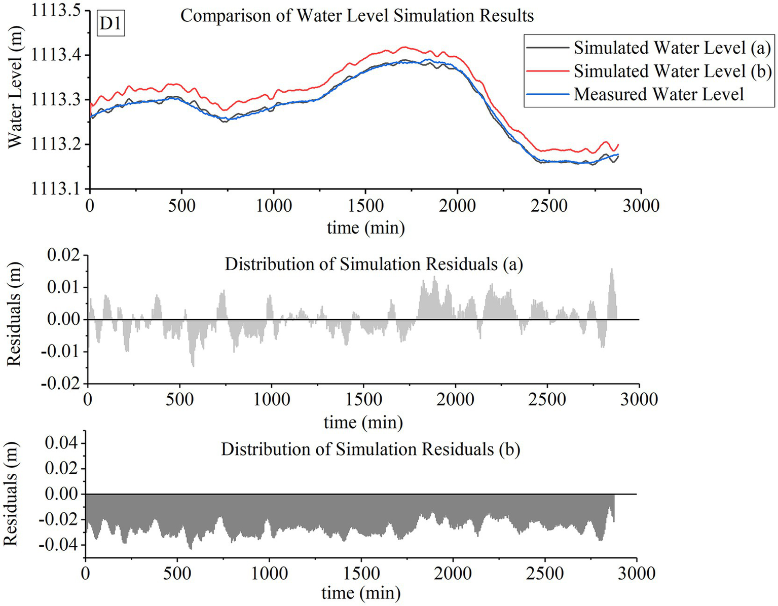
Water level simulation and residual distribution at Section D1. Simulated water level (a): Simulation using the calibrated N₀ and C0 from Table 5; Simulated water level (b): n0 = 0.0197 (Historical Usage Values), without considering seepage; Measured water level: field-measured water level data at Section D1.
Figure 6

Water level simulation and residual distribution at Section D2. Simulated water level (a): Simulation using the calibrated N₀ and C0 from Table 5; Simulated water level (b): n0 = 0.0197 (Historical Usage Values), without considering seepage; Measured water level: field-measured water level data at Section D2.
Figure 7

Water level simulation and residual distribution at Section D3. Simulated water level (a): Simulation using the calibrated N₀ and C0 from Table 5; Simulated water level (b): n0 = 0.0197 (Historical Usage Values), without considering seepage; Measured water level: field-measured water level data at Section D3.
Residual Statistical Analysis (Table 6) and Hydrological Index Comparison of Simulation Results (Table 7) are presented.
Table 6
| Parameter type | n0 | C0 | Sample size | Mean (m) | Std. Deviation (m) | Skewness |
|---|---|---|---|---|---|---|
| Calibrated parameters | 0.0179 | 1.149 | 2,880 | −0.0006 | 0.0054 | 0.0054 |
| Historical parameter | 0.0197 | 0 | 2,880 | 0.0267 | 0.0061 | 0.0061 |
Statistical parameters of fitting residuals.
Table 7
| Channel segment | n0 | C0 | MAPE | NSE | RMSE (m) | R 2 |
|---|---|---|---|---|---|---|
| S1(D1) | 0.0179 | 1.149 | 0.399 | 0.995 | 0.005 | 0.995 |
| 0.0197 | 0 | 2.446 | 0.845 | 0.027 | 0.993 | |
| S2(D2) | 0.0192 | 2.139 | 0.578 | 0.990 | 0.007 | 0.991 |
| 0.0197 | 0 | 2.759 | 0.855 | 0.027 | 0.990 | |
| S3(D3) | 0.0185 | 1.190 | 1.505 | 0.906 | 0.018 | 0.982 |
| 0.0197 | 0 | 3.087 | 0.805 | 0.033 | 0.981 |
Comparative analysis of water level simulation results.
From the water level simulation diagrams, it can be seen: simulation values and measured values at three water level measurement points using two Manning’s roughness coefficients basically coincide in the temporal water level variation trends, rising and falling phases of the curves are largely overlapping, indicating the model has good simulation capability for sustained water level rising/falling stages, corresponding to the R2 values all exceeding 0.9 in Table 7. From the residual plot, it can clearly be observed that the simulation errors using calibrated values basically fluctuate around the X-axis, while simulation parameters using the management bureau’s historical value (0.0197) mostly lie below the X-axis—meaning simulation values are generally greater than measured values, with errors significantly larger than those from simulations calibrated with measured data, consistent with MAPE results. This explains why irrigation plans formulated based on past experience frequently result in actual water levels lower than user requirements. Simulation curves under the two roughness values show slight differences from measured values at local fluctuation segments like peaks and troughs, indicating the model captures water level fluctuations well but performs poorly in simulating extreme points. From the residual plot, it can also be seen that simulation residuals at extreme points are markedly larger, with residuals using the management bureau’s historical value (0.0197) significantly exceeding those from calibrated simulations, aligning with the larger RMSE of the management bureau’s historical value (0.0197). In residual statistical analysis (Table 6), the three indicators of mean, standard deviation, and skewness all show improvements in simulations after using calibrated parameters, with the residual mean decreased by 97.64%. The minor oscillations observed in the simulation values of both cases are primarily caused by the large spatial grid scale, because the spatial step length is determined by the installation positions of monitoring equipment. From Table 2, it can be seen that the minimum spacing ds is 912 m, while the time interval is 60 s. Although the four-point implicit difference method is unconditionally stable, when the spatial step length far exceeds the time step length, it leads to insufficient discretization of the spatial solution, manifested as jumping changes in the solution—specifically, the sawtooth-like distribution near extreme points in the diagram. This situation can be improved by increasing the density of water level monitoring equipment or adopting adaptive mesh.
3.1.2 Comparison with the single-objective stepwise calibration method
To objectively evaluate the performance of the multi-objective joint calibration method (based on the NSGA-II algorithm) proposed in this study, the single-objective stepwise calibration method based on the Genetic Algorithm (GA) was selected as the benchmark for comparison. The primary reason for choosing GA as the framework for the stepwise calibration lies in its shared evolutionary algorithm framework with the NSGA-II algorithm, possessing similar optimization mechanisms (e.g., selection, crossover, mutation). This ensures consistency and fairness in the underlying logic of the comparative experiment, allowing for a more direct revelation of the intrinsic differences between the multi-objective joint optimization and single-objective stepwise optimization strategies themselves. To ensure a fair comparison, both methods utilized the Calibration dataset to calibrate the n₀ and C₀ parameters for Channel S1. The parameter settings for the stepwise calibration method (GA) were kept consistent with those for NSGA-II in Section 2.3. The core concept of this single-objective stepwise calibration method is to decompose the coupled multi-parameter calibration problem into a series of sequentially executed single-parameter optimization subproblems. The specific procedure is as follows:
Step 1: Assume the channel is without seepage (i.e., fix the seepage coefficient C₀ = 0), and calibrate Manning’s roughness coefficient n₀ individually. Use the same objective function Obj1 (see Equation 16 in Section 2.3) as used in the NSGA-II algorithm as the single objective function for calibrating n₀, aiming to find the n₀ value that achieves the best agreement between the simulated and observed water levels.
Step 2: Fix the optimal n₀ value obtained in Step 1, and calibrate the seepage parameter individually. Use the same objective function Obj2 (see Equation 17 in Section 2.3) for optimization.
The primary differences between the two methods lie in the optimization strategy (single-objective stepwise vs. multi-objective simultaneous) and the number of objective functions. The calibration results are shown in Table 8, with the solution set from the Pareto front of the NSGA-II algorithm also provided (Figure 8).
Table 8
| Calibration method | n0 | C0 | OBJ1 | OBJ2 | NSE | RMSE | R 2 |
|---|---|---|---|---|---|---|---|
| NSGA-II solution | 0.01786 | 1.1494 | 0.3990 | 1.3406 | 0.9950 | 0.0054 | 0.9940 |
| Stepwise calibration step 1 | 0.01788 | 0.0000 | 0.3989 | 100.0000 | 0.9938 | 0.0055 | 0.9941 |
| Stepwise calibration step 2 | 0.01788 | −9.9998 | 0.6017 | 0.1895 | 0.9878 | 0.0077 | 0.9939 |
Comparison of results from different calibration methods.
n₀: Manning’s roughness coefficient (unit: m−1/3/s). C0: Seepage parameter, a dimensionless empirical coefficient, calibrated using the NSGA-II algorithm. Obj1: Absolute relative error percentage between the measured and simulated water levels in the upstream section. Calculated using Equation 16. Obj2: Absolute relative error percentage between the seepage rate calculated by the water balance method and that calculated by the Davis–Wilson seepage formula. Calculated using Equation 17. NSE: Nash–Sutcliffe efficiency coefficient. Evaluates the superiority of the model compared to using only the mean value for prediction. Evaluation criterion: values closer to 1 indicate a stronger ability of the model to capture dynamic processes. Calculated using Equation 23. RMSE: Root mean square error (unit: meters). Represents the average absolute error between simulated and observed values. Evaluation criterion: values closer to 0 reflect higher simulation accuracy. Calculated using Equation 22. R2: Coefficient of determination. Measures the strength of the linear relationship between simulated and observed values, indicating trend synchronization. Evaluation criterion: values closer to 1 are more ideal. Calculated using Equation 24.
Figure 8

Pareto front solution set obtained by the NSGA-II algorithm. This Pareto front represents the solution set derived from calibrating the parameters n₀ and C₀ for Channel S1 using the NSGA-II algorithm on the Calibration dataset, respectively. The solution corresponding to the minimum value of Obj1 (i.e., the smallest water level error, represented by the leftmost point in the figure) was selected.
As shown in Table 8, during the first step of calibration, when C₀ was forced to be 0, the Manning’s roughness coefficient n₀ obtained through stepwise calibration is highly similar to one of the n₀ values from the optimal solution set derived via the NSGA-II multi-objective joint calibration. At first glance, this finding might seem to indicate the effectiveness of the single-objective method. However, it actually masks a serious “parameter equivalence” issue. Under the constraint of a fixed C₀ = 0, the optimization algorithm could only adjust n₀ to force the simulated results to match the observed data. Consequently, the resulting n₀ is not its true physical value but rather a “pseudo-optimum” that incorporates compensation for the bias introduced by neglecting seepage. It erroneously attributes the hydraulic response, which should be jointly explained by both roughness and seepage, entirely to the former.
More critically, in the second calibration step, when this potentially biased n₀ was fixed, the optimization algorithm converged to a physically unrealistic solution: C₀ = −9.99980. (When a wider parameter range was tested, C₀ became even smaller, further reducing Obj2. However, negative values are physically meaningless. Therefore, the parameter lower bound was not extended further, as the current value is sufficient to illustrate the issue.) A negative value physically implies the presence of a non-existent “water source” in the channel, which completely violates the fundamental definition of the seepage process. This absurd outcome is an inevitable product of the inherent flaw in the stepwise calibration method: it forcibly severs the intrinsic hydraulic connection between n₀ and C₀. In the subsequent calibration step, the algorithm cannot find a solution within the physically feasible domain of C₀ ≥ 0 that compensates for this error. This leads to a contradiction between mathematical optimality and physical distortion: ultimately, in pursuit of optimizing the mathematical objective function, the algorithm selects a physically impossible negative value, fitting the data by introducing fictitious water volumes. Together, these two results form a complete chain of evidence that clearly delineates the failure path of the single-objective stepwise calibration method: it first obtains a “seemingly reasonable” n₀ through parameter equivalence, and then, to maintain this flawed initial value, it has to sacrifice all physical meaning of the other parameter C₀. This demonstrates that for models with parameter interactions, pursuing stepwise, mathematically local optima ultimately leads to the collapse of overall physical significance. In sharp contrast, the NSGA-II multi-objective joint calibration method adopted in this study fundamentally avoids the above issues by simultaneously optimizing n₀ and C₀ and applying the physical constraint C₀ ≥ 0 during the search. All solutions on the Pareto front obtained by NSGA-II (Figure 8) lie within the physically feasible parameter space. Although the n₀ values of some solutions are close to those from the single-objective results, its key contribution lies in simultaneously identifying a physically credible, non-negative C₀ value.
This indicates that the joint calibration method can effectively coordinate the compensatory relationships between parameters, finding globally physically meaningful optimal or near-optimal solutions, rather than artificially distorted solutions that cause physical. For such problems, adopting a joint calibration method capable of handling parameter interactions and physical constraints is not merely an optimization choice, but a scientific necessity.
3.2 Impact of adaptive mesh refinement on simulation results
Adopting AMR technology to refine the differential grid of Test Set 1, with the refinement determination process shown in Figure 9.
Figure 9

Refinement criteria. (a) Cross-sectional spatial gradient variation; (b) Water level absolute error.
Figure 9 displays points on the temporal grid at Section D1 where the absolute error between simulated and calculated water depth exceeds the criterion (84.38% above the determination red line), and points on the spatial grid along Sections D1-D2 where the distance gradient surpasses the criterion (100% above the determination red line), exceeding the refinement threshold (30%). Refinement of the spatiotemporal grid was performed according to preset methods (Chapter 2). Table 9 provides a comparison of grids before and after refinement, while Figure 10 shows water level simulation diagrams for Section D1 before and after refinement.
Table 9
| Grid type | Criterion | Threshold | Nodes (Before) | Nodes (After) | Initial spacing | Refined spacing | Exceedance ratio |
|---|---|---|---|---|---|---|---|
| Temporal grid | Absolute error | 0.001 m | 301 | 1,501 | 300 s | 60 s | 84.38% |
| Spatial grid | Water depth gradient | 0.0001 | 2 | 31 | 912 m | 30.5 m | 100.00% |
Grid analysis before and after refinement.
Figure 10

Comparison of water level simulation results between original and refined meshes at cross-Section D1.
As shown in Figure 10, after grid refinement, the fluctuation amplitude of simulated water levels near 600–900 min and 1,200 min is significantly reduced, and the overall hydrograph aligns more closely with the measured water level curve. Post-refinement, evaluation metrics including RMSE, MAPE, R2, and NSE all show improvements: RMSE decreases from 0.0099 m to 0.0045 m, and MAPE drops from 0.6413 to 0.3804, with both reductions being approximately 50%. As RMSE is more sensitive to larger errors, its significant reduction indicates that grid refinement effectively improves points with substantial errors in the original simulation, consistent with the weakened fluctuation amplitudes in extreme-value intervals reflected in Figure 10. Meanwhile, the decline in MAPE further demonstrates that the simulation curve approximates the measured values more globally, verifying the universal applicability of the refinement method. In conclusion, AMR (Adaptive Mesh Refinement) technology exhibits clear advantages in water level simulation. Under conditions of sparse monitoring point distribution or long monitoring intervals in irrigation districts, this method can enhance simulation accuracy and offers better cost-effectiveness compared to installing additional water level observation equipment, demonstrating promising potential for broader application.
3.3 Seepage analysis
Calibration results indicate that the seepage parameters vary across different channel segments. To more intuitively visualize the spatiotemporal variation patterns of seepage rates, 3D graphs of flow hydrographs and water depth hydrographs incorporating seepage were plotted. The plotting results are shown in Figures 11, 12.
Figure 11

Flow hydrograph. Color variation represents changes in seepage rate (qs), calculated using Equation 8. For enhanced visualization, the color legend displays values scaled by a factor of 105 due to the originally small magnitude of seepage rates.
Figure 12

Water depth hydrograph. Color variation represents changes in seepage rate (qs), calculated using Equation 8. For enhanced visualization, the color legend displays values scaled by a factor of 105 due to the originally small magnitude of seepage rates.
Tables 10, 11 present the statistical indicators for seepage rate (qs) and water depth (h) respectively.
Table 10
| Channel segment | Time (min) | Sample size | Mean (m2/s) | Std. Deviation (m2/s) | Skewness |
|---|---|---|---|---|---|
| S1 | 1–1,440 | 1,440 | 4.09E−05 | 7.70E−07 | 7.70E−07 |
| 1,441–2,880 | 1,440 | 4.01E−05 | 3.05E−06 | 3.05E−06 | |
| 2,881–4,320 | 1,440 | 3.56E−05 | 1.27E−06 | 1.27E−06 | |
| S2 | 1–1,440 | 1,440 | 4.01E−05 | 7.13E−07 | 7.13E−07 |
| 1,441–2,880 | 1,440 | 3.92E−05 | 3.03E−06 | 3.03E−06 | |
| 2,881–4,320 | 1,440 | 3.48E−05 | 1.25E−06 | 1.25E−06 | |
| S3 | 1–1,440 | 1,440 | 3.48E−05 | 6.21E−07 | 6.21E−07 |
| 1,441–2,880 | 1,440 | 3.41E−05 | 2.75E−06 | 2.75E−06 | |
| 2,881–4,320 | 1,440 | 3.00E−05 | 1.13E−06 | 1.13E−06 |
Statistical metrics of qs.
Table 11
| Cross-section | Time (min) | Sample size | Mean (m) | Std. Deviation (m) | Skewness |
|---|---|---|---|---|---|
| D1 | 1–1,440 | 1,440 | 1.10 | 0.02 | 0.02 |
| 1,441–2,880 | 1,440 | 1.08 | 0.10 | 0.10 | |
| 2,881–4,320 | 1,440 | 0.94 | 0.04 | 0.04 | |
| D2 | 1–1,440 | 1,440 | 0.96 | 0.02 | 0.02 |
| 1,441–2,880 | 1,440 | 0.93 | 0.10 | 0.10 | |
| 2,881–4,320 | 1,440 | 0.79 | 0.04 | 0.04 | |
| D3 | 1–1,440 | 1,440 | 0.96 | 0.02 | 0.02 |
| 1,441–2,880 | 1,440 | 0.93 | 0.10 | 0.10 | |
| 2,881–4,320 | 1,440 | 0.79 | 0.04 | 0.04 | |
| D4 | 1–1,440 | 1,440 | 0.72 | 0.02 | 0.02 |
| 1,441–2,880 | 1,440 | 0.69 | 0.10 | 0.10 | |
| 2,881–4,320 | 1,440 | 0.54 | 0.04 | 0.04 |
Statistical metrics of water depth.
From Figures 11, 12, the spatiotemporal variation patterns of channel flow and water depth can be clearly observed, with color gradients further revealing differences in seepage volumes across distinct time periods and channel sections. Temporally, around 2,000 min, the seepage rates of Sections S1, S2, and S3 are significantly higher than those in other periods, which is closely related to the simultaneous peak water depths in all sections at this moment. Spatially, the seepage rates in Section S1 (0–912 m) and Section S2 (912–1,952 m) are markedly greater than in Section S3; notably, although Section S1 has the largest average water depth, Section S2 exhibits similarly high seepage rates due to its higher seepage coefficient (C-value). After years of operation, channels constructed with identical lining techniques show significant differences in seepage volumes among sections, attributable to three primary factors: non-uniform joint deterioration, where precast concrete panel joints exhibit spatial heterogeneity in width and sealing material aging under temperature fluctuations, stress, and frost heave effects (Liang et al., 2022; Li et al., 2023; Cao et al., 2025). Non-equivalent structural damage: where concrete slabs develop uneven cracks due to localized loads and differential foundation settlement (Aldea et al., 1999; Brush and Thomson, 2011; Han et al., 2020), and underlying geomembranes degrade at varying rates caused by chemical corrosion and UV exposure intensity discrepancies (Yi et al., 2011; Anjana et al., 2023; Lavoie et al., 2024); and differential vegetation intrusion, where plant roots growing in cracks induce root wedging effects, with penetration depths and densities diverging significantly due to microhabitat variations (Bodner et al., 2014; Hu et al., 2025). To investigate changes in seepage volumes and their proportional distribution across sections under different hydraulic conditions, subsequent analyses will divide the simulation period into three consecutive 1,440-min (one-day) intervals for detailed discussion (Table 12).
Table 12
| Canal section | Time period (min) | Avg. Depth (m) | Avg. Flow (m3/s) | Inflow (m3) | Seepage (m3) | Infil. (%) | WL Decline (%) | Infil. Decline (%) |
|---|---|---|---|---|---|---|---|---|
| S1 | 1–1,440 | 1.03 | 10.68 | 925,057 | 3,183 | 0.34 | – | – |
| 1,441–2,880 | 1.01 | 10.37 | 896,191 | 3,151 | 0.35 | 1.94 | 1.00 | |
| 2,881–4,820 | 0.86 | 8.08 | 699,400 | 2,903 | 0.42 | 14.85 | 7.87 | |
| S2 | 1–1,440 | 0.96 | 10.61 | 920,463 | 6,072 | 0.66 | – | – |
| 1,441–2,880 | 0.94 | 10.35 | 895,781 | 5,991 | 0.67 | 2.08 | 1.33 | |
| 2,881–4,820 | 0.79 | 8.04 | 697,175 | 5,520 | 0.79 | 15.96 | 7.86 | |
| S3 | 1–1,440 | 0.84 | 10.54 | 912,895 | 2,932 | 0.32 | – | – |
| 1,441–2,880 | 0.82 | 10.33 | 892,721 | 2,894 | 0.32 | 2.08 | 1.33 | |
| 2,881–4,820 | 0.67 | 8.00 | 692,340 | 2,643 | 0.38 | 18.99 | 8.67 |
Seepage analysis for different channel segments and time periods.
Average water depth and flow rate are calculated as the mean values from the start to the end of the calculation period for each segment. Total inflow refers to the cumulative water volume entering the head of the segment, while total seepage volume represents the cumulative seepage loss within the segment. Infil.: Seepage percentage (seepage volume as a percentage of total inflow); WL Decline (Water Level Decline): Percentage decrease in water level relative to the previous period; Infil. Decline (Seepage Decline): Percentage decrease in seepage volume relative to the previous period.
As shown in Table 12, within the same channel section, deeper water correlates with greater seepage volumes. This occurs because increased water depth elevates hydrostatic pressure (water head). According to Darcy’s law, seepage rates are directly governed by the hydraulic gradient (i.e., the ratio of head difference to seepage path length), where heightened water head amplifies this driving force. Additionally, greater water depth expands the wetted perimeter—the contact area between channel flow and soil—providing broader pathways for seepage Comparing water-level decline (WL column) with seepage reduction (Infil. Decline column) reveals a nonlinear relationship: water-level decline consistently exceeds seepage changes by approximately twofold. The impact of water-depth reduction on seepage also varies across sections. However, higher seepage does not imply lower effective water utilization efficiency. Contrasting Day 1 and Day 3 seepage proportions shows marked Day 3 increases (31.25, 19.70, 18.75%), while seepage volumes decrease (8.80, 9.09, 9.86%) and total inflow at the channel head declines more significantly (24.39, 24.28, 24.16%). Based on seepage percentages across segments and periods, it can be concluded that although seepage volume is higher during high-flow conditions, the channel water utilization efficiency is actually greater. Therefore, in practical operation scheduling, using short-duration high-flow releases is recommended to reduce seepage losses. The seepage volume in Canal Section S2 can reach approximately twice that of other canal sections. Depending on the ratio of seepage to total inflow (Using the maximum value 0.79 and minimum value 0.32 of this canal section), the potential irrigation benefits of seepage water savings for major crops were estimated, as summarized in the Table 13.
Table 13
| Crop type | Planting area (ha) | Gross irrigation quota (m3/ha) | Total water diversion (10,000 m3) | Seepage percentage (%) | Seepage volume (10,000 m3) | Additional irrigable area (ha) |
|---|---|---|---|---|---|---|
| Corn | 1,000.00 | 6,000.00 | 600.00 | 0.32 | 1.92 | 3.20 |
| 0.79 | 4.74 | 7.90 | ||||
| Wheat | 826.67 | 8,727.27 | 721.45 | 0.32 | 2.50 | 2.65 |
| 0.79 | 6.16 | 6.53 | ||||
| Rice | 386.67 | 17,727.27 | 685.45 | 0.32 | 2.23 | 1.24 |
| 0.79 | 5.50 | 3.05 |
Estimation of potential irrigation benefits from seepage water.
The crop planting areas and Total Water Diversion data presented in the table were derived from the three-year average (2016–2018) provided by the Fourth Management Station of the Hanyan Canal. The Gross Irrigation Quotas were calculated based on the crop-specific irrigation quotas outlined in the Water Use Quota Standard of Ningxia Hui Autonomous Region (DB64/T 971-2020) and the canal water utilization coefficient of Section (0.55).
In the Ningxia Yellow River Irrigation District, maize, wheat, and rice dominate as the top three crops by planting area (accounting for 26.41, 21.83, and 10.21% of the total cultivated area, respectively), with their irrigation almost entirely reliant on Yellow River water resources. The district rigorously enforces a “Total Volume Control and Quota Management” water resource policy, with annual water withdrawals constrained by the Yellow River Basin Water Allocation Scheme. Significant canal seepage imposes dual pressures on irrigation district operations: on one hand, water level fluctuations in canal systems caused by conveyance losses directly compromise irrigation reliability during critical crop growth stages; on the other hand, the implicit increase in Gross Irrigation Quota translates into additional economic burdens for farmers. Table 13 estimation results demonstrate that implementing anti-seepage renovations would enable this management station to expand irrigation coverage by over 3.20 hectares for maize, over 2.65 hectares for wheat, and even for water-intensive rice by over 1.24 hectares.
3.4 Sensitivity analysis
To quantify the magnitude of parameter impacts on water levels and seepage, it is essential to quantify the impact of parameter variations on water level and seepage. This study employed a global sensitivity analysis approach, using the optimal parameter solution for channel S1 calibrated by the NSGA-II algorithm as the baseline. Perturbation analysis was conducted on parameters n0 and C within ±20% of their baseline values, with each parameter discretized into five levels (−20, −10%, 0%, +10%, +20%). A total of 25 parameter combinations were generated and simulated to evaluate parameter sensitivities on RMSE and Obj2, the sensitivity heat response map results are shown in Figure 13, and the sensitivity calculation table is presented in Table 14.
Table 14
| n0 Variation coefficient | C0 Variation coefficient | Updated n0 | Updated C0 | RMSE | Percentage change in RMSE relative to baseline (100%) | OBJ2 | Percentage change in OBJ2 relative to baseline (100%) |
|---|---|---|---|---|---|---|---|
| 80% | 80% | 0.0143 | 0.9196 | 0.0500 | 825.9259 | 1.0142 | −24.3473 |
| 80% | 90% | 0.0143 | 1.0345 | 0.0501 | 827.7778 | 0.8965 | −33.1270 |
| 80% | 100% | 0.0143 | 1.1494 | 0.0502 | 829.6296 | 0.8025 | −40.1387 |
| 80% | 110% | 0.0143 | 1.2644 | 0.0502 | 829.6296 | 0.7257 | −45.8675 |
| 80% | 120% | 0.0143 | 1.3793 | 0.0503 | 831.4815 | 0.6618 | −50.6340 |
| 90% | 80% | 0.0161 | 0.9196 | 0.0260 | 381.4815 | 1.3431 | 0.1865 |
| 90% | 90% | 0.0161 | 1.0345 | 0.0261 | 383.3333 | 1.1880 | −11.3830 |
| 90% | 100% | 0.0161 | 1.1494 | 0.0261 | 383.3333 | 1.0643 | −20.6102 |
| 90% | 110% | 0.0161 | 1.2644 | 0.0262 | 385.1852 | 0.9633 | −28.1441 |
| 90% | 120% | 0.0161 | 1.3793 | 0.0263 | 387.0370 | 0.8793 | −34.4100 |
| 100% | 80% | 0.0179 | 0.9196 | 0.0054 | 0.0000 | 1.6905 | 26.1003 |
| 100% | 90% | 0.0179 | 1.0345 | 0.0054 | 0.0000 | 1.4958 | 11.5769 |
| 100% | 100% | 0.0179 | 1.1494 | 0.0054 | 0.0000 | 1.3406 | 0.0000 |
| 100% | 110% | 0.0179 | 1.2644 | 0.0055 | 1.8519 | 1.2140 | −9.4435 |
| 100% | 120% | 0.0179 | 1.3793 | 0.0055 | 1.8519 | 1.1087 | −17.2982 |
| 110% | 90% | 0.0196 | 1.0345 | 0.0261 | 383.3333 | 1.8161 | 35.4692 |
| 110% | 100% | 0.0196 | 1.1494 | 0.0260 | 381.4815 | 1.6279 | 21.4307 |
| 110% | 110% | 0.0196 | 1.2644 | 0.0260 | 381.4815 | 1.4744 | 9.9806 |
| 110% | 120% | 0.0196 | 1.3793 | 0.0259 | 379.6296 | 1.3469 | 0.4699 |
| 120% | 80% | 0.0214 | 0.9196 | 0.0522 | 866.6667 | 2.4245 | 80.8519 |
| 120% | 90% | 0.0214 | 1.0345 | 0.0521 | 864.8148 | 2.1453 | 60.0254 |
| 120% | 100% | 0.0214 | 1.1494 | 0.0520 | 862.9630 | 1.9230 | 43.4432 |
| 120% | 110% | 0.0214 | 1.2644 | 0.0519 | 861.1111 | 1.7419 | 29.9344 |
| 120% | 120% | 0.0210 | 1.3800 | 0.0520 | 859.2600 | 1.5910 | 18.7080 |
Parameter sensitivity analysis.
n0 Variation Coefficient: The calibrated roughness value for channel section S1 is taken as the baseline value. 80% indicates the baseline value multiplied by 0.8. C0 Variation Coefficient: The calibrated seepage parameter for channel section S1 is taken as the baseline value. 80% indicates the baseline value multiplied by 0.8. Updated n0/Updated C0: Represents the new n0/C0 value obtained by multiplying the baseline value by the corresponding variation percentage. RMSE: Root Mean Square Error calculated based on the measured and simulated water levels at cross-section D1 of channel S1. Represents the average absolute error between simulated and observed values. Evaluation criterion: values closer to 0 reflect higher simulation accuracy. Calculated using Equation 22. OBJ2: Absolute relative error percentage between the seepage rate calculated by the water balance method and that calculated by the Davis-Wilson seepage formula. Calculated using Equation 17. Percentage Change in RMSE/OBJ2 Relative to Baseline: The relative percentage change in RMSE and OBJ2 calculated relative to the baseline value.
In the RMSE response map, a distinct axis-parallel pattern is observed, indicating weak interaction effects between parameters n0 and C0 on RMSE. Specifically: Along the X-axis (n0 variation), when n0 deviates from its optimal value (0.01786) in either direction, RMSE increases significantly, accompanied by pronounced color gradient changes. Sensitivity calculations reveal that a ±10% variation in n0 leads to an over 300% increase in RMSE, while a ±20% variation amplifies RMSE by more than 800%, demonstrating extreme sensitivity of RMSE to n0. Along the Y-axis (C0 variation), at any fixed n0 value, the response colors remain nearly identical across different C0 values. Sensitivity data further show that a ±10% variation in C0 induces a maximum RMSE change of only ~2%, confirming insensitivity of RMSE to C0. In conclusion, RMSE is predominantly governed by n0, with C0 exerting minimal influence, consistent with the axis-parallel morphology of the response map (Figure 13).
Figure 13

Parameter sensitivity analysis: response surface heatmap. Due to the significant order-of-magnitude disparity between n0 and C0 both n0 and RMES values in the plot are scaled by 102 to enhance visual clarity.
In the Obj2 response map, oblique contour distributions suggest detectable interaction effects between n0 and C0: Along the X-axis (n0 increase), the color distribution exhibits diagonal symmetry. Sensitivity analysis indicates that progressive 10% increments in n0 uniformly elevate Obj2 values across all C0 levels, signifying a negative correlation between n0 and Obj2. Crucially, the magnitude of this increase varies depending on C0 values, further evidencing parameter interactions. Along the Y-axis (C0 increase), a similar diagonal symmetry is observed. Sensitivity analysis demonstrates that 10% increments in C0 consistently reduce Obj2 values across all n0 levels, reflecting a positive correlation between C0 and Obj2. Notably, the extent of this reduction differs with n0 values, reinforcing the presence of interaction effects. Overall, both n0 and C0 significantly influence Obj2, with their combined effects reflecting either synergistic or antagonistic relationships.
4 Discussion
Sensitivity analysis studies demonstrates that variations in n0 exert a profound impact on water levels, if irrigation schedules are developed without considering variations in n0 or based solely on past experience in water release, significant deviations between actual and planned water levels will inevitably occur, leading to situations where the water level at some headgates falls below the required value. When farmers report this to management stations, multi-gate coordinated operations are needed to adjust water levels. However, under unsteady flow conditions, such multi-gate adjustments interact with each other, making it difficult to quickly achieve the desired water level at all points. This process requires repeated adjustments, consuming time and increasing energy consumption. In this context, farmers are inclined to adopt flow-blocking or direct pumping to address their immediate needs. It should be emphasized that Ningxia, situated in the arid to semi-arid inland region of Northwest China, suffers from acute water scarcity. Water diversion quotas for branch canals of the Yellow River irrigation system strictly limit water intake, making prolonged high water level irrigation unsustainable. As a result, rotational irrigation remains the dominant operational mode. Additionally, direct offtake gates are remotely controlled, depriving farmers of autonomous flow adjustment capabilities, which further exacerbates sandbag blocking practices. Through this model, water levels at any point in the channel—especially upstream of diversion gates—can be accurately predicted, ensuring that turnout gates at all levels operate under appropriate upstream water level conditions to release the designed flow as planned, thereby avoiding unfair water distribution scenarios such as “upstream flooding and downstream drought” and guaranteeing water allocation for each farming household. Simultaneously, seepage losses are quantified and factored into the water diversion volume at the intake, preventing downstream water shortages caused by insufficient flow. This model can be further developed to establish a “digital twin” platform for the irrigation district, which can be used to test and optimize gate scheduling strategies. It allows simulation of the flow advance process under various gate opening and closing combinations in the virtual environment, thereby reducing water level fluctuations, formulating gate operation procedures that achieve the target flow most rapidly with minimal variations, improving irrigation response speed, and enabling real-time and precise irrigation district scheduling.
Field investigations during non-irrigation seasons have revealed that canals constructed during the same period exhibit significant differences in surface damage and vegetation development along different sections after years of operation. As shown in Figure 14, even within adjacent segments of the Second Eastern Main Branch Canal spanning a few 100 m, the contrast in deterioration is striking. These variations directly lead to differences in Manning’s roughness coefficient and seepage loss coefficients among canal sections. If these parameters are not specifically adjusted in the calculation of channel flow processes, significant errors in water level estimation will occur. Moreover, as canal deterioration worsens over time, seepage losses increase. If water supply plans continue to be designed based on historical operational parameters, issues such as insufficient water delivery are likely to arise, leading to missed optimal irrigation periods and reduced agricultural output. Currently, there are two major areas for optimization: first, canal renovation lacks targeted strategies and often adopts a wholesale repair model. However, given the relatively low economic returns of the agricultural sector and significant funding constraints, resource allocation must be optimized. Based on the calibration results of Manning’s roughness coefficient and seepage parameters, priority should be given to repairing canal segments with higher roughness and more severe seepage losses (As shown in Figure 14B). This approach not only shortens the construction timeline but also saves costs. The saved funds can be redirected toward the procurement of machinery, fertilizer supply, field engineering improvements, and other measures to further increase crop yield. Second, there is a need to establish a dynamic monitoring system for canal conditions. The parameter calibration method proposed in this study offers significant advantages, it only requires measured water level and flow data from a single water conveyance period to calibrate the Manning’s roughness and seepage parameters along the canal, and data collection can be synchronized with the canal flushing phase during early irrigation. Using these calibration results, more precise irrigation schedules can be developed, and targeted canal maintenance can be guided. At present, large-scale irrigation districts are already equipped with extensive water level monitoring facilities. These existing resources should be fully integrated and utilized to reduce canal seepage through accurate monitoring and maintenance, ensure desired irrigation water levels, and ultimately increase grain yield. Multiple studies have shown a positive correlation between agricultural investment and returns (Kleemann and Abdulai, 2013; Lachaud and Bravo-Ureta, 2022). Therefore, rational allocation of supporting funds for both canal maintenance and agricultural production is an essential pathway to increasing farmers’ income and ensuring food security. The core contribution of this study lies in proposing a methodological framework for simultaneously calibrating key hydraulic parameters and validating its potential to enhance the precision of irrigation scheduling and identify canal maintenance priorities. However, formulating specific quantitative water allocation schemes and accurately assessing their agricultural economic benefits requires further research. This is primarily because constructing a comprehensive decision-support system necessitates the integration of multi-year data from various departments, including detailed cropping structures, crop yields, farmer incomes, and agricultural fund allocation information. The acquisition and integration of such data remain a major challenge at this stage. Therefore, future work will focus on inter-departmental data collaboration, aiming to establish a more comprehensive database. This will enable the extension of the methodology presented in this study into a powerful tool capable of outputting quantitative optimization schemes and precisely evaluating economic benefits.
Figure 14

Photos Taken at the Irrigation District. (A) Basically intact concrete layer of the canal; (B) Severely damaged concrete layer of the canal; (C) Partially damaged concrete layer of the canal.
5 Conclusion
This study establishes a Saint-Venant equations model coupled with an empirical seepage equation, which achieves joint calibration of Manning’s roughness coefficient and seepage parameters for different types of channels based on existing monitoring facilities. By introducing adaptive mesh refinement technology, the spatiotemporal resolution and computational accuracy of channel flow simulations are significantly improved. Practical applications demonstrate that this method effectively integrates parameter identification with localized field observations, providing a quantitative basis for precise channel maintenance, thereby substantially reducing maintenance workload and costs. Quantitative sensitivity analysis results show that the root mean square error is highly sensitive to the roughness coefficient n0: a ±20% change in n0 causes the RMSE to surge by over 800%, highlighting the necessity of accurate roughness calibration in hydraulic models. In contrast, the seepage parameter C0 has a minor impact on RMSE (a ±10% change results in only about a 2% fluctuation). It is noteworthy that the interaction between the two parameters can cause the seepage evaluation indicator Obj2 to vary by up to 80.85%, indicating that both types of parameters must be considered simultaneously in channel seepage analysis. Comparative analysis further reveals that, unlike the single-objective stepwise calibration method which may yield physically unrealistic parameter values, the multi-objective joint calibration approach preserves physical consistency while maintaining computational accuracy.
Based on the above findings, it is recommended that channel managers prioritize roughness variations when developing water allocation and distribution plans. It is advisable to conduct roughness calibration using measured data during the channel flushing phase at the beginning of each irrigation season—research shows that a 10% change in roughness can lead to a prediction accuracy decline of up to 300%. For farmers growing crops such as rice that rely on stable water supply during critical periods, active inspection of significant damage sections in water supply channels should be carried out during non-irrigation seasons, with timely reporting to management authorities. Based on the dual-factor judgment method combining parameters and field observations proposed in this paper, severely damaged sections should be promptly repaired.
The applicability of this model is mainly constrained by two factors. First, the model is based on the Saint-Venant equations, so any extended application must satisfy its basic assumptions (e.g., the channel bed slope should be less than 6°). The current model is built on the basis of lined self-flow irrigation districts; if the channel contains pumping stations, they must be set as independent computational nodes, with water level monitoring points installed both upstream and downstream of the pumping stations. Second, the parameter calibration strategy adopted by the model, which aims to minimize water level errors, is primarily suitable for lined channels with low seepage rates. If applied to earth channels with high seepage losses, it is necessary to simultaneously adjust the seepage calculation formula and reevaluate the selection criteria for the Pareto front solution set to determine the optimal parameter combination under high seepage conditions. Although high-precision simulations lay a solid foundation for irrigation schedule optimization, the lack of historical gate operation data has prevented an evaluation of gate regulation efficiency. Future research should focus on integrating gate operation data to establish a coordinated optimization and dispatch system from water diversion inlets to field plots.
Statements
Data availability statement
The raw data supporting the conclusions of this article will be made available by the authors without undue reservation.
Author contributions
LL: Writing – original draft, Data curation, Conceptualization, Writing – review & editing, Methodology, Investigation. DB: Funding acquisition, Writing – review & editing, Conceptualization. YL: Writing – review & editing, Methodology. ML: Writing – original draft, Investigation. JL: Writing – original draft, Data curation. FZ: Writing – review & editing, Funding acquisition.
Funding
The author(s) declare that financial support was received for the research and/or publication of this article. This work were supported by the National Natural Science Foundation of China (Nos. 41571222, 51909208) and Shaanxi Provincial Department of Science and Technology Qinchuangyuan “Scientist+Engineer” Team Development Project (2024QCY-KXJ-100). No commercial funding was received.
Acknowledgments
We extend our gratitude to Zhou Wen and Xueli Bai for their communication and coordination with the Irrigation District Management Department, which ensured the smooth collection of experimental data.
Conflict of interest
FZ was employed by Xi'an Summit Intellilink Technologies Co., Ltd.
The remaining authors declare that the research was conducted in the absence of any commercial or financial relationships that could be construed as a potential conflict of interest.
The reviewer GL declared a shared affiliation with the authors LL, DB, YL, ML, JL to the handling editor at the time of review.
Generative AI statement
The authors declare that no Gen AI was used in the creation of this manuscript.
Any alternative text (alt text) provided alongside figures in this article has been generated by Frontiers with the support of artificial intelligence and reasonable efforts have been made to ensure accuracy, including review by the authors wherever possible. If you identify any issues, please contact us.
Publisher’s note
All claims expressed in this article are solely those of the authors and do not necessarily represent those of their affiliated organizations, or those of the publisher, the editors and the reviewers. Any product that may be evaluated in this article, or claim that may be made by its manufacturer, is not guaranteed or endorsed by the publisher.
Supplementary material
The Supplementary material for this article can be found online at: https://www.frontiersin.org/articles/10.3389/frwa.2025.1709125/full#supplementary-material
References
1
Abkar L. Kamyab S. Mehrizi A. A. Abbasi P. Vanloosdrekht M. Ghassemi A. et al . (2025). Fr om fixed points to optimum regions: AI–NSGA-II framework for high-recovery, low-energy brackish water RO. Water Res.289:124934. doi: 10.1016/j.watres.2025.124934,
2
Alam M. M. Bhutta M. N. (2004). Comparative evaluation of canal seepage investigation techniques. Agric. Water Manag.66, 65–76. doi: 10.1016/j.agwat.2003.08.002
3
Aldea C. M. Shah S. P. Karr A. (1999). Permeability of cracked concrete. Mater. Struct.32, 370–376. doi: 10.1007/Bf02479629
4
Almeida G. A. M. D. Bates P. Freer J. E. Souvignet M. (2012). Improving the stability of a simple formulation of the shallow water equations for 2-D flood modeling. Water Resour. Res.48:W05528. doi: 10.1029/2011wr011570
5
Anjana R. K. Keerthana S. Arnepalli D. N. (2023). Coupled effect of UV ageing and temperature on the diffusive transport of aqueous, vapour and gaseous phase organic contaminants through HDPE geomembrane. Geotext. Geomembr.51, 316–329. doi: 10.1016/j.geotexmem.2022.11.005
6
Aricò C. Nasello C. Tucciarelli T. (2007). A marching in space and time (mast) solver of the shallow water equations. Part II: the 2D model. Adv. Water Resour.30, 1253–1271. doi: 10.1016/j.advwatres.2006.11.004
7
Aricò C. Nasello C. Tucciarelli T. (2009). Using unsteady-state water level data to estimate channel roughness and discharge hydrograph. Adv. Water Resour.32, 1223–1240. doi: 10.1016/j.advwatres.2009.05.001
8
Ashour M. A. Aly T. E. Abu-Zaid T. S. Abdou A. A. (2023). A comparative technical study for estimating seeped water from irrigation canals in the middle Egypt (case study: El-Sont branch canal network). Ain Shams Eng. J.14:101875. doi: 10.1016/j.asej.2022.101875
9
Attari M. Hosseini S. M. (2019). A simple innovative method for calibration of Manning’s roughness coefficient in rivers using a similarity concept. J. Hydrol.575, 810–823. doi: 10.1016/j.jhydrol.2019.05.083
10
Attari M. Taherian M. Hosseini S. M. Niazmand S. B. Jeiroodi M. Mohammadian A. (2021). A simple and robust method for identifying the distribution functions of manning’s roughness coefficient along a natural river. J. Hydrol.595:125680. doi: 10.1016/j.jhydrol.2020.125680
11
Bodner G. Leitner D. Kaul H. P. (2014). Coarse and fine root plants affect pore size distributions differently. Plant Soil380, 133–151. doi: 10.1007/s11104-014-2079-8
12
Brush D. J. Thomson N. R. (2011). Fluid flow in synthetic rough-walled fractures: Navier-stokes, stokes, and local cubic law simulations. Water Resour. Res.39, 1037–1041. doi: 10.1029/2002wr001346
13
Cant R. S. Ahmed U. Fang J. Chakarborty N. Nivarti G. Moulinec C. et al . (2022). An unstructured adaptive mesh refinement approach for computational fluid dynamics of reacting flows. J. Comput. Phys.468:111480. doi: 10.1016/j.jcp.2022.111480
14
Cao L.-F. Li Y.-C. Huang B. (2025). Leakage of composite cutoff walls through geomembrane joint defects. Geotext. Geomembr.53, 1063–1075. doi: 10.1016/j.geotexmem.2025.04.002
15
Chen F. Cui N. Jiang S. Wang Z. Li H. Lv M. et al . (2023). Multi-objective deficit drip irrigation optimization of citrus yield, fruit quality and water use efficiency using NSGA-II in seasonal arid area of Southwest China. Agric. Water Manag.287:108440. doi: 10.1016/j.agwat.2023.108440
16
Deng M. Li Z. Wang W. Zhang J. Xiang K. Wang Y. (2025). A multi-objective optimization framework for check dam siting integrating GIS, a hydrological–hydrodynamic coupling model, and NSGA-II. J. Hydrol.134557:134557. doi: 10.1016/j.jhydrol.2025.134557,
17
Errico A. Pasquino V. Maxwald M. Chirico G. B. Solari L. Preti F. (2018). The effect of flexible vegetation on flow in drainage channels: estimation of roughness coefficients at the real scale. Ecol. Eng.120, 411–421. doi: 10.1016/j.ecoleng.2018.06.018
18
Fan Y. Chen H. Gao Z. Fan Y. Chang X. Yang M. et al . (2023). Water distribution and scheduling model of an irrigation canal system. Comput. Electron. Agric.209:107866. doi: 10.1016/j.compag.2023.107866
19
Feldmann D. Laux P. Heckl A. Schindler M. Kunstmann H. (2023). Near surface roughness estimation: a parameterization derived from artificial rainfall experiments and two-dimensional hydrodynamic modelling for multiple vegetation coverages. J. Hydrol.617:128786. doi: 10.1016/j.jhydrol.2022.128786
20
Ghobadian R. Fathi-Moghadam M. (2014). Estimation of seepage losses in ephemeral network and branching streams. J. Hydrol. Eng.19, 299–307. doi: 10.1061/(Asce)He.1943-5584.0000788
21
Han X. Wang X. Zhu Y. Huang J. (2021). A fully coupled three-dimensional numerical model for estimating canal seepage with cracks and holes in canal lining damage. J. Hydrol.597:126094. doi: 10.1016/j.jhydrol.2021.126094
22
Han X. Wang X. Zhu Y. Huang J. Fu F. J. W. (2020). An experimental study on concrete and geomembrane lining effects on canal seepage in arid agricultural areas. Water12:2343. doi: 10.3390/w12092343
23
Han X. Wang X. Zhu Y. Wu J. Huang J. (2022). Effects of canal damage characteristics on canal seepage based on a three-dimensional numerical model. J. Hydrol.605:127295. doi: 10.1016/j.jhydrol.2021.127295
24
He S. Ma Z. Qin X. You J. Wen T. Gao Y. et al . (2025). Deriving hybrid reservoir group operation rules for droughts using integrated NSGA-II framework and operation models. J. Hydrol.661:133696. doi: 10.1016/j.jhydrol.2025.133696
25
Hu J. Ren Y. Tang M. Zhang Z. Yang K. Zhen Q. et al . (2025). Effects of vegetation restoration on infiltration patterns and preferential flow in semi-arid areas with shallowly buried soft bedrock (Pisha sandstone) in China. J. Hydrol.661:133546. doi: 10.1016/j.jhydrol.2025.133546
26
Khaeez S. Hashemy Shahdany S. M. (2021). Non-structural modification of agricultural water distribution systems in large scale irrigation districts. Comput. Electron. Agric.184:106102. doi: 10.1016/j.compag.2021.106102
27
Kleemann L. Abdulai A. (2013). Organic certification, agro-ecological practices and return on investment: evidence from pineapple producers in Ghana. Ecol. Econ.93, 330–341. doi: 10.1016/j.ecolecon.2013.06.017
28
Kong F. Liu Z. Lin C. Wang Z. Wang W. Yao S. et al . (2025). Experimental study and parameter optimization of desiccant wheel-assisted atmospheric water harvesting system based on NSGA-II. Energy Convers. Manag.339:119943. doi: 10.1016/j.enconman.2025.119943
29
Krityakierne T. Sinpayak P. Khiripet N. (2025). Gis spatial optimization for agricultural crop allocation using NSGA-II. Inf. Process. Agric.12, 139–150. doi: 10.1016/j.inpa.2024.04.005
30
Lachaud M. A. Bravo-Ureta B. E. (2022). A Bayesian statistical analysis of return to agricultural R&D investment in Latin America: implications for food security. Technol. Soc.70:102054. doi: 10.1016/j.techsoc.2022.102054
31
Lavoie F. L. Kobelnik M. Valentin C. A. Lopes M. D. L. Silva J. L. D. Palmeira E. M. (2024). Study of heat and UV radiation exposures on HDPE geomembranes. Results Mater.22:100552. doi: 10.1016/j.rinma.2024.100552
32
Li Y. Chai J. Li Y. Wang R. Qin Y. Cao Z. (2023). Experimental investigation of the interfacial bonding properties between polyurethane mortar and concrete under different influencing factors. Constr. Build. Mater.408:133800. doi: 10.1016/j.conbuildmat.2023.133800
33
Li Z. Mu T. Li X. Li P. Feng J. Xu H. et al . (2025). Physics-informed neural network for hydraulic prediction in open-channel water transfer projects with sparse monitoring data. Water Res.287:124507. doi: 10.1016/j.watres.2025.124507,
34
Liang Y. Zhang F. Jing M. He P. J. (2022). Research on mechanical model of canal lining plates under the effect of frost heaving force. Adv. Civ. Eng.2022. doi: 10.1155/2022/8762382
35
Lund A. A. R. Gates T. K. Scalia J. (2023). Characterization and control of irrigation canal seepage losses: a review and perspective focused on field data. Agric. Water Manag.289:108516. doi: 10.1016/j.agwat.2023.108516
36
Ma Q. Yang Y. Sheng Z. Han S. Yang Y. Moiwo J. P. (2022). Hydro-economic model framework for achieving groundwater, food, and economy trade-offs by optimizing crop patterns. Water Res.226:119199. doi: 10.1016/j.watres.2022.119199,
37
Offermans N. Massaro D. Peplinski A. Schlatter P. (2023). Error-driven adaptive mesh refinement for unsteady turbulent flows in spectral-element simulations. Comput. Fluids251:105736. doi: 10.1016/j.compfluid.2022.105736
38
Ryu J. Bae I. Haque L. F. S. Jang E.-K. Ji U. (2025). Assessing water surface profile simulations with bulk flow resistance and composite roughness methods in partially vegetated channels. KSCE J. Civ. Eng.100456:100456. doi: 10.1016/j.kscej.2025.100456,
39
Wang Z. Cao C. Yu Q. Shen J. Han M. Xia W. et al . (2025). Uneven frost heave deformation in water conveyance channels in cold-arid regions: experimental evidence and thermo-hydro-mechanical coupling analysis. J. Rock Mech. Geotech. Eng.17, 7107–7126. doi: 10.1016/j.jrmge.2024.12.019
40
Xu C. Zhou X. Ren H. Sutulo S. Guedes Soares C. (2024). Real-time calculation of ship to ship hydrodynamic interaction in shallow waters with adaptive mesh refinement. Ocean Eng.295:116943. doi: 10.1016/j.oceaneng.2024.116943
41
Yi S. T. Hyun T. Y. Kim J. K. (2011). The effects of hydraulic pressure and crack width on water permeability of penetration crack-induced concrete. Constr. Build. Mater.25, 2576–2583. doi: 10.1016/j.conbuildmat.2010.11.107
42
Zevallos J. Chávarri-Velarde E. Gutierrez R. R. Lavado-Casimiro W. (2025). Bayesian calibration of a 2D hydraulic model using a convolutional neural network emulator. Environ. Model. Softw.193:106621. doi: 10.1016/j.envsoft.2025.106621
43
Zhou L. Yan P. Han Z. Zhang Z. Lei X. Wang H. (2023). Roughness inversion of water transfer channels from a data-driven perspective. Water15:17. doi: 10.3390/w15152822
44
Zhu Y. Zhao S. Zhou Y. Liang H. Bian X. (2025). An unstructured adaptive mesh refinement for steady flows based on physics-informed neural networks. J. Comput. Phys.540:114283. doi: 10.1016/j.jcp.2025.114283
Summary
Keywords
irrigation district, digital agriculture, sustainable agriculture, hydraulic model, precision irrigation
Citation
Li L, Bai D, Li Y, Li M, Lei J and Zhen F (2025) Joint calibration of Manning’s roughness and seepage in canals using NSGA-II for precision hydrodynamic modeling. Front. Water 7:1709125. doi: 10.3389/frwa.2025.1709125
Received
24 September 2025
Revised
19 November 2025
Accepted
21 November 2025
Published
12 December 2025
Volume
7 - 2025
Edited by
Reza Kerachian, University of Tehran, Iran
Reviewed by
Ge Li, Xi'an University of Technology, China
Hadi Rezaei Rad, Nuclear Science and Technology Research Institute (NSTRI), Iran
Fatemeh Soroush, Vali-e-Asr University of Rafsanjan, Iran
Updates
Copyright
© 2025 Li, Bai, Li, Li, Lei and Zhen.
This is an open-access article distributed under the terms of the Creative Commons Attribution License (CC BY). The use, distribution or reproduction in other forums is permitted, provided the original author(s) and the copyright owner(s) are credited and that the original publication in this journal is cited, in accordance with accepted academic practice. No use, distribution or reproduction is permitted which does not comply with these terms.
*Correspondence: Dan Bai, baidan@xaut.edu.cn
Disclaimer
All claims expressed in this article are solely those of the authors and do not necessarily represent those of their affiliated organizations, or those of the publisher, the editors and the reviewers. Any product that may be evaluated in this article or claim that may be made by its manufacturer is not guaranteed or endorsed by the publisher.