Robust Feedback Control for Discrete-Time Systems Based on Iterative LMIs with Polytopic Uncertainty Representations Subject to Stochastic Noise

1 Introduction

The research field of linear control theory is well investigated and facilitates generalized and efficient methods to design linear controllers for linear systems. For example, LMI methods have been established for the robust controller design and used to prove asymptotic stability of the closed loop simultaneously.

However, as almost all real systems are nonlinear, these methods do not ensure stability for real-world applications. To make use of the efficiency of linear methods nonetheless, these nonlinearities, if bounded, can be expressed as polytopic domains just like (time-varying) uncertainties. For this purpose, the nonlinear model can be transformed into a quasi-linear form, whereby the bounded nonlinearities can be evaluated using interval arithmetic (Rauh and Romig, 2021; Rauh et al., 2021). For these systems, a convex LMI approach is just as applicable as for pure parameter uncertainty. In such cases, a polytopic representation of the uncertainties is required, which is bounded by the element-wise defined realizations. Hence, by taking the uncertainties into account in the controller design, stability of the nonlinear closed loop can be guaranteed.

Additionally, process and measurement noise appear in all real systems. These noise processes can lead to oscillatiosn in the control loop or to excessively large control amplitudes and therefore should be suppressed. This can be achieved for example by an observer-based state feedback structure. However, with the plant being nonlinear, the separation principle is not valid. Therefore, the controller and the observer must be designed simultaneously to ensure stability (Ibrir, 2008; Rauh et al., 2021). The problem of simultaneously designing discrete-time observers and controllers for uncertain systems is also considered, for example, in Peaucelle and Ebihara (2014); Zemouche et al. (2016). These works also make use of a Lyapunov-based LMI approach. However, noise reduction is not discussed. In Ibrir (2008) as well as in Kheloufi et al. (2014), observed-based controllers are designed for Lipschitz nonlinear systems under H_∞ conditions. Another control design method for nonlinear systems with a noise and disturbance compensation based on LMI techniques is shown in Furtat (2018) such as in Yucelen et al. (2010) as a robust output feedback control on the basis of active noise control. In De Oliveira et al. (2002) and Sadabadi and Karimi (2013), LMI methods are used to design dynamic and static output feedback controllers for discrete-time systems subject to H_∞ and H₂ conditions. A further Lyapunov-based LMI approach with polytopic domains is shown for switched linear discrete-time systems in Phat and Ratchagit (2011); Ratchagit and Phat (2011) and Yotha and Mukdasai (2013), where delays are represented with intervals.

In the continuous-time case, a desensitization to stochastic noise is already investigated, for example, in Rauh et al. (2014); Rauh et al. (2018); Rauh and Romig (2021); Rauh et al. (2021). It is especially pointed out how standard low-pass-filtering can lead to oscillation for stochastic systems with an observer-based or a filter-based controller design. To counter such oscillations, an optimization task is presented, which minimizes the area for which stability cannot be proven. This optimization task is solved by a numerical LMI-based method, which can be applied for a filter or observer design with a previously designed controller. In Rauh and Romig (2021), this work is extended by considering bounded parameter uncertainty and a simultaneous controller and linear filter design. Thereby, the entire closed loop can be designed as insensitive as possible against parameter uncertainty and stochastic noise. The same optimization task is used in Rauh et al. (2021) to design an observer-based output feedback or an observer-based state feedback controller. The reason for the separation of those articles is the fact that the design criteria are not fully identical for the requirements of different control structures.

However, a discrete-time controller is required for the implementation on a microcomputer. Therefore, the continuous-time system is sampled, which leads to a discrete-time representation of the plant. To deal with these systems, methods are required that consider the discretization in the design.

This paper deals with a discrete-time LMI approach while simultaneously optimizing the observer and controller gains. Additionally, the article solves the issue that different closed loops lead to different design criteria. Hereby, a joint optimization algorithm is developed, which can be applied to a myriad of closed loop structures. For that purpose, we address the structured linear control (SLC) problem in which the dynamic controller is described as a structured state feedback approach in an augmented system model. In this paper, the procedure is shown explicitly for the design of an observer-based state feedback control. Through a superposed iteration rule, the LMI design parameters are the same as the parameters to be implemented. The direct discrete-time design allows the offline-computed control parameters to be transferred directly to the microcomputer. Due to the consideration of noisy output equations, leading to a direct disturbance feedthrough term, a classical H₂ optimization cannot be applied. Moreover, the presence of polytopic domains invalidates the parameterization of classical LQG approaches. To overcome both limitations and to obtain a discrete-time noise-insensitive controller, we forecast the influence of noise on the closed loop behavior by discrete-time increments of the Lyapunov function candidate. This leads to the discrete-time counterpart of the Itô differential operator from Rauh and Romig (2021); Rauh et al. (2021). Thereby, the uncertainty domains are quantified and subsequently minimized.

By solving the proposed optimization task, a noise-insensitive controller is obtained. With its help, the actual state trajectories converge as closely as possible to the desired operating point. In addition, this framework has the capability to robustly prescribe the desired system dynamics in terms of a discrete-time ${\mathcal{D}}_{\text{R}}$-region concept, see Dehnert (2020). This approach allows for specifying admissible eigenvalue domains of the closed loop to adjust the control performance. In the proposed approach, the simultaneous optimization of the observer dynamics and of the controller gains results in bilinear matrix inequalities (BMIs). To find a solution of these BMIs, an iterative algorithm is designed, in which LMIs are solved in each iteration stage. Such iterative LMI algorithms for discrete-time systems have already been published for example in Dehnert et al. (2015); Grunert et al. (2019); Dehnert (2020); Dehnert et al. (2020); Lerch et al. (2021b); Lerch et al. (2021a) in various other contexts. The use of LMIs provides an efficient and numerically stable design method and allows to account for bounded parameter uncertainty or nonlinearities by means of a convex combination of extremal system realizations. In this approach, closed-loop stability is ensured by using a quadratic Lyapunov function candidate and the objective is to design linear controllers and observers with constant gains in order to reduce the online implementation effort.

This paper is structured as follows. Within a problem description in Section 2, the observer-based output feedback controller is introduced. This is followed in Section 3 by the necessary basics of the work, which consist of the description of polytopic domains, robust Lyapunov stability and robust ${\mathcal{D}}_{\text{R}}$ regions. Subsequently, the main result is presented in Section 4. Here, also the convergence of the superimposed iteration rule is studied, as well as a derivation of the discrete version of the Itô differential operator used for the reduction of the influence of noise. The efficiency of the proposed approach is demonstrated in Section 5 for a point-to-point control of an overhead traveling crane with bounded nonlinearities. Stochastic noise accounts for non-modeled external disturbances in the state equations and for perturbations in the available measurements. Finally, conclusions and an outlook on future work are provided in Section 6.

2 Problem Statement

2.1 Desensitization of the Closed Loop to Stochastic Noise in the Continuous-Time Case

Consider the continuous-time linear noisy system

$\begin{array}{cc}\hfill \dot{x}& =A_{c}x+B_c\left(u+G_{cu}{w}_u\right)+G_p{w}_p\hfill \\ \hfill y& =Cx+G_y{w}_y\hfill \end{array}(1)$

with the state vector $x\in {\mathbb{R}}^n$; the input vector $u\in {\mathbb{R}}^m$; the output vector $y\in {\mathbb{R}}^p$; the system matrix A_c; the input matrix B_c and the output matrix C; the stochastically independent standard normally distributed Brownian motions of actuator noise, process noise and sensor noise $w_u\in {\mathbb{R}}^{m_u}$, $w_p\in {\mathbb{R}}^{m_p}$ and $w_y\in {\mathbb{R}}^{m_y}$, respectively; the disturbance input matrices G_cu, G_p and G_y contain the corresponding standard deviations.

To prove the stability of system (Eq. 1), the time derivative L(V) in the form of its stochastic interpretation of the Lyapunov function candidate $V(x)=\frac{1}{2}{x}^{\mathrm{T}}Px$ has to be negative definite. Due to the stochastic noise, this leads to the Itô differential operator (Kushner, 1967), which can be expressed by

$L\left(V\right)=\frac{1}{2}\left(x^{\mathrm{T}}\left({\mathcal{A}}^{\mathrm{T}}P+P\mathcal{A}\right)x+\mathrm{t}\mathrm{r}\mathrm{a}\mathrm{c}\mathrm{e}\left\{{\mathcal{G}}^{\mathrm{T}}P\mathcal{G}\right\}\right)(2)$

with the augmented system matrices $\mathcal{A}$ and $\mathcal{G}$ of the considered closed loop (Rauh et al., 2014; Rauh et al., 2018). However, due to the noise, it is possible that L(V) is positive definite in the neighborhood of x = 0. This non-provable stability region is the interior of an ellipsoid and its boundary can be specified by L(V) = 0. The Itô differential operator (Eq. 2) has been used in various contexts, also for uncertain systems in Rauh and Romig (2021) and Rauh et al. (2021). A derivation can be found in Senkel et al. (2016). The objective of the proposed study is to employ this operator analogously for discrete-time control systems to design observer-based state feedback controllers.

2.2 Desensitization of the Closed Loop to Stochastic Noise in the Discrete-Time Case

In the following, we consider multivariable nonlinear discrete-time systems subject to noise represented by the quasi-linear form

$\begin{array}{cc}\hfill x\left[k+1\right]& =A\left(x\left[k\right]\right)x\left[k\right]+B\left(x\left[k\right]\right)\left(u\left[k\right]+G_u{w}_u\left[k\right]\right)+G_p{w}_p\left[k\right]\hfill \\ \hfill y\left[k\right]& =Cx\left[k\right]+G_y{w}_y\left[k\right]\hfill \end{array}(3)$

with the same nomenclature as in Eq. 1. The nonlinearity of the system is assumed only in the state equation, i.e., the matrices $A\left(x\left[k\right]\right)$ and $B\left(x\left[k\right]\right)$ are dependent on the states $x\left[k\right]$, whereas the measurement equation is linear. For more detailed information on quasi-linear systems, see Coetsee (1994). In general, the influence of noise is reduced by a suitable filter. Since an observer also has a filtering characteristic, the aim of this paper is to present a method to design a linear observer-based state feedback controller for nonlinear systems of the form (Eq. 3). Due to the nonlinearities, the separation theorem is no longer valid, which means that controller and observer can influence each other’s stability and must be designed simultaneously (Rauh et al., 2021). Therefore, the closed loop system of the observer-based state feedback is considered in the next step. The discrete-time state-space representation of a linear time-invariant full state observer is given by

$\widehat{x}\left[k+1\right]=A_{\mathrm{n}\mathrm{o}\mathrm{m}}\widehat{x}\left[k\right]+B_{\text{nom}}u\left[k\right]+H\left(y\left[k\right]-C\widehat{x}\left[k\right]\right)(4)$

with the observer gain $H\in {\mathbb{R}}^{n\times p}$ and the nominal matrices A_nom and B_nom, which are determined by a suitable linearization or by the evaluation of the quasi-linear system matrix for a representative operating point. With that, all estimated states $\widehat{x}$ can be fed back by the control law

$u\left[k\right]=-K\widehat{x}\left[k\right]+Sr\left[k\right]$

with the controller gain $K\in {\mathbb{R}}^{m\times n}$, the reference variable $r\left[k\right]\in {\mathbb{R}}^p$ and the feedforward gain $S\in {\mathbb{R}}^{m\times p}$. Without loss of generality, we assume that $r\left[k\right]=0$. By formulating (Eq. 4) as an error model with

$e\left[k\right]=x\left[k\right]-\widehat{x}\left[k\right],$

the augmented closed loop system

$\begin{array}{ll}\hfill z\left[k+1\right]& =\left(\begin{array}{cc}A\left(x\left[k\right]\right)-B\left(x\left[k\right]\right)K\hfill & B\left(x\left[k\right]\right)K\hfill \\ \hfill A\left(x\left[k\right]\right)-A_{\mathrm{n}\mathrm{o}\mathrm{m}}-\left(B\left(x\left[k\right]\right)-B_{\mathrm{n}\mathrm{o}\mathrm{m}}\right)K\hfill & A_{\mathrm{n}\mathrm{o}\mathrm{m}}-HC-\left(B_{\mathrm{n}\mathrm{o}\mathrm{m}}-B\left(x\left[k\right]\right)\right)K\hfill \end{array}\right)z\left[k\right]\hfill \\ \hfill & +\left(\begin{array}{ccc}\hfill B\left(x\left[k\right]\right)G_u\hfill & \hfill G_p\hfill & \hfill 0_{n\times m_y}\hfill \\ \hfill B\left(x\left[k\right]\right)G_u\hfill & \hfill G_p\hfill & \hfill -H{G}_y\hfill \end{array}\right)w\left[k\right]≕\mathcal{A}\left(x\left[k\right]\right)z\left[k\right]+\mathcal{G}\left(x\left[k\right]\right)w\left[k\right]\hfill \end{array}(5)$

can be derived with

$z\left[k\right]={\left(\begin{array}{cc}\hfill x^{\mathrm{T}}\left[k\right]\hfill & \hfill e^{\mathrm{T}}\left[k\right]\hfill \end{array}\right)}^{\mathrm{T}}\mathrm{a}\mathrm{n}\mathrm{d}w\left[k\right]={\left(\begin{array}{ccc}\hfill w_u^{\mathrm{T}}\left[k\right]\hfill & \hfill w_p^{\mathrm{T}}\left[k\right]\hfill & \hfill w_y^{\mathrm{T}}\left[k\right]\hfill \end{array}\right)}^{\mathrm{T}}.$

The closed loop structure is visualized in Figure 1.

FIGURE 1

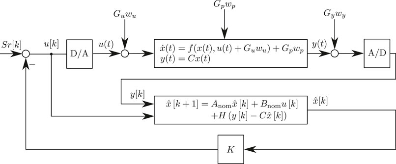
FIGURE 1. Block diagram of the discrete-time observer-based state feedback control system.

1. Note that, due to the improved implementability for real-world applications, a linear control concept is shown in this paper. In Section 5.2, we elaborate a comparison with a standard LQG approach with an identical control strukture as shown in Figure 1. Both controllers (LMI-based optimization and classical LQG) should have the same control structure so that the implementation effort is identical. This yields enhanced comparability. The most important point here is that real-time implementability is provided even if the computing capacity is limited. Since only matrix-vector products have to be computed in the subsequent operation of the observer-based controls, the implementation effort is minimal in both cases.The aim of this paper is to determine the constant gain matrices K and H (which will be decision variables in the LMI approach) in such a way that noise is suppressed effectively. Thereby, the influence of noise on the controlled system decreases and the controller is able to follow the reference variables as accurately as possible with reduced oscillations. Furthermore, a stability proof for the closed loop system will be given, such that controller and observer stabilize the nonlinear system in a predefined operating range.

3 Fundamentals for the Controller Design

3.1 Modeling with Polytopic Domains

Consider the nonlinear discrete-time system (Eq. 3). If the states $x\left[k\right]={\left(x_1\left[k\right],\dots ,x_n\left[k\right]\right)}^{\mathrm{T}}$ of the system (Eq. 3) are constrained by known limits, such that $x_i\in \left[{\underline{x}}_i,{\bar{x}}_i\right],i=1,\dots ,n$, it is possible to interpret all matrix entries as bounded by a polytopic domain. For this purpose, new independent parameters can be introduced for all matrix entries in which dissimilar nonlinearities appear. The procedure is shown in detail in Section 5.1. The matrices $A\left(x\left[k\right]\right)$ and $B\left(x\left[k\right]\right)$ belong to the convex combination

$\left[A\left(x\left[k\right]\right),B\left(x\left[k\right]\right)\right]\in \left\{\left[A\left(\zeta \right),B\left(\zeta \right)\right]=\sum _{v=1}^{n_v}{\zeta }_v\cdot \left[A_v,B_v\right];\sum _{v=1}^{n_v}{\zeta }_v=1;{\zeta }_v\ge 0\right\}(6)$

of the extremal vertex matrices A_v and B_v, where n_v denotes the number of independent extremal realizations for the union of all matrices included in Eq. 6. With this representation, it is possible to consider constant or time-varying uncertain parameters with known bounds (Scherer and Weiland, 1994; Boyd et al., 1997). Measurement tolerances for specific system parameters, fabrication tolerances or system nonlinearities can be accounted for by this uncertainty model. Furthermore, these uncertain parameters can be used to describe unidentifiable parts of the system dynamics or to cover different or even faulty system variants. In this work, the parameters ζ_v are functions of the states $x\left[k\right]$, thus they are time-varying. The closed loop (Eq. 5) with the matrices $\mathcal{A}\left(x\left[k\right]\right)$ and $\mathcal{G}\left(x\left[k\right]\right)$ can then be expressed by

$\left[\mathcal{A}\left(x\left[k\right]\right),\mathcal{G}\left(x\left[k\right]\right)\right]\in \left\{\left[\mathcal{A}\left(\zeta \right),\mathcal{G}\left(\zeta \right)\right]=\sum _{v=1}^{n_v}{\zeta }_v\cdot \left[{\mathcal{A}}_v,{\mathcal{G}}_v\right];\sum _{v=1}^{n_v}{\zeta }_v=1;{\zeta }_v\ge 0\right\}(7)$

with the n_v extremal vertex matrices ${\mathcal{A}}_v$ and ${\mathcal{G}}_v$. The linear variables ζ_v depends nonlinearly upon the state variables. Therefore, the expression (Eq. 7) is restrictive and some of the vertex matrices have unphysical properties. This overapproximation, caused by the convex enclosure of the nonlinearities, is typically not unique and can vary depending on the chosen vertex matrices.

3.2 Quadratic Lyapunov Stability

To guarantee robust stability of the autonomous closed loop (Eq. 5) with $w\left[k\right]=0$ for the bounded set (Eq. 7), a quadratic Lyapunov function candidate is given by

$V\left(z\left[k\right]\right)=\frac{1}{2}z{\left[k\right]}^{\mathrm{T}}Pz\left[k\right]$

with P = P^T ≻ 0 as a free decision variable. The uncertain closed loop (Eq. 5) with the polytopic domain (Eq. 7) is robustly (quadratically) stable if the Lyapunov conditions

${\mathcal{A}}_v^{\mathrm{T}}P{\mathcal{A}}_v-P\prec 0,\mathrm{w}\mathrm{i}\mathrm{t}\mathrm{h}v=1,\dots ,n_v(8)$

are fulfilled (Scherer and Weiland, 1994). Therefore, it is sufficient that the increment ΔV = V(z[k + 1]) − V(z[k]) is negative definite. Remind that ${\mathcal{A}}_v$ depends on the control and observer parameters, which are also decision variables. Therefore, (Eq. 8) are nonlinear matrix inequalities, hence, solving for P and ${\mathcal{A}}_v$ simultaneously by an LMI solver is not directly possible. For this reason, an overlaid iterative LMI method is presented in Section 4 that ensures stability of the closed loop.

3.3 Robust ${\mathcal{D}}_{\text{R}}$ Regions

Due to the robust design procedure, a direct pole placement is not possible. This issue is resolved by robust ${\mathcal{D}}_{\text{R}}$ regions, which are subsets of the unit circle. By a pole region placement for all extreme matrices of the convex hull (Eq. 7) within the domain ${\mathcal{D}}_{\text{R}}$, stability is proven and certain closed loop characteristics can be realized. For example, a numerically efficient region for a high damping characteristic is sketched in Figure 2. This corresponds to the matrix inequalities

${\left({\mathcal{A}}_v-\alpha I\right)}^{\mathrm{T}}P\left({\mathcal{A}}_v-\alpha I\right)-r^{2}P\prec 0,\mathrm{w}\mathrm{i}\mathrm{t}\mathrm{h}v=1,\dots ,n_v,(9)$

where |α + r|⩽1 with 0 < r < 1 and −1 < α < 1. If (Eq. 9) are satisfied, the system (Eq. 5) is robustly stable and all eigenvalues of the extremal realizations (Eq. 7) are located within the circular sub-region of the unit circle (Dehnert, 2020; Rauh, 2017; Wahab, 1994).

FIGURE 2

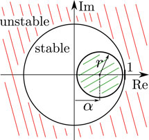
FIGURE 2. Robust circular ${\mathcal{D}}_{\text{R}}$ region.

This transformation maps the unit circle with radius r = 1 and center at the origin α = 0 onto a circle of radius r < 1 and center at α on the real axis in the complex plane. The radius r is also called exponential decay rate and α is an eigenvalue shift operator. By minimizing this ${\mathcal{D}}_{\text{R}}$ region and moving towards the origin, the convergence rate of the closed loop can be maximized. Further, with solely positive eigenvalues with a small imaginary part, oscillations are minimized, which corresponds to a larger damping.

4 Main Results

4.1 Iterative Offline Observer Based Controller Design with Robust ${\mathcal{D}}_{\text{R}}$ Region Criteria

First we assume that w[k] = 0 is true, then the stability of the deterministic, noise-free part of the augmented system (Eq. 5) can be proven by the conditions (Eq. 9), which are equivalent to

$\left(\begin{array}{cc}\hfill P^{-1}\hfill & \hfill \left({\mathcal{A}}_v-\alpha I\right)\hfill \\ \hfill {\left({\mathcal{A}}_v-\alpha I\right)}^{\mathrm{T}}\hfill & \hfill r^{2}P\hfill \end{array}\right)\succ 0,v=1,\dots ,n_v(10)$

after applying the Schur complement. To linearize the inverse of the matrix P, we consider the constant matrix $\widehat{P}={\widehat{P}}^{\mathrm{T}}\succ 0$ as an approximation of P. Then, P⁻¹ can be linearized by

$P^{-1}\succcurlyeq 2{\widehat{P}}^{-1}-{\widehat{P}}^{-1}P{\widehat{P}}^{-1}≕L(11)$

[Dehnert, 2020]. Due to P⁻¹ ≽ L, the nonlinear matrix inequalities (Eq. 10) are always satisfied if the LMIs

$\left(\begin{array}{cc}\hfill L\hfill & \hfill \left({\mathcal{A}}_v-\alpha I\right)\hfill \\ \hfill {\left({\mathcal{A}}_v-\alpha I\right)}^{\mathrm{T}}\hfill & \hfill r^{2}P\hfill \end{array}\right)\succ 0,v=1,\dots ,n_v(12)$

are fulfilled. The proof of inequality (Eq. 11) can be found in Dehnert et al. (2015) or Dehnert (2020). Note that the inequality (Eq. 11) becomes an equality if $P=\widehat{P}$ holds. In the developed algorithm, the matrix $\widehat{P}$ is inherited from the last iteration by the update rule

${\widehat{P}}_l=P_{l-1},(13)$

where l is the current iteration. This leads to a successively closer approximation of P. The initialization of the update rule (Eq. 13) can be done with ${\widehat{P}}_0=I$, see Section 4.2. By this update rule, the non-convex problem caused by the matrix inequalities (Eq. 10) can be simplified into a sequence of convex subproblems.

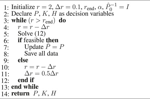
In a first step, the feasibility problem is formulated in the form of our method in Algorithm 1. This procedure ensures that a valid solution is determined, however, yet without any optimization. This solution then represents the starting point for further optimizations. By using Algorithm 1, the nonlinear problem is reduced to an iterative LMI algorithm. Algorithm 1 is essential because the initialization of ${\widehat{P}}_0^{-1}=I$ may be far off the real inverse of P, which can lead to infeasibility. To address this problem, r > 1 is required in the first iteration. Subsequently, r is decreased successively to obtain a stable solution. In each iteration step l, the constant matrix $\widehat{P}$ is only updated if the LMI problem is feasible. Otherwise, the latest feasible solution is restored and the step size Δr is halved to obtain a feasible solution in the next iteration step l. Only if r < 1, stability of the closed loop is guaranteed. As soon as r < r_end holds for a predefined α, whereby |α + r_end| < 1, it is guaranteed that the closed loop is robustly stable and all eigenvalues of the extremal realizations (Eq. 7) are located within the circular sub-region of the unit circle.

Algorithm 1 Feasibility and guarantee of desired ${\mathcal{D}}_{\text{R}}$ regions for the controller and observer gains

4.2 Convergence Study of the Iterative LMI Solution

As the convergence of the linearization P⁻¹ = L in the iterative method is an important attribute for the solution, which is no issue in non-iterative standard methods, a convergence study will be shown in the following, based on Dehnert (2020).

Let P_co be a known and constant matrix. To numerically compute the matrix inverse $P_{\mathrm{c}\mathrm{o}}^{-1}$, the linearization L can be used in combination with the update process (Eq. 13). With an initialization ${\widehat{P}}_0$, the next value of the numerical approximation of P⁻¹ is given by

${\widehat{P}}_{l+1}^{-1}=2{\widehat{P}}_l^{-1}-{\widehat{P}}_l^{-1}{P}_{\mathrm{c}\mathrm{o}}{\widehat{P}}_l^{-1}(14)$

with l = 0, 1, 2, … , whereby the convergence condition can be formulated as

$\underset{l\to \infty }{\lim }{\widehat{P}}_l^{-1}=P_{\mathrm{c}\mathrm{o}}^{-1}.$

This method is known as Newton-Schulz iteration and was first published in Schulz (1933) and is also called Hotelling-Bodewig algorithm or hyper-power iterative method (Soleymani, 2013). The Newton-Schulz iteration exhibits quadratic convergence if the initial value ${\widehat{P}}_0^{-1}$ is sufficiently close to $P_{\mathrm{c}\mathrm{o}}^{-1}$. By left-hand multiplication of the Eq. 14 by P_co and subtraction from the unit matrix I, the proof of quadratic convergence follows from

$\begin{array}{ll}\hfill I-P_{\mathrm{c}\mathrm{o}}{\widehat{P}}_{l+1}^{-1}& =I-2P_{\mathrm{c}\mathrm{o}}{\widehat{P}}_l^{-1}+P_{\mathrm{c}\mathrm{o}}{\widehat{P}}_l^{-1}{P}_{\mathrm{c}\mathrm{o}}{\widehat{P}}_l^{-1}\hfill \\ \hfill \iff \left(I-P_{\mathrm{c}\mathrm{o}}{\widehat{P}}_{l+1}^{-1}\right)& ={\left(I-P_{\mathrm{c}\mathrm{o}}{\widehat{P}}_l^{-1}\right)}^2.\hfill \end{array}(15)$

This reformulation simultaneously gives information about the radius of convergence, such that quadratic convergence holds if ${\widehat{P}}_0^{-1}$ satisfies the inequality

$\rho \left(I-P_{\mathrm{c}\mathrm{o}}{\widehat{P}}_0^{-1}\right)<1(16)$

with the spectral radius ρ.

However, in this article, P_co = P is an unknown decision variable of the LMI problem and thus not constant. Since P changes in each iteration, quadratic convergence can be proven for each iteration by the relation (Eq. 15) for the presented method. Thus, by using the iteration rule in combination with LMIs, a method similar to the Newton-Schulz iteration is obtained. This is used to find the origin of the matrix difference P⁻¹ − L ≈ 0. To determine possible initial values, the condition (Eq. 16) cannot be used directly because P is unknown. However, due to the relation $I-P{\widehat{P}}_0^{-1}$, it can be derived that diagonally dominant initial values ${\widehat{P}}_0$ cause smaller spectral radii ρ. For this purpose, the identity matrix is used as the initial value, such that ${\widehat{P}}_0=I$.

4.3 Desensitization of Observer and Controller Gains via Iterative LMI Solutions

In Section 4.1, it was assumed that there is an absence of noise, thus $w\left[k\right]=0$. Therefore, the stability conditions (Eq. 8) are valid. However, if noise affects the system $(w\left[k\right]\ne 0)$, it is necessary to expand this condition. It follows the discrete-time version

$L_D\left(V\right)=\frac{1}{2}\left(z^{\mathrm{T}}\left[k\right]\left({\mathcal{A}}_v^{\mathrm{T}}P{\mathcal{A}}_v-P\right)z\left[k\right]+\mathrm{t}\mathrm{r}\mathrm{a}\mathrm{c}\mathrm{e}\left\{{\mathcal{G}}_v^{\mathrm{T}}P{\mathcal{G}}_v\right\}\right)(17)$

of the Itô differential operator (Eq. 2). This operator is the generalization of the increment ΔV = V(z[k + 1]) − V(z[k]) in the stochastic case.

Proof of the discretized Itô differential operator. To prove (Eq. 17), consider the expectation value

$\begin{array}{ll}\hfill E\left\{\mathrm{\Delta }V\right\}& =E\left\{V\left(z\left[k+1\right]\right)-V\left(z\left[k\right]\right)\right\}=E\left\{\frac{1}{2}\left(z^{\mathrm{T}}\left[k+1\right]Pz\left[k+1\right]-z^{\mathrm{T}}\left[k\right]Pz\left[k\right]\right)\right\}\hfill \\ \hfill & =E\left\{\frac{1}{2}\left(\left(z^{\mathrm{T}}\left[k\right]{\mathcal{A}}_v^{\mathrm{T}}+w^{\mathrm{T}}\left[k\right]{\mathcal{G}}_v^{\mathrm{T}}\right)P\left({\mathcal{A}}_{v}z\left[k\right]+{\mathcal{G}}_{v}w\left[k\right]\right)-z^{\mathrm{T}}\left[k\right]Pz\left[k\right]\right)\right\}\hfill \end{array}$

of ΔV. Due to causality, we can assume that w[k] and z[k] are stochastically independent and the noise process is a zero mean process, i.e., E{w[k]} = 0. It also follows that $E\left\{z[k]w[k]\right\}=E\left\{z[k]\right\}\cdot E\left\{w[k]\right\}=0$ and we obtain

$E\left\{\mathrm{\Delta }V\right\}=E\left\{\frac{1}{2}\left(z^{\mathrm{T}}\left[k\right]{\mathcal{A}}_v^{\mathrm{T}}P{\mathcal{A}}_{v}z\left[k\right]-z^{\mathrm{T}}\left[k\right]Pz\left[k\right]+w^{\mathrm{T}}\left[k\right]{\mathcal{G}}_v^{\mathrm{T}}P{\mathcal{G}}_{v}w\left[k\right]\right)\right\}.(18)$

By using the trace of matrices for the final scalar summand in Eq. 18, the reformulation trace{ABC} = trace{CAB} is valid. Therefore, it follows

$E\left\{\mathrm{\Delta }V\right\}=E\left\{\frac{1}{2}\left(z^{\mathrm{T}}\left[k\right]{\mathcal{A}}_v^{\mathrm{T}}P{\mathcal{A}}_{v}z\left[k\right]-z^{\mathrm{T}}\left[k\right]Pz\left[k\right]+\mathrm{t}\mathrm{r}\mathrm{a}\mathrm{c}\mathrm{e}\left(w\left[k\right]w^{\mathrm{T}}\left[k\right]{\mathcal{G}}_v^{\mathrm{T}}P{\mathcal{G}}_v\right)\right)\right\}.(19)$

Furthermore, we assume that the variance of each noise process w_i[k] equals 1, which leads to $\mathrm{v}\mathrm{a}\mathrm{r}\{w[k]\}=E\{\left(w[k]-E\{w[k]\}\right)\cdot {\left(w[k]-E\{w[k]\}\right)}^{\mathrm{T}}\}=E\{w[k]w^{\mathrm{T}}[k]\}=I$. With now E{ΔV} consisting only of deterministic values (constant sampling time), i.e., L_D(V) = E{ΔV}, one obtaines from Eq. 19 the discrete-time equivalent of the Itô differential operator (Eq. 17).

Note, a derivation of the Itô differential operator for the continuous case can be found in Senkel et al. (2016). The following relations can already be found in Rauh et al. (2021) for continuous-time systems and are reformulated here for the discrete-time case.

Due to the stochastic noise with non-zero matrices in ${\mathcal{G}}_v$, L_D(V) may become non-negative in a region around z = 0. However, L_D(V) < 0 is necessary in order to verify stability. Thus, stability cannot be proven in a domain near the origin. The bound is represented by L_D(V) = 0 and can be described by the ellipsoids

$z^{\mathrm{T}}{\mathcal{E}}_v^{-1}z-1=0(20)$

for each vertex realizations with

${\mathcal{E}}_v^{-1}=\left(\frac{-M_v}{\mathrm{t}\mathrm{r}\mathrm{a}\mathrm{c}\mathrm{e}\left\{{\mathcal{G}}_v^{\mathrm{T}}P{\mathcal{G}}_v\right\}}\right)\mathrm{a}\mathrm{n}\mathrm{d}{M}_v≔{\mathcal{A}}_v^{\mathrm{T}}P{\mathcal{A}}_v-P\prec 0.$

To increase the region in which stability can be proven, one option is to minimize the interior of the ellipsoids (Eq. 20). The volume of the ellipsoids is proportional to

$\sqrt{\mathrm{d}\mathrm{e}\mathrm{t}\left({\mathcal{E}}_v\right)}=\sqrt{\frac{\mathrm{t}\mathrm{r}\mathrm{a}\mathrm{c}\mathrm{e}\left\{{\mathcal{G}}_v^{\mathrm{T}}P{\mathcal{G}}_v\right\}}{\mathrm{d}\mathrm{e}\mathrm{t}\left(-M_v\right)}}.$

Therefore, the cost function

$J=\sum _{v=1}^{n_v}\frac{\mathrm{t}\mathrm{r}\mathrm{a}\mathrm{c}\mathrm{e}\left\{{\mathcal{G}}_v^{\mathrm{T}}P{\mathcal{G}}_v\right\}}{\mathrm{d}\mathrm{e}\mathrm{t}\left(-M_v\right)}(21)$

shall be minimized. To be able to use LMI conditions, a reshaping of $\mathrm{t}\mathrm{r}\mathrm{a}\mathrm{c}\mathrm{e}\left\{{\mathcal{G}}_v^{\mathrm{T}}P{\mathcal{G}}_v\right\}$ is necessary. Therefore, we introduce the additional decision variable N = N^T ≻ 0, such that

$N\succ {\mathcal{G}}_v^{\mathrm{T}}P{\mathcal{G}}_v,v=1,\dots ,n_v,$

which can be reformulated with the Schur complement to

$\left(\begin{array}{cc}\hfill P^{-1}\hfill & \hfill {\mathcal{G}}_v\hfill \\ \hfill {\mathcal{G}}_v^{\mathrm{T}}\hfill & \hfill N\hfill \end{array}\right)\succ 0,v=1,\dots ,n_v.$

As presented in Section 4.1, the matrix inverse can be approximated by the linearization $P^{-1}\succ L=2{\widehat{P}}^{-1}-{\widehat{P}}^{-1}P{\widehat{P}}^{-1}$ such that

$\left(\begin{array}{cc}\hfill L\hfill & \hfill {\mathcal{G}}_v\hfill \\ \hfill {\mathcal{G}}_v^{\mathrm{T}}\hfill & \hfill N\hfill \end{array}\right)\succ 0\Rightarrow \left(\begin{array}{cc}\hfill P^{-1}\hfill & \hfill {\mathcal{G}}_v\hfill \\ \hfill {\mathcal{G}}_v^{\mathrm{T}}\hfill & \hfill N\hfill \end{array}\right)\succ 0$

holds. By these reformulations and the results of Section 4.1, the cost function (Eq. 21) can be rewritten, thus the minimization task

$\mathrm{m}\mathrm{i}\mathrm{n}J=\sum _{v=1}^{n_v}\frac{\mathrm{t}\mathrm{r}\mathrm{a}\mathrm{c}\mathrm{e}\left\{N\right\}}{\mathrm{d}\mathrm{e}\mathrm{t}\left(-{\widehat{M}}_v\right)}(22)$

subject to

$P\succ 0(23)$

$N\succ 0(24)$

$\left(\begin{array}{cc}\hfill L\hfill & \hfill {\mathcal{G}}_v\hfill \\ \hfill {\mathcal{G}}_v^{\mathrm{T}}\hfill & \hfill N\hfill \end{array}\right)\succ 0,v=1,\dots ,n_v(25)$

$\left(\begin{array}{cc}\hfill L\hfill & \hfill \left({\mathcal{A}}_v-\alpha I\right)\hfill \\ \hfill {\left({\mathcal{A}}_v-\alpha I\right)}^{\mathrm{T}}\hfill & \hfill r^{2}P\hfill \end{array}\right)\succ 0,v=1,\dots ,n_v(26)$

with

${\widehat{M}}_v={\widehat{\mathcal{A}}}_v^{\mathrm{T}}\widehat{P}{\widehat{\mathcal{A}}}_v-\widehat{P}\mathrm{a}\mathrm{n}\mathrm{d}L=2{\widehat{P}}^{-1}-{\widehat{P}}^{-1}P{\widehat{P}}^{-1}$

can be formulated. All variables denoted by $(\widehat{\cdot })$ are constant values obtained from the last iteration. The iteration rule for the optimization task (Eq. 22) is given in Algorithm 2. This second stage is initialized with the solution of the first stage (Algorithm 1). Therefore, all eigenvalues of the matrices ${\mathcal{A}}_v$ are already placed in the ${\mathcal{D}}_{\text{R}}$ region according to Section 3.3. With Algorithm 2, the sensitivity towards noise is reduced while the eigenvalues remain in the ${\mathcal{D}}_{\text{R}}$ region. The controller and observer are simultaneously optimized. Thereby, a low gain controller and observer are designed.

4.3.1 Computational Complexity

The shown algorithms are implemented in Matlab using Mosek (MOSEK ApS, 2019) and the interface Yalmip (Löfberg, 2004). The controller design is performed offline using the algorithms. Therefore, computational time is not a limiting factor and not shown in detail. The number of iterations and the computation time depends on the order of the closed loop, the size and number of the decision variables and the number of vertex matrices. However, each calculation of the control parameters is done within a few seconds to minutes on a standard PC.

4.4 Improvements and Delimitation in Comparison to Preliminary Works and Existing Results

4.4.1 Parameter-Dependent Decision Variables

Due to the quadratic Lyapunov function, which is used for all n_v extremal realizations ${\mathcal{A}}_v$, conservative solutions can arise. In order to avoid conservative solutions, the use of parameter-dependent Lyapunov functions has been established in the literature (Boyd et al., 1997), (Daafouz and Bernussou, 2001). However, also the shown iteration rule in combination with a quadratic Lyapunov function leads to less conservative solutions. This could be demonstrated in Dehnert (2020) and Dehnert et al. (2021). For this reason, and due to the lower numerical effort, we use parameter-independent quadratic Lyapunov functions in this approach. Note, the matrix N can also be chosen to be parameter dependent. Thus, in general, less conservative solutions can be achieved. This procedure was used for example in Rauh et al. (2021). However, in investigations of the method presented here, a parameter-dependent matrix N does not yield any positive effect. In combination with a parameter-dependent Lyapunov matrix, a further improvement of the cost function could be observed in first experiments. These correlations should be investigated in future research.

4.4.2 LMI Methods

The main disadvantage of established LMI design methods for discrete-time systems from the literature (see for example de Oliveira et al. (1999); De Oliveira et al. (2002)) is the need of a change of variables to convert the nonlinear matrix inequality into LMIs. By the iterative procedure used in this paper, the closed loop system matrix remains in its original form in the design procedure. This makes it possible to apply the method on a myriad of different types of closed loops, such as PID structures or observer-based feedback controllers and their combinations within a uniform approach, whereas other methods are solely applicable to one particular controller type. The numerical effort of the iteration rule is classified as acceptable, due to the fact that the method yields less conservative solutions, compared to existing standard methods. This is especially investigated in Dehnert et al. (2021) for saturated discrete-time linear systems. Furthermore, the observer and controller matrices can be structured independently of each other and independently of the Lyapunov matrix P without modifications of the LMI conditions. As a result, the applicability of LMI methods for real applications is increased, since a change of LMI conditions is avoided. This simplifies the design of different control structures for various real-world technical systems significantly.

The independence of the method on the actual controller types is generated by the formulation of the iteration rule. This makes it possible to avoid changing the control variables in additional LMI variables, such that ${\mathcal{A}}_v$ can be implemented in its original form. These are major advantages of the method, compared to preliminary works of Rauh and Romig (2021) and Rauh et al. (2021) for the continuous-time case.

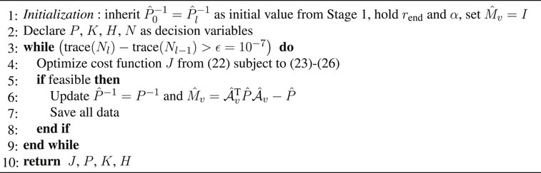
Algorithm 2 Offline Minimization of Sensitivity towards Noise (Stage 2)

5 Example: Overhead Traveling Crane

5.1 Modeling the Overhead Traveling Crane

There exist several approaches to the modeling of overhead traveling cranes, which differ in complexity due to the number of inputs. As an example, Ackermann (2002) uses a simplified model, in which the rope length change cannot be manipulated. In Park et al. (2007), the modeling of a system with variable rope length is shown. In the following model, the rope length depends on a winch whose radius has to be taken into account, leading to an extension of the model from Park et al. (2007). The crane system is shown in Figure 3 and consists of a cart that can be moved along a rail with the help of a synchronous motor. The winch drive is mounted on the cart to move the weight suspended on a rope. It is assumed that the rope has vanishing elasticity. Incremental encoders are used to measure the position of the carriage, the pendulum movement and the rope length. These are the measurable outputs of the system and can be summarized in the vector

$q={\left(x\psi l\right)}^{\mathrm{T}}.(27)$

FIGURE 3

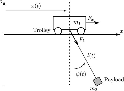
FIGURE 3. Setup of the overhead traveling crane.

The mathematical model of the overhead traveling crane is given by the derivations of the equations of motion using Lagrange’s equations of second kind. The parameters of the model are the mass m₁ = 5.5 kg of the cart, the payload with the mass m₂ = 0.5 kg, the rope winch with the radius R_T = 0.03 m and the mass moment of inertia θ = 0.000225 kg m². Then, the Lagrange function is defined as the difference of kinetic and potential energy according to

$L=E_{\mathrm{k}\mathrm{i}\mathrm{n}}-E_{\mathrm{p}\mathrm{o}\mathrm{t}}$

with the kinetic energy

$E_{\mathrm{k}\mathrm{i}\mathrm{n}}=\frac{1}{2}{\dot{x}}^2\left(m_1+m_2\right)+\frac{1}{2}{\dot{l}}^2{m}_2+\frac{1}{2}{\dot{\psi }}^2{l}^2{m}_2+\dot{x}\dot{l}{m}_2\sin \left(\psi \right)+\dot{x}\psi l{m}_2\cos \left(\psi \right)+\frac{1}{2}\theta \frac{{\dot{l}}^2}{R_{\mathrm{T}}^2}$

and the potential energy

$E_{\mathrm{p}\mathrm{o}\mathrm{t}}=-m_2\mathrm{g}l\cos \left(\psi \right),$

where the gravitation constant is g$=9.81\frac{\mathrm{m}}{{\mathrm{s}}^2}$. This leads to the second-order nonlinear state equations

$\frac{\mathrm{d}}{\mathrm{d}t}\left(\frac{\partial L}{\partial \dot{q}}\right)-\frac{\partial L}{\partial d}=Q_j,$

where Q_j represents all external and non-conservative forces, which can be summarized in the vector

$Q_j={\left(F_x-F_{\text{fc}}\dot{x}-F_{\text{fp}}\dot{\psi }{F}_l-F_{\text{fr}}\dot{l}\right)}^{\mathrm{T}}$

with the actuation forces F_x and F_l generated by the engine drum and the rope winch, respectively, as well as the friction constants of the cart $F_{\text{fc}}=13.5\frac{\mathrm{k}\mathrm{g}}{\mathrm{s}}$, the rope winch $F_{\text{fr}}=3\frac{\mathrm{k}\mathrm{g}}{\mathrm{s}}$ and the pendulum bearing $F_{\text{fp}}=0.0025\frac{\mathrm{k}\mathrm{g}}{\mathrm{s}}$. The external forces F_x and F_l are the system inputs u₁ and u₂. The resulting multivariable nonlinear equations of motion are given in Appendix A. This nonlinear model can be transformed into the quasi-linear representation

$\dot{x}=A_c\left(x\right)x+B_c\left(x\right)u,(28)$

with the state vector

$x={\left(x\dot{x}\psi \dot{\psi }l\dot{l}\right)}^{\mathrm{T}}={\left(x_1{x}_2{x}_3{x}_4{x}_5{x}_6\right)}^{\mathrm{T}}$

composed of the generalized variables (Eq. 27) and the corresponding generalized velocities $\dot{q}$. For this quasi-linear model, the simplifications

$\sin \left(\psi \right)=\psi ,\cos \left(\psi \right)=1,\mathrm{a}\mathrm{n}\mathrm{d}{\dot{\psi }}^2=0(29)$

due to small pendulum angles were made. In addition, the second input for the rope length u₂ has to be extended by $u_2^{\prime }=u_2+u_{\mathrm{2,0}}$ by the gravity compensation term u_2,0 = −m₂ g. Neglecting it would lead to a continuous increase of the rope length in the nonlinear case due to gravity.

A possible realization of the quasi-linear representation (Eq. 28) can be given by the matrices

$A_c\left(x\right)=\left(\begin{array}{cccccc}\hfill 0\hfill & \hfill 1\hfill & \hfill 0\hfill & \hfill 0\hfill & \hfill 0\hfill & \hfill 0\hfill \\ \hfill 0\hfill & \hfill -p_1\hfill & \hfill p_2\hfill & \hfill \frac{p_3}{x_5}\hfill & \hfill 0\hfill & \hfill p_4{x}_3\hfill \\ \hfill 0\hfill & \hfill 0\hfill & \hfill 0\hfill & \hfill 1\hfill & \hfill 0\hfill & \hfill 0\hfill \\ \hfill 0\hfill & \hfill \frac{p_1}{x_5}\hfill & \hfill \frac{p_5}{x_5}\hfill & \hfill \frac{p_6}{x_5^2}\hfill & \hfill 0\hfill & \hfill -p_4\frac{x_3}{x_5}-2\frac{x_4}{x_5}\hfill \\ \hfill 0\hfill & \hfill 0\hfill & \hfill 0\hfill & \hfill 0\hfill & \hfill 0\hfill & \hfill 1\hfill \\ \hfill 0\hfill & \hfill p_7{x}_3\hfill & \hfill -p_8\frac{x_4}{x_5}\hfill & \hfill 0\hfill & \hfill \frac{p_9}{x_5}\hfill & \hfill -p_{10}\hfill \end{array}\right)\mathrm{a}\mathrm{n}\mathrm{d}{B}_c\left(x\right)=\left(\begin{array}{cc}\hfill 0\hfill & \hfill 0\hfill \\ \hfill p_{11}\hfill & \hfill -p_{12}{x}_3\hfill \\ \hfill 0\hfill & \hfill 0\hfill \\ \hfill -\frac{p_{11}}{x_5}\hfill & \hfill \frac{p_{12}{x}_3}{x_5}\hfill \\ \hfill 0\hfill & \hfill 0\hfill \\ \hfill -p_{12}{x}_3\hfill & \hfill p_{13}\hfill \end{array}\right),(30)$

where the constants p_i with i = 1, 2, … , 13 consist of the system parameters. These constants and their values are given in Appendix A. It is assumed that the states x and the inputs u are constrained by

$\begin{array}{ll}\hfill x_1& \in \left[-0.5,0.5\right]\mathrm{m},x_2\in \left[-0.6,0.6\right]\frac{\mathrm{m}}{\mathrm{s}},x_3\in \left[-\frac{\pi }{6},\frac{\pi }{6}\right]\mathrm{r}\mathrm{a}\mathrm{d},\hfill \\ \hfill x_4& \in \left[-\frac{\pi }{2},\frac{\pi }{2}\right]\frac{\mathrm{r}\mathrm{a}\mathrm{d}}{\mathrm{s}},x_5\in \left[0.2,0.4\right]\mathrm{m},x_6\in \left[-0.5,0.5\right]\frac{\mathrm{m}}{\mathrm{s}}\hfill \\ \hfill u_1& \in \left[-22.5,22.5\right]\mathrm{N},u_2\in \left[-3.75,3.75\right]\mathrm{N}.\hfill \end{array}$

In general, this allows to evaluate the respective matrix entries from Eq. 30 using interval arithmetic. For the control design, a polytopic representation in the form of Eq. 9 can be defined. For that purpose, the occurring states and nonlinearities are taken into account by introducing n_δ = 5 independent parameters of the interval vector $\delta =\left[{\delta }_1,\dots ,{\delta }_{n_{\delta }}\right]$, with the components ${\delta }_i=\left[{\underline{\delta }}_i,{\bar{\delta }}_i\right]$, such that

$\begin{array}{ll}\hfill {\delta }_1& =\frac{1}{x_5}\in \left[2.5,5\right]\frac{1}{\mathrm{m}},{\delta }_2=x_3\in \left[-\frac{\pi }{6},\frac{\pi }{6}\right]\mathrm{r}\mathrm{a}\mathrm{d},{\delta }_3=\frac{x_4}{x_5}\in \left[-7.8540,7.8540\right]\frac{\mathrm{r}\mathrm{a}\mathrm{d}\mathrm{m}}{\mathrm{s}},\hfill \\ \hfill {\delta }_4& =\frac{x_3}{x_5}\in \left[-2.6180,2.6180\right]\frac{\mathrm{r}\mathrm{a}\mathrm{d}}{\mathrm{m}},{\delta }_5=-p_4\frac{x_3}{x_5}-2\frac{x_4}{x_5}\in \left[-16.3426,16.3426\right]\frac{\mathrm{r}\mathrm{a}\mathrm{d}}{\mathrm{m}\mathrm{s}}\hfill \end{array}$

which leads to the transformed matrices

$A_c\left(\delta \right)=\left(\begin{array}{cccccc}\hfill 0\hfill & \hfill 1\hfill & \hfill 0\hfill & \hfill 0\hfill & \hfill 0\hfill & \hfill 0\hfill \\ \hfill 0\hfill & \hfill -p_1\hfill & \hfill p_2\hfill & \hfill p_3{\delta }_1\hfill & \hfill 0\hfill & \hfill p_4{\delta }_2\hfill \\ \hfill 0\hfill & \hfill 0\hfill & \hfill 0\hfill & \hfill 1\hfill & \hfill 0\hfill & \hfill 0\hfill \\ \hfill 0\hfill & \hfill p_1{\delta }_1\hfill & \hfill p_5{\delta }_1\hfill & \hfill p_6{\delta }_1^2\hfill & \hfill 0\hfill & \hfill {\delta }_5\hfill \\ \hfill 0\hfill & \hfill 0\hfill & \hfill 0\hfill & \hfill 0\hfill & \hfill 0\hfill & \hfill 1\hfill \\ \hfill 0\hfill & \hfill p_7{\delta }_2\hfill & \hfill -p_8{\delta }_3\hfill & \hfill 0\hfill & \hfill p_9{\delta }_1\hfill & \hfill -p_{10}\hfill \end{array}\right)\mathrm{a}\mathrm{n}\mathrm{d}{B}_c\left(\delta \right)=\left(\begin{array}{cc}\hfill 0\hfill & \hfill 0\hfill \\ \hfill p_{11}\hfill & \hfill -p_{12}{\delta }_2\hfill \\ \hfill 0\hfill & \hfill 0\hfill \\ \hfill -p_{11}{\delta }_1\hfill & \hfill p_{12}{\delta }_4\hfill \\ \hfill 0\hfill & \hfill 0\hfill \\ \hfill -p_{12}{\delta }_2\hfill & \hfill p_{13}\hfill \end{array}\right).(31)$

If all vertices of the n_δ independent parameters of Eq. 31 are considered, the polytopic representation

$\left[A_c\left(\delta \right),B_c\left(\delta \right)\right]\in \left\{\left[A_c\left(\zeta \right),B_c\left(\zeta \right)\right]=\sum _{v=1}^{n_v}{\zeta }_v\cdot \left[A_v,B_v\right];\sum _{v=1}^{n_v}{\zeta }_v=1;{\zeta }_v\ge 0\right\}(32)$

is obtained with $n_v=2^{n_{\delta }}=32$ vertices. This allows us to taken into account the nonlinearities of the states in the controller design. The procedure described is based on Rauh et al. (2017).

Due to the independence of the parameters δ_i, the system dynamics are embedded conservatively by this approach. Reducing the pessimism should be the subject of further researches. For example, smaller interval boxes connected in series could be used to reduce the over-approximation of Eq. 31 (Azuma et al. (1997)). If all parameters δ_i are monotonically decreasing or increasing functions of x, it is also possible to reduce the number of vertices (Azuma et al. (2000)).

In the following, the first order, explicit Euler approximation

$\begin{array}{cc}\hfill A\left(\delta \right)& =A_c\left(\delta \right)T_{\mathrm{s}}+I,\hfill \\ \hfill B\left(\delta \right)& =B_c\left(\delta \right)T_{\mathrm{s}}\hfill \end{array}(33)$

with T_s = 0.015 s is used to discretize (31). This avoids the appearance of the matrix exponential function in the discretization, such that the convexity condition of Eq. 32 remains valid.

Figure 4 shows the advantage of the quasi-linear model in comparison to a linear model. For this comparison, the linear model was linearized at the operating point

$x_0={\left(00000.3\mathrm{m}0\right)}^{\mathrm{T}},u_0={\left(0u_{\mathrm{2,0}}\right)}^{\mathrm{T}}.(34)$

FIGURE 4

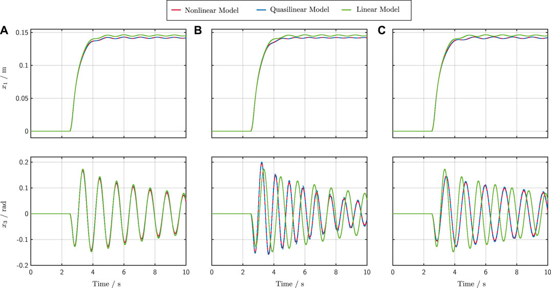
FIGURE 4. Simulation results for the nonlinear, the quasi-linear and the linear model with different rope length. Case (A) l = 0.3 m, Case (B) l = 0.2 m and Case (C) l = 0.4 m.

The nonlinear model from Appendix A is shown in red, the quasi-linear model in blue and the linear model in green. In Case (Figure 4A) all models have a constant rope length of l = 0.3 m, in Case (Figure 4B) l = 0.2 m and in Case (Figure 4C) l = 0.4 m. It can be observed that in the latter two cases large deviations occur due to the linearization and deviation from the operating point. Despite the simplifications made for small angles, a deviation from the operating point shows that the quasi-linear model behaves like the nonlinear one, while the linear model shows deviations. Due to the fact that the quasi-linear model is used, the presented approach is independent of the operating point. Only the upper and the lower bounds of the states must be known, which, however, is not a disadvantage, since these usually result from the system itself.

5.2 Control of the Overhead Traveling Crane

The presented method is to be compared with a standard approach. For this purpose, an LQG controller has been implemented additionally. Subsequently, the results of the LMI controller are compared with the standard LQG design procedure. The same control structure of both controllers ensures the comparability of the methods. Due to limited computing capacity of the implementation both controllers are linear with constant gains.

In the following, it is first described how the setting parameters of the LMI controller and the LQG controller can be selected systematically. Both LQG and LMI approaches are parameterized with the disturbance input matrices

$G_u=\left(\begin{array}{cc}\hfill 0\hfill & \hfill 0\hfill \\ \hfill 0\hfill & \hfill 0\hfill \end{array}\right),G_p=\left(\begin{array}{ccc}\hfill 0\hfill & \hfill 0\hfill & \hfill 0\hfill \\ \hfill 0.01\hfill & \hfill 0\hfill & \hfill 0\hfill \\ \hfill 0\hfill & \hfill 0\hfill & \hfill 0\hfill \\ \hfill 0\hfill & \hfill 0.01\hfill & \hfill 0\hfill \\ \hfill 0\hfill & \hfill 0\hfill & \hfill 0\hfill \\ \hfill 0\hfill & \hfill 0\hfill & \hfill 0.01\hfill \end{array}\right)\mathrm{a}\mathrm{n}\mathrm{d}{G}_y=\left(\begin{array}{ccc}\hfill 0.01\hfill & \hfill 0\hfill & \hfill 0\hfill \\ \hfill 0\hfill & \hfill 0.01\hfill & \hfill 0\hfill \\ \hfill 0\hfill & \hfill 0\hfill & \hfill 0.01\hfill \end{array}\right)$

Exactly introduced in Section 2, where the linearized model with A_nom and B_nom is used in the observer (cf. Figure 1). For that purpose, and to design the LQG controller, the nonlinear model from Appendix A has been linearized at the operating point (Eq. 34) and discretized with Eq. 33. Subsequently, the LQG’s observer and controller were designed separately from each other. In the simulation shown later, which is equivalent to Figure 1 and uses the nonlinear model from Appendix A to represent the plant, the LQG controller exhibits a stable behavior during the simulation. However, due to the nonlinearities no guaranteed stability statement can be made (invalid separation theorem). Thus, there is no proof of stability for the LQG control in the nonlinear case. Furthermore, an optimal design of the LQG controller is not possible and the parameters have to be set individually and semi-empirically. To determine the parameters as systematically as possible, the covariance matrices for the design of the observer are given by

$\begin{array}{ll}\hfill E\left[w_p\left(k\right)w_p^{\mathrm{T}}\left(k\right)\right]& =Q_o\hfill \\ \hfill E\left[w_y\left(k\right)w_y^{\mathrm{T}}\left(k\right)\right]& =R_o.\hfill \end{array}$

Furthermore, the controller parameterization in the LQG case was performed with the diagonal matrices

$\begin{array}{ll}\hfill Q_c& =\mathrm{d}\mathrm{i}\mathrm{a}\mathrm{g}\left({\mu }_{x,i}\frac{1}{x_{\mathrm{m}\mathrm{a}\mathrm{x},i}^2}\right),i=1,\dots ,n\hfill \\ \hfill R_c& =\mathrm{d}\mathrm{i}\mathrm{a}\mathrm{g}\left({\mu }_{u,j}\frac{1}{u_{\mathrm{m}\mathrm{a}\mathrm{x},j}^2}\right),j=1,\dots ,m\hfill \end{array}$

with μ_x,i = 1 and μ_u,i = 0.5.

Thus, the diagonal elements of the weighting matrices are normalized by the maximum value of the respective state or input.

For the LMI controller, there are two tuning parameters r and α, defined in Section 3.3. With these parameters, it is possible to manipulate the eigenvalue location of the extremal matrices (Eq. 31) and thus affect the dynamic behavior of the system. First, a suitable radius r is determined, with which a sufficient control gain K is available without providing high observer gains H. Therefore, α = 0 is placed and Algorithm 2 is used for various values of r. The resulting evaluation is shown in Figure 5. The parameter r represents an upper estimate of the spectral radius of all extremal matrices ${\mathcal{A}}_i$. As r decreases, the closed loop decay rate increases. Therefore, the r-dependency of the maximum time constant $T_{\mathrm{m}\mathrm{a}\mathrm{x}}({\mathcal{A}}_i)$ of all extremal matrices ${\mathcal{A}}_i$ is shown. Furthermore, Figure 5 shows the Frobenius norms of the observer ‖H‖_F gain and control gain ‖K‖_F, respectively. Since the observer gain also increases with decreasing r, a compromise between control gain and noise reduction has to be established. This compromise is represented, for example, by r = 0.993. In the following, the parameter α is investigated. Therefore, a constant distance to the stability bound is given, such that α + r = 0.993 is valid. The following four cases are subject to discussion:

$\mathrm{C}\mathrm{a}\mathrm{s}\mathrm{e}\mathrm{1}:r=0.993,\alpha =0,$

$\begin{array}{ll}\hfill & \mathrm{C}\mathrm{a}\mathrm{s}\mathrm{e}\mathrm{2}:r=0.8,\alpha =0.193,\hfill \\ \hfill & \mathrm{C}\mathrm{a}\mathrm{s}\mathrm{e}\mathrm{3}:r=0.6,\alpha =0.393,\hfill \\ \hfill & \mathrm{C}\mathrm{a}\mathrm{s}\mathrm{e}\mathrm{4}:r=0.4,\alpha =0.593.\hfill \end{array}$

FIGURE 5

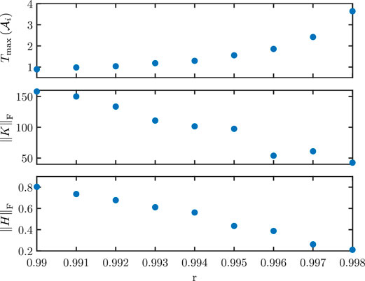
FIGURE 5. r-dependency of the maximum time constant $T_{\text{max}}({\mathcal{A}}_i)$ of all closed loop system matrices ${\mathcal{A}}_i$ and controller and observer gains, represented by ‖H‖_F and ‖K‖_F (α = 0).

Exemplarily, a simulation result for Case 2 is shown in Figure 6; Figure 7 in comparison to the LQG controller. During the simulation, a predefined, piecewise constant, tracking profile r was applied to the overhead traveling crane system. Figure 6 shows the tracking behavior and Figure 7 the observer errors. In the following, the root mean square deviations (RMSE) values

$\mathrm{\Delta }{x}_{i,C}=\sqrt{\frac{1}{N}\sum _{k=1}^N{\left(r_i\left[k\right]-x_i\left[k\right]\right)}^2},i=\mathrm{1,3,5},(35)$

$\mathrm{\Delta }{x}_{j,O}=\sqrt{\frac{1}{N}\sum _{k=1}^N{\left(x_j\left[k\right]-{\widehat{x}}_j\left[k\right]\right)}^2},j=\mathrm{2,4,6}(36)$

with N = 30 s/T_s = 2000 of the simulation shown in Figure 6; Figure 7 are taken into account. Furthermore, the maximum control variables are evaluated. For this purpose, the simulation was carried out for all four cases. The results compared to the LQG controller of this analysis are shown in Table 1.

FIGURE 6

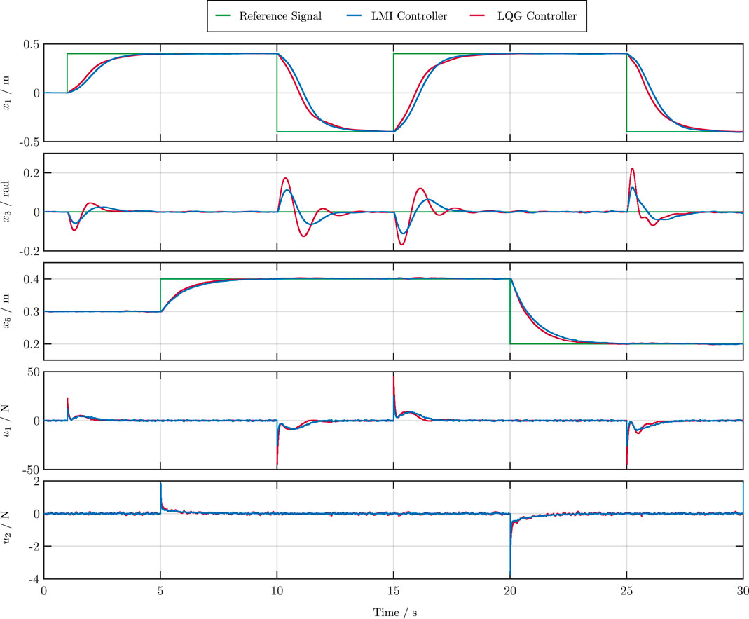
FIGURE 6. Tracking performance of the measurable states x₁, x₃ and x₅ and control inputs u₁ and u₂ for the LMI and LQG controller.

FIGURE 7

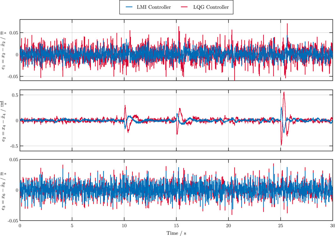
FIGURE 7. Observer errors of unmeasurable states x₂, x₄ and x₆ for the LMI and LQG controller.

TABLE 1

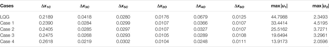
TABLE 1. Comparison of the RMSE values (Eqs 35, 36) and the maximum control variables max |u| for (α + r = 0.993).

The control performance of all four cases is similar to the LQG controller. However, the observer errors of the LMI controllers (Case 1—Case 4) are strictly smaller than the LQG observer error (see also Figure 7). Furthermore, the reduction of the radius r leads to significantly smaller control variables without negatively affecting the control and observer behavior. Next, it is shown how the optimization (Eq. 22) affects the eigenvalues of the extremal matrices. For this purpose, Figure 8 shows the respective eigenvalue locations (Case 1—Case 4) before and after the optimization. The optimization effectively suppresses system noise. The proposed algorithm achieves this by reducing the gains, thus placing the eigenvalues further to the right of the r boundary. In a final summary, a further comparison of all LMI controllers (Case 1—Case 4) to the LQG approach is shown in Table 2. Therefor, all controllers are rated in terms of the RMSE values

$\mathrm{\Delta }{\widehat{x}}_{i,f}=\sqrt{\frac{1}{N}\sum _{k=1}^N{\left({\widehat{x}}_i\left[k\right]-{\widehat{x}}_{i,f}\left[k\right]\right)}^2},i=1,\dots ,6(37)$

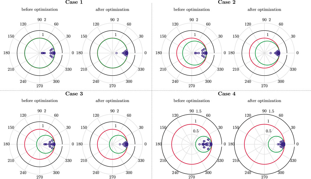
FIGURE 8

FIGURE 8. ${\mathcal{D}}_{\text{R}}$ regions before and after optimization for Case 1—Case 4.

TABLE 2

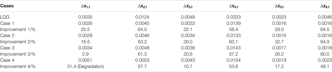
TABLE 2. Comparison for all controllers in terms of the RMSE values (Eq. 37) from all observer states ${\widehat{x}}_i$ to the ideal noise-free trajectories ${\widehat{x}}_{i,f}$; the improvement is quantified by a comparison of each Case with the LQG control.

Quantifying all observer states ${\widehat{x}}_i$ with respect to the ideal noise-free trajectories ${\widehat{x}}_{i,f}$. This comparison shows the impact of the minimization task (Eq. 22). It can be observed that the result of the minimization is degraded by progressively decreasing the radii of the ${\mathcal{D}}_{\text{R}}$ regions. This shows as well, that a compromise between decreasing the ${\mathcal{D}}_{\text{R}}$ region for the controller tuning and noise reduction has to be found. Moreover, there are significant improvements in noise reduction up to 64.9% compared to the LQG controller.

6 Conclusions and Outlook

In this article, a design of a linear observer-based state feedback controller based on an iterative LMI approach was developed for discrete-time systems in the presence of stochastic noise. Nonlinearities were taken into account by forming a polytopic quasi-linear representation. The verification of closed loop stability under disturbances could be provided by a discretized version of the Ito differential operator, whereby the noise was already taken into account in the control design. In addition, the proof of convergence for the method could be provided. The proposed method can also be applied to controllers with different structures without modifying the method. The example of the overhead traveling crane could be used to demonstrate the advantages of the new method in comparison with a standard LQG controller. This means that only a few setting parameters are required, which can be used for systematically adjusting the controller and observer gains. Furthermore, the impact of noise could be significantly reduced.

Further work will deal with an optimization of the control parameters to achieve enhanced damping properties and smaller tracking errors. This could include filter-based PID-controllers and parameter-dependent Lyapunov functions. Additionally, the observer matrices A_nom and B_nom can be optimized if they are chosen as free decision variables. On the one hand, this implies a less conservative model in which no or less unphysical vertices exist. On the other hand, the optimized observer matrices may cause unphysical behavior in control operation. This effect can be reduced, for example, by improving the convex enclosure of the quasi-linear model, similar to the interval multisection applied in Rauh et al. (2017) for the implementation of a gain-scheduling controller, such that the over-approximation is reduced. In addition, it will be investigated how actuator saturations can be included in the optimization and how they affect it.

Data Availability Statement

Data are contained within the article.

Author Contributions

Conceptualization, RD and AR; Investigation, RD, MD, SL, and AR; Software, RD, MD, SL, and AR; Validation, RD, MD, SL, AR, and BT; Writing-original draft, RD, MD, SL, AR, and BT; Writing-review and editing, RD, MD, SL, AR, and BT. All authors have read and agreed to the published version of the manuscript.

Funding

This article is funded by the Publication Fund for Open Access Publications of the University of Wuppertal.

Conflict of Interest

The authors declare that the research was conducted in the absence of any commercial or financial relationships that could be construed as a potential conflict of interest.

Publisher’s Note

All claims expressed in this article are solely those of the authors and do not necessarily represent those of their affiliated organizations, or those of the publisher, the editors and the reviewers. Any product that may be evaluated in this article, or claim that may be made by its manufacturer, is not guaranteed or endorsed by the publisher.

Acknowledgments

We acknowledge support from the Open Access Publication Fund of the University of Wuppertal.

Appendix

The nonlinear equations of the overhead traveling crane system are given by

$\begin{array}{ll}\hfill {\dot{x}}_1& =x_2\hfill \\ \hfill {\dot{x}}_2& =\frac{\left(\frac{\theta }{R_{\text{T}}^2}+m_2\right)\left(u_1-F_{\text{fc}}+F_{\text{fp}}\frac{x_4}{x_5}\cos \left(x_3\right)\right)}{m_1{m}_2+\frac{\theta }{R_{\text{T}}^2}\left(m_1+m_2-m_2{\cos }^2\left(x_3\right)\right)}\hfill \\ \hfill & +\frac{\sin \left(x_3\right)m_2\left(F_{\text{fr}}{x}_6+\frac{\theta }{R_{\text{T}}^2}{x}_4^2{x}_5-u_2+\mathrm{g}\frac{\theta }{R_{\text{T}}^2}\cos \left(x_3\right)\right)}{m_1{m}_2+\frac{\theta }{R_{\text{T}}^2}\left(m_1+m_2-m_2{\cos }^2\left(x_3\right)\right)}\hfill \end{array}$

$\begin{array}{ll}\hfill {\dot{x}}_3& =x_4\hfill \\ \hfill {\dot{x}}_4& =\frac{m_2\cos \left(x_3\right)\sin \left(x_3\right)\left(u_2-F_{\text{fr}}{x}_6\right)-\mathrm{g}\frac{\theta }{R_{\text{T}}^2}\left(1+m_1\right)-\mathrm{g}{m}_1-\frac{\theta }{R_T^2}{x}_4^2{x}_5\cos \left(x_3\right)}{x_5\left(m_1{m}_2+\frac{\theta }{R_{\text{T}}^2}\left(m_1+m_2-m_2{\cos }^2\left(x_3\right)\right)\right)}\hfill \\ \hfill & +\frac{F_{\text{fc}}{x}_2\cos \left(x_3\right)\left(\frac{\theta }{R_{\text{T}}^2}+m_2\right)-2x_4{x}_6\left(m2\frac{\theta }{R_{\text{T}}^2}+m_1\frac{\theta }{R_{\text{T}}^2}+m_1{m}_2-m_2\frac{\theta }{R_{\text{T}}^2}{\cos }^2\left(x_3\right)\right)}{x_5\left(m_1{m}_2+\frac{\theta }{R_{\text{T}}^2}\left(m_1+m_2-m_2{\cos }^2\left(x_3\right)\right)\right)}\hfill \\ \hfill & -\frac{F_{\text{fp}}\frac{x_4}{x_5}\left(\frac{\theta }{R_{\text{T}}^2}\left(1+\frac{m1}{m2}\right)-m1-m2{\cos }^2\left(x_3\right)\right)}{x_5\left(m_1{m}_2+\frac{\theta }{R_{\text{T}}^2}\left(m_1+m_2-m_2{\cos }^2\left(x_3\right)\right)\right)}\hfill \\ \hfill {\dot{x}}_5& =x_6\hfill \\ \hfill {\dot{x}}_6& =\frac{u_2\left(m_1+m_2-m_2{\cos }^2\left(x_3\right)\right)-u_1{m}_2\sin \left(x_3\right)+F_{\text{fc}}{m}_2{x}_2\sin \left(x_3\right)+m_1{m}_2{x}_4^2{x}_5}{m_1{m}_2+\frac{\theta }{R_{\text{T}}^2}\left(m_1+m_2-m_2{\cos }^2\left(x_3\right)\right)}\hfill \\ \hfill & -\frac{F_{\text{fr}}{x}_6\left(m_1+m_2+m_2{\cos }^2\left(x_3\right)\right)+F_{\text{fp}}{m}_2{x}_4\sin \left(x_3\right)\cos \left(x_3\right)-\mathrm{g}{m}_1{m}_2\cos \left(x_3\right)}{m_1{m}_2+\frac{\theta }{R_{\text{T}}^2}\left(m_1+m_2-m_2{\cos }^2\left(x_3\right)\right)}.\hfill \end{array}$

They can be simplified with (29) to the quasi-linear model (31) with the constant terms

$\begin{array}{ll}\hfill p_1& =\frac{F_{\mathrm{f}\mathrm{c}}\left(m_2+\frac{\theta }{R_{\mathrm{T}}^2}\right)}{p_{14}}=-2.3636,p_2=\frac{\mathrm{g}{m}_2\frac{\theta }{R_{\mathrm{T}}^2}+u_{\mathrm{2,0}}{m}_2}{p_{14}}=0.3567,\hfill \\ \hfill p_3& =\frac{F_{\mathrm{f}\mathrm{p}}\left(\frac{\theta }{R_{\mathrm{T}}^2}+m_2\right)}{p_{14}}=4.5455\cdot 10^{-4},p_4=\frac{F_{\mathrm{f}\mathrm{r}}{m}_2}{p_{14}}=0.2424,\hfill \\ \hfill p_5& =\frac{-\mathrm{g}\left(m_1\left(m_2+\frac{\theta }{R_{\mathrm{T}}^2}\right)+m_2\frac{\theta }{R_{\mathrm{T}}^2}\right)+u_{\mathrm{2,0}}{m}_2}{p_{14}}=2.3636,\hfill \\ \hfill p_6& =\frac{F_{\mathrm{f}\mathrm{p}}\left(\left.\frac{\theta }{R_{\mathrm{T}}^2}\frac{m_1}{m_2}+\frac{\theta }{R_{\mathrm{T}}^2}\right)\right)+m_1+\left.m_2\right)}{p_{14}}=-10.1667,p_7=\frac{F_{\mathrm{f}\mathrm{c}}{m}_2}{p_{14}}=1.0505,p_8=\frac{F_{\mathrm{f}\mathrm{p}}{m}_2}{p_{14}}=-2.02\cdot 10^{-4},p_9=\frac{\mathrm{g}{m}_1{m}_2+m_1{u}_{\mathrm{2,0}}}{p_{14}}=0,p_{10}=\frac{F_{\mathrm{f}\mathrm{r}}{m}_1}{p_{14}}=-6.6667,\hfill \\ \hfill p_{11}& =\frac{\frac{\theta }{R_{\mathrm{T}}^2}+m_2}{p_{14}}=-0.1818,p_{12}=\frac{-m_2}{p_{14}}=-0.0808,\hfill \\ \hfill p_{13}& =\frac{m_1+m_2-m_2}{p_{14}}=2.2222,p_{14}=m_1{m}_2+m_1\left(\frac{\theta }{R_{\mathrm{T}}^2}\right)=2.4750.\hfill \end{array}$

References

Ackermann, J. (2002). Robust Control. London: Springer.

Google Scholar

Azuma, T., Watanabe, R., and Uchida, K. (1997). “An Approach to Solving Parameter-dependent LMI Conditions Based on Finite Number of LMI Conditions,” in Proceedings of the American Control Conference, Albuquerque, NM, June 6, 1997. doi:10.1109/acc.1997.611851

CrossRef Full Text | Google Scholar

Azuma, T., Watanabe, R., Uchida, K., and Fujita, M. (2000). A New LMI Approach to Analysis of Linear Systems Depending on Scheduling Parameters in Polynomial Forms. at-Automatisierungstechnik 48 (4), 199. doi:10.1524/auto.2000.48.4.199

CrossRef Full Text | Google Scholar

Boyd, S., El-Ghaoui, L., Feron, E., Balakrishnan, V., and Yaz, E. (1997). Linear Matrix Inequalities in System and Control Theory. Philadelphia: SIAM: studies in applied mathematics.

Google Scholar

Coetsee, J. (1994). Control of Nonlinear Systems Represented in Quasilinear Form. Massachusetts: Massachusetts Institute of Technology.

Google Scholar

Daafouz, J., and Bernussou, J. (2001). Parameter Dependent Lyapunov Functions for Discrete Time Systems with Time Varying Parametric Uncertainties. Syst. Control. Lett. 43, 355–359. doi:10.1016/s0167-6911(01)00118-9

CrossRef Full Text | Google Scholar

de Oliveira, M. C., Bernussou, J., and Geromel, J. C. (1999). A New Discrete-Time Robust Stability Condition. Syst. Control. Lett. 37, 261–265. doi:10.1016/s0167-6911(99)00035-3

CrossRef Full Text | Google Scholar

De Oliveira, M. C., Geromel, J. C., and Bernussou, J. (2002). Extended H 2 and H Norm Characterizations and Controller Parametrizations for Discrete-Time Systems. Int. J. Control. 75, 666–679. doi:10.1080/00207170210140212

CrossRef Full Text | Google Scholar

Dehnert, R. (2020). Entwurf robuster Regler mit Ausgangsrückführung für zeitdiskrete Mehrgrößensysteme. Wiesbaden: Springer Vieweg.

Google Scholar

Dehnert, R., Lerch, S., Grunert, T., Damaszek, M., and Tibken, B. (2021). “A Less Conservative Iterative LMI Approach for Output Feedback Controller Synthesis for Saturated Discrete-Time Linear Systems,” in 25th International Conference on System Theory, Control and Computing (ICSTCC), Iasi, Romania, October 20–23, 2021. doi:10.1109/icstcc52150.2021.9607288

CrossRef Full Text | Google Scholar

Dehnert, R., Lerch, S., and Tibken, B. (2020). “Robust Anti Windup Controller Synthesis of Multivariable Discrete Systems with Actuator Saturation,” in 2020 IEEE Conference on Control Technology and Applications (CCTA), Montreal: QC, Canada, August 24–26, 2020, 581–587. doi:10.1109/ccta41146.2020.9206346

CrossRef Full Text | Google Scholar

Dehnert, R., Tibken, B., Paradowski, T., and Swiatlak, R. (2015). “Multivariable PID Controller Synthesis of Discrete Linear Systems Based on LMIs,” in 2015 IEEE Conference on Control Applications (CCA), Sydney, NSW, Australia, September 21–23, 2015, 1236–1241. doi:10.1109/cca.2015.7320781

CrossRef Full Text | Google Scholar

Furtat, I. (2018). Control of Nonlinear Systems with Compensation of Disturbances under Measurement Noises. Int. J. Control. 93, 1–23. doi:10.1080/00207179.2018.1503723

CrossRef Full Text | Google Scholar

Grunert, T., Dehnert, R., Kummert, A., Tibken, B., and Fielsch, S. (2019). “Gain Scheduled Control of Bounded Multilinear Discrete Time Systems with Uncertanties: An Iterative LMI Approach,” in 2019 IEEE 58th Conference on Decision and Control (CDC), Nice, France, December 11–13, 2019, 5199–5205. doi:10.1109/cdc40024.2019.9029623

CrossRef Full Text | Google Scholar

Ibrir, S. (2008). Static Output Feedback and Guaranteed Cost Control of a Class of Discrete-Time Nonlinear Systems with Partial State Measurements. Analysis 68 (7), 1784–1792. doi:10.1016/j.na.2007.01.011

CrossRef Full Text | Google Scholar

Kheloufi, H., Zemouche, A., Bedouhene, F., and Souley-Ali, H. (2014). “Robust H_∞ Observer-Based Controller for Lipschitz Nonlinear Discrete-Time Systems with Parameter Uncertainties,” in 53rd IEEE Conference on Decision and Control, Los Angeles, CA, December 15–17, 2014, 4336–4341.

Google Scholar

Kushner, H. J. (1967). Stochastic Stability and Control. New York: Academic Press.

Google Scholar

Lerch, S., Dehnert, R., Damaszek, M., and Tibken, B. (2021a). “Anti Windup PID Control of Discrete Systems Subject to Actuator Magnitude and Rate Saturation: An Iterative LMI Approach,” in 25th International Conference on System Theory, Control and Computing (ICSTCC), Iasi, Romania, October 20–23, 2021. doi:10.1109/icstcc52150.2021.9607157

CrossRef Full Text | Google Scholar

Lerch, S., Dehnert, R., Damaszek, M., and Tibken, B. (2021b). “Static Output Feedback Controller Design of Discrete Systems Subject to Actuator Magnitude and Rate Saturation,” in 25th International Conference on System Theory, Control and Computing (ICSTCC), Iasi, Romania, October 20–23, 2021. doi:10.1109/icstcc52150.2021.9607245

CrossRef Full Text | Google Scholar

Löfberg, J. (2004). “Yalmip: A Toolbox for Modeling and Optimization in MATLAB,” in 2004 IEEE International Conference on Robotics and Automation (IEEE Cat. No.04CH37508), New Orleans, LA, April 26–May 1, 2004 (New Orleans, LA: IEEE), 284–289.

Google Scholar

MOSEK ApS (2019). The MOSEK Optimization Toolbox for MATLAB Manual. Version 9.0. Available at: https://docs.mosek.com/9.3/faq.pdf.

Google Scholar

Park, H., Chwa, D., and Hong, K.-S. (2007). A Feedback Linearization Control of Container Cranes: Varying Rope Length. Int. J. Control Automation, Syst. 5, 379–387.

Google Scholar

Peaucelle, D., and Ebihara, Y. (2014). LMI Results for Robust Control Design of Observer-Based Controllers, the Discrete-Time Case with Polytopic Uncertainties. IFAC Proc. Volumes 47, 6527–6532. doi:10.3182/20140824-6-za-1003.00218

CrossRef Full Text | Google Scholar

Phat, V. N., and Ratchagit, K. (2011). Stability and Stabilization of Switched Linear Discrete-Time Systems with Interval Time-Varying Delay. Nonlinear Anal. Hybrid Syst. 5, 605–612. doi:10.1016/j.nahs.2011.05.006

CrossRef Full Text | Google Scholar

Ratchagit, K., and Phat, V. N. (2011). Robust Stability and Stabilization of Linear Polytopic Delay-Difference Equations with Interval Time-Varying Delays. Neural, Parallel and Scientific Computations 19, 361–372.

Google Scholar

Rauh, A., Dehnert, R., Romig, S., Lerch, S., and Tibken, B. (2021). Iterative Solution of Linear Matrix Inequalities for the Combined Control and Observer Design of Systems with Polytopic Parameter Uncertainty and Stochastic Noise. Algorithms 14, 205. doi:10.3390/a14070205

CrossRef Full Text | Google Scholar

Rauh, A., Prabel, R., and Aschemann, H. (2017). “Oscillation Attenuation for Crane Payloads by Controlling the Rope Length Using Extended Linearization Techniques,” in 2017 22nd International Conference on Methods and Models in Automation and Robotics (MMAR), Miedzyzdroje, Poland, August 28–31, 2017, 307–312. doi:10.1109/mmar.2017.8046844

CrossRef Full Text | Google Scholar

Rauh, A., Romig, S., and Aschemann, H. (2018). “When Is Naive Low-Pass Filtering of Noisy Measurements Counter-productive for the Dynamics of Controlled Systems,” in 2018 23rd International Conference on Methods Models in Automation Robotics (MMAR), Miedzyzdroje, Poland, August 27–30, 2018, 809–814.

CrossRef Full Text | Google Scholar

Rauh, A., and Romig, S. (2021). Linear Matrix Inequalities for an Iterative Solution of Robust Output Feedback Control of Systems with Bounded and Stochastic Uncertainty. Sensors 21, 3285. doi:10.3390/s21093285

PubMed Abstract | CrossRef Full Text | Google Scholar

Rauh, A., Senkel, L., Gebhardt, J., and Aschemann, H. (2014). “Stochastic Methods for the Control of Crane Systems in Marine Applications,” in 2014 European Control Conference (ECC), Strasbourg, France, June 24–27, 2014, 2998–3003. doi:10.1109/ecc.2014.6862370

CrossRef Full Text | Google Scholar

Rauh, A. (2017). Sensitivity Methods for Analysis and Design of Dynamic Systems with Applications in Control Engineering: Feedforward Control – Feedback Control – Robust Control – State Estimation. Aachen: Shaker.

Google Scholar

Sadabadi, M., and Karimi, A. (2013). An LMI Formulation of Fixed Order H_∞ and H₂ Controller Design for Discrete-Time Systems with. Polytopic Uncertainties 75, 2453–2458. doi:10.1109/CDC.2013.6760248

CrossRef Full Text | Google Scholar

Scherer, C., and Weiland, S. (1994). Linear Matrix Inequality in Control. Germany/The Netherlands: Department of Mathematics University of Stuttgart/Department of Electrical Engineering Eindhoven University of Technology.

Google Scholar

Schulz, G. (1933). Iterative Berechung der reziproken Matrix. Z. Angew. Math. Mech. 13, 57–59. doi:10.1002/zamm.19330130111

CrossRef Full Text | Google Scholar

Senkel, L., Rauh, A., and Aschemann, H. (2016). Experimental and Numerical Validation of a Reliable Sliding Mode Control Strategy Considering Uncertainty with Interval Arithmetic. Editors A. Rauh, and L. Senkel (Cham, Switzerland: Springer International Publishing), 87–122. chap. 4 part I. doi:10.1007/978-3-319-31539-3_4

CrossRef Full Text | Google Scholar

Soleymani, F. (2013). On a Fast Iterative Method for Approximate Inverse of Matrices. Commun. Korean Math. Soc. 28, 407–418. doi:10.4134/ckms.2013.28.2.407

CrossRef Full Text | Google Scholar

Wahab, A. (1994). Pole Assignment in a Specified Circular Region Using a Bilinear Transformation onto the Unit Circle. Int. J. Syst. Sci. 25 (7), 1113–1125. doi:10.1080/00207729408949265

CrossRef Full Text | Google Scholar

Yotha, N., and Mukdasai, K. (2013). New Delay-dependent Robust Stability Criterion for LPD Discrete-Time Systems with Interval Time-Varying Delays. Discrete Dyn. Nat. Soc. 2013, 929725. doi:10.1155/2013/929725

CrossRef Full Text | Google Scholar

Yucelen, T., Sadahalli, A. S., and Pourboghrat, F. (2010). “Active Noise Control in a Duct Using Output Feedback Robust Control Techniques,” in Proceedings of the 2010 American Control Conference, Baltimore, MD, June 30–July 2, 2010, 3506–3511. doi:10.1109/acc.2010.5530942

CrossRef Full Text | Google Scholar

Zemouche, A., Zerrougui, M., Boulkroune, B., Rajamani, R., and Zasadzinski, M. (2016). “A New LMI Observer-Based Controller Design Method for Discrete-Time LPV Systems with Uncertain Parameters,” in 2016 American Control Conference (ACC), Boston, MA, July 6–8, 2016, 2802–2807. doi:10.1109/acc.2016.7525343

CrossRef Full Text | Google Scholar