Bivalve Grazing Can Shape Phytoplankton Communities

Introduction

The world oceans have ~4350 phytoplankton species identified by cell morphology and likely >10 times more cryptic species (de Vargas et al., 2015), but individual phytoplankton samples usually contain fewer than 20 common taxa. The species makeup of phytoplankton communities is highly variable over time (D'Alelio et al., 2015), within (Cloern and Dufford, 2005) and between marine ecosystems (Carstensen et al., 2015). A grand challenge of aquatic ecology is developing a mechanistic understanding of the processes that select which species are present at a particular time and location. This challenge is fundamental because the ecological and biogeochemical functions of phytoplankton such as nitrogen fixation, energy transfer in food webs, and carbon export to sediments vary with phytoplankton community makeup (e.g., Litchman and Klausmeier, 2008; Boyd et al., 2010). For example, efficiency of fish production, as the ratio of fish biomass to phytoplankton biomass, is 50 times higher in diatom-based marine systems compared to cyanobacteria-dominated lakes (Brett and Muller-Navarra, 1997).

One conceptual framework of community organization is that physical-chemical environments select for different phytoplankton forms, or functional groups, on the basis of traits such as cell size, motility, and efficiency of resource acquisition (Litchman and Klausmeier, 2008). Trait-based models have been used to explain, for example: (1) dominance of picoplankton in oligotrophic ocean gyres because their small cell size (high surface:volume ratio) allows for efficient nutrient uptake in low-nutrient environments (Chisholm, 1992); (2) dominance of diatoms in coastal upwelling systems because their fast nitrate uptake supports fast growth following pulsed inputs of nitrate-rich deep water to the surface (Dugdale and Wilkerson, 1992); and (3) high biomass of dinoflagellates during periods of stratification because their motility allows migrating cells access to light energy above and nutrients below the pycnocline (Smayda and Reynolds, 2001). Central to these examples is a bottom-up view that phytoplankton communities are organized on the basis of species- or group-specific traits related to resource acquisition and growth rate.

Top-down processes play equally important roles in shaping phytoplankton communities, so trait-based models of the deep ocean also consider selection based on susceptibility of different algal taxa to consumption by pelagic grazers (Prowe et al., 2012). In shallow ecosystems such as estuaries, bays, lagoons, and littoral coastal waters, grazing by another community must be considered—benthic suspension feeders including bivalve mollusks. Bivalve grazing can be fast enough to control phytoplankton biomass in shallow coastal waters (Cloern, 1982; Kimmerer and Thompson, 2014), but we don't know if or how it plays a role in altering phytoplankton community composition. Unlike zooplankton grazing that is distributed in the water column, bivalves capture food particles from a thin boundary layer above the sediment surface. Therefore, bivalve feeding could remove some algal forms more efficiently than others based on their vertical fluxes to this boundary layer. In particular, the combined effects of benthic grazing and vertical transport (including sinking) could function as a selective process by removing sinking forms (diatoms) more efficiently than non-sinking forms.

Our interest in this hypothesis was sparked by publications suggesting that, in low-salinity habitats of San Francisco Bay, the phytoplankton community has shifted from dominance by diatoms to non-diatoms (flagellates, cyanobacteria), and this shift was caused by growing inputs of municipal sewage that elevated ammonium concentrations and N:P ratios to levels that suppress growth of diatoms relative to non-diatoms (Wilkerson et al., 2006; Dugdale et al., 2007; Glibert, 2010; Glibert et al., 2011). However, while ammonium and N:P increased steadily over time in this estuary, the decrease in diatom cell abundance and production occurred abruptly and synchronously with explosive population growth of the clam Potamocorbula amurensis after it was introduced in 1986 (Kimmerer, 2005; Cloern et al., 2015). Phytoplankton biomass and primary production declined five-fold after introduction of this non-native filter feeder (Figure 1A; Alpine and Cloern, 1992). Based on these observations, we address a fundamental question: Can bivalve suspension feeders change phytoplankton communities by removing sinking forms more efficiently than non-sinking forms? This question has general significance because it implies that phytoplankton communities in shallow coastal habitats might be structured by a different combination of processes than those operating in deep pelagic habitats. From a place-based perspective, it has important policy implications because nitrification-denitrification of sewage effluent has been mandated to reduce ammonium loadings to upper San Francisco Bay, based on the expectation that this will restore lost production of diatoms and food webs supporting endangered fishes (Wilkerson et al., 2006; Glibert et al., 2011; Dugdale et al., 2012). If the loss of diatom production was caused by other processes, such as grazing by a non-native bivalve, then this expectation might not be realized.

FIGURE 1

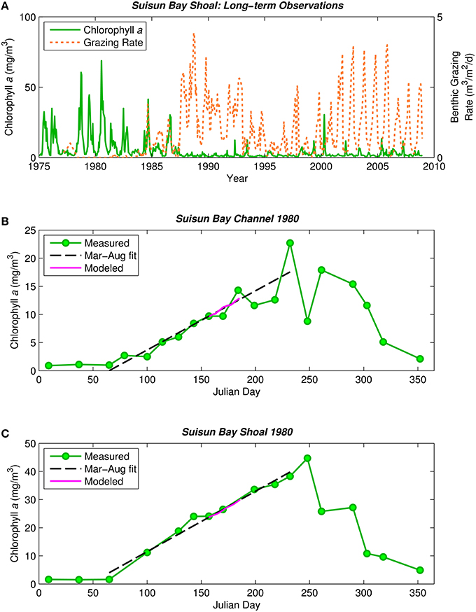
Figure 1. Historical phytoplankton biomass and bivalve grazing rates in Suisun Bay. (A) Phytoplankton biomass (1975–2009, green solid) and benthic grazing rate (1977–2009, orange dashed) in Suisun Bay shallow water. Chlorophyll a is based on water quality samples collected at Station D7 (Figure 4) by the Environmental Monitoring Program of the California Department of Water Resources (CADWR, http://www.water.ca.gov/bdma/meta/). Clam grazing rates were determined by U.S.G.S. analyses of CADWR benthic samples collected at Station D7 and samples collected by the USGS in the 1980's and 1990's at a station very close to D7. (B,C) Phytoplankton biomass measured (green) along sampling transects in Suisun Bay channel (B) and shoal (C) during year-long intensive field campaign in 1980 (Cloern et al., 1985). Dashed lines are linear fits to March-August chlorophyll a measurements. Magenta line is chlorophyll a computed by PS2D model for calibrated Suisun Bay “base case.” Computed channel chlorophyll values shown are averaged over the top 2 m of the water column and centered daily averages. Computed shoal chlorophyll values shown are depth-averages.

We used a numerical model to isolate and examine the influence of a single mechanism—bivalve grazing and its interactions with diatom sinking—on the relative proportions of sinking and non-sinking phytoplankton in shallow estuaries. We first answered a general question: Can bivalves shape phytoplankton communities based on differential rates of sinking to the benthic filtration zone? We then tailored the model to answer a place-based question: Could grazing by the introduced bivalve P. amurensis have caused a disproportionate loss of diatoms from upper San Francisco Bay?

Methods

Phytoplankton Model

We used a “pseudo-two-dimensional” phytoplankton model (“PS2D”) for this study (Lucas et al., 2009). Characterizing a vertical-lateral slice through a simplified drowned-river estuary, the model domain consists of two coupled one-dimensional (1D) water columns: one representing a narrow deep channel, and the other a broad shoal (Figure 2). Each water column of height H is discretized into a grid of cells, across which the following equation is solved using a finite volume approach:

$\begin{array}{l}\frac{\partial B}{\partial t}=\left({\mu }_{\text{net}}-ZP\right)B+\frac{\partial }{\partial z}\left(K_{\text{z}}\frac{\partial B}{\partial z}\right)\hfill \\ -\frac{\partial }{\partial z}\left(W_{\text{s}}B\right)-\frac{\partial }{\partial z}\left(BG·B\right)\hfill & \left(1\right)\hfill \end{array}$

B is phytoplankton biomass, μ_net is phytoplankton net growth rate (production minus respiration), ZP is zooplankton grazing rate, K_z is vertical turbulent diffusivity, W_s is phytoplankton sinking speed, BG is benthic grazing rate applied at the bottom boundary, z is depth from the water surface, and t is time. Lateral exchange of phytoplankton biomass between the shallow and deep domains is computed with the lateral diffusion equation:

$\begin{array}{ll}\frac{\partial B}{\partial t}=\frac{\partial }{\partial \text{y}}\left(K_{\text{y}}\frac{\partial B}{\partial y}\right)& \left(2\right)\hfill \end{array}$

The effective lateral diffusivity K_y is meant to approximately capture the net effect of hydrodynamic processes driving lateral exchange. (see Lucas et al., 2009). Model simulations of an isolated (1D vertical) channel or shoal herein simply implement a K_y value of zero. See Appendix in Supplementary Material and Tables 1, 2 for more details.

FIGURE 2

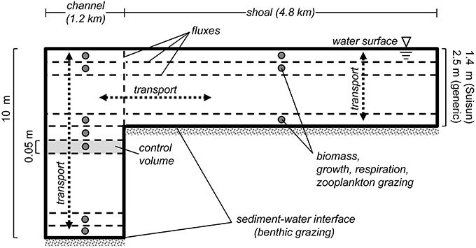
Figure 2. PS2D model schematic. Sketch describes the staggered grid layout of the PS2D phytoplankton model. The model computes phytoplankton biomass in adjacent channel and shoal water columns, which can exchange mass horizontally. Phytoplankton biomass, growth, respiration and zooplankton grazing are defined at cell (or “control volume”) centers, and advective and diffusive flux terms are computed at cell faces. Benthic grazing is treated as an advective flux at the bottom face of the bottom cell of each water column. Within each of the two water columns, phytoplankton biomass is treated as vertically variable but horizontally homogeneous. Not to scale.

TABLE 1

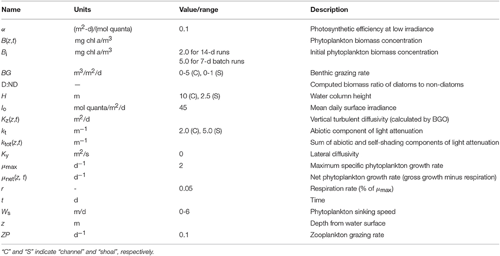
Table 1. Model variables and constants used in PS2D simulations of generic channel and shoal.

TABLE 2

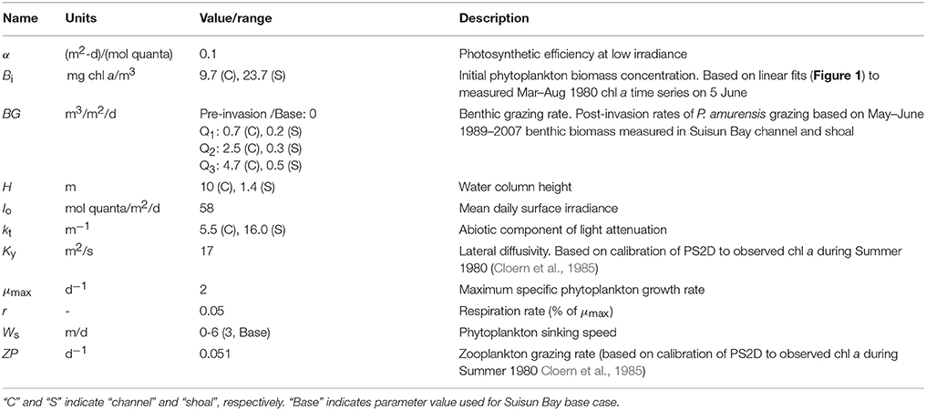
Table 2. Model variables and constants used in PS2D simulations of coupled shoal-channel depiction of Suisun Bay.

Turbulence Model

As will be shown, answers to our guiding questions are shaped by dynamics of tidally driven turbulent mixing and stratification, which affect the vertical delivery of phytoplankton. Of particular importance here is the balance between advection (sinking) and turbulent diffusion, which determines the degree to which turbulent eddies can transport negatively buoyant particles upward and thus counteract their downward flux (Lucas et al., 1998; Huisman et al., 2004). When strong stratification develops, turbulent mixing is greatly reduced and particle sinking is largely unopposed.

The influence of turbulence on phytoplankton transport is effected by K_z, the vertical turbulent diffusivity. K_z values were generated using a modified version (Monismith et al., 1996) of the 1D vertical hydrodynamic code of Blumberg et al. (1992), referred to herein as “BGO.” Time- and depth-variable K_z matrices were then read into PS2D to describe vertical mixing of phytoplankton. For this application, interaction of the tidal current with the rough bottom boundary is the primary source of turbulence, in addition to shear and buoyancy production within the water column (no wind-induced mixing is considered).

The modified BGO permits modeling of the transition between tidally-periodic and persistent stratification by varying parameters including the along-estuary salinity gradient Γ and tidal velocity U_max. If U_max is small (i.e., tidal energy is weak) and Γ is large, then gravitational circulation may develop, resulting in stratification that persists for several tidal cycles or days. If U_max is large and Γ is small, then the water column may only experience tidal-scale strain induced periodic stratification (“SIPS”; Simpson et al., 1990). This hourly scale stratification is caused by straining of vertical isopycnals by the sheared velocity profile, i.e., the transport of fresher water over saltier water during ebb tide, and the destruction of that temporary stratification during flood (Simpson et al., 1990). The deep channels of estuaries such as San Francisco Bay can experience both modes of stratification development. As implemented by Lucas et al. (2009), tidal velocity in the present study varies sinusoidally over a 14-day period to simulate spring-neap variations in tidal energy. Further details of the modified BGO and discussion of computed mixing dynamics can be found in Monismith et al. (1996), Lucas et al. (1998), Lucas et al. (2009), and the Appendix in Supplementary Material. Parameters, results, and application of all BGO runs are summarized in Table 3.

TABLE 3

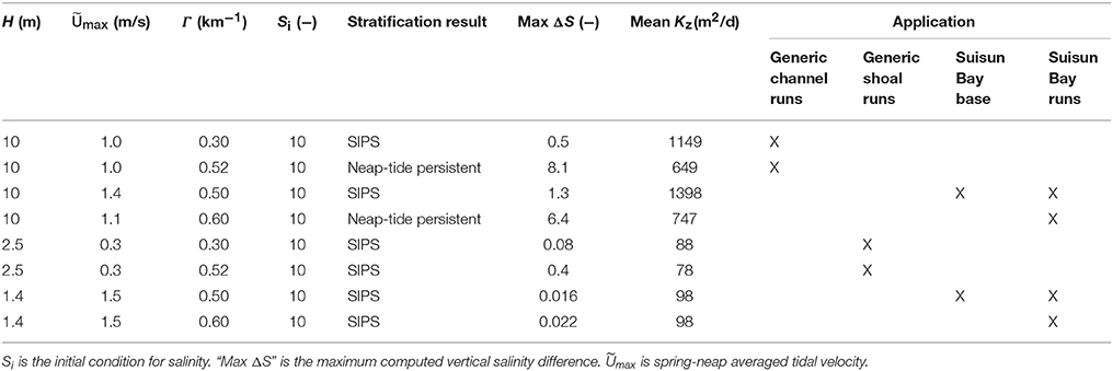
Table 3. Model parameters and scenario descriptions relevant to application of modified BGO (Blumberg et al., 1992) turbulence model for this study.

Experimental Set-Up

We applied the models described above to “generic” estuarine cases and to a case specifically designed to represent Suisun Bay. Generic cases were used to first explore fundamental processes influencing the relative proportions of sinking and non-sinking phytoplankton in representative 1D estuarine water columns. This exploration established a mechanistic foundation critical for understanding the 2D Suisun-specific simulations later on. Sinking speed was the sole characteristic distinguishing diatoms (W_s > 0) and non-diatoms (W_s = 0) in our simulations.

Generic Experiments

First, we applied the PS2D model to two separate generic cases: a 10 m deep channel and a 2.5 m deep shoal. The rationale of conducting this generic study in 1D was to first analyze interactions between sinking, grazing, light-limited growth, and vertical transport, isolated from the effects of horizontal transport between deep and shallow habitats. Both channel and shoal environments were examined because previous work (Lucas et al., 2009; Lucas and Thompson, 2012) has revealed that they can function differently. Biological model parameters for the generic runs were guided by values representative of the broader San Francisco Bay but chosen to be relevant to other estuaries as well (Table 1, Appendix in Supplementary Material). The generic study consisted of individual 14-day simulations (to dissect detailed mechanisms over a full spring-neap cycle) and 7-day batch-mode simulations, for which the model was run across multiple combinations of BG and W_s. Results of batch runs were summarized by computing the ratio of diatom to non-diatom biomass (D:ND) after 7 days.

In BGO runs for the generic channel, we varied Γ to create both a SIPS scenario and a scenario for which stratification persists through neap tide and breaks down during the higher energy spring tide. The scenarios used for the generic channel are shown in Figure 3. Computed K_z (across the vertical dimension and time) and ΔS (vertical salinity difference) are shown for the SIPS case (Figures 3B,C) and the neap-tide persistent stratification case (Figures 3D,E). Depth-averaged tidal velocity U_ave (Figure 3A) is positive for ebbs and negative for floods, and its magnitude reflects spring-neap phase. Hydrodynamic model parameters for generic channel simulations were roughly based on observations in San Francisco Bay and adjusted only to produce realistic stratification scenarios (Table 3). BGO simulations for the generic shoal implemented the same Γ values as the channel; however, given the shallowness of the modeled shoal, both Γ's resulted in SIPS for the shallow habitat (not shown). Resulting K_z profiles for the shoal were similar to Figure 3B but smaller in magnitude due to the lower shoal velocities. For the modeled shoal, higher Γ resulted in stronger tidal scale stratification (see maximum ΔS in Table 3).

FIGURE 3

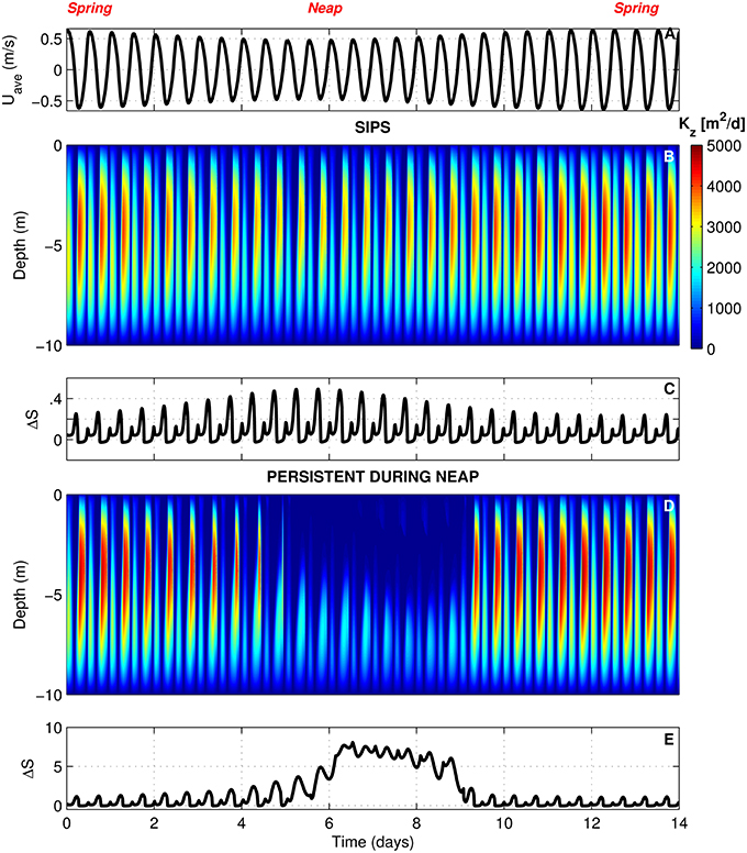
Figure 3. BGO turbulence model outputs for generic channel. (A) Depth-averaged tidal velocity (U_ave) for the SIPS case (similar to U_ave for neap-tide stratification case). (B) Computed vertical turbulent diffusivities ($K_{\text{z}}^{\prime }$s) across the vertical dimension and time for the SIPS case. (C) Vertical salinity difference (bottom minus top) for the SIPS case. (D,E) Same as (B,C), but for the case of persistent neap-tide stratification. Colorbar applies to both (B,D). See Table 3 for parameters implemented in modified BGO to generate these results.

Suisun Bay Experiments

Second, we tailored the model to represent Suisun Bay (Figure 4) as a coupled channel-shoal system (Figure 2). Our objective was to investigate whether benthic grazing could have altered the relative proportions of diatoms and non-diatoms after the 1986 Potamocorbula introduction. We first calibrated the model to observed phytoplankton biomass in Suisun Bay during the 1980 spring-summer bloom (Figures 1B,C). Wherever possible, phytoplankton model parameters for this part of the study were based on an intensive 1980 field campaign in Suisun Bay (Table 2, Appendix in Supplementary Material). Values of K_y and ZP were determined through calibration. The calibrated model represented the pre-Potamocorbula “base case” for Suisun Bay. We then performed simulations of the post-invasion period, implementing BG values based on benthos measurements in Suisun Bay after the invasion. 14-day individual and 7-day batch mode simulations were performed.

FIGURE 4

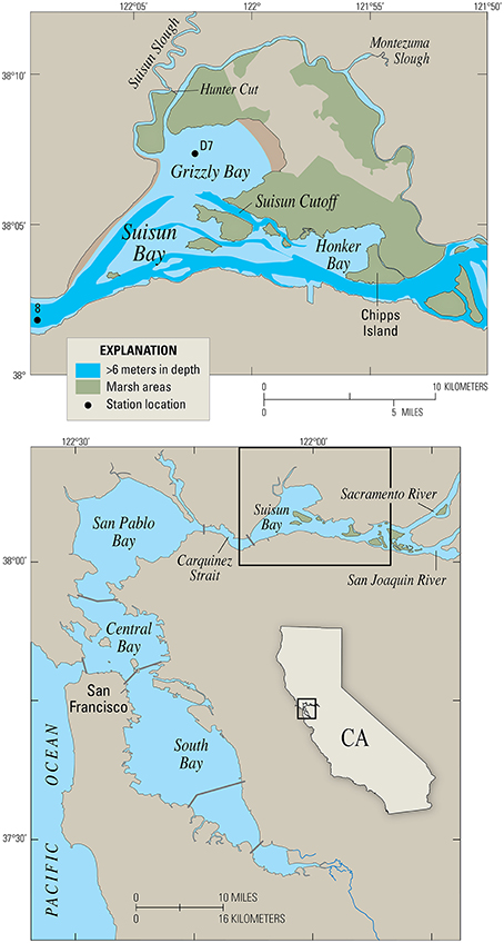
Figure 4. Map of Suisun Bay, California, the case study site. Station D7 is a long-term monitoring site for the Environmental Monitoring Program of the California Department of Water Resources. Station 8 is a long-term U.S.G.S. water quality and benthos monitoring station.

Hydrodynamic model parameters for Suisun Bay BGO runs were specifically chosen and tuned to produce tidal velocities and stratification scenarios characteristic of that environment (Table 3). Similar to the generic case, we created: (1) two hydrodynamic scenarios for the channel—tidally periodic stratification and persistent stratification during neap tide (K_z profiles not shown, but similar to those for the generic channel in Figure 3), and (2) two mixing scenarios for the shoal with Γ values matching those for the channel. Both Suisun Bay shoal scenarios resulted in SIPS due to the shallow water column.

Results

The General Problem

Generic Channel

In this section, we examine a channel environment in isolation. We begin by comparing time series of computed depth-averaged phytoplankton biomass (Figure 5) for eight 14-day simulations where the following were varied: (1) the mixing/stratification regime, (2) phytoplankton sinking speed, and (3) benthic grazing rate.

FIGURE 5

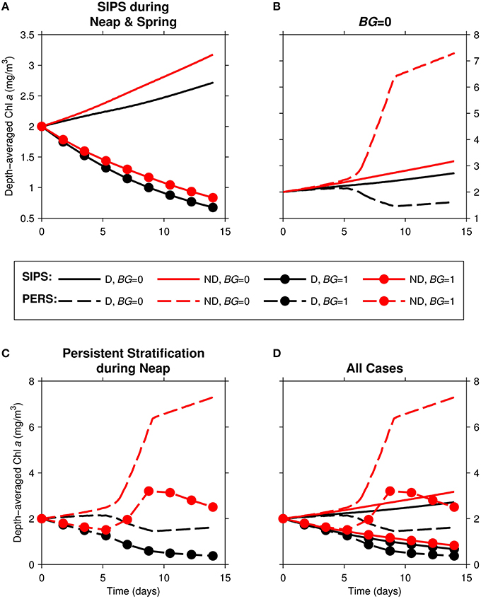
Figure 5. Time series of computed depth-averaged phytoplankton biomass for generic channel. Results from eight 14-day simulations are shown. Diatoms (“D,” black) were assigned a sinking speed of 3 m/d; non-diatoms (“ND,” red) had a sinking speed of 0 m/d. “SIPS” (solid lines) represents strain-induced periodic stratification. “PERS” (dashed lines) represents persistent neap-tide stratification. (A) SIPS (with and without benthic grazing), (B) SIPS and PERS with BG = 0, (C) PERS (with and without benthic grazing), (D) all 8 cases. Benthic grazing rate BG is in units m³/m²/d (marker if non-zero BG, no marker if zero BG).

With the relatively strong overall mixing of SIPS (Figure 5A), both diatom and non-diatom biomasses increased slowly in the absence of clam grazing and decreased with clam grazing turned on. In both grazing cases, diatom biomass was lower than non-diatom biomass. For the persistent stratification scenario in the absence of clams, non-diatom biomass increased sharply during the strong stratification period (days ~5–9), but diatom biomass decreased (Figure 5B). The addition of benthic grazing to the persistent stratification scenario (Figure 5C) resulted in a substantial decrease of both diatoms and non-diatoms compared to the no-grazing scenario. The differences between diatom and non-diatom trajectories over time for SIPS conditions were magnified by a few days of persistent stratification (the distance between black and red curves for a given BG in Figure 5A was increased by persistent stratification in Figure 5C). Overall, the highest biomass of the eight cases was achieved by non-diatoms in the scenario of persistent stratification and zero clam grazing, while the lowest overall biomass was associated with diatoms in the scenario of persistent neap-tide stratification in the presence of clams (Figure 5D).

Figure 6 provides detail across the vertical dimension and time with phytoplankton biomass contour plots for the same four persistent stratification runs shown in Figure 5C. Because the SIPS condition dominated before and after the persistent stratification episode, these cases also provide information about the effect of SIPS on phytoplankton populations.

FIGURE 6

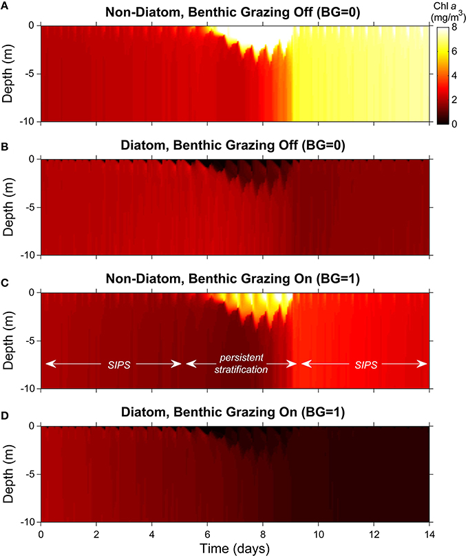
Figure 6. Phytoplankton biomass color contour plots for generic channel. Images represent variability of computed phytoplankton biomass in depth (vertical) and time (horizontal). The cases shown are the same as in Figure 5C (generic channel with persistent neap-tide stratification). Diatoms and non-diatoms were differentiated by sinking speed: W_s = 3 m/d for diatoms and 0 m/d for non-diatoms. (A) non-diatoms with zero BG (benthic grazing rate); (B) diatoms with BG = 0 m³/m²/d; (C) non-diatoms with BG = 1 m³/m²/d; (D) diatoms with BG = 1 m³/m²/d. Colorbar applies to all panels.

Without clams, non-diatom biomass grew relatively slowly overall and was largely uniform in the vertical during the early SIPS period (the initial 5-6 days; Figure 6A). When persistent stratification developed, the non-diatoms accumulated in the surface layer, where light-driven growth was maximized. When persistent stratification eroded around day 9, the high surface-layer biomass became distributed vertically, and a stratification-induced net increase in depth-averaged non-diatom biomass (relative to the pre-stratification period) was revealed. That augmented biomass increased slowly during the ensuing SIPS period. Also visible, though subtle, were brief, hourly-scale pulses of increased biomass in the upper water column, coinciding with hourly scale stratification during SIPS periods.

Diatoms exhibited much the opposite response, except for the slow overall increase during SIPS periods (Figure 6B). Neap-tide persistent stratification resulted in a loss of diatoms from the surface layer, caused by the dominance of sinking over turbulent diffusion. Once stratification broke down, any biomass left in the water column was mixed vertically, and a stratification-induced overall loss of biomass was evident, relative to the pre-stratification period (compare day ~9 to day ~5). During SIPS periods, hourly-scale pulses of decreased biomass were evident near the surface, coinciding with hourly-scale stratification.

When clam grazing was turned on, non-diatoms again accumulated in the surface layer during persistent stratification (Figure 6C). Under these conditions, loss of diatom biomass from the surface layer and its transport to the benthic grazing zone were enhanced by strong sinking that was relatively unopposed by the weakened turbulence (Figure 6D). In contrast to the BG = 0 case (Figures 6A,B), the largely well-mixed non-diatom (Figure 6C), and diatom (Figure 6D) biomass decreased slowly during SIPS periods with BG turned on. Also distinct from Figure 6B (clam grazing off), diatom biomass that sank to the lower layer in Figure 6D was available to clams for consumption, diminishing the near-bottom biomass available for resuspension when stratification broke down and resulting in very low overall biomass at the end of the simulation.

For the same cases shown in Figure 6, Figure 7 shows time series of ΔS (bottom minus top salinity) and Δchl (top minus bottom chlorophyll a). As was clear in Figure 6, the multi-day persistent stratification episode in the middle of each simulation resulted in positive Δchl for non-diatoms (because biomass built up in the surface layer) and negative Δchl for diatoms (because biomass sank out of the surface layer). Figure 7 illustrates the tidal-time scale manifestation of that same mechanism: hourly-scale variations in stratification and mixing during SIPS allowed for short-term episodes of non-diatom build-up at the surface, contrasted with diatom loss from the surface.

FIGURE 7

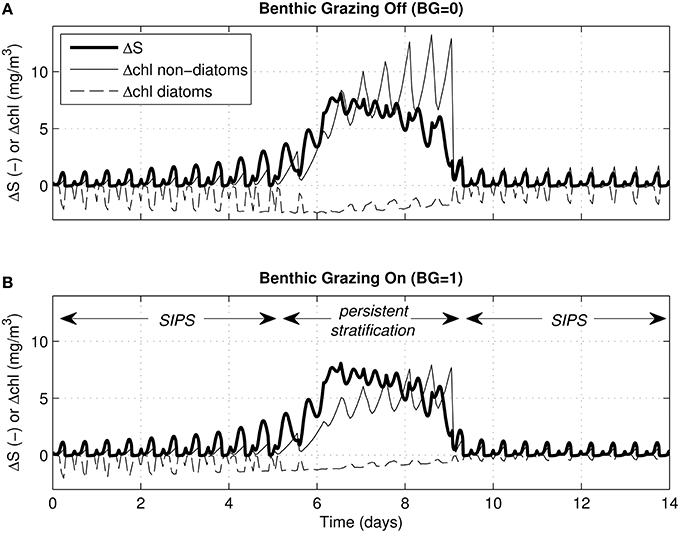
Figure 7. Vertical salinity and chlorophyll differences for generic channel. Time series of ΔS (bottom minus top salinity) and Δchl (top minus bottom chlorophyll a) are shown for the same 4 cases depicted in Figures 5C, 6A–D. For all, the water column stratified persistently during neap tide. Δchl is shown for diatoms (dashed) and non-diatoms (solid). (A) Δchl curves computed for zero benthic grazing; (B) Δchl curves computed for benthic grazing rate of 1 m³/m²/d. ΔS (bold solid) is computed by modified BGO turbulence model (same for both panels); Δchl is based on phytoplankton biomass computed by PS2D model.

Similar simulations for the generic channel were run across a two-parameter (BG and W_s) space spanning a range of BG from 0-5 m³/m²/d and W_s from 1-6 m/d for diatoms, 0 m/d for non-diatoms. The ratio D:ND is plotted as a function of BG and W_s for the cases of SIPS (Figure 8A) and persistent stratification during neap tide (Figure 8B). For both mixing scenarios, D:ND was highest in the domains of slow benthic grazing and diatom sinking, and lowest in the domains of fast benthic grazing and diatom sinking. Diatom biomass was typically <40% of non-diatom biomass in persistent stratification cases, with a maximum D:ND of 0.52. Under the SIPS scenario, the coupled effects of sinking and grazing on D:ND became less important (D:ND = 0.62-0.97).

FIGURE 8

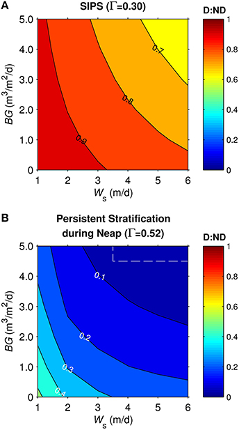
Figure 8. Diatom:non-diatom ratios (D:ND) for generic channel. D:ND is based on computed diatom and non-diatom biomass in 10 m deep channel at 7 simulation days and is shown for multiple combinations of benthic grazing rate (BG) and diatom sinking speed (W_s). (A) generic channel SIPS hydrodynamic case, (B) generic channel neap-tide persistent stratification case. Values within dashed box were calculated from computed phytoplankton biomass concentrations <0.1 mg chl a/m³, a target minimum for simulations in this study.

Generic Shoal

Dynamics in the generic shoal were generally similar to the generic channel subjected to SIPS. For example, vertical Δchl in the shoal (not shown) responded to hourly-scale variations in stratification and mixing, much like in the channel (Figure 7). D:ND patterns for the generic shoal (Figure 9) were also similar to those for the generic channel: highest D:ND was associated with the slowest sinking and benthic grazing, while lowest D:ND occurred under the fastest sinking and benthic grazing. However, simulations of the shoal habitat resulted in a broader range of D:ND ratios (e.g., 0.33-0.91 for Γ = 0.3, Figure 9A) than the channel (0.62-0.97 for Γ = 0.3, Figure 8A), even though a narrower BG range was explored for the shoal.

FIGURE 9

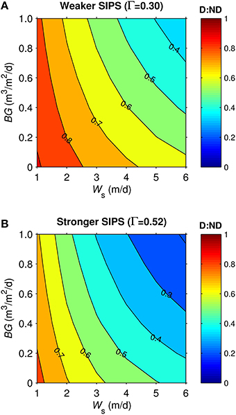
Figure 9. Diatom:non-diatom ratios (D:ND) for generic shoal. D:ND is based on computed diatom and non-diatom biomass in 2.5 m deep shoal at 7 simulation days and is shown for multiple combinations of benthic grazing rate (BG) and diatom sinking speed (W_s). (A) generic shoal SIPS case with longitudinal salinity gradient Γ = 0.30 km⁻¹ (weaker tidal-scale stratification, see Table 3), (B) generic shoal SIPS case with longitudinal salinity gradient Γ = 0.52 km⁻¹ (stronger tidal-scale stratification).

The shoal D:ND results for the two Γ values differed (Figures 9A,B). The SIPS case with the strongest Γ and thus strongest hourly-scale stratification (ΔS, see Table 3) resulted in the greatest non-diatom biomass but the lowest diatom biomass (not shown). Consequently, the different SIPS cases resulted in different D:ND ratios. For example, D:ND values in Figure 9A (with Γ = 0.3, maximum ΔS = 0.08) were on average 0.15 higher than those in Figure 9B (with Γ = 0.52, maximum ΔS = 0.4).

Application to Suisun Bay

Description of Case Study Site

Suisun Bay is a braided channel-shoal estuary, with two primary deep channels (~10–12 m deep) cutting through broad shallows and islands with typical depths of 0.3–2 m MLLW (Figure 4). Tidal range is roughly 1–2 meters, which drives currents of more than 1 m/s in the channels (Stacey et al., 2001). Currents in the shallows are reduced to 10's of cm/s (Jones and Monismith, 2008). Tidal forcing is mixed, with important contributions from the 12.4 h M2 tide and the 24 h K1 tide. During the neap tides, tidally-averaged tidal energy is reduced by roughly 20% in comparison to the springs. Typical along-estuary salinity gradients of approximately 0.5 km⁻¹ persist throughout the summer, fall and early winter (Monismith et al., 2002). The interplay between this longitudinal salinity gradient and spring-neap variability in tidal energy leads to variation in stratification conditions. Throughout the spring-neap period, stratification is typically periodic on tidal timescales, although it can persist across several tidal cycles during weak neap tides.

Suisun Bay experienced an ecological shock after the 1986 introduction of P. amurensis (Carlton et al., 1990) when the characteristic summer bloom was eliminated (Figures 1A–C) and annual phytoplankton primary production decreased five-fold (Alpine and Cloern, 1992). Before 1986, summer biomass was dominated by diatoms (e.g., Thallasiosira decipiens and Skeletonema costatum) and cryptophytes (Cloern et al., 1985; Alpine and Cloern, 1988). The abrupt decline of both phytoplankton biomass and production has been attributed to fast consumption by the introduced clam that, coupled with zooplankton grazing, can exceed phytoplankton growth rate (Kimmerer and Thompson, 2014). We used the PS2D model to explore the hypothesis that the introduction of a non-native suspension feeder could also have altered the taxonomic composition of phytoplankton by removing sinking forms more efficiently than non-sinking forms.

Case Study of Suisun Bay

The observed 1980 chlorophyll a time series in Figures 1B,C (Cloern et al., 1985) demonstrate the typical pre-Potamocorbula mode of bloom development in Suisun Bay, i.e., the long, slow growth of a bloom that began in spring and peaked in summer, with higher algal biomass in the shoals (Figure 1C) than in the deep channel (Figure 1B). Linear fits through the observed chlorophyll a time series for March-August 1980 represent that period well (see Figures 1B,C, dashed black lines). We calibrated the PS2D model to the 1980 bloom by adjusting two parameters—ZP and K_y—to best match the March–August linear chlorophyll a fits (see Appendix in Supplementary Material for additional calibration details). The model case with ZP = 0.051 1/d and K_y = 17 m²/s best matched the observed rate of biomass increase in both the channel and shoal and was thus selected as our “base case” representing pre-Potamocorbula summertime Suisun Bay (see Figures 1B,C, magenta curves).

With a calibrated Suisun-specific model in hand, we then varied sinking speed, benthic grazing rate, and the turbulent mixing/stratification scenario to explore their potential effects on the phytoplankton community in Suisun Bay. Figure 10 shows eight basic variations on the Suisun Bay base case. For base case conditions (SIPS, zero BG), modeled diatom and non-diatom biomass in the channel (Figure 10A) and shoal (Figure 10B) increased slowly over time, with diatoms increasing less rapidly than non-diatoms. Additional model runs with K_y = 0 (not shown) indicate that for these conditions both diatom and non-diatom biomass in the channel decreased if there was no hydrodynamic connection to the shoal. This is due to depth-averaged net growth rates that were negative in the channel (consistent with 1980 field observations; Cloern et al., 1985) but positive in the shoal. When benthic grazing was activated, both phytoplankton groups declined in the channel and shoal, with the diatoms decreasing most sharply (Figures 10A,B).

FIGURE 10

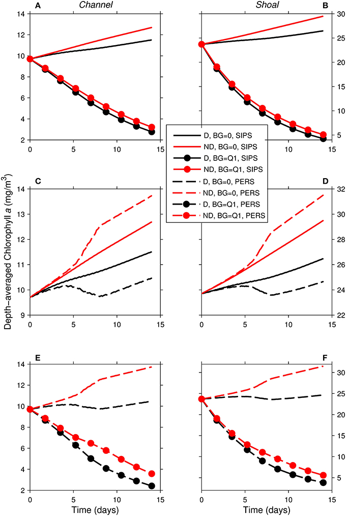
Figure 10. Time series of computed depth-averaged phytoplankton biomass for shoal-channel system representative of Suisun Bay. Results from eight 14-day simulations are shown. Diatoms (“D,” black) were assigned a sinking speed of 3 m/d; non-diatoms (“ND,” red) had a sinking speed of 0 m/d. “SIPS” (solid lines) represents strain-induced periodic stratification in the channel. “PERS” (dashed lines) represents persistent neap-tide stratification in the channel. SIPS (with and without benthic grazing) for the (A) channel and (B) shoal. SIPS and PERS with BG = 0 for the (C) channel and (D) shoal. PERS (with and without benthic grazing) for the (E) channel and (F) shoal. “Q1” indicates that the historical first quartile benthic grazing rates were used. See Table 2 for BG and other parameters implemented.

As in the isolated generic channel with zero benthic grazing (Figure 5B), diatoms and non-diatoms in the shoal-channel system had opposite responses to persistent stratification in the channel (Figures 10C,D): non-diatom biomass increased and diatom biomass decreased relative to the SIPS case. The activation of benthic grazing in the persistent stratification scenarios resulted in a substantial decrease in both diatom and non-diatom biomass compared to the no-grazing scenarios (Figures 10E,F). The differences between diatom and non-diatom trajectories over time for SIPS conditions were accentuated by persistent stratification in the channel (i.e., the distances between black and red curves for a given BG in Figures 10A,B were increased by persistent stratification in Figures 10E,F). Highest modeled biomass was achieved by non-diatoms with zero benthic grazing and neap-tide persistent stratification in the channel, while lowest total biomass was associated with diatoms under non-zero benthic grazing and persistent stratification.

Similar to the generic channel and shoal, D:ND for the coupled shoal-channel system (Figure 11) was maximized by slow sinking and benthic grazing and minimized by fast sinking and benthic grazing. System D:ND was overall higher for tidally periodic stratification in the channel (Figure 11A) than for neap-tide persistent stratification in the channel (Figure 11B; average D:ND = 0.88 for SIPS, 0.72 for persistent). Although the general trends shown in Figure 11 were similar to those for the generic channel (Figure 8) and generic shoal (Figure 9), the D:ND magnitudes for the idealized Suisun Bay system were on average higher.

FIGURE 11

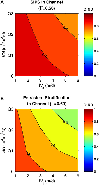
Figure 11. Diatom:non-diatom ratios (D:ND) for coupled shoal-channel system representative of Suisun Bay. D:ND is based on computed diatom and non-diatom biomass at 7 simulation days volume-integrated across the shoal-channel complex, and is shown for multiple combinations of benthic grazing rate (BG) and diatom sinking speed (W_s). (A) Suisun Bay SIPS hydrodynamic case in the channel (Γ = 0.50 km⁻¹), (B) Suisun Bay persistent neap-tide stratification in the channel (Γ = 0.60 km⁻¹). “Q1,” “Q2,” and “Q3” refer to the historical first-third quartiles for benthic grazing rate in the Suisun Bay channel and shoal (see Table 2 for BG and other parameters implemented).

Discussion

Broad Lessons

Our model-based experiments demonstrate several broadly applicable lessons:

1. Benthic filter feeding can interact with diatom sinking to alter phytoplankton community composition. Individually, the processes of benthic grazing and sinking reduce relative diatom biomass (e.g., Figures 5, 6, 8). But the maximum reduction occurs when both processes act together, as revealed in the D:ND contour plots (Figures 8, 9, 11). This finding applies to deep and shallow environments. However, the range of potential D:ND is broader for shallower habitats (Figure 9), likely due to the potentially short time scales for growth, benthic grazing, and diatom sinking in shallow water, the combination of which can result in a particularly broad range of outcomes (Lucas and Thompson, 2012).

2. The biomass ratio of sinking to non-sinking phytoplankton varies strongly with vertical mixing and stratification. The relatively vigorous mixing of a SIPS scenario (e.g., Figure 3B) provides frequent and strong coupling of a water column's upper phytoplankton source region (dominated by light-driven growth) and the lower loss region (dominated by respiration and, potentially, grazing). On the other hand, stratification weakens vertical turbulent mixing (e.g., Figures 3D,E), and if stratification persists for days, the upper layer can become essentially decoupled from the lower layer. In this situation, non-sinking phytoplankton can, to a large degree, remain in the surface layer (Huisman and Sommeijer, 2002), thereby maximizing growth and production and avoiding potentially significant losses to the benthos (Figures 6A,C; Koseff et al., 1993). The sinking of diatoms, however, can recouple the upper and lower layers of a stratified water column because turbulent eddies are not energetic enough to counteract the sinking flux (Figures 6B,D; Lucas et al., 1998; Huisman et al., 2004). In contrast to non-sinking phytoplankton, sinking forms are therefore more vulnerable to benthic grazing and spend more time in the non-productive aphotic zone when stratification is strong and persistent. The presence of persistent stratification thus has opposite effects on sinking and non-sinking forms, and can thereby set the two groups on very different trajectories over time (e.g., Figure 5B). Strong turbulent mixing, on the other hand, can result in more similar trajectories between sinking and non-sinking forms.

3. Hourly scale stratification affects sinking and non-sinking phytoplankton in opposite ways. Estuarine stratification can develop and erode over time scales of hours (as in a SIPS scenario), days, or longer. Analogous to the multi-day persistent stratification discussed above, tidally periodic stratification can also interact with phytoplankton sinking and biological processes (light-driven growth, respiration, grazing) to determine the vertical distribution of algal biomass (Figures 6, 7). For phytoplankton that do not sink, short- or long- lived stratification can produce a positive vertical chlorophyll a gradient (defined as concentration increasing upward). For phytoplankton that sink, a negative gradient can develop. The duration of these chlorophyll a gradients reflects the duration of the stratification.

Place-Based Lessons

Lessons learned from the generic channel and shoal simulations transferred to the coupled channel-shoal system designed to represent Suisun Bay. Consistent with previous work (Cloern et al., 1985), the modeled 1980 Suisun Bay was a system in which the net heterotrophic channel could not sustain a bloom without connection to the shoal, even in the absence of clams. Also consistent with previous work (Alpine and Cloern, 1992), the modeled system experienced a substantial decrease in phytoplankton biomass when benthic grazing was activated (Figure 10). Overall, our model experiments suggest that the combination of diatom sinking and filter feeding by P. amurensis could have caused a disproportionate reduction in diatom biomass relative to non-diatom biomass in this particular ecosystem (Figure 11). The average effect of the sinking-grazing mechanism on D:ND ratios for the Suisun Bay case, however, was smaller than for the generic model cases. Based on additional exploratory runs performed (not shown), this appears to be due to differences in both biological parameters and physical processes between the generic and Suisun-specific runs. Vertical mixing for the channel and shoal was on average more intense in the Suisun Bay runs (see average K_z values in Table 3), due to higher computed tidal velocities; as discussed above, more intense mixing reduces differences between sinking and non-sinking phytoplankton (i.e., raises D:ND closer to unity). Also, the Suisun Bay shoal was substantially shallower than the generic shoal, shortening the vertical mixing time scale. Differences in biological parameters (including a narrower BG range implemented for the Suisun Bay shoal than for the generic shoal) also contributed to the overall higher D:ND for Suisun Bay. D:ND is an imperfect indicator of phytoplankton community composition because it is a function of time (diatom and non-diatom biomass time series tend to diverge over time). Regardless, an important lesson from this analysis is that the balance between sinking and non-sinking phytoplankton is sensitive to both physical and biological processes.

Mechanisms

Collectively, our results suggest that the combination of diatom sinking and benthic grazing can alter the biomass ratio of sinking to non-sinking phytoplankton (D:ND). By what specific mechanism(s) does that alteration occur? One relevant metric is the ratio of phytoplankton biomass consumed by the benthos to gross biomass production (C:P) over a simulation. For the 14-day simulations performed in this study (e.g., see Figure 5), an increase in sinking speed from zero to 3 m/d in turn increased C:P in the generic channel by 9% (SIPS) and 90% (neap-tide persistent stratification). For the generic shoal, that increase in W_s amplified C:P by 20% (Γ = 0.3 km⁻¹) and 34% (Γ = 0.52 km⁻¹) with BG = 0.6 m³/m²/d. Therefore, for every unit of biomass produced, more of that biomass was consumed by the benthos if sinking was fast. Perhaps unintuitively, however, faster sinking did not necessarily translate into a greater overall quantity of phytoplankton biomass grazed by the benthos, at least over the weekly time scales modeled here. The explanation for altered D:ND ratios is more subtle than a simple expedited funneling of sinking phytoplankton into the benthos. In the following paragraphs, we dissect the individual influences of sinking and benthic grazing on phytoplankton standing stocks, describing relevant mechanisms and relative contributions.

Sinking can influence diatom standing stocks (and D:ND) by reducing the biomass produced over time. For example, with benthic grazing turned off in our generic channel, a change from W_s = 0 to 3 m/d resulted in a 13% reduction in biomass produced over 14 days under SIPS conditions and a 73% reduction if stratification persisted during neap tide (simulations shown in Figures 5A,B). This was a consequence of the sinking-induced inversion of the vertical chlorophyll gradient during periods when mixing was weak and the resulting decrease in light exposure for the diatoms. This sinking-production linkage is one mechanism shaping D:ND ratios, and highlights the importance, in some cases, of phytoplankton location within the water column as a determinant of water column productivity.

Benthic grazing also influences phytoplankton biomass by reducing gross production, even for forms that do not sink. This decrease in the phytoplankton source term appears to be due to the grazing-induced reduction in algal seed stock available for production. The magnitude of this production decrease can be comparable to or greater than the biomass grazed by the benthos over time. For example, a switch from BG = 0 to 1 m³/m²/d in our generic channel with SIPS resulted in a 47 g decrease in non-diatom biomass produced over 14 days, while only 22 g were consumed by the benthos over that same period (simulations shown in Figure 5A). Model results suggest that benthic consumption (and losses to respiration and zooplankton grazing) roughly go as production goes: if production is high (or low), then there is more (or less) available to be grazed and respired. Benthic filter feeding therefore influences phytoplankton biomass not only as a direct loss term in the chlorophyll a mass balance, but also—and just as importantly—as an indirect mechanism that reduces the source term (production).

For diatoms in the presence of filter feeding bivalves, both mechanisms for lost production are at work: decreased light exposure in the lower water column and diminishment of production seed stock by bivalve grazing. Production can become so reduced (by sinking or grazing or both) that it may no longer compensate for losses to respiration and grazing, resulting in a net heterotrophic environment.

Caveats

Of the numerous traits that differentiate phytoplankton species and groups and thus potentially influence phytoplankton communities in natural waters, we have isolated one—sinking speed—and assessed its interactions with bivalve grazing to explore their combined influence on diatom:non-diatom ratios. Diatoms have a repertoire of sinking behaviors ranging from buoyancy regulation (Waite et al., 1992) to extremely fast (100 m/d) sinking as components of aggregates (Smetacek, 1985). We used the range of sinking rates determined from measurements of vertical chlorophyll fluxes in Suisun Bay when large diatom-dominated blooms developed in summer (Ball and Arthur, 1981; Cloern et al., 1983). To understand the realized influence of the sinking-grazing mechanism in natural systems like Suisun Bay, we must consider it in the context of all the processes that influence phytoplankton communities, such as: differential growth rates among phytoplankton groups, motility, and selective grazing based on phytoplankton cell size, shape, or palatability.

Other processes and details, not considered here, could also influence results. For example, nutrient limitation and more complex representations of zooplankton grazing (e.g., distinct loss terms for micro- and mesozooplankton; Kimmerer and Thompson, 2014) have not been incorporated in the current model. For other potentially important processes, inclusion is not feasible in the pseudo-two-dimensional model construct (e.g., tidal shallowing and deepening of the water column and phasing with diel light cycles; process-based lateral transport; longitudinal transport including gravitational circulation, tidal dispersion, and riverine inputs). Turbulent mixing was idealized also in the respect that tidal asymmetry and wind were neglected.

Our PS2D characterization of the Suisun Bay case study site is further simplified in the distillation of its complex physical features into a single channel and a single shoal. Significant lateral and longitudinal bathymetric and hydrodynamic detail are thus neglected in our model, and the lack of 3D physics could influence the processes examined (Kimmerer et al., 2014). In spite of these caveats, the simplicity of this model offers the advantage of allowing the easy, efficient, and systematic examination of a limited set of relevant processes, such as the ability to switch on or off the lateral exchange between channel and shoal. This work demonstrates that useful insights can be developed and future research directions can be highlighted with simplified modeling approaches.

The Broader Context

By incorporating the effects of benthic grazing and more realistic estuarine turbulent mixing and stratification, this study extends previous model-based work that explored interactions between (more idealized) turbulent mixing, sinking, and light availability on phytoplankton community composition (e.g., Huisman et al., 2002). Those authors identified the importance of a minimum diffusivity in countering the downward advective flux of sinking phytoplankton and allowing them to persist in nature, a finding consistent with our results showing that diatoms are less competitive when stratification is strong and mixing is weak. Our incorporation of benthic grazing demonstrates how the sinking-induced decrease in production can be exacerbated by bivalve grazing. This work extends previous research probing the effects of turbulence, light availability, and benthic grazing on phytoplankton biomass (Cloern, 1991; Koseff et al., 1993; Lucas et al., 1998, 2009), by systematically exploring implications for phytoplankton community structure over a broad range of sinking rates.

The present work also delves further into the influence of tidal time scale stratification (SIPS) on phytoplankton dynamics. Simulations revealed that different SIPS mixing scenarios may result in substantial differences in phytoplankton biomass. In these simulations, the differential effect of distinct SIPS scenarios was particularly pronounced for rapidly sinking phytoplankton in shallow water (leading, for example, to the noticeably different D:ND plots for the generic shoal in Figures 9A,B). This differential effect appears related to varying strengths of hourly scale stratification (ΔS) and/or computed diffusivities. This finding departs from our previous work suggesting that different SIPS scenarios are roughly equivalent to each other and to an unstratified water column (Lucas et al., 1998). That previous research used a narrow set of conditions that did not allow for a full appreciation of the potential range of biological responses to different SIPS scenarios. A detailed and systematic exploration of the range of realistic SIPS scenarios, and their effect on phytoplankton dynamics across a broad depth-ΔS-mixing-sinking-grazing-light parameter space, is worthy of future attention.

Previous research on linkages between bivalve grazing and phytoplankton communities has focused largely on the observed effects of invasive mussels in freshwaters and, less so, on bivalve impacts in coastal systems or on modeling of those linkages. Observed responses of phytoplankton communities to benthic grazing are mixed, with studies reporting disproportionate losses of diatoms (e.g., Fahnenstiel et al., 2010), relative increases in diatom biomass (e.g., Smith et al., 1998; Petersen et al., 2008), or no significant change in phytoplankton composition (e.g., Nicholls and Hopkins, 1993) after bivalve grazer introductions. Clearly, numerous processes operate in natural systems and can confound observational analyses attempting to isolate specific drivers and responses.

Models afford control over those processes of interest and the dissection of their relative importance. Modeling of the bivalve-phytoplankton composition problem appears limited, with the work of Zhang et al. (2008) and Bierman et al. (2005) in the Great Lakes representing notable exceptions. Zhang et al. (2008) implemented a 2D model of Lake Erie and found that stronger sinking makes diatoms more vulnerable to mussel grazing than more slowly sinking algal forms. Non-diatoms were shown to increase as a result of nutrient excretion when mussel populations are large. Bierman et al. (2005) modeled the proliferation of the blue green alga Microcystis in Saginaw Bay after invasion by the zebra mussel, focusing on the processes of mussel-derived phosphorus inputs and selective grazing.

Our model-based research characterized a different kind of system: a nutrient rich, light-limited estuary with bottom-driven, tidally induced turbulence, stratification that develops and erodes over hours to days, and critical shallow-deep exchange processes. Because sinking and benthic grazing were our primary focus, our model emphasized vertical transport and variability. Although the modeled hydrodynamic processes represent shallow estuaries, our broader lessons regarding interactions of sinking and non-sinking phytoplankton with stratification, the light field, and benthic grazers should apply beyond shallow estuaries.

Conclusions

Diatoms commonly dominate phytoplankton blooms in estuarine and coastal systems, but a universal mechanistic explanation of coastal bloom dynamics—and of the dynamic composition of coastal phytoplankton communities—remains elusive (Carstensen et al., 2015). The work described herein provides one step in better understanding the broad collection of influences shaping phytoplankton community structure. We isolated and systematically examined the interactive influence of phytoplankton settling and the top-down process of bivalve grazing on phytoplankton community structure in shallow estuarine environments. Results suggest that if all else is presumed equal between diatoms and non-diatoms, differences in their sinking speeds can cause a significant and disproportionate reduction of diatom biomass, particularly in the presence of bivalve grazing. Our place-based results suggest that the sinking-grazing mechanism could have contributed to a reduction in the diatom:non-diatom biomass ratio in Suisun Bay. Details of the physical environment, such as water depth, turbulent mixing, and stratification strength and persistence, are important in modulating the relationship between benthic grazing, sinking, and phytoplankton community structure. To our knowledge, the combined influences of benthic grazing, sinking, and turbulent mixing on phytoplankton community dynamics have not been investigated experimentally (e.g., in mesocosms). That fact, combined with the simplifications inherent to our model, motivate us to view our results as hypotheses to be tested with experiments and with increasingly detailed models. Our results provide compelling evidence that the top-down process of bivalve grazing should be considered as a potentially important influence on phytoplankton communities in shallow ecosystems, and are a reminder that those communities are shaped by many interacting factors in addition to growth-regulating resources.

Author Contributions

JC and JK conceived the study. LL, JC, JT, MS, and JK all contributed to design of the study, data analysis, interpretation of data or results, and editing/revising of text. JC, JT, and LL acquired data. LL, JC, JT, and MS wrote the manuscript. LL performed model simulations and created the model-based figures.

Conflict of Interest Statement

The authors declare that the research was conducted in the absence of any commercial or financial relationships that could be construed as a potential conflict of interest.

Acknowledgments

We thank Dr. Alan Blumberg, who kindly made the original BGO code available to us, and Prof. Stephen Monismith, for his useful input in the design of this study and his many contributions to previous research foundational to this work. We are grateful to Dr. Rosanne Martyr, Dr. Antonio Olita, and Dr. Antonio Bode, whose comments improved this manuscript. This work was supported by the USGS National Research Program of the Water Mission Area and the USGS Priority Ecosystem Science Program.

Supplementary Material

The Supplementary Material for this article can be found online at: https://www.frontiersin.org/article/10.3389/fmars.2016.00014

References

Alpine, A. E., and Cloern, J. E. (1988). Phytoplankton growth-rates in a light-limited environment, San-Francisco Bay. Mar. Ecol. Prog. Ser. 44, 167–173. doi: 10.3354/meps044167

CrossRef Full Text | Google Scholar

Alpine, A. E., and Cloern, J. E. (1992). Trophic interactions and direct physical effects control phytoplankton biomass and production in an estuary. Limnol. Oceanogr. 37, 946–955. doi: 10.4319/lo.1992.37.5.0946

CrossRef Full Text | Google Scholar

Ball, M. D., and Arthur, J. F. (1981). Phytoplankton settling rates - a major factor in determining estuarine dominance (abstract). Estuaries 4, 246.

Bierman, V. J., Kaur, J., Depinto, J. V., Feist, T. J., and Dilks, D. W. (2005). Modeling the role of zebra mussels in the proliferation of blue-green algae in Saginaw Bay, Lake Huron. J. Great Lakes Res. 31, 32–55. doi: 10.1016/S0380-1330(05)70236-7

CrossRef Full Text | Google Scholar

Blumberg, A. F., Galperin, B., and O'Connor, D. J. (1992). Modeling vertical structure of open channel flows. J. Hydraul. Eng. 118, 1119–1134. doi: 10.1061/(ASCE)0733-9429(1992)118:8(1119)

CrossRef Full Text | Google Scholar

Boyd, P. W., Strzepek, R., Fu, F. X., and Hutchins, D. A. (2010). Environmental control of open-ocean phytoplankton groups: now and in the future. Limnol. Oceanogr. 55, 1353–1376. doi: 10.4319/lo.2010.55.3.1353

CrossRef Full Text | Google Scholar

Brett, M. T., and Muller-Navarra, D. C. (1997). The role of highly unsaturated fatty acids in aquatic food web processes. Freshw. Biol. 38, 483–499. doi: 10.1046/j.1365-2427.1997.00220.x

CrossRef Full Text | Google Scholar

Carlton, J. T., Thompson, J. K., Schemel, L. E., and Nichols, F. H. (1990). Remarkable invasion of San-Francisco Bay (California, USA) by the asian clam potamocorbula-amurensis.1. Introduction and dispersal. Mar. Ecol. Prog. Ser. 66, 81–94. doi: 10.3354/meps066081

CrossRef Full Text | Google Scholar

Carstensen, J., Klais, R., and Cloern, J. E. (2015). Phytoplankton blooms in estuarine and coastal waters: seasonal patterns and key species. Estaur. Coast. Shelf Sci. 162, 98–109. doi: 10.1016/j.ecss.2015.05.005

CrossRef Full Text | Google Scholar

Chisholm, S. W. (1992). “Phytoplankton size,” in Primary Productivity and Biogeochemical Cycles in the Sea, eds P. G. Falkowski and A. D. Woodhead (New York, NY: Plenum Press), 213–237.

Cloern, J. E. (1982). Does the benthos control phytoplankton biomass in South San Francisco Bay? Mar. Ecol. Prog. Ser. 9, 191–202. doi: 10.3354/meps009191

CrossRef Full Text | Google Scholar

Cloern, J. E. (1991). Tidal stirring and phytoplankton bloom dynamics in an estuary. J. Mar. Res. 49, 203–221. doi: 10.1357/002224091784968611

CrossRef Full Text | Google Scholar

Cloern, J. E., Alpine, A. E., Cole, B. E., Wong, R. L. J., Arthur, J. F., and Ball, M. D. (1983). River discharge controls phytoplankton dynamics in the Northern San Francisco Bay Estuary. Estaur. Coast. Shelf Sci. 16, 415–429. doi: 10.1016/0272-7714(83)90103-8

CrossRef Full Text | Google Scholar

Cloern, J. E., Cole, B. E., Wong, R. L. J., and Alpine, A. E. (1985). Temporal dynamics of estuarine phytoplankton: a case study of San Francisco Bay. Hydrobiologia 129, 153–176. doi: 10.1007/BF00048693

CrossRef Full Text | Google Scholar

Cloern, J. E., and Dufford, R. (2005). Phytoplankton community ecology: principles applied in San Francisco Bay. Mar. Ecol. Prog. Ser. 285, 11–28. doi: 10.3354/meps285011

CrossRef Full Text | Google Scholar

Cloern, J. E., Malkassian, A., Kudela, R., Novick, E., Peacock, M., Schraga, T. S., et al. (2015). The Suisun Bay problem: food quality or food quantity? Inter. Ecol. Progr. Newlett. 2, 15–23. Available online at: http://www.water.ca.gov/iep/docs/IEP_Vol27_1.pdf

D'Alelio, D., Mazzocchi, M. G., Montresor, M., Sarno, D., Zingone, A., Di Capua, I., et al. (2015). The green-blue swing: plasticity of plankton food-webs in response to coastal oceanographic dynamics. Mar. Ecol. 36, 1155–1170. doi: 10.1111/maec.12211

CrossRef Full Text | Google Scholar

de Vargas, C., Audic, S., Henry, N., Decelle, J., Mahé, F., Logares, R., et al. (2015). Eukaryotic plankton diversity in the sunlit ocean. Science 348, 1–12. doi: 10.1126/science.1261605

PubMed Abstract | CrossRef Full Text | Google Scholar

Dugdale, R. C., Wilkerson, F. P., Hogue, V. E., and Marchi, A. (2007). The role of ammonium and nitrate in spring bloom development in San Francisco Bay. Estuar. Coast. Shelf Sci. 73, 17–29. doi: 10.1016/j.ecss.2006.12.008

CrossRef Full Text | Google Scholar

Dugdale, R., and Wilkerson, F. (1992). “Nutrient limitation of new production in the sea,” in Primary Productivity and Biogeochemical Cycles in the Sea, eds P. G. Falkowski and A. D. Woodhead. (New York, NY: Plenum Press), 107–122.

Dugdale, R., Wilkerson, F., Parker, A. E., Marchi, A., and Taberski, K. (2012). River flow and ammonium discharge determine spring phytoplankton blooms in an urbanized estuary. Estuar. Coast. Shelf Sci. 115, 187–199. doi: 10.1016/j.ecss.2012.08.025

CrossRef Full Text | Google Scholar

Fahnenstiel, G., Pothoven, S., Vanderploeg, H., Klarer, D., Nalepa, T., and Scavia, D. (2010). Recent changes in primary production and phytoplankton in the offshore region of southeastern Lake Michigan. J. Great Lakes Res. 36, 20–29. doi: 10.1016/j.jglr.2010.03.009

CrossRef Full Text | Google Scholar

Glibert, P. M. (2010). Long-term changes in nutrient loading and stoichiometry and their relationships with changes in the food web and dominant pelagic fish species in the San Francisco Estuary, California. Rev. Fish. Sci. 18, 211–232. doi: 10.1080/10641262.2010.492059

CrossRef Full Text | Google Scholar

Glibert, P. M., Fullerton, D., Burkholder, J. M., Cornwell, J. C., and Kana, T. M. (2011). Ecological stoichiometry, biogeochemical cycling, invasive species, and aquatic food webs: San Francisco estuary and comparative systems. Rev. Fish. Sci. 19, 358–417. doi: 10.1080/10641262.2011.611916

CrossRef Full Text | Google Scholar

Huisman, J., Arrayás, M., Ebert, U., and Sommeijer, B. (2002). How do sinking Phytoplankton species manage to persist? Am. Nat. 159, 245–254. doi: 10.1086/338511

PubMed Abstract | CrossRef Full Text | Google Scholar

Huisman, J., Sharples, J., Stroom, J. M., Visser, P. M., Kardinaal, W. E. A., Verspagen, J. M. H., et al. (2004). Changes in turbulent mixing shift competition for light between phytoplankton species. Ecology 85, 2960–2970. doi: 10.1890/03-0763

CrossRef Full Text | Google Scholar

Huisman, J., and Sommeijer, B. (2002). Maximal sustainable sinking velocity of phytoplankton. Mar. Ecol. Prog. Ser. 244, 39–48. doi: 10.3354/meps244039

CrossRef Full Text | Google Scholar

Jones, N. L., and Monismith, S. G. (2008). The influence of whitecapping waves on the vertical structure of turbulence in a shallow estuarine embayment. J. Phys. Oceanogr. 38, 1563–1580. doi: 10.1175/2007JPO3766.1

CrossRef Full Text | Google Scholar

Kimmerer, W. (2005). Long-term changes in apparent uptake of silica in the San Francisco estuary. Limnol. Oceanogr. 50, 793–798. doi: 10.4319/lo.2005.50.3.0793

CrossRef Full Text | Google Scholar

Kimmerer, W. J., Gross, E. S., and MacWilliams, M. L. (2014). Tidal migration and retention of estuarine zooplankton investigated using a particle-tracking model. Limnol. Oceanogr. 59, 901–916. doi: 10.4319/lo.2014.59.3.0901

CrossRef Full Text | Google Scholar

Kimmerer, W. J., and Thompson, J. K. (2014). Phytoplankton growth balanced by clam and zooplankton grazing and net transport into the low-salinity zone of the San Francisco Estuary. Estuaries Coasts 37, 1202–1218. doi: 10.1007/s12237-013-9753-6

CrossRef Full Text | Google Scholar

Koseff, J. R., Holen, J. K., Monismith, S. G., and Cloern, J. E. (1993). Coupled effects of vertical mixing and benthic grazing on phytoplankton populations in shallow, turbid estuaries. J. Mar. Res. 51, 843–868. doi: 10.1357/0022240933223954

CrossRef Full Text | Google Scholar

Litchman, E., and Klausmeier, C. A. (2008). Trait-Based Community Ecology of Phytoplankton. Annu. Rev. Ecol. Evol. Syst. 39, 615–639. doi: 10.1146/annurev.ecolsys.39.110707.173549

CrossRef Full Text | Google Scholar

Lucas, L. V., Cloern, J. E., Koseff, J. R., Monismith, S. G., and Thompson, J. K. (1998). Does the Sverdrup critical depth model explain bloom dynamics in estuaries? J. Mar. Res. 56, 375–415.

Google Scholar

Lucas, L. V., Koseff, J. R., Monismith, S. G., and Thompson, J. K. (2009). Shallow water processes govern system-wide phytoplankton bloom dynamics: a modeling study. J. Mar. Syst. 75, 70–86. doi: 10.1016/j.jmarsys.2008.07.011

CrossRef Full Text | Google Scholar

Lucas, L. V., and Thompson, J. K. (2012). Changing restoration rules: exotic bivalves interact with residence time and depth to control phytoplankton productivity. Ecosphere 3, 117. doi: 10.1890/ES12-00251.1

CrossRef Full Text

Monismith, S. G., Burau, J. R., and Stacey, M. T. (1996). “Stratification dynamics and gravitational circulation in Northern San Francisco Bay,” in San Francisco Bay: The Ecosystem, ed J. T. Hollibaugh. (San Francisco, CA: Pacific Division of the American Association for the Advancement of Science), 123–153.

Monismith, S. G., Kimmerer, W., Burau, J. R., and Stacey, M. (2002). Structure and flow-induced variability of the subtidal salinity field in Northern San Francisco Bay. J. Phys. Oceanogr. 32, 3003–3019. doi: 10.1175/1520-0485(2002)032%3C3003:SAFIVO%3E2.0.CO;2

CrossRef Full Text | Google Scholar

Nicholls, K. H., and Hopkins, G. J. (1993). Recent changes in Lake Erie (North Shore) phytoplankton - cumulative impacts of phosphorus loading reductions and the zebra mussel introduction. J. Great Lakes Res. 19, 637–647. doi: 10.1016/S0380-1330(93)71251-4

CrossRef Full Text | Google Scholar

Petersen, J. K., Hansen, J. W., Laursen, M. B., Clausen, P., Carstensen, J., and Conley, D. J. (2008). Regime shift in a coastal marine ecosystem. Ecol. Appl. 18, 497–510. doi: 10.1890/07-0752.1

PubMed Abstract | CrossRef Full Text | Google Scholar

Prowe, A. E. F., Pahlow, M., Dutkiewicz, S., Follows, M., and Oschlies, A. (2012). Top-down control of marine phytoplankton diversity in a global ecosystem model. Prog. Oceanogr. 101, 1–13. doi: 10.1016/j.pocean.2011.11.016

CrossRef Full Text | Google Scholar

Simpson, J. H., Brown, J., Matthews, J., and Allen, G. (1990). Tidal straining, density currents, and stirring in the control of estuarine stratification. Estuaries 13, 125–132. doi: 10.2307/1351581

CrossRef Full Text | Google Scholar

Smayda, T. J., and Reynolds, C. S. (2001). Community assembly in marine phytoplankton: application of recent models to harmful dinoflagellate blooms. J. Plankton Res. 23, 447–461. doi: 10.1093/plankt/23.5.447

CrossRef Full Text | Google Scholar

Smetacek, V. S. (1985). Role of sinking in diatom life-history cycles - ecological, evolutionary and geological significance. Mar. Biol. 84, 239–251. doi: 10.1007/BF00392493

CrossRef Full Text | Google Scholar

Smith, T. E., Stevenson, R. J., Caraco, N. F., and Cole, J. J. (1998). Changes in phytoplankton community structure during the zebra mussel (Dreissena polymorpha) invasion of the Hudson River (New York). J. Plankton Res. 20, 1567–1579. doi: 10.1093/plankt/20.8.1567

CrossRef Full Text | Google Scholar

Stacey, M. T., Burau, J. R., and Monismith, S. G. (2001). Creation of residual flows in a partially stratified estuary. J. Geophys. Res. 106, 17013–17037. doi: 10.1029/2000jc000576

CrossRef Full Text | Google Scholar

Waite, A. M., Thompson, P. A., and Harrison, P. J. (1992). Does energy control the sinking rates of marine diatoms? Limnol. Oceanogr. 37, 468–477.

Google Scholar

Wilkerson, F. P., Dugdale, R. C., Hogue, V. E., and Marchi, A. (2006). Phytoplankton blooms and nitrogen productivity in San Francisco Bay. Estuaries Coasts 29, 401–416. doi: 10.1007/BF02784989

CrossRef Full Text | Google Scholar

Zhang, H., Culver, D. A., and Boegman, L. (2008). A two-dimensional ecological model of Lake Erie: application to estimate dreissenid impacts on large lake plankton populations. Ecol. Modell. 214, 219–241. doi: 10.1016/j.ecolmodel.2008.02.005

CrossRef Full Text | Google Scholar