 Robert J. Mawdsley
 Ivan D. Haigh
- Ocean and Earth Science, National Oceanography Centre Southampton, University of Southampton, Southampton, UK
Storm surges and the resulting extreme high sea levels are among the most dangerous natural disasters and are responsible for widespread social, economic and environmental consequences. Using a set of 220 tide gauges, this paper investigates the temporal variations in storm surges around the world and the spatial coherence of its variability. We compare results derived from two parameters used to represent storm surge: skew surge and the more traditional, non-tidal residual. We determine the extent of tide-surge interaction, at each study site, and find statistically significant (95% confidence) levels of tide-surge interaction at 59% of sites based on tidal level and 81% of sites based on tidal-phase. The tide-surge interaction was strongest in regions of shallow bathymetry such as the North Sea, north Australia and the Malay Peninsula. At most sites the trends in the skew surge time series were similar to those of non-tidal residuals, but where there were large differences in trends, the sites tended to have a large tidal range. Only 13% of sites had a statistically significant trend in skew surge, and of these approximately equal numbers were positive and negative. However, for trends in the non-tidal residual there were significantly more negative trends. We identified 8 regions where there were strong positive correlations in skew surge variability between sites, which meant that a regional index could be created to represent these groups of sites. Despite strong correlations between some regional skew surge indices, none were significant at the 95% level, however, at the 80% level there was significant positive correlation between the north-west Atlantic—south and the North Sea. Correlations between the regional skew surge indices and climate indices only became significant at the 80% level, where Nińo 4 was positively correlated with the Gulf of Mexico skew surge index and negatively correlated with the east Australia skew surge index. The inclusion of autocorrelation in the calculation of correlation greatly reduced their significance, especially in the short time-series used for the regional skew surge indices. Skew surge improved the representation of storm surge magnitudes, and therefore allows a more accurate detection of changes on secular and inter-annual time scales.
Introduction
Storm surges and the resulting extreme high sea levels are among the most dangerous events influencing the coastal zone (von Storch and Woth, 2008), and have been responsible for many devastating natural disasters, both in terms of loss of life (e.g., Typhoon Haiyan in November 2013) and economic losses (e.g., Hurricane Sandy in October 2012; Pugh and Woodworth, 2014). The widespread social, economic, and environmental impacts associated with such events have driven research to better understand their generating mechanisms and propagation into shallow coastal areas. However, the large number of stochastic processes that influence storm surges over a range of time and space scales, mean that they remain difficult to predict over periods longer than a few days. Understanding the risks associated with storm surges and how these might change in the future is therefore essential to aid coastal zone management and sustainable developmental planning in coastal regions (Wong et al., 2014). Using a set of 220 tide gauges, this paper builds on previous studies (e.g., Woodworth and Blackman, 2004; Menéndez and Woodworth, 2010) and assesses the regional spatial coherence of storm surges around the world and their temporal variations.
Storm surges are the response of the sea surface to forcing by the atmosphere. Several factors influence their generation and propagation into coastal waters, including: meteorological influences (i.e., wind speed, direction, persistence and spatial distribution, and sea level pressure); oceanographic effects (i.e., sea-surface temperature (SST), water density, and sea ice cover); and topographic features (i.e., water depth, width of continental shelf, as well as sand bars and reefs; Pugh and Woodworth, 2014). These characteristics are non-stationary, with variations occurring on scales from hourly to centennial, influenced by both internal natural variability and anthropogenic climate change.
Climate change could alter the frequency, intensity and tracks of storms thus influencing storm surges and extreme sea levels (Church et al., 2013). An increase in the ambient potential intensity, caused by high SST, that tropical cyclones move through should shift the distribution of intensities upwards (Seneviratne et al., 2012). However, this relationship is complicated by uncertainties concerning the response to warming (Vecchi and Soden, 2007), and the strength of counteracting mechanisms (Vecchi and Soden, 2007; Emanuel et al., 2008). As such, confidence remains low for centennial changes in tropical cyclone activity, even after accounting for past changes in observing capabilities (Hartmann et al., 2013). However, in the North Atlantic, it is virtually certain that the frequency and intensity of the strongest cyclones has increased since the 1970's (Kossin et al., 2007). Meanwhile, a net increase in frequency and intensity of extra-tropical storms, coupled with a poleward shift in storm tracks has been observed since the 1950s in both the North Atlantic and North Pacific (Trenberth et al., 2007).
The relatively short observational data set of meteorological conditions makes detecting long-term changes difficult, because of inter-annual variability (Hartmann et al., 2013). Therefore, sea level records have been often used as a proxy for storminess (e.g., Zhang et al., 2000; Araújo and Pugh, 2008; Haigh et al., 2010; Menéndez and Woodworth, 2010; Dangendorf et al., 2014), since some hourly sea level records extend back over 100 years. These studies have generally investigated changes in the non-tidal residual (NTR; the component that remains once the astronomical tidal component has been removed), or extreme sea levels (ESL; which includes changes in all components of sea level, namely, storm surges, mean sea level (MSL) and astronomical tide). The most comprehensive of these studies, by Woodworth and Blackman (2004) and Menéndez and Woodworth (2010), found that increases in ESL over the twentieth century were similar to the increases observed in MSL at most sites around the world. Further regional studies of the Mediterranean (Marcos et al., 2009), the English Channel (Araújo and Pugh, 2008; Haigh et al., 2010), the Caribbean (Torres and Tsimplis, 2013), the U.S. East Coast (Zhang et al., 2000; Thompson et al., 2013), the South China Sea (Feng and Tsimplis, 2014), had similar findings. This suggests that changes in storm surges, and therefore the meteorological conditions that drive them, were not significant over the twentieth Century and early part of the twenty-first Century, at most locations.
However, Menéndez and Woodworth (2010) did observe significant (at 95% confidence) secular trends in the NTR at a few sites. These included: increases in the Caribbean and the Gulf of Mexico; and decreases around most of Australia and parts of the east coast of the USA north of Cape Hatteras. Grinsted et al. (2012) also observed decreases in storm surge activity along the northeast US coast, but Talke et al. (2014) found evidence for an increase in annual maximum storm tide (which includes the tidal component) at New York. Significant differences between the trends in ESL and MSL have been observed for several other regions, including: the Mediterranean, at Camargue (Ullmann et al., 2007), Venice (Lionello et al., 2005), and Trieste (Raicich, 2003); the German Bight (Müdersbach et al., 2013); and sites along the western coastline of North America (Bromirski et al., 2003; Abeysirigunawardena and Walker, 2008; Cayan et al., 2008).
Many of the studies mentioned above assessed changes in ESL without separating out the tide and non-tidal components. Several recent studies have found significant trends in tidal levels and tidal constituents along the coasts of the USA or in the German Bight (e.g., Jay, 2009; Ray, 2009; Woodworth, 2010; Müdersbach et al., 2013; Mawdsley et al., 2015), and these changes in the tide may have contributed toward the observed changes in ESL at some sites. To determine changes in storm surge activity accurately any non-meteorological influence, such as non-meteorological MSL fluctuations, tidal variations and tide-surge interactions, should be removed.
Tide-surge interaction is an important component to consider and occurs for two main reasons (Horsburgh and Wilson, 2007). First, wind stress is more effective at generating storm surges at low tide, compared to high tide, because of the reduced water depth at low tide. Second, the greater water depth present during a positive surge increases the speed of tidal wave propagation, often resulting in the observed high water occurring before predicted high water (Wolf, 1981; Pugh and Woodworth, 2014). Tide-surge interaction has been most studied in the southern North Sea, where the largest positive NTR are observed to occur on the rising tide (Horsburgh and Wilson, 2007). Tide-surge interactions have also been observed across other continental shelf regions and in shallow water areas, including: the English Channel (Haigh et al., 2009b; Idier et al., 2012); Canada (Bernier and Thompson, 2007); Australia (Haigh et al., 2014); the South China Sea (Feng and Tsimplis, 2014); the Bay of Bengal (Antony and Unnikrishnan, 2013); and was observed during Hurricane Sandy off the USA east coast (Valle-Levinson et al., 2013). However, the extent to which tide-surge interactions occur has not been assessed for large stretches of the world's coastline.
Recently, several studies have used the parameter “skew surge,” rather than the traditional NTR, to assess ESL in north-west Europe (Batstone et al., 2013; Dangendorf et al., 2014), and in the USA (Wahl and Chambers, 2015). A skew surge is the difference between the maximum observed sea level and the maximum predicted tidal level regardless of their timing during the tidal cycle. There is one skew surge value per tidal cycle. A skew surge is thus an integrated and unambiguous measure of the storm surge that represents the true meteorological component of sea level (Haigh et al., 2015). For the UK, Batstone et al. (2013) found that variations in skew surge heights are independent of the tidal level, and therefore by using them, one does not have to consider the complications of non-linear tide-surge interactions.
Whatever parameter is used, understanding changes in storm surge requires analysis of low frequency variability, which can have a considerable effect on storm surge conditions. This is often done by comparing storm surge parameters to regional climatic variations, by the use of simple indices, typically based on sea level pressure (SLP) or SST and gives a simplified description of the regional climatic conditions.
The El Niño Southern Oscillation (ENSO) has one of the most widespread influences on climate variability, stretching across the Pacific and into the Atlantic. For example, the number of hurricanes in the Atlantic is known to reduce during strong El Nińo events (Bell and Chelliah, 2006). However, Menéndez and Woodworth (2010) found a small positive correlation between the Nińo 3 index and the magnitude of the NTR at sites between Cape Hatteras and Cape Cod. In the Caribbean, Torres and Tsimplis (2013) found that 2 out of the 5 sites they studied were anti-correlated with ENSO, but Menéndez and Woodworth (2010) found no significant relationship. Woodworth and Menéndez (2015) found that ESL largely followed the pattern of MSL response to ENSO. By contrast, the tropical west Pacific and the coast of Australia showed a negative correlation (Feng and Tsimplis, 2014). Positive correlation was observed between ENSO, the number of storms that make landfall (Feng and Tsimplis, 2014) and the magnitude of the NTR (Menéndez and Woodworth, 2010) in China, although Feng and Tsimplis (2014) found that neither ENSO nor the Pacific Decadal Oscillation (PDO) was an indicator of a change in magnitude of ESL. Elsewhere in the Pacific, increases in ESL at sites in British Columbia were attributed to a strong positive trend in the PDO (Abeysirigunawardena and Walker, 2008).
In the North Atlantic, the North Atlantic Oscillation (NAO) is the most dominant regional climate signal. Marcos et al. (2009) found that the median and higher percentiles of sea level were both strongly correlated with NAO. However, the correlation between NAO and the NTR was weaker. Haigh et al. (2010) showed that there was a weak negative correlation to the winter NAO throughout the English Channel and a stronger significant positive correlation at the boundary with the southern North Sea. This latter finding is supported by Menéndez and Woodworth (2010) who found a positive correlation of the Arctic Oscillation (AO) and NAO, for most sites around the UK (but not the English Channel) and Scandinavia. In the eastern Atlantic, Talke et al. (2014) and Ezer and Atkinson (2014) both observed anti-correlation between NAO and their different measures of ESL.
In summary, although much research has been conducted to determine the temporal variability of storm surge activity on decadal and longer time-scales, the majority of past studies have focused on the NTR. Skew surges can quantify the meteorological component of sea level better, by removing the impact of phase offsets and tide-surge interactions. However, until now (to our knowledge) they have only been used to assess changes in storm surge activity around north-west Europe and USA. Little research has been conducted into tide-surge interaction in many regions, and therefore it would be prudent to identify further regions where this may have an important impact on the magnitude of ESL. Furthermore, few studies have examined the spatial coherence in storm surge variability along stretches of coastlines and between regions. This is despite the fact that regional climatic variability can account for much of the inter-annual and multi-decadal variability in storm surges (Marcos et al., 2015; Wahl and Chambers, 2016).
Therefore, the overall aim of this paper is to assess the spatial and temporal variations in storm surge activity (and thus infer changes in storminess) over the twentieth century and early part of the twenty-first century at a quasi-global scale, addressing the issues highlighted above. We build on two comprehensive global studies undertaken by Woodworth and Blackman (2004) and Menéndez and Woodworth (2010) and utilize an updated version of their Global Extreme Sea Level Analysis (GESLA) tide gauge dataset (Mawdsley et al., 2015). We have four specific objectives. Our first objective is to determine the extent of tide-surge interaction, at each of our 220 study sites, as this determines the scale of the differences between skew surge and NTR values. Our second objective is to compare how the use of skew surge or NTR, effects the assessment of storm surge activity. Our third objective is to assess the extent to which there is spatial coherence in skew surge variability, both locally (i.e., between adjacent tide gauge sites) and regionally (i.e., across ocean basins). Our fourth and final objective is to compare inter-annual and multi-decadal variations in skew surge with fluctuations in regional climate.
The format of the paper is as follows. The data and methodology are described in Sections Data and Methodology, respectively. The results for each of the four objectives are presented in Section Results in turn. Key findings are discussed in Section Discussion and conclusions are given in Section Conclusions.
Data
High-resolution (i.e., at least hourly) sea level data is required to analyse storm surge characteristics. The most comprehensive high frequency sea level dataset available is the GESLA database. This dataset was originally collated by staff from the National Oceanography Centre (NOC) in the UK and the Antarctic Climate and Ecosystems Cooperative Research Centre (ACECRC) in Australia. The GESLA dataset has primarily been used to assess changes in ESL (e.g., Woodworth and Blackman, 2004; Menéndez and Woodworth, 2010; Hunter, 2012; Hunter et al., 2013; Marcos et al., 2015) but has also been used to evaluate changes in the tides (Woodworth, 2010; Mawdsley et al., 2015).
We have extended the original GESLA dataset, to include additional sites and updated the records to the end of 2014 (see Mawdsley et al., 2015 for details). Many records in the GESLA dataset were excluded from this analysis by a number of criteria designed to ensure that data were of sufficient length and quality for robust analysis. These criteria are detailed in Mawdsley et al. (2015) and resulted in 220 eligible sites, the locations of which are shown in Figure 1 (and documented in the Supplementary Material). The sites used in this study were determined by the needs of the previous study on change in tidal levels (Mawdsley et al., 2015) and hence sites in the Mediterranean and Baltic seas have not been used, because the tide was too small to be analyzed on an annual basis in these areas. We conducted further quality control on all records to ensure any remaining spikes, or datum and phase offsets were flagged and excluded from the analysis. Data clearly affected by tsunamis were also removed, since the occurrence of these non-climate related events are unpredictable and can affect results. Small tsunami signals are difficult to separate from the NTR, and therefore some events remain in the dataset. Tide gauge measurements are deemed acceptable if they have an accuracy of less than 1 cm, according to the Inter-governmental Oceanographic Commission (IOC; 2006). Many modern day instruments are accurate to approximately 3 mm, but all instruments used in this study will meet the minimum requirements of the IOC.
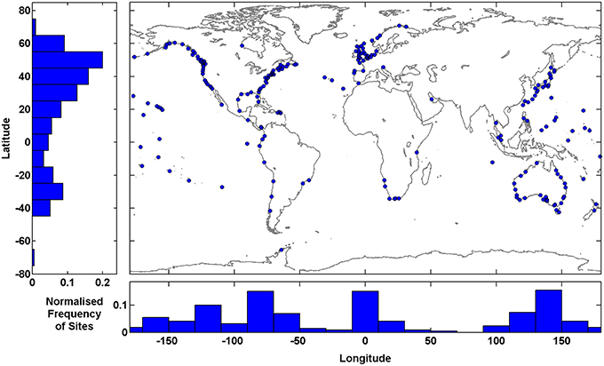
Figure 1. Location map of 220 selected sites used in the analysis. Normalized frequency histograms are plotted along the x-axis for longitude and y-axis for latitude.
We used 8 climate indices: the Atlantic Multi-decadal Oscillation (AMO), AO, NAO, Nińo 3, Nińo 4, North Pacific (NP), PDO, Southern Oscillation Index (SOI). The NAO index was downloaded from the Climate Research Unit of the University of East Anglia (https://crudata.uea.ac.uk/cru/data/nao/nao.dat). The other indices were obtained from the National Oceanic and Atmospheric Administration (NOAA) (http://www.cpc.ncep.noaa.gov).
Methodology
At each of the 220 study sites, the observed sea level record was separated into its three main component parts for each year: MSL, tide and NTR (Pugh and Woodworth, 2014). We followed the same method as detailed in Mawdsley et al. (2015), and used their technique for extracting the time and magnitude of tidal high waters (HW), from here on described as predicted HW. For every predicted HW at each site, we calculated a skew surge value. Batstone et al. (2013) used a method that identified the maximum predicted and observed water levels between successive low waters. However, we found this approach was not appropriate in mixed tidal regimes, and given the global nature of this study we developed another method that works across all tidal regimes. We calculated skew surges by finding the largest local maxima in the observed sea level, within a ±3 h window of the time of each predicted HW (Figure 2). Most observed HW occurred within this window, but if no observed HW were found during this window we extended it to ±6 h. In a mixed tidal regime, the coupling of each observed HW to each predicted HW is more complicated. Therefore, we introduced two criteria to ensure that the observed HW is primarily caused by the predicted HW to which it is coupled. Firstly, if the predicted HW is between double low tides we do not assign an observed HW. Secondly, if a second predicted HW is closer in time to an observed HW than its coupled predicted HW, we remove the coupling between that predicted and observed HW. These caveats mean that some predicted HW did not have an associated observed HW, but this method captured a mean of 95% of observed HWs at all sites. Two sites (Bunbury and Hoek van Holland) had an observed HW assignment less than 80%, because many observed HWs occurred around double low tides and were removed.
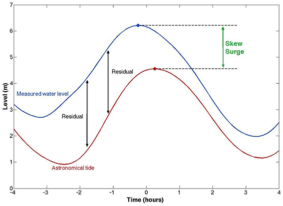
Figure 2. Schematic example of a storm surge event and the different calculation methods for the NTR and skew surge.
We then examined the differences between the skew surge and NTR time series, at each of our 220 study sites, and determined the extent of tide-surge interaction. Initially we compared the maximum values of skew surge and NTR from the entire time series, where concurrent values in both time series occur for an event at each site. For example, the maximum NTR at Galveston, USA was generated by Hurricane Ike in September 2008, however, the tide gauge broke just before the predicted HW and no corresponding skew surge value for this particular tidal cycle could be calculated. We also compared the maximum skew surge value with the maximum NTR at high water (if tide-surge interaction is negligible you would expect these two values to be the same). We used the chi-squared (χ2) test, which was first used for sea level studies by Dixon and Tawn (1994) but was modified by Haigh et al. (2010) to quantify the level of tide-surge interaction at each site. The χ2 test calculates the probability that the observed dataset is different to an expected dataset. In this case, if the two are different then it demonstrates that tide-surge interaction is significant. Dixon and Tawn's (1994) approach, from here on called the tidal-level method, involved splitting the astronomical tidal range into five equi-probable bands. If the tide and NTR were independent processes, the number of NTR per tidal band would be equal, but if interaction is significant the number of NTR per tidal band would differ. As Haigh et al. (2010) pointed out, this method does not distinguish that interaction tends to be different on the ebb and flood phases of the tide (Horsburgh and Wilson, 2007). Haigh et al. (2010) therefore modified the method to compare the relative timing of the peak NTR to the predicted HW, and this method is from here on called the tidal-phase method. The tide was divided into 13 hourly bands between 6.5-h before and after high water. With no tide–surge interaction the expected number of occurrences in each of the 13 bands would be the same. See Haigh et al. (2010) for the mathematical details. We use the same 13 hourly bands to assess tide-surge interaction in the tidal-phase method, but use 6 equi-probable bands for the tidal-level. The results from both methods are based on the largest 200 NTR events, where an event is defined by a 72-h window centered on the peak NTR, to ensure that each NTR peak is independent. Statistical significance for the χ2 test is given for a p < 0.05.
Next, we assessed the long-term trends in skew surge time-series, at each site and compared these to trends calculated from the NTR time-series. We used the percentiles method (e.g., Haigh et al., 2010; Menéndez and Woodworth, 2010), which ranks the parameter values for each year. The 50th percentile of the NTR time-series (the median) approximates to zero, while the 99.9th percentile is about the level of the 8th highest hourly sea level value. For skew surges, the tidal regime at each site affects the annual number of HWs. In semi-diurnal regimes there are approximately 705 skew surge values a year, whereas for a diurnal regime an average of 352 skew values would occur. Therefore, the 99th percentile represents a value between the 4th and 7th highest values in the skew surge time series. Trends were calculated for these percentiles, using linear regression, while standard errors were estimated using a Lag-1 autocorrelation function to allow for any serial autocorrelation in the time-series (Box et al., 1994). From here on, when we use the term “significant trends,” this signifies that the trends are statistically (at 95% confidence level) different from zero.
We chose high percentiles because they represent the largest events at each site, but the inter-annual variability present in the higher percentile time-series can obscure the inter-decadal variability and secular trends. To assess the extent to which there is spatial coherence in skew surge variability, we calculated a correlation coefficient between the skew surge percentile time-series for each pair of sites. We identified groups of sites, along a stretch of coastline, where the correlation between them was high, and designated them as coherent regions. We created regional skew surge indices by calculating the mean of the de-trended and normalized time-series of the 99th percentile of skew surge for each site in that area. We only derived regional indices for the period from 1970 to 2010, when there was sufficient overlap of data among sites in each region, but increase the temporal comparison by comparing individual long-time series from each region. We filtered the regional skew surge indices using a locally regressed least squares (Loess) approach (Cleveland and Devlin, 1988), which through testing gave the lowest standard error. This non-parametric method combines a multiple regression model with a nearest-neighbor model. Each point of the loess curve was fitted using local regression, using a 2nd degree polynomial to the points within a 10-year window centered on that point. These filtered time-series are used to assess the temporal variations in the regional skew surge indices and the correlation of those indices between each other and against the regional climate indices, listed in Section Data. The significance of the correlation between the different regional skew surge indices and between them and the climate indices, is determined by using the Lag-1 autocorrelation function (Box et al., 1994).
Results
Tide-Surge Interactions
Our first objective was to identify any tide-surge interaction, at each of the 220 study sites, and we did this using the 4 methods detailed in Section Methodology. The difference between the maximum skew surge value and the maximum NTR over the whole time series, is shown for each site in Figure 3A. We expect small differences at sites where tide-surge interaction is negligible. Results shows that the difference is predominantly largest in regions surrounded by shallow bathymetry, such as the German Bight, Northern Australia, the Gulf of Panama and parts of the east coast of North America. However, there are other sites with large differences, including: sites in northern Australia (Port Hedland, Broome, Wyndham, Townsville and Bundaberg); Easter and Wake Islands in the Pacific Ocean; Funchal on Madeira, Portugal; and Yakutat in Alaska. At 120, 80, and 20 sites, the difference is larger than 10, 20, and 50 cm, respectively. When we calculate the difference between the maximum skew surge and the maximum NTR observed at the time of predicted HW we find that 137 sites have a value of zero, as shown in Figure 3B. However, sites in the North Sea, the US east coast, north-west Australia and a few other individual locations have non-zero values which suggests that in these regions the tide-surge interaction shifts the peak in NTR away from predicted HW.
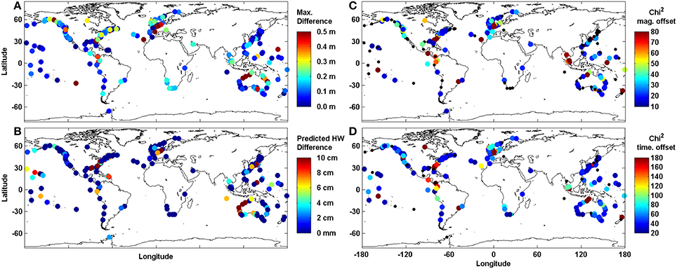
Figure 3. Global maps of the 220 selected sites. (A) difference between the maximum NTR and the maximum skew surge value. (B) difference between the maximum skew surge value and the maximum NTR occurring at the same time as predicted HW (C) χ2 values showing magnitude of tide at time of peak NTR for the 200 largest NTR. (D) χ2 values showing time of peak NTR relative to predicted HW for the 200 largest NTR event. Black dots (C,D) show non-significant values in the chi-squared test (based on p-values larger than 0.05).
Figures 3C,D present the magnitude of the χ2 test statistic as a colored dot (where p < 0.05) and a black dot where no significant difference was found between the observed and expected datasets. The results for the tidal-level method are shown in Figure 3C, and show that tide-surge interaction is statistically significant (95% confidence) at 130 of the 220 sites (59%). These sites include those listed above, which are mainly in shallow regions, but also include sites on the Malay Peninsula and along the coast of Washington and Oregon, USA. The results for the tidal-phase method, are shown in Figure 3D, and show that tide-surge interaction is statistically significant at 175 of the 220 sites (81%). As mentioned earlier, Haigh et al. (2010) modified Dixon and Tawn's (1994) original χ2 test statistic as it did not distinguish that interaction tends to be different on the ebb and flood phases of the tide. Interestingly, these results show the tidal-phase method identifies a greater number of sites at which tide-surge interaction is statistically significant.
At several sites the differences between the maximum skew surge and NTR values are large, but the χ2 statistic values are small, and this is most often caused by the impact of one large storm. For example, at Wake Island, Pacific, it is Typhoon Ioke in 2006 (skew surge = 0.97 m, NTR = 1.45 m), at Broome, Australia it is Cyclone Rosito in 2000 (skew surge = 0.82 m, NTR = 2.24 m) and for Townsville, Australia it is Cyclone Yasi in 2011 (skew surge = 0.93 m, NTR = 2.10 m). At Easter Island, Chile the event in June 2006 is a high frequency signal, similar to seiching, but further research is needed to determine its cause (skew surge = 0.51 m, NTR = 1.18 m).
The difference between skew surges and NTRs at a site can vary considerably between individual events as a result of the timing of the peak in the NTR relative to the predicted HW. This is illustrated in Figure 4, for 8 selected sites. The scatter sub-plots show the magnitude of the 200 largest NTR events plotted against the magnitude of the associated skew surge. The histogram sub-plots show the time of the peak in NTR for 200 events relative to time of predicted HW. The colors on each plot display the maximum NTR (green), the top 10 NTRs (red), the top 25 NTRs (blue), and the remainder of the top 200 NTR's (black). At Atlantic City, USA (Figure 4A), Galveston, USA (Figure 4D) and Naze in Japan (Figure 4F), the largest skew surge and largest NTR occurred during the same event. However, at the other selected sites, the timing of the peak NTR relative to the HW means that the largest skew surge and largest NTR are not coincident. For example, at Immingham, UK, the maximum NTR occurred 6 h before predicted high water and because the mean tidal range (MTR; as defined by Mawdsley et al., 2015) is 4.8 m, the magnitude of the skew surge was only the 56th largest from the top 200 NTR events (Figure 4E). The timing relative to predicted HW is less important where MTR is small. At Galveston, USA (MTR = 0.24 m) for example, the largest NTR (with the values caused by Hurricane Ike removed) occurred during Hurricane Carla in 1961. The peak NTR occurred at the same time as predicted HW, and 7 of the 10 largest events occur within 3 h of predicted HW (Figure 4D).
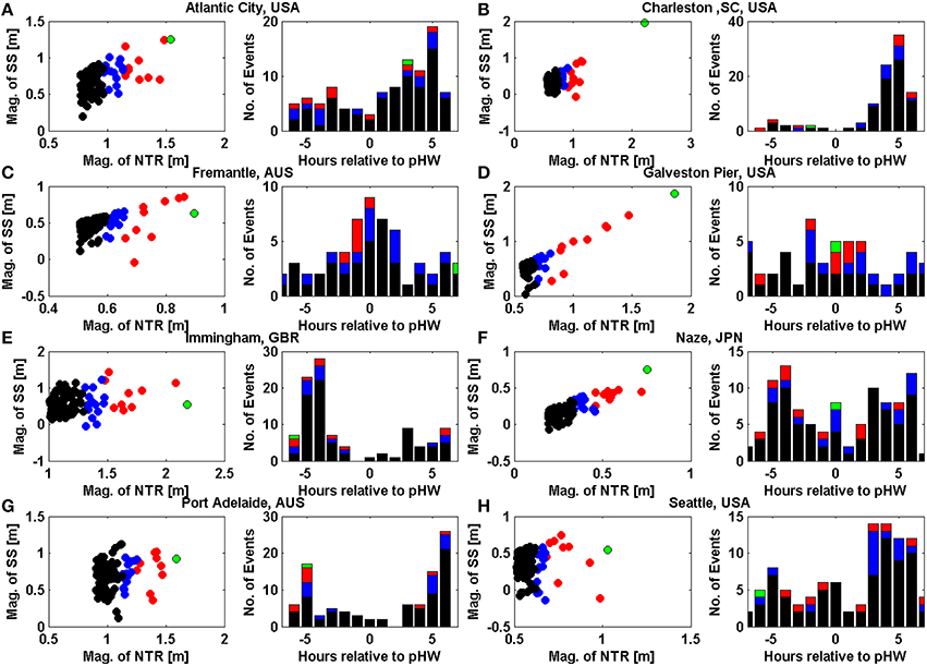
Figure 4. For eight selected sites: (A) Atlantic City, USA; (B) Charleston, USA; (C) Fremantle, Australia; (D) Galveston, USA; (E) Immingham, UK; (F) Naze, Japan; (G) Port Adelaide, Australia; (H) Seattle, USA. Left, scatter plot of 200 largest NTR and the associated skew surge value, right histogram of the time of the peak NTR relative to predicted high water. Both plots are cultured according to magnitude with green showing the maximum NTR, red the top 10 NTR and blue the top 25 NTR, black are the remainder of the top 200 NTR.
As mentioned earlier, tide-surge interaction has been most studied in the southern North Sea, where the largest positive NTR tend to occur on the rising tide and not at high water. This pattern can be clearly observed in the results for Immingham shown on Figure 4E. However, these distributions vary around the world. For example, at Fremantle in Australia (Figure 4C) tide-surge interaction appears to lead to most peaks in NTR occurring near the time of predicted HW. For Charleston (Figure 4B) and Seattle (Figure 4H) in USA, the majority of peaks in NTR occur on the ebb tide.
Skew Surge and Non-Tidal Residual Comparison
Our second objective was to determine if using skew surge to assess changes in storm surge activity, gave different results compared to using the NTR. As we identified in the section above, tide-surge interaction is evident at a large proportion of the study sites, suggesting that trends in skew surges and NTR may also differ. The trends calculated for the 95th, 99th, and 99.9th percentiles of the NTR are plotted in Figure 5, against the trends in skew surge time-series for the same three percentiles. Given the differences in sampling of the two parameter, as summarized in Section Methodology, comparisons of trends in different percentiles gives an understanding of how to relate the percentiles of the two parameters to each other. If the trends were the same between skew surge and NTR, all points would lie along the 1:1 ratio line shown on each figure. Trend differences between the skew surge and the NTR are generally small, with trends of the same percentiles of skew surge and NTR showing the closest comparison (i.e., the closest 1:1 match occurs between the 99th percentile of NTR and the 99th percentile of skew surge). The color of each dot in Figure 5 represents the height of MTR at that site. Sites with the largest difference between trends in skew surge and NTR typically have a large MTR. These sites include Broome, Australia, Ilfracombe, UK and Hoek van Holland, Netherlands, and these sites also have a large tide-surge interaction as quantified by the χ2 test statistics (Figures 3B,C). At three further sites, Calais, France, Darwin, Australia and Eastport, USA, the trend in skew surge is significantly larger than the trend in NTR (i.e., the 95% confidence intervals of the two trends do not overlap). The trends at Calais and Eastport change from significant negative trends (at the 95% level) to positive trends that are significant at the 66% level. The root mean squared error (RMSE) between skew surge trends and NTR trends are listed for each plot on Figure 5. The RMSEs are largest for the 99.9th percentile, since trends in this percentile can be affected by individual large events.
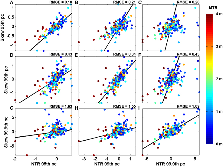
Figure 5. Scatter plots comparing trends in the 95th, 99th and 99.9th percentiles and NTR (labeled along the x-axis), to the same percentiles of skew surge (labeled along the y-axis). Each point is shaded according to the average mean tidal range at each site. The black line shows 1:1 ratio. The root mean squared error value for each plot is the value for the best fit (red line).
The time-series of the 99th (blue) and 99.9th (red) percentiles of skew surges are presented in Figure 6 for selected sites, along with the linear trends in these time-series and the corresponding 95% confidence intervals. The variability around the 99.9th percentile, which captures only the annual maximum of skew surge, is large relative to the magnitude of the linear trend and therefore very few significant trends can be detected. Therefore we use the 99th percentile of skew surge throughout the rest of the paper. Previous studies, including Menéndez and Woodworth (2010), used the 99th percentile of NTR, so our choice allows direct comparison with the results of that study.
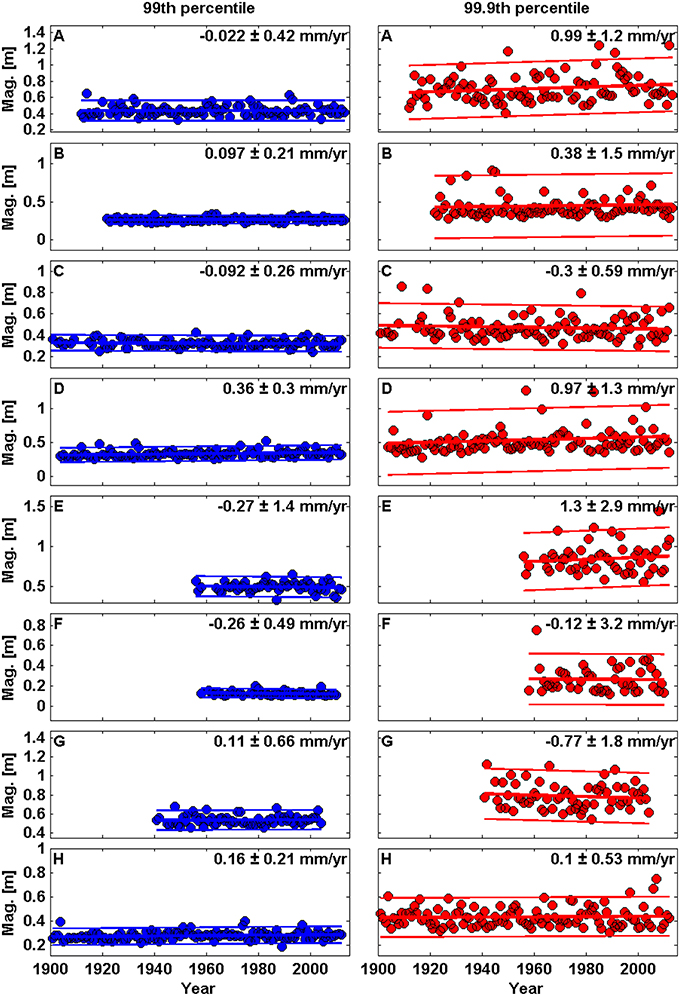
Figure 6. Time series plots of annual values of the 99th (blue) and 99.9th (red) percentile for skew surge at 8 selected sites. (A) Atlantic City, USA; (B) Charleston, USA; (C) Fremantle, Australia; (D) Galveston, USA; (E) Immingham, UK; (F) Naze, Japan; (G) Port Adelaide, Australia; (H) Seattle, USA.
Linear trends calculated for the 99th percentile of skew surge and NTR are shown for each site in Figures 7A,B respectively. Significant trends are shown with larger dots, with the color representing the magnitude of the trends. Overall there are few significant trends in skew surge time-series, with significant negative trends at 18 sites and significant positive trends at 11 sites. For the NTR there are significant negative trends at 33 sites and significant positive trends at only 5 sites. There are 15 sites with negative trends in both parameters, and 4 sites with positive trends in both. Trends were calculated at sites with enough years for the last 20, 40, 60, and 80 years, and compared to the trend of the entire time series. These results are presented in Supplementary Material and show that the number of positive and negative trends are roughly similar, and low in relation to the number of sites. Despite the low numbers of sites with significant trends there are some regions with consistent trends between neighboring stations, such as coherent decreases around north Australia and the Atlantic coast of southern Europe.
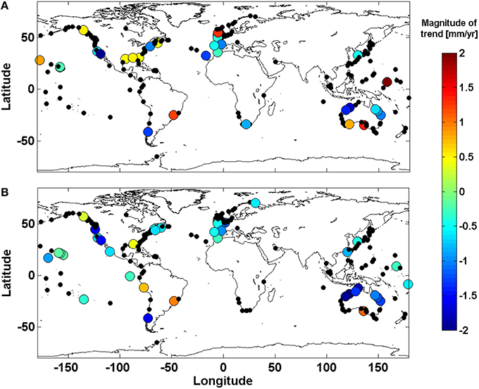
Figure 7. Shows the magnitude of the trend in in the 99th percentile of (A) skew surge and (B) NTR, for the 220 sites analyzed. Large dots show that the trend is significant at the 95% level.
Spatial Variability of Skew Surge
Our third objective is to assess the extent to which there is spatial coherence in skew surge variability, both locally (i.e., between adjacent tide gauge sites) and regionally (i.e., across ocean basins). For each site in turn, correlation coefficients were calculated between the unfiltered 99th percentile time series at that site and each of the other 219 sites. The results are shown in Figure 8. There are distinct regions where strong positive correlations occur among neighboring sites. These include the north-east Pacific, north-west Atlantic and sites in northern Europe. Interestingly, sites on the west coast of the US are weakly anti-correlated (at the 66% level) with several sites in northern Europe.
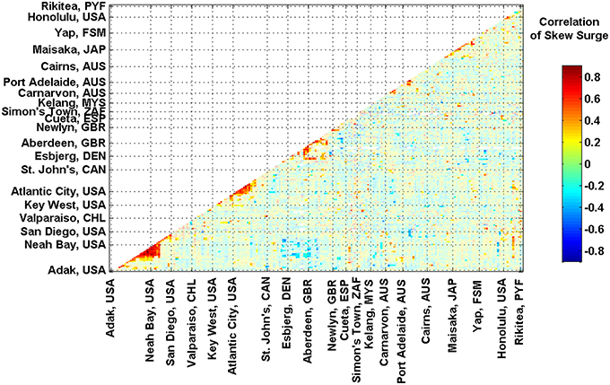
Figure 8. Correlation between each site. Each site is plotted along an imaginary coastline running from Alaska down the west and up the east coast of the America, across to the Atlantic to Norway, down through Europe around Africa, around the Indian Ocean, up the western Pacific Ocean and then across the Pacific Islands to the east. Sites with correlations at the 66% level are shown as bold color.
The strong correlation between groups of sites implies that we can create regional skew surge indices that represent the average skew surge conditions for a particular region; similar to what other studies have done for MSL (e.g., Shennan and Woodworth, 1992; Woodworth et al., 1999, 2009; Haigh et al., 2009a; Wahl et al., 2013; Dangendorf et al., 2014; Thompson and Mitchum, 2014). We identified 8 regions, where a large density of sites meant that strong positive correlations existed between them. These regions, and the sites of which they are comprised, are detailed in Table 1 and include the: north-east Pacific (NEP), Gulf of Mexico (GOM), north-west Atlantic South (NWA-S), north-west Atlantic North (NWA-N), North Sea (NS), west Australia (WAUS), east Australia (EAUS), and Japan (JAP).
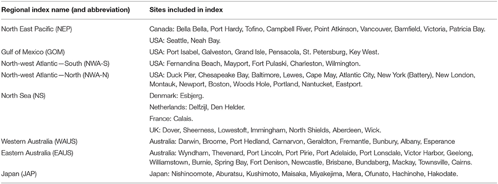
Table 1. Details of sites included in each of the regional indices.
An example of the creation of a regional index is shown in Figure 9 for the north-east Pacific. The de-trended, normalized time-series from each of the 11 selected sites in the region are plotted in Figure 9A, with an arbitrary offset. These time series are overlaid in Figure 9B. The thicker red lines shows the regional time-series that has been created by averaging the de-trended, normalized time-series for each of the 11 sites. The locations of the 11 sites used to calculate the regional index are shown in Figure 9C, as red dots. Similar figures for the other 8 regions are shown in the Supplementary Material.
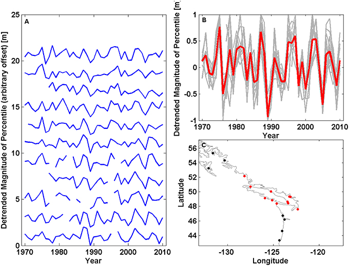
Figure 9. Creation of regional skew surge index for the north-east Pacific. (A) The de-trended time series of the 99th percentile for each site from north to south (see Table 1 for site ID), (B) All the time-series with the mean of all sites plotted in red, and (C) the sites that are in this region highlighted in red.
There is considerable year-to-year variability in the 8 regional indices. To better investigate the inter-decadal variability we applied a Loess filter to each of the 8 regional skew surge indices, and the filtered time series are shown in Figure 10A. Concurrent peaks in skew surge are observed in multiple regions, most notably in 1992–1993 in the north-west Atlantic (North and South indices) and the North Sea. Peaks in skew surge in the southern North Atlantic throughout the 1990s appear to lag peaks in the Gulf of Mexico by approximately 1 year. Storm seasons for these regions are summer and winter respectively and the lag may be a result of this or a delay in the response to changes in regional scale climatology.
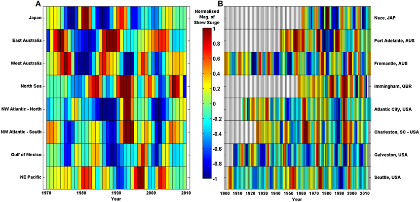
Figure 10. Temporal variability of 8 selected regions as shown by the de-trended normalized and then filtered magnitude of skew surge for: (A) regional indices; (B) selected long site from each region, which has a strong correlation with the regional index.
The 8 regional skew surge indices are plotted as stacked time series in Figure 11A, with the correlations between them shown in Figure 11B. Between many regions, there is a strong correlation (r > 0.5), but at the 95% level these are not significant, due largely to the reduction in the number of effective observations when autocorrelation is accounted for. Strong correlations exist between: the two north-west Atlantic indices (r = 0.65, p = 0.02), the Gulf of Mexico and both two north-west Atlantic indices (South: r = 0.37, p = 0.33; North: r = 0.31, p = 0.4), the North Sea and north-west Atlantic—South (r = 0.65, p = 0.12). Therefore, only this last correlation is significant at the 80% level.
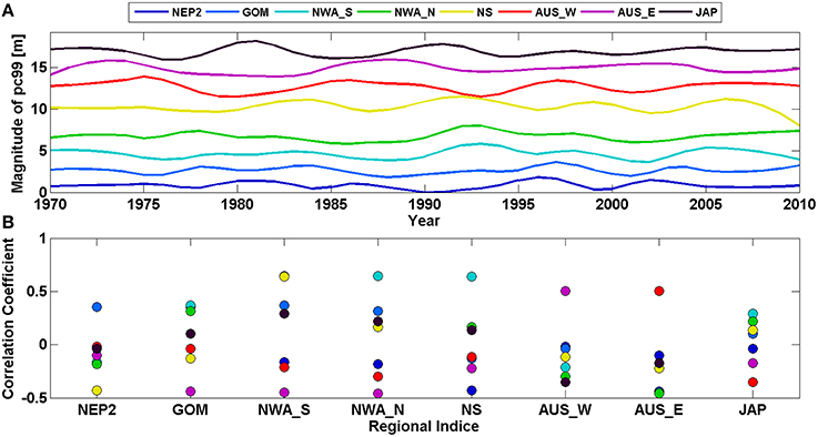
Figure 11. (A) Stacked time series of filtered regional skew surge indices, with arbitrary offset applied, (B) Correlation of each filtered regional skew surge index against the others.
The regional skew surge indices were only calculated for the period 1970–2010, because fewer sites with valid data outside of this period increases the variability in the indices. To allow longer temporal comparisons between regions, we selected individual sites within each region that were both long and highly correlated with the regional index. The 8 sites with long records, across the 8 regions, are shown in Figure 10B. Note, these time series have also be subjected to the same Loess filter, applied to the regional time series. The simultaneous peak in the 1990s, mentioned above, is also present in the individual sites. However, a peak in the signal in the filtered time series at Charleston and Atlantic City, USA in the 1960s is not clear at Immingham, UK. The reverse is true in the late 1980s, where an increase at Immingham is not present at Charleston or Atlantic City.
Comparison of Skew Surge to Climate Indices
Our fourth objective is to compare inter-annual and multi-decadal variations in skew surge with fluctuations in regional climate. Correlation coefficients were calculated between the 8 regional skew surge indices and each of the 8 regional climate indices. The results are shown in Figure 12.
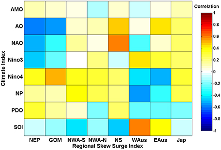
Figure 12. Correlation of regional indices of skew surge against key climatic indices.
There are no statistically significant correlations at the 95% level, again largely because of the large degree of autocorrelation in the filtered time-series. Strong positive correlations (r > 0.5) occur between: the North Sea and NAO (r = 0.60, p = 0.28), the Gulf of Mexico and Nińo 4 (r = 0.52, p = 0.19) and western Australian and SOI (r = 0.59, p = 0.31). Strong negative correlations (r < −0.5) occur between the north-east Pacific and AO (r = −0.57, p = 0.28) and NAO (r = −0.50, p = 0.40), the Gulf of Mexico and AO (r = −0.53, p = 0.32), western Australia and NP (r = −0.56, p = 0.28), and eastern Australia and Nińo 4 (r = −0.52, p = 0.19). The correlations detailed above that involve Nińo 4 are the only correlations significant at the 80% level.
The peak observed in the north-east Pacific index in 1997–1998 (Figure 10A), corresponds to one of the strongest El Nińo events in the time-series. The peak observed in both the Seattle record and the NEP index in 1982–1983 corresponds to another strong El Nińo event, however, the El Nińo event of 1972 is not evident in the skew surge time series. Also, the typically positive Nińo 3 values observed through the early 1990s coincide with a trough in the north-east Pacific index. The presence of a peak in north-east Pacific index during only the strongest El Nińo events suggest a complex relationship between skew surge and the magnitude of variability in regional climate.
Discussion
One of the key goals of this paper was to determine if different results are obtained when using skew surge to assess changes in storm surge activity, compared to the more traditional NTR. As Horsburgh and Wilson (2007) showed, while the NTR primarily contains the meteorological contribution termed the surge, it may also contain harmonic prediction errors or timing errors, and non-linear interactions, which can bias analysis of storm surges. It is for this reason that we wanted to assess the alternative use of skew surges. The advantage of using skew surge is that it is an integrated and unambiguous measure of the storm surge (Haigh et al., 2015). Changes in skew surges have only previously been assessed (to our knowledge) at sites around the north-west Europe (Batstone et al., 2013; Dangendorf et al., 2014) and the USA (Wahl and Chambers, 2015). Both of these regions generally display semi-diurnal tidal behavior, but our method works well in all tidal regimes.
We found that significant tide-surge interaction occurs at 130 of the 220 sites analyzed (59%) based on the tidal-level method, and 175 sites (81%) based on tidal-phase approach. These sites include those previously reported, as well as regions not previously identified in the literature, such as the Gulf of Panama and the Malay Peninsula. We also found that tide-surge interaction is not limited to locations with large adjacent areas of shallow bathymetry. Smaller but still statistically significant interactions occur along the Pacific coast of North America, on a number of Pacific Islands and around the Iberian Peninsula. The topography of these sites is highly variable. Some sites are in shallow water such as Willapa Bay, USA, which is in a large bay, and Astoria, USA, which is influenced by the Columbia River. Other sites are on volcanic islands rising steeply from the ocean floor, such as Papette, French Polynesia and Pohnpei, the Federated States of Micronesia. For both these island sites there is an increased frequency of peaks in NTR around the time of predicted HW, a pattern that is also observed at Galveston, USA (Figure 4D).
In some regions the timing of the peak NTR relative to tidal-phase, and therefore the level of tide-surge interaction is site specific. For example, around the UK, peak NTR usually occurs away from predicted HW (Horsburgh and Wilson, 2007; Haigh et al., 2010; Olbert et al., 2013), and in the North Sea Horsburgh and Wilson (2007) showed that the external surge component will always peak away from predicted HW. However, at Larne and Bangor in Northern Ireland, peak NTR most frequently occurred at predicted HW (Olbert et al., 2013). These sites have similar tidal conditions and are geographically close but highlight that small changes in bathymetry and tidal range can influence the extent of tide-surge interaction.
Individual storm characteristics vary from the average pattern, and where these deviations occur in the largest storm surges the difference in skew surge magnitude can be important. At Wake Island in the Pacific, Typhoon Ioke generated a NTR of 1.5 m but a skew surge of only 1.0 m, because the peak NTR for this event occurred 5 h before predicted HW (see Figure A3.10 in Supplementary Material, Site 434). However, no significant tide-surge interaction is observed at this site and the peak NTR for an event like Typhoon Ioke could have occurred at predicted HW. Conversely, at Brest, France, where significant tide-surge interaction meant that peaks in NTR usually occurred away from predicted HW, the maximum NTR (caused by the so-called Great Storm in October 1987) occurs at the same time as predicted HW. Therefore, although the skew surge is a more reliable indicator of the average meteorological influence on sea level, individual storm surges may have different characteristics. Parameterization of any physical process aims to use one value to represent a complex system, and this must be considered when we use skew surge in ESL calculations. This is especially true in regions with small tidal ranges or those affected by tropical cyclones. The rapid peak in storm surge associated with tropical cyclones reduces the influence of storm surge on tidal propagation, and may lead to a more uniform distribution of peak NTR timing relative to predicted HW.
Although tide-surge interaction is evident at many sites, and there are differences between skew surge and NTR values, we found that at most sites, the trends in skew surge are very similar to those in NTR. The largest differences in trends are at sites along the north-coast of Australia or the French coast of the English Channel, and this results in the reversal of trends at Calais and Darwin. Both locations have macro-tidal regimes with significant tide-surge interaction. The general similarity in trends means we can compare our results to previous studies which used NTR. Menéndez and Woodworth (2010) found more negative trends in NTR than positive trends globally. We also find more negative trends in NTR, but no statistically significant difference between the number of positive and negative trends in skew surge time-series. Our findings are consistent with those of Wahl and Chambers (2015) for the US, who found a greater number of sites had significant trends in NTR compared to skew surge. The number of sites with significant trends in skew surge and NTR may be generated from chance, but a formal assessment has not been made here, because of the spatially non-homogenous dataset. Methods such as that of Livezey and Chen (1983) could be adapted to assess whether the number of trends is statistically significant. Even so, there are a greater number of negative trends in NTR than skew surge and this may be caused by timing errors or changes in the tide-surge interaction. Timing errors are particular evident in early records that have been digitized from paper charts and are often associated with issues with the older mechanical tide gauges (Pugh and Woodworth, 2014). Therefore, timing errors are more prevalent in the early part of the tide gauge records, and if they are included in the analysis they may introduce a negative bias into the NTR time-series. By definition, time-series of skew surges are not influenced by such timing errors. Another possible reason for the difference in trends is that the magnitude of the tide-surge interaction is changing through time, because of changes in the phase or magnitude of the tide (e.g., Mawdsley et al., 2015). Previous studies in the North Sea (Horsburgh and Wilson, 2007) and English Channel (Haigh et al., 2010) however, found no significant changes in tide-surge interaction over time. We have not investigated this, in this study.
We found little spatial coherence in the magnitude and sign of trends among sites, mainly because the trends are insignificant at most sites. However, in northern Australia a number of sites display significant negative trends in skew surge (Figure 7) and in NTR, which is consistent with Menéndez and Woodworth (2010), while our findings also support their research showing positive trends at sites in the Gulf of Mexico and along the Atlantic coast of Florida. However, most other findings vary from those of Menéndez and Woodworth (2010). We find a decrease at sites in southern Europe, and an increase at a number of sites in southern Australia. No coherent trend along the north-east coast of America is observed in this study, which agrees with Zhang et al. (2000) but contradicts the increase found in this region by both Menéndez and Woodworth (2010) and Grinsted et al. (2012). Differences between our findings and those of Menéndez and Woodworth (2010) may be the result of further quality control, or the inclusion of new data, which along the north-east coast of America included large storms surges in 2010 and 2012, generated by Hurricanes Irene and Sandy, respectively. Figures A3.1–3.4, in the Supplementary Material, show that trends over the last 20–80 years change depending on the period studied, and therefore extra data can change results. In other studies of ESL, changes may also be caused by the inclusion of tide, such as the increases in New York (Talke et al., 2014), western Northern America (Bromirski et al., 2003; Abeysirigunawardena and Walker, 2008; Cayan et al., 2008) and the German Bight (Müdersbach et al., 2013). Mawdsley et al. (2015) observed significant increases in tidal HW in all these regions, and we speculate that this has contributed toward the observed increase in ESL, in other studies, and the lack of trends in skew surges identified by this paper in these areas. With the growing literature regarding changes in tide (e.g., Jay, 2009; Woodworth, 2010; Pickering et al., 2012; Pelling et al., 2013; Mawdsley et al., 2015), it is essential that studies of storm surge use parameters that just relate to meteorological changes and identify other drivers of change, such as the tide or tide-surge interaction.
The number of statistically significant trends is low, in part, because of the large inter-annual variability in the high percentiles of skew surges. The creation of filtered regional skew surge indices removed the high frequency variability and helped to reveal underlying inter-decadal variability and the spatial coherence between regional signals. However, despite strong correlations between some regions around the North American coastline and across the Atlantic to the North Sea, none of the correlations are significant at the 95% level. Just prior to completing our study, we learnt of a similar investigation by Marcos et al. (2015). Using the GESLA dataset, they showed that the intensity and frequency of ESL unrelated to MSL display a regional coherence on decadal time-scales. Their finding points toward large-scale climate drivers of decadal changes in storminess (Marcos et al., 2015). The string correlations between neighboring sites show that these large scale climatic drivers are important, but there significance is difficult to assess in relatively short datasets have a high degree of temporal auto-correlation.
Comparisons of regional storm surge time-series and climate indices have been undertaken in numerous past studies. Menéndez and Woodworth (2010) found the Nińo 3 index had a positive correlation with the magnitude of NTR in the eastern Pacific and a negative correlation in the western equatorial Pacific. The magnitude of an El Nińo appears to influence the north-east Pacific index, with peaks in the index associated with the largest El Nińo events in 1982–1983 and 1997–1998, but a trough in the index during small but positive values of the Nińo 3 index in the early 1990s. Also in the Pacific the PDO was previously shown to correlate positively with sites in the northeast Pacific (Abeysirigunawardena and Walker, 2008), however we do not find any significant correlation. The findings related to the North Sea index supports previous studies (e.g., Haigh et al., 2010) that find a positive correlation with the NAO, although our correlation is not significant. Studies by Ezer and Atkinson (2014) and Talke et al. (2014) found anti-correlation between the NAO and sites on the US east coast, but we find very weak (and non-significant) correlations. Our method of using filtered regional skew surge indices, means that although strong correlations (r > 0.5) are observed between some regional skew surge indices and climate indices, they are not deemed significant at the 95% level. The effect of autocorrelation in the calculation reduces the degrees of freedom (effective observations) from 40 to less than 8 for all correlation calculations, and therefore increases the size of the confidence intervals. The significance of correlations may improve with increased data length or reduced filter size, however, filters are a widely used and during the development of the methodology the 10 year Loess filter was found to give the lowest RMSE. In this study we have correlated skew surge time-series against climate indices, but it would be more appropriate to use wind and pressure datasets, as these are the parameters that directly cause storm surges. In the future, we hope to do this using meteorological re-analysis datasets, like Bromirski et al. (2003), Calafat et al. (2013) and Wahl and Chambers (2015) did to assess storm surge variability in their regional studies.
One of the main limitations of this study (and other studies) remains the relatively small number of sites and the limited length of the time-series available. Although the GESLA dataset is probably the most comprehensive collection of hourly sea level data, there are still many under-represented regions in the database. The 8 regional indices we derived all cover data dense regions since this is where the strongest correlations are, but even here the number of datasets longer than 40 years limited the length of the regional skew surge indices. The application of the filter, which is necessary to extract relationships between the datasets, meant that the confidence intervals increased and the significance of the correlations decreased. There is a need for either more sites or better access to data in under-represented areas, especially areas that are prone to large storm surges, such as the Caribbean, the Bay of Bengal and countries around the South China Sea. Conversely, the already global nature of the study does not allow for a detailed understanding of the findings presented here. Further work conducted on a local to regional scale, should be undertaken to assess the mechanisms that are driving the tide-surge interaction, and control its specific signature. Such assessment could consider differences in the tide-surge interaction for tropical and extra-tropical storms, the influence of slope angle or shelf width, or the effect of changes in bathymetry.
Conclusions
In this paper, we have used time series of skew surge to assess changes in storm surges on a quasi-global scale for the first time. Past studies that have assessed changes in storm surges have tended to focus on the NTR, which includes contributions from non-meteorological generated factors, which may bias results. This study also assessed the spatial and temporal variability in the skew surge, using regional indices.
First, we determined the extent of tide-surge interaction, at each of the 220 study sites, as this determines the scale of the differences between skew surge and NTR values. Using χ2 test statistics we found statistically significant (95% confidence) levels of tide-surge interaction at 130 of the 220 sites (59%) based on tidal-level and 175 sites (81%) based on tidal-phase. The tide-surge interaction is strongest in regions of shallow bathymetry such as the North Sea, north Australia and the Malay Peninsula. However, non-standard distributions are also observed at sites on open ocean islands, although at these sites the peak in NTR often tended toward the time of predicted HW, rather than away from it as experienced in shallow water areas (such as the North Sea).
Second, we determined if different results are obtained when using skew surges to assess changes in storm surge activity, compared to the more traditional NTR. At most sites the trends in skew surge are similar to those of NTRs. Where the differences in trends were large, the sites tended to have a large tidal range, such as those in northern Australia and northern France. Although at most sites the trends in skew surges were not statistically significant, we observed approximately equal numbers of positive and negative trends. However, there were more negative trends in the NTR. This suggests that skew surge improves the calculation of trends, because phase offsets caused by time errors are not present in time series of skew surges.
Third, we examined the extent to which there is spatial coherence in skew surge variability, both locally (i.e., among adjacent tide gauge sites) and regionally (i.e., across ocean basins). We identified 8 regions, where there were strong positive correlations among neighboring sites, and hence derived a regional index for each region. We observed a number of strong (r > 0.5) correlations between regions, including: positive correlation between the two regions on North American Atlantic coast, positive correlation between the north-west Atlantic—south and the North Sea; and negative correlation between the North Sea and north-east Pacific. However, these trends were not significant at the 95% level, since the high degree of autocorrelation in the filtered dataset increased the size of the confidence intervals.
Finally, we compared multi-decadal variations in skew surge with fluctuations in regional climate. Again strong correlations were observed, but were not significant at the 95% level. Correlations significant at the 80% level included those between the Gulf of Mexico and eastern Australia and the Nińo 4 index.
Author Contributions
RM conducting the data quality control for all tide gauge sites, before developing and coding the method for extraction of the skew surge. Also was primarily involved in creation of Figures and writing of text. IH developed and coded some of the method for skew surge extraction, as well as the chi-squared test to assess tide-surge interaction. Also heavily involved with editing of text.
Conflict of Interest Statement
The authors declare that the research was conducted in the absence of any commercial or financial relationships that could be construed as a potential conflict of interest.
Acknowledgments
This study was funded by the University of Southampton, School of Ocean and Earth Science and the National Environmental Research Council (NERC). Conversations and feedback from Phillip Woodworth, Neil Wells and Francisco Calafat at the National Oceanography Centre have been invaluable. We thank the reviewers of the paper, whose excellent comments have improved this paper. The GESLA data set was initially collated by staff from the National Oceanography Centre (NOC), Liverpool in the UK and the Antarctic Climate and Ecosystems Cooperative Research Centre (ACE CRC) in Australia. Extensions to the dataset were provided by: University of Hawaii Sea Level Center (UHSLC), National Oceanographic and Atmospheric Authority (NOAA), British Oceanographic Data Centre (BODC), Norwegian Mapping Authority (NMA), Marine Environmental Data Service (MEDS); Bureau of Meteorology (BOM); and Norwegian Mapping Authority (NMA). This paper contributes to the Engineering and Physical Science Research Council Flood Memory Project (grant number EP/K013513/1).
Supplementary Material
The Supplementary Material for this article can be found online at: http://journal.frontiersin.org/article/10.3389/fmars.2016.00029
References
Abeysirigunawardena, D. S., and Walker, I. J. (2008). Sea level responses to climatic variability and change in Northern British Columbia. Atmosp. Ocean 46, 277–296. doi: 10.3137/ao.460301
Antony, C., and Unnikrishnan, A. S. (2013). Observed characteristics of tide-surge interaction along the east coast of India and the head of Bay of Bengal. Estuarine Coast. Shelf Sci. 131, 6–11. doi: 10.1016/j.ecss.2013.08.004
Araújo, I. B., and Pugh, D. T. (2008). Sea levels at Newlyn 1915–2005: analysis of trends for future flooding risks. J. Coastal Res. 24, 203–212. doi: 10.2112/06-0785.1
Batstone, C., Lawless, M., Tawn, J., Horsburgh, K., Blackman, D., McMillan, A., et al. (2013). A UK best-practice approach for extreme sea-level analysis along complex topographic coastlines. Ocean Eng. 71, 28–39. doi: 10.1016/j.oceaneng.2013.02.003
Bell, G. D., and Chelliah, M. (2006). Leading tropical modes associated with interannual and multidecadal fluctuations in North Atlantic hurricane activity. J. Clim. 19, 590–612. doi: 10.1175/JCLI3659.1
Bernier, N., and Thompson, K. (2007). Tide-surge interaction off the east coast of Canada and northeastern United States. J. Geophys. Res. 112, C06008. doi: 10.1029/2006jc003793
Box, G. E. P., Jenkins, G. M., and Reinsel, G. C. (1994). Time Series Analysis: Forecasting and Control. 3rd Edn. Upper Saddle River, NJ: Prentice-Hall.
Bromirski, P. D., Flick, R. E., and Cayan, D. R. (2003). Storminess variability along the California Coast: 1858–2000. J. Clim. 16, 982–993. doi: 10.1175/1520-0442(2003)016<0982:SVATCC>2.0.CO;2
Calafat, F. M., Chambers, D. P., and Tsimplis, M. N. (2013). Inter-annual to decadal sea-level variability in the coastal zones of the Norwegian and Siberian Seas: the role of atmospheric forcing. J. Geophys. Res. 118, 1287–1301. doi: 10.1002/jgrc.20106
Cayan, D. R., Bromirski, P. D., Hayhoe, K., Tyree, M., Dettinger, M. D., and Flick, R. E. (2008). Climate change projections of sea level extremes along the California coast. Clim. Change 87, S57–S73. doi: 10.1007/s10584-007-9376-7
Church, J. A., Clark, P. U., Cazenave, A., Gregory, J. M., Jevrejeva, S., Levermann, A., et al. (2013). “Sea level change,” in Climate Change 2013: The Physical Science Basis. Contribution of Working Group I to the Fifth Assessment Report of the Intergovernmental Panel on Climate Change, eds T. F. Stocker, D. Qin, G.-K. Plattner, M. Tignor, S. K. Allen, J. Boschung, A. Nauels, Y. Xia, V. Bex, and P. M. Midgley (Cambridge, UK; New York, NY: Cambridge University Press), 1137–1216.
Cleveland, W. S., and Devlin, S. J. (1988). Locally weighted regression: an approach to regression analysis by local fitting. J. Am. Stat. Assoc. 83, 596–610. doi: 10.1080/01621459.1988.10478639
Dangendorf, S., Calafat, F. M., Arns, A., Wahl, T., Haigh, I. D., and Jensen, J. (2014). Mean sea level variability in the North Sea: processes and implications. J. Geophys. Res. 119, 6820–6841. doi: 10.1002/2014jc009901
Dixon, M. J., and Tawn, J. A. (1994). Extreme Sea-Levels at the UK A-Class Sites: Site-by-Site Analyses. Proudman Oceanographic Laboratory, Internal Document, No. 65, 229.
Emanuel, K. A., Sundararajan, R., and Williams, J. (2008). Hurricanes and global warming: results from downscaling IPCC AR4 simulations. Bull. Am. Meteorol. Soc. 89, 346–367. doi: 10.1175/bams-89-3-347
Ezer, T., and Atkinson, L. P. (2014). Accelerated flooding along the U.S. East Coast: on the impact of sea-level rise, tides, storms, the Gulf Stream, and the North Atlantic Oscillations. Earth Fut. 2, 362–382. doi: 10.1002/2014EF000252
Feng, X., and Tsimplis, M. N. (2014). Sea level extremes at the coasts of China. J. Geophys. Res. 119, 1593–1608. doi: 10.1002/2013jc009607
Grinsted, A., Moore, J. C., and Jevrejeva, S. (2012). Homogeneous record of Atlantic hurricane surge threat since 1923. Proc. Natl. Acad. Sci. U.S.A. 109, 19601–19605. doi: 10.1073/pnas.1209542109
Haigh, I., Nicholls, R., and Wells, N. (2009a). Mean sea level trends around the English Channel over the 20th century and their wider context. Cont. Shelf Res. 29, 2083–2098. doi: 10.1016/j.csr.2009.07.013
Haigh, I., Nicholls, R., and Wells, N. (2009b). Twentieth-Century changes in extreme still sea levels in the English channel. Coast. Eng. 2008. 1–5, 1199–1209. doi: 10.1142/9789814277426_0100
Haigh, I., Nicholls, R., and Wells, N. (2010). Assessing changes in extreme sea levels: Application to the English Channel, 1900–2006. Cont. Shelf Res. 30, 1042–1055. doi: 10.1016/j.csr.2010.02.002
Haigh, I., Wijeratne, E. M. S., MacPherson, L., Pattiaratchi, C., Mason, M., Crompton, R., et al. (2014). Estimating present day extreme water level exceedance probabilities around the coastline of Australia: tides, extra-tropical storm surges and mean sea level. Clim. Dynam. 42, 121–138. doi: 10.1007/s00382-012-1652-1
Haigh, I. D., Wadey, M. P., Gallop, S. L., Loehr, H., Nicholls, R. J., Horsburgh, K., et al. (2015). A user-friendly database of coastal flooding in the United Kingdom from 1915–2014. [Data Descriptor]. Sci. Data 2, 150021. doi: 10.1038/sdata.2015.21
Hartmann, D. L., Klein Tank, A., and Rusticucci, M. (2013). “Observations: ocean,” in Climate Chanage 2013: The Physical Scientific Basis. Working Group I Contribution to the Intergovernmental Panel on Climate Change 5th Assessment Report, eds J. Hurrell, J. Marengo, F. Tangang, and P. Viterbo (Cambridge, UK; New York, NY: Cambridge University Press), 159–254.
Horsburgh, K. J., and Wilson, C. (2007). Tide-surge interaction and its role in the distribution of surge residuals in the North Sea. J. Geophys. Res. 112, C08003. doi: 10.1029/2006jc004033
Hunter, J. (2012). A simple technique for estimating an allowance for uncertain sea-level rise. Clim. Change 113, 239–252. doi: 10.1007/s10584-011-0332-1
Hunter, J. R., Church, J. A., White, N. J., and Zhang, X. (2013). Towards a global regionally varying allowance for sea-level rise. Ocean Eng. 71, 17–27. doi: 10.1016/j.oceaneng.2012.12.041
Idier, D., Dumas, F., and Muller, H. (2012). Tide-surge interaction in the English Channel. Nat. Hazards Earth Syst. Sci. 12, 3709–3718. doi: 10.5194/nhess-12-3709-2012
Jay, D. A. (2009). Evolution of tidal amplitudes in the eastern Pacific Ocean. Geophys. Res. Lett. 36, L04603. doi: 10.1029/2008gl036185
Kossin, J. P., Knapp, K. R., Vimont, D. J., Murnane, R. J., and Harper, B. A. (2007). A globally consistent reanalysis of hurricane variability and trends. Geophys. Res. Lett. 34:L04815. doi: 10.1029/2006gl028836
Lionello, P., Mufato, R., and Tomasin, A. (2005). Sensitivity of free and forced oscillations of the Adriatic Sea to sea level rise. Clim. Res. 29, 23–39. doi: 10.3354/cr029023
Livezey, R. E., and Chen, W. Y. (1983). Statistical field significance and its determination by monte carlo techniques. Mon. Weather Rev. 111, 46–59. doi: 10.1175/1520-0493(1983)111<0046:sfsaid>2.0.co;2
Marcos, M., Calafat, F. M., Berihuete, Á., and Dangendorf, S. (2015). Long-term variations in global sea level extremes. J. Geophys. Res. 120, 8115–8134. doi: 10.1002/2015jc011173
Marcos, M., Tsimplis, M. N., and Shaw, A. G. P. (2009). Sea level extremes in southern Europe. J. Geophys. Res. 114:C01007. doi: 10.1029/2008JC004912
Mawdsley, R. J., Haigh, I. D., and Wells, N. C. (2015). Global secular changes in different tidal high water, low water and range levels. Earth Fut. 3, 66–81. doi: 10.1002/2014EF000282
Menéndez, M., and Woodworth, P. L. (2010). Changes in extreme high water levels based on a quasi-global tide-gauge data set. J. Geophys. Res. 115, C10011. doi: 10.1029/2009JC005997
Müdersbach, C., Wahl, T., Haigh, I. D., and Jensen, J. (2013). Trends in high sea levels of German North Sea gauges compared to regional mean sea level changes. Cont. Shelf Res. 65, 111–120. doi: 10.1016/j.csr.2013.06.016
Olbert, A. I., Nash, S., Cunnane, C., and Hartnett, M. (2013). Tide–surge interactions and their effects on total sea levels in Irish coastal waters. [journal article]. Ocean Dynam. 63, 599–614. doi: 10.1007/s10236-013-0618-0
Pelling, H. E., Mattias Green, J. A., and Ward, S. L. (2013). Modelling tides and sea-level rise: to flood or not to flood. Ocean Modell. 63, 21–29. doi: 10.1016/j.ocemod.2012.12.004
Pickering, M. D., Wells, N. C., Horsburgh, K. J., and Green, J. A. M. (2012). The impact of future sea-level rise on the European Shelf tides. Cont. Shelf Res. 35, 1–15. doi: 10.1016/j.csr.2011.11.011
Pugh, D., and Woodworth, P. (2014). Sea-level Science: Understanding Tides, Surges, Tsunamis and Mean Sea-level Changes: Cambridge University Press.
Raicich, F. (2003). Recent evolution of sea-level extremes at Trieste (Northern Adriatic). Cont. Shelf Res. 23, 225–235. doi: 10.1016/S0278-4343(02)00224-8
Ray, R. D. (2009). Secular changes in the solar semidiurnal tide of the western North Atlantic Ocean. Geophys. Res. Lett., 36, L19601. doi: 10.1029/2009gl040217
Seneviratne, S. I., Nicholls, N., Easterling, D., Goodess, C. M., Kanae, S., Kossin, J., et al. (2012). “Changes in climate extremes and their impacts on the natural physical environment,” in Managing the Risks of Extreme Events and Disasters to Advance Climate Change Adaptation. A Special Report of Working Groups I and II of the Intergovernmental Panel on Climate Change (IPCC), eds C. B. Field, V. Barros, T. F. Stocker, D. Qin, D. J. Dokken, K. L. Ebi, et al. (Cambridge; New York, NY: Cambridge University Press), 109–230.
Shennan, I., and Woodworth, P. L. (1992). A comparison of late Holocene and twentieth-century sea-level trends from the UK and North Sea region. Geophys. J. Intern. 109, 96–105. doi: 10.1111/j.1365-246X.1992.tb00081.x
Talke, S. A., Orton, P., and Jay, D. A. (2014). Increasing storm tides in New York Harbor, 1844–2013. Geophys. Res. Lett. 41, 3149–3155. doi: 10.1002/2014GL059574
Thompson, P. R., and Mitchum, G. T. (2014). Coherent sea level variability on the North Atlantic western boundary. J. Geophys. Res. 119, 5676–5689. doi: 10.1002/2014jc009999
Thompson, P. R., Mitchum, G. T., Vonesch, C., and Li, J. (2013). Variability of Winter Storminess in the Eastern United States during the Twentieth Century from Tide Gauges. J. Clim. 26, 9713–9726. doi: 10.1175/JCLI-D-12-00561.1
Torres, R. R., and Tsimplis, M. N. (2013). Sea-level trends and interannual variability in the Caribbean Sea. J. Geophys. Res. 118, 2934–2947. doi: 10.1002/jgrc.20229
Trenberth, K. E., Jones, P. D., Ambenje, P., Bojariu, R., Easterling, D., Klein Tank, A., et al. (2007). “Observations: surface and atmospheric climate change,” in Climate Change 2007: The Physical Science Basis. Contribution of Working Group I to the Fourth Assessment Report of the Intergovernmental Panel on Climate Change, eds S. Solomon, D. Qin, M. Manning, Z. Chen, M. Marquis, K.B. Averyt, M. Tignor, and H. L. Miller (Cambridge; New York, NY: Cambridge University Press), 235–336.
Ullmann, A., Pirazzoli, P. A., and Tomasin, A. (2007). Sea surges in Camargue: trends over the 20th century. Cont. Shelf Res. 27, 922–934. doi: 10.1016/j.csr.2006.12.001
Valle-Levinson, A., Olabarrieta, M., and Valle, A. (2013). Semidiurnal perturbations to the surge of Hurricane Sandy. Geophys. Res. Lett. 40, 2211–2217. doi: 10.1002/grl.50461
Vecchi, G. A., and Soden, B. J. (2007). Increased tropical Atlantic wind shear in model projections of global warming. Geophys. Res. Lett. 34:L08702. doi: 10.1029/2006gl028905
von Storch, H., and Woth, K. (2008). Storm surges: perspectives and options. Sustainab. Sci. 3, 33–43. doi: 10.1007/s11625-008-0044-2
Wahl, T., and Chambers, D. P. (2015). Evidence for multidecadal variability in US extreme sea level records. J. Geophys. Res. 120, 1527–1544. doi: 10.1002/2014jc010443
Wahl, T., and Chambers, D. P. (2016). Climate controls multidecadal variability in U. S. extreme sea level records. J. Geophys. Res. 121. doi: 10.1002/2015JC011057
Wahl, T., Haigh, I. D., Woodworth, P. L., Albrecht, F., Dillingh, D., Jensen, J., et al. (2013). Observed mean sea level changes around the North Sea coastline from 1800 to present. Earth Sci. Rev. 124, 51–67. doi: 10.1016/j.earscirev.2013.05.003
Wolf, J. (1981). “Surge-tide interaction in the North Sea and River Thames,” in Floods Due to High Winds and Tides, ed D. H. Peregrine (New York, NY: Elseiver), 75–94.
Wong, P. P., Losada, I. J., Gattuso, J. P., Hinkel, J., Khattabi, A., McInnes, K. L., et al. (2014). “Coastal systems and low-lying areas,” in Climate Change 2014: Impacts, Adaptation, and Vulnerability. Part A: Global and Sectoral Aspects. Contribution of Working Group II to the Fifth Assessment Report of the Intergovernmental Panel of Climate Change, eds C. B. Field, V. R. Barros, D. J. Dokken, K. J. Mach, M. D. Mastrandrea, T. E. Bilir, et al. (Cambridge; New York, NY: Cambridge University Press), 361–409.
Woodworth, P. L. (2010). A survey of recent changes in the main components of the ocean tide. Cont. Shelf Res. 30, 1680–1691. doi: 10.1016/j.csr.2010.07.002
Woodworth, P. L., and Blackman, D. L. (2004). Evidence for systematic changes in extreme high waters since the mid-1970s. J. Clim. 17, 1190–1197. doi: 10.1175/1520-0442(2004)017<1190:EFSCIE>2.0.CO;2
Woodworth, P. L., and Menéndez, M. (2015). Changes in the mesoscale variability and in extreme sea levels over two decades as observed by satellite altimetry. J. Geophys. Res. 120, 64–77. doi: 10.1002/2014jc010363
Woodworth, P. L., Teferle, F. N., Bingley, R. M., Shennan, I., and Williams, S. D. P. (2009). Trends in UK mean sea level revisited. Geophys. J. Intern. 176, 19–30. doi: 10.1111/j.1365-246X.2008.03942.x
Woodworth, P. L., Tsimplis, M. N., Flather, R. A., and Shennan, I. (1999). A review of the trends observed in British Isles mean sea level data measured by tide gauges. Geophys. J. Intern. 136, 651–670. doi: 10.1046/j.1365-246x.1999.00751.x
Keywords: storm surge, extreme sea level, tide-surge interaction, regional climate, skew surge
Citation: Mawdsley RJ and Haigh ID (2016) Spatial and Temporal Variability and Long-Term Trends in Skew Surges Globally. Front. Mar. Sci. 3:29. doi: 10.3389/fmars.2016.00029
Received: 08 December 2015; Accepted: 29 February 2016;
Published: 21 March 2016.
Edited by:
Janine Nauw, Royal Netherlands Institute for Sea Research, NetherlandsReviewed by:
Thomas Wahl, University of South Florida, USAAndreas Sterl, Koninklijk Nederlands Meteorologisch Instituut, Netherlands
Fernando Mendez, Universidad de Cantabria, Spain
Copyright © 2016 Mawdsley and Haigh. This is an open-access article distributed under the terms of the Creative Commons Attribution License (CC BY). The use, distribution or reproduction in other forums is permitted, provided the original author(s) or licensor are credited and that the original publication in this journal is cited, in accordance with accepted academic practice. No use, distribution or reproduction is permitted which does not comply with these terms.
*Correspondence: Robert J. Mawdsley, cm9iZXJ0Lm1hd2RzbGV5QG5vYy5zb3Rvbi5hYy51aw==