Biodiversity and Habitat Characteristics of the Bycatch Assemblages in Fish Aggregating Devices (FADs) and School Sets in the Eastern Pacific Ocean

Introduction

Fishing is one of the recognized causes of marine biodiversity loss (Worm et al., 2006), especially when fishing activity alters the diversity, composition, biomass and productivity of the species inhabiting the marine ecosystem by changing and reducing their habitats (Dayton et al., 1995).

Various Regional Fishery Management Organizations have implemented measures to regulate and reduce catches of overfished single species (Cullis-Suzuki and Pauly, 2010). However, to date fisheries management has been generally focused on the protection of a single target species with a substantial economic cost included without addressing the impact on the ecosystems (Link, 2010). The implementation of the Ecosystem Approach to Fishery Management (EAFM), which takes into account that fisheries are embedded and integrated with the environment and cannot be managed in isolation (Garcia, 2003), is a recent approach to fisheries management. In short, the objective of the EAFM is to reduce the mortality of the most vulnerable fished species and maintain the biodiversity in the marine ecosystem (Pikitch et al., 2004). However, the patterns and trends of species diversity in the pelagic ocean are not well-known due to the complexity of the marine ecosystem (Irigoien et al., 2004; Worm et al., 2005). In addition, it is difficult to find good techniques which describe, analyze and model the biodiversity of these species under the impact of the fishing exploitation. Many different types of indicators have been developed to reflect a variety of characteristics of species in simple terms; being species diversity one of the most basic but important indicators (Smeets et al., 1999; Zhu et al., 2011). Describing the spatial-temporal variability of species diversity can provide important information to facilitate the implementation of EAFM (Greenstreet and Rogers, 2006).

The tropical tuna purse seine fishery targeting skipjack (Katsuwonus pelamis), yellowfin (Thunnus albacares) and bigeye (Thunnus obesus) (Arrizabalaga et al., 2012) is one of the most important fisheries for the tuna cannery industry. In the eastern Pacific Ocean, this fishery uses three fishing techniques to capture tropical tuna: sets on tuna schools associated with dolphins, sets on unassociated schools of tunas (Free or School sets), and sets on floating objects [encountered natural objects or objects deployed by the fishers, called fish-aggregating devices (FADs)] (see a recent review Hall and Roman, 2013).

Bycatch, defined as “the part of the capture which is formed by non-target species” (Hall et al., 2000), whether retained and sold or discarded, has become one of the most important issues in fishery management. The worldwide increase of FAD sets during the 1990s has led to higher bycatches (Hall and Roman, 2013), with an associated impact on the population of some particular species, such as sharks or billfishes, which are more vulnerable due to their life histories. Thus, little is known about the differences of the bycatch species assemblages in the purse seine fishery in both fishing modes. Some literature has been published about the biology and habitat characteristics of the tuna and bycatch species in the eastern Pacific Ocean (Olson et al., 2010, 2014; Scott et al., 2012; Duffy et al., 2015). Moreover, tropical tuna purse seine fishery observer data has been used recently to study bycatch species diversity and community structure in the Atlantic and Indian Oceans in different type of sets (Torres-Irineo et al., 2014; Lezama-Ochoa et al., 2015); but not yet in the eastern Pacific Ocean. Understanding the habitat and diversity patterns of these species in the eastern tropical Pacific is essential for the development of future manage strategies to mitigate the effect of purse seiner in the bycatch communities.

The main objectives of this work were to (1) study the structure and species diversity of the tropical tuna purse seiner bycatch assemblages using biodiversity metrics in FAD and School fishing mode and (2) investigate the geographical and habitat characteristics of the bycatch species in the eastern Pacific Ocean. We hypothesize that the diversity patterns of bycatch assemblages could vary according to fishing modes (FAD vs. School sets, as FADs could attract and provide shelter for several species) and specific oceanographic characteristics of the eastern Pacific Ocean.

Materials

Study Area

The study area encompasses the eastern Pacific Ocean between 20°S–30°N and 70°–150°W. The main surface currents in the eastern Pacific Ocean are the North Equatorial Current (NEC), the North Equatorial Counter Current (NECC), the South Equatorial Current (SEC), and the California and Peru currents (see Supplementary Material Figure 1). Both (NEC and SEC) equatorial currents converge in the Intertropical convergence Zone (ITCZ). An equatorial upwelling takes place along longitudinal gradient characterized by cold waters and high concentrations of nutrients (Kessler, 2006). These surface currents are mainly forced by the wind regime, which follows a seasonal cycle (Fiedler, 1992). California and Peru-Chile currents are eastern boundary currents (Fiedler, 1992), with high productivity associated with coastal upwelling and forming some of the most important fishing areas characterized by cool and low- salinity waters. In addition, some oceanographic processes, such as the Equatorial Front system at north of equator, the Costa Rica Dome and the coastal upwelling generated by wind jets around Central America concentrate high amount of nutrients and influence the abundance and distribution of marine organisms (Fiedler and Talley, 2006).

Data Collection

Bycatch data were collected by the Inter-American Tropical Tuna Commission observer program (2005–2011) conducted in large purse seine vessels (> 363 t carrying capacity). Since 1996 the observer coverage of the trips in large vessels, combining IATTC and national observer programs, has been larger than 90% for FAD sets. In the case of School sets, the coverage has been larger than 85% since 2008 (IATTC, 2015).

Target species were not considered in the analysis because i) they are caught in much more quantities than bycatch species and could drive all the analysis and ii) the objective was to improve the information of the bycatch assemblages related to fishing mode and environmental characteristics.

Data recorded by observers include information about the trip and fishing activities (set type, position of the set, day and hour of the set), and the capture of the bycatch in biomass or number for the different species groups (Lezama-Ochoa et al., 2015). In this study, the numbers of individuals were used to perform the analysis. Bycatch species groups were divided in billfishes, bony-fishes, sharks, rays, turtles and marine mammals. Bycatch was identified to species level in general and to genus or family level in some cases (see “Selection of taxonomic categories” section) (Lezama-Ochoa et al., 2015).

The fishing set was considered as the data unit for the analysis and was categorized into FAD sets and School sets (Lezama-Ochoa et al., 2015). In this study Log sets (sets on natural drifting objects) were removed because of their low number in most recent years (IATTC, 2010), and therefore, only FAD sets were included in the analysis. A total of 45068 sets were observed between 2005 and 2011, from which 7894 were School sets and 37174 were FAD sets. The number of sets in both fishing modes is presented in Table 1 and Figure 1.

TABLE 1

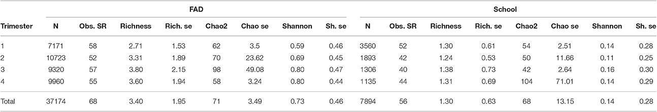
Table 1. Distribution of sets (N), Overall Observed Species richness (Obs. SR), Mean Species richness per set (Richness), Richness standard error (Rich. se), Chao2 non-parametric estimator, Chao2 standard error (Chao se), Mean Shannon diversity index per set (Shannon) and Shannon standard error (Sh. se) by trimesters in FAD and School sets.

FIGURE 1

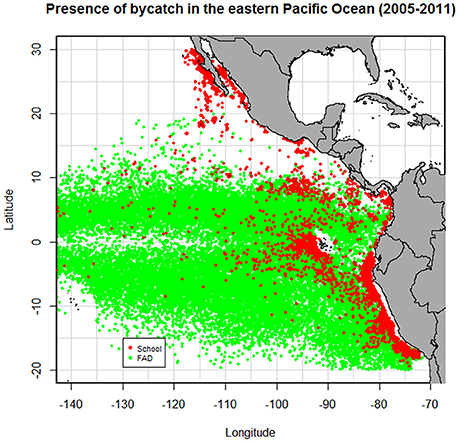
Figure 1. Distribution of sets with presence of bycatch in FAD and School fishing mode between 2005 and 2011.

Selection of Taxonomic Categories for Biodiversity Study

In the case of high level taxa records (genus, family, order and other levels), the distribution of species and their abundance was assigned based on the species composition for the same group (e.g., genus, family) in the same area (Lezama-Ochoa et al., 2015) for one particular year. As species level identification for the Families Belonidae, Diodotidae and Myliobatidae, and the Genus Sphyraena were not possible, they were considered as morphospecies -taxa that are distinguishable on the basis of the morphology (Oliver and Beattie, 1996)—and treated as species in species richness estimates (Lezama-Ochoa et al., 2015).

The list of species selected comprised a total of 72 species (6 billfish species, 20 sharks, 34 bony-fishes, 4 turtles and 8 species of rays).

Environmental Data

For each fishing set (date and position), which covered the period January 2005- December 2011, values of oceanographic variables were provided by CLS (Collecte Localisation Satellite, France, https://www.cls.fr) in the form of global geographic maps for each variable. Temperature at 20, 30, 50 and 75 m depth (SubT20, SubT30, SubT50, and SubT75; in °C); depth of the thermocline (Therm. Depth; in m); gradient of the thermocline (Therm. Grad; in °C); salinity at 20, 30, 50, and 75 m depth (Sal20, Sal30, Sal50, and Sal75; in PSU); and total surface current speed (WT; in kn) are outputs of MERCATOR general ocean circulation model (http://www.mercator-ocean.fr/en/), with a 25 Km spatial resolution and a frequency of 2/3 days. Sea Surface Temperature (SST; in °C) was derived from AVHRR and MODIS satellite data with 4 km resolution, acquired, respectively from NOAA CLASS (https://www.class.ncdc.noaa.gov/saa/products/welcome;jsessionid=64A6E9D799B84B49C1AEC15FB5A00900) and NASA OBPG (https://oceancolor.gsfc.nasa.gov). Chlorophyll concentration the same day of the fishing set and 18 days before (Chl and Chl-18 in mg m-3) with a 4 km resolution was derived from MODIS and MERIS satellite data, acquired, respectively from NASA OBPG and ESA. Sea Level Anomaly (SLA; in cm) and geostrophic current speed (WG; in kn) from altimetry were available with 25 km resolution. These altimetry maps were computed by CLS from different combinations of satellites ERS-2, Topex/Poseidon, Jason-1/2, ENVISAT, GFO, and CRYOSAT.

Methods

Alpha Diversity

Alpha diversity measures the species diversity of a particular community, defined by two components: the number of species present (species richness) and how even their numerical participation in the community is (evenness) (Magurran, 2004).

Alpha diversity's first component (species richness) was calculated as the total number of observed species and represented using species accumulation curves. This technique shows the cumulative number of species recorded as a function of the sampling effort (i.e., number of samples) or the rate at which new species are found within a community. As a result, a smooth curve is produced by repeating a process of randomly adding the samples to the accumulation curve and then plotting the mean of these permutations (normally as value of 100) (Coleman et al., 1982). All the possible species can be considered found when the asymptote of the curve is reached. In this work, a simulation (5 replicates) of species accumulation curves for both types of fishing selecting randomly the same number of sets (N = 1,000) were also carried out.

Some authors have demonstrated that a raw count of the number of species in an area is far from the best estimate of true species richness (Reese et al., 2014). Despite its wide appeal and apparent simplicity, accurate estimates of species richness can be remarkably difficult to achieve using only the observed number of species. For that reason, there are some extrapolation techniques, such as non-parametric estimators, which allow the total number of species to be estimated using solely information of the observed number of species (Magurran and McGill, 2011). The Chao2 non-parametric estimator (Chao, 1984) (which represents the asymptote of the species accumulation curve), which adjusts the observed species richness by the number of rare taxa defined on occurrence data, was also used to obtain the estimated total species richness vs. observed species richness.

The mean value of the Species richness index was also calculated to compare diversity of the bycatch assemblages between both fishing types and trimesters.

The relative abundance of a species in an assemblage is the main factor that determines its importance in a diversity measure (Magurran, 2004). Thus, the second component of Alpha diversity (evenness) is better to describe the variability in species abundances of an area. A community in which all species have approximately equal numbers of individuals would be considered as an extremely even community (Magurran, 2004).

One of the best known and most informative methods to study the relative abundance of species is the rank/abundance plot or dominance/diversity curve. The vertical axis provides information about the logarithm of abundance, while the horizontal axis provides information about the number of species.

The log-abundance curves represent the relative abundance of the species (number of individuals for each species) from the most abundant to the rarest one. In this work, log-rank abundance curves were constructed for each fishing mode (FAD vs. School) to obtain the abundance of each species.

The shape of the log-rank abundance for each fishing mode can be fitted to different species abundance models: Geometric, Log-series, Log-normal and Broken stick models (Magurran, 2004); which describe the structure of the community. Therefore, the slope of the rank abundance plot describes community structure and diversity. Steep slopes signify assemblages with a high dominance of few species, such as the one that might be found in a Geometric or Log-series distribution, while smaller slopes imply higher evenness, consistent with a Log-normal or a Broken stick model (Magurran, 2004). Whittaker (1965) indicated that low diversity communities are Geometric while medium diversity communities are Log-series and high diversity communities are Log-normal.

The data was fitted to the following species distribution models (using the “vegan” package and “radlattice” function in R software): Null model (or Broken Stick model), Pre-emption model (or Geometric model), Log-normal model, Zipf model and Zipf-Mandelbrot model. The functional form for each model is explained in Pielou (1975) and Wilson (1991). The best model fit, according to the lowest AIC value or Akaike's Information Criterion (Akaike, 1974), represents best the community structure (Kindt and Coe, 2005).

Other indices, such as the Shannon diversity index, which includes information not only about the number of species of the assemblage but also about the relative abundance (Magurran, 2004), were used.

The Shannon diversity index (Shannon and Weaver, 1949) is defined as,

$\begin{array}{l}\text{H}\prime =-\Sigma \text{pi ln }·\text{ pi}\end{array}$

where pi is the proportion of individuals of ith species found. Values range between 1.5 and 3.5; increasing diversity with the increase of the Shannon index. The mean value of the Shannon diversity index was calculated to compare diversity of the bycatch assemblages between both fishing types and by trimesters.

Geographical and Habitat Characteristics of Bycatch Species

Generalized Additive Models (GAMs) (Hastie and Tibshirani, 1990; Guisan et al., 2002) were constructed to identify the spatial and habitat characteristics of the bycatch species in relation with Species richness and Shannon diversity index between 2005 and 2011. Spatial (latitude and longitude), temporal (month), the type of association (FAD vs. School sets) and oceanographic variables were included in the analysis. The type of fishing was considered as covariate to determine if each bycatch species assemblage has different habitat characteristics. These models were chosen over generalized linear models as they are able of modeling continuous or categorical variables, replacing the linear function by a sum of smooth functions (Hastie and Tibshirani, 1990).

All environmental covariates were considered initially in the models, except those highly correlated between them (Pearson correlation r > 0.6) to avoid overfitting (Wood, 2006). Only one variable was included in the final model when high correlation was found between two variables.

To validate the model performance, a cross-validation was applied with a k-fold partitioning method (with k = 5) (Kohavi, 1995; Elith and Leathwick, 2009). Data was split into two different sets: one set used to fit the model (80% of data), called the training data, and the other set used to validate and obtain the predictions, called the testing data (20% of data).

The degrees of freedom of the smooth functions were determined for each explanatory variable as part of the model fitting process (Lopez et al., 2017). Each GAM was fitted using (i) thin plate regression splines to model nonlinear covariate effects, except for monthly variation, where a cyclic cubic regression spline was used (Wood, 2006) and (ii) a two-dimensional thin plate regression spline surface to account for spatial effects attributable to the location (latitude, longitude) of each fishing set (Lopez et al., 2017).

A GAM with a QuasiPoisson error distribution and logistic-link function was used to model the Species richness index. A GAM with a Gaussian error distribution with identity-link function was used to model the Shannon diversity index. The selection of the family and link function was determined by the distribution of the response variable for each index, respectively. In the case of Species richness index a slight over-dispersion of the response variable was observed; in contrast, for the Shannon index, the response variable showed a normal distribution.

The selection of the effective covariates to include in each GAM was performed applying backward stepwise procedure and selecting significant p-values for each geographical/oceanographic variable. The variables which explain the diversity patterns were considered as the variables included in the final model. After fitting the model, residuals were plotted and Spearman's rank correlation coefficient (rs) was calculated to evaluate the model accuracy. P-values lower than 0.05 and correlation coefficients higher than 0.1 provide good model accuracy (Lauria et al., 2011). Model bias was also evaluated using Wilcoxon's signed-rank test to compare observed vs. predicted values. This test compares the median observed vs. predicted diversity, to test biased in the predictions.

Predictions are considered bias (underestimated/overestimated) if test values are lower than 0.05 (Montero et al., 2016). Finally, the residuals were also plotted to obtain information about the fitting performance.

Spatial prediction maps of average, minimum, maximum and standard deviation of both diversity indices were calculated from the trained model and using only test data. Spatial prediction maps by fishing mode and trimesters were also produced using the corresponding testing data in each case.

All the analyses were carried out using “vegan” (Oksanen et al., 2013), “BiodiversityR” (Kindt and Kindt, 2015) and “mgcv” (Wood and Wood, 2007) packages of R-3.3.2 free software (R Core Team, 2016).

Results

Alpha Diversity

In general, both fishing modes showed different number of species (Table 1), with slightly higher number of species observed in FAD sets (68) in comparison with School sets (56). The simulation of species accumulation curves for both types of fishing showed similar number of total observed species between both fishing modes (Supplementary Material Figure 2). The Kruskall-Wallis statistical test showed not significant differences in the number of species between both fishing modes (Supplementary Material Figure 2) in the simulation.

The Chao2 estimator showed that a total of 71 and 68 species could be observed in FAD and School sets, respectively, if the sample size is large enough (ant in this case, represented by the asymptote in the species accumulation curves) (Table 1, Figure 2).

FIGURE 2

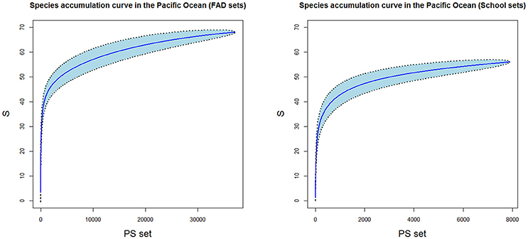
Figure 2. Species accumulation curves in FAD sets (A) and School sets (B). PS, purse seine set; S, species richness. Blue area corresponds to the standard deviation.

The most abundant species in FAD sets was the Coryphaena hippurus (2044000 individuals) and Caranx sexfasciatus (75299 individuals) in School sets. The 10 most abundant species formed 95.8% with respect the total species in FAD sets and 90.1% in School sets (Table 2). In both types of fishing, and with the exception of the silky shark (Carcharhinus falciformis), the most bycaught species were small bony-fishes.

TABLE 2

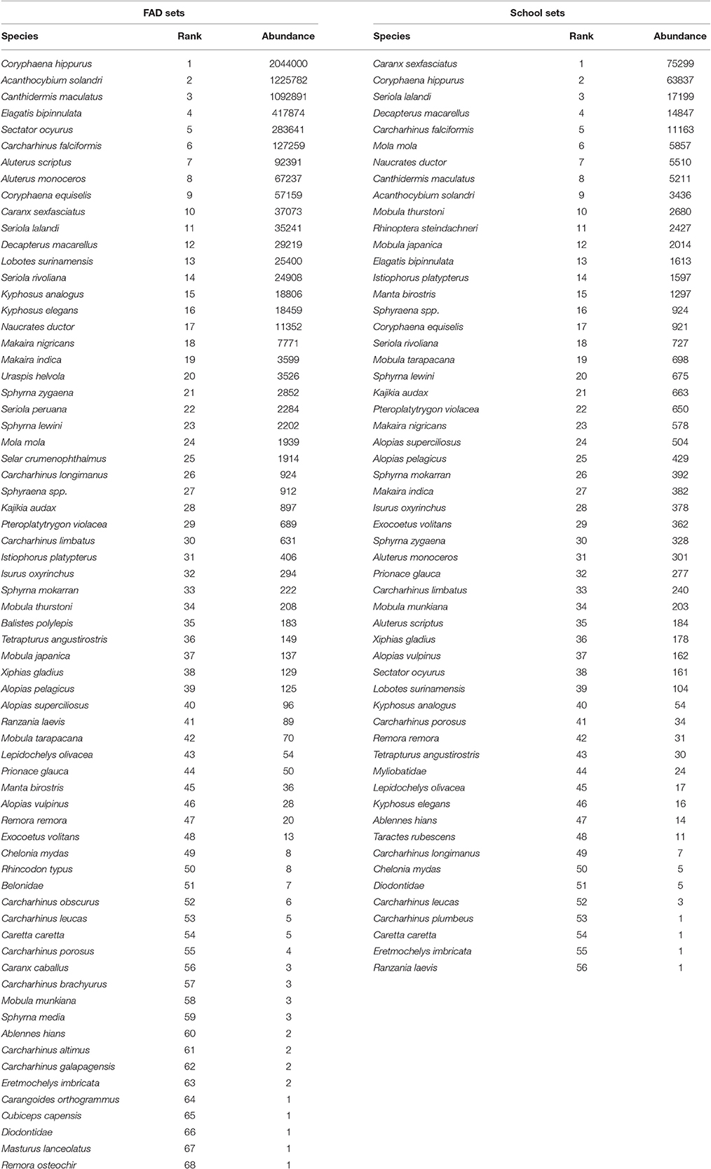
Table 2. Species abundance in FAD and School sets.

After fitting the different species abundance models to the rank abundance curves in both fishing modes, results showed that bycatch assemblages in FAD sets followed a Log-normal distribution, and the bycatch assemblages in School sets a Zipf-Mandelbrot distribution or Log-series distribution based on the lowest AIC values (Figure 3 and Supplementary Material Table 1). The shape of the curves lead us to suggest that bycatch species are more evenly distributed in FAD sets than in School sets.

FIGURE 3

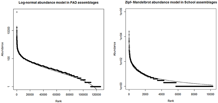
Figure 3. Models selected to fit log-rank abundance curves in FAD (A) and (B) School sets.

Finally, the mean Species richness and Shannon diversity index were calculated in both fishing modes and by trimesters and results are shown in Table 1. Bycatch assemblages have higher number of species (3.40) and diversity (0.73) in FAD sets than in School sets.

Mean richness and Shannon index, stratified by quarters in FAD and School sets showed high diversity in the third and fourth quarter (Table 1).

Geographical and Habitat Characteristics of Bycatch Species

The final model for species richness included as explanatory variables spatial variables (latitude-longitude interaction), temporal variables (month), type of fishing mode (type as factor) and environmental variables (sea surface temperature, chlorophyll and current speed).

$\begin{array}{l}\text{S}=\text{f}1(\text{Lon},\text{ Lat})+\text{ f}2(\text{SST})+\text{ f}3(\text{Chl})+\text{ f}4(\text{WT})\\ +\text{ f}5(\text{month})+\text{ type}\end{array}$

The estimated parameters for species richness and p-values are listed in Table 3 and Figure 4. The model explained 44% of the variance with a R2 of 0.38 with 39179 samples. The individual contribution of the variables is showed in Table 3; where the most significant explanatory variables for the species richness was the area (35%, lat*long) followed by set type (29%), chlorophyll (21%) and SST (17.5%). The correlations between the variables are showed in Supplementary Material Figure 3. The distribution of residuals is showed in Supplementary Material Figure 4. The Normal Q-Q plot showed a normal distribution; as well as the relationship between fitted and response values. The good distribution of residuals suggests a correct identification of areas of high diversity.

TABLE 3

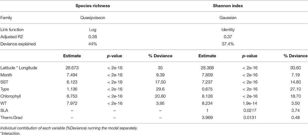
Table 3. Summary results for the optimal GAMs selected for Species richness index and Shannon diversity index.

FIGURE 4

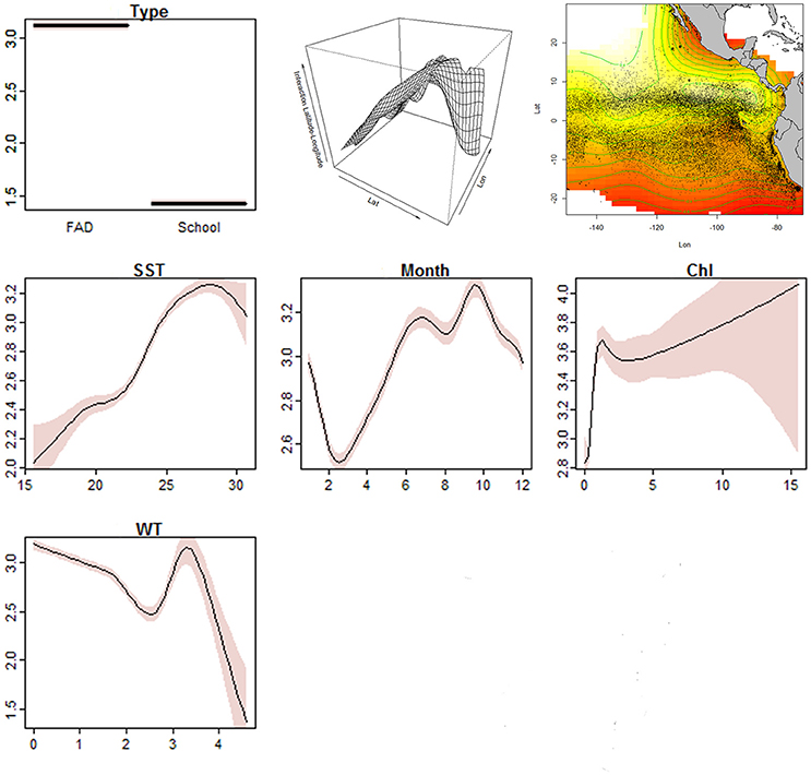
Figure 4. Smoothed fits of covariates modeling the Species richness index of diversity for: Type (FAD vs. School), Interaction (Lat*Lon), SST (sea surface temperature, in °C in x-axis), Month, Chl (chlorophyll, in mg m-3 in x-axis) and WT (total speed current, in knots in x-axis) variables. The y-axis represents the spline function. Dashed lines indicate approximate 95% confidence bounds.

Predictions from GAMs (mean, minimum, maximum and standard deviation) using testing data (20% of data) are shown in Figure 5. Predictions from GAMs by trimesters are shown in Figure 6.

FIGURE 5

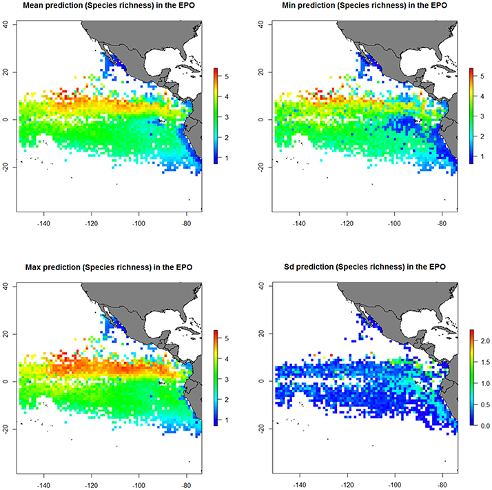
Figure 5. Predicted diversity (Species richness index) of the bycatch assemblages in FAD and School sets in the eastern Pacific Ocean (EPO) from the generalized additive model (GAM). Mean diversity (upper-left); Maximum diversity (bottom-left); Minimum diversity (upper-right); Standard deviation of diversity (bottom-right).

FIGURE 6

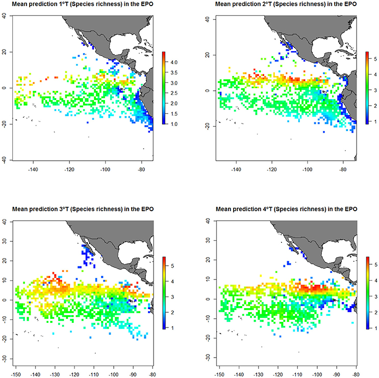
Figure 6. Predicted diversity (Species richness index) of the bycatch assemblages in FAD and School sets in the eastern Pacific Ocean (EPO) from the generalized additive model (GAM). Mean prediction for the first (1st T), second (2nd T), third (3rd T) and fourth trimester (4th T).

The results showed higher diversity observed in FAD sets than in School sets. Diversity was higher at north of the Equator (0–10°N) and at around 85–95°W and 120–140°W during May-November. Furthermore, highest richness values were found in areas with high sea surface temperatures (>25°C), high concentrations of chlorophyll (> 2 mg/m3), and velocities of the total current lower than 3 knots.

In order to relate Shannon diversity index with environmental variables in space and time, the final model includes Shannon diversity index as response variable, latitude and longitude as geographical variables (interaction), month as temporal variable, type of association as a factor and sea surface temperature, chlorophyll, gradient of the thermocline, sea level anomaly and velocity of the current as environmental variables.

$\begin{array}{l}\text{SH}=\text{f}1(\text{Lon},\text{ Lat})+\text{f}2(\text{SST})+\text{f}3(\text{Chl})+\text{f}4(\text{WT})\\ +\text{ f}5(\text{Therm}.\text{Grad})+\text{f}6(\text{SLA})+\text{f}7(\text{month})+\text{type}\end{array}$

Gaussian model for Shannon diversity index explained 37.4% of the variance with a R2 of 0.37 with 30081 samples (Table 3). Results showed similar diversity patterns as with species richness (Supplementary Material Figure 5) and therefore, only models with species richness were represented. Similar to species richness, the most significant explanatory variables (based on the individual contribution of each variable) for the Shannon diversity index was the area (31%, lat*long) followed by set type (27%), chlorophyll (19%), and SST (15%).

In general, predicted maps for both indices showed highest diversity around the Equatorial area and lowest diversity values were found along the Peru and California coast (Figure 5 and Supplementary Material Figure 5). Based on the predicted maps from GAMs, large diversity in FAD sets seems to be around the Equatorial area and in School sets around the Costa Rica Dome (Figure 7 and Supplementary Material Figure 5).

FIGURE 7

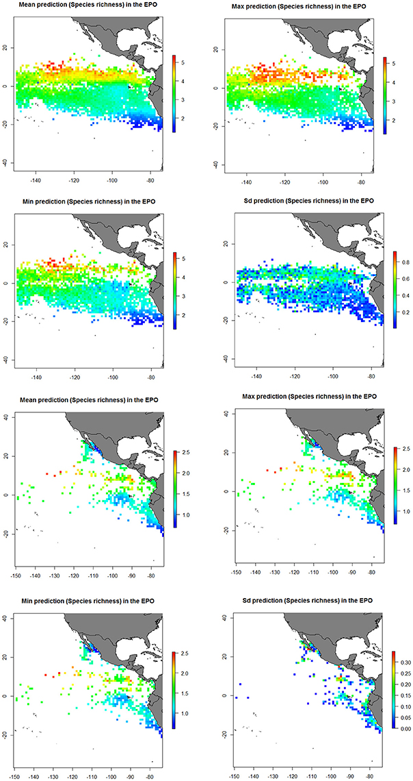
Figure 7. Predicted diversity (Species richness index) of the bycatch assemblages by type of set in the eastern Pacific Ocean (EPO) from the generalized additive model (GAM). Mean diversity; Maximum diversity; Minimum diversity and Standard deviation of diversity for FAD (upper four) and School sets (bottom four).

The evaluation of the models using Spearman's correlation showed a good model accuracy; with significant positive correlation between observed and predicted diversity for both indices (r = 0.62, p < 0.05 for Species richness index and r = 0.63, p < 0.05 for Shannon index). In contrast, Wilcoxon's signed-rank test showed significant p-values lower than 0.05 using the Species richness index, suggesting some bias in the model (Supplementary Material Table 2). The latter indicates that although the model is capable of describing the species richness of the bycatch species, the model overestimated and underestimated the observed values.

Discussion

This study examined the diversity of the bycatch assemblages with a variety of measures using data collected by observer programs from tropical tuna purse seine fishery in FAD and School sets. Results showed a variety of diversity patterns (based on the number of species and abundances) as a function of the time of year and fishing mode. Furthermore, they provided new information about the habitat characteristics of these species in the eastern Pacific Ocean. We suggest that both fishing modes represent different assemblages and therefore, the structure, diversity and environment characteristics of these bycatch assemblages and the areas where these species are found are also different.

Alpha Diversity

Species diversity of the bycatch assemblages could be a useful indicator, in conjunction with other ecosystem indicators, to monitor the ecosystem status and effect of the fishery in the ecosystem provided that a good sample size is available for a correct estimation of species diversity. Our results showed that the sample size used in this study with nearly 100% coverage rate was sufficient to find almost all species in FAD and School sets, as shown by the shape of the accumulation curves where the asymptote is reached. Although it is known that the number of species of the bycatch in FAD sets is higher than in School sets (Amandè et al., 2010; Torres-Irineo et al., 2014), our work suggests that the total number of bycatch species (and not the number of species per set) caught in the tropical tuna purse seiners is the same for both set types provided that sufficient sample size and the coverage rate is reached irrespective of the fishing mode.

As such, observer programs can provide the necessary information for diversity studies; but with limitations depending on the observer coverages. For example, lower sample size and coverage rate (around 10%) is available in other oceans and, therefore the results should be discussed taking into account the observer coverages. However, accumulation curves also showed that the asymptote was reached in some cases and, hence, species richness can be used as biodiversity measures in the Indian (Lezama-Ochoa et al., 2015) and Atlantic Ocean (Lezama-Ochoa et al., submitted). Differences in the number of the total observed species between fishing modes were more notable in the Indian and Atlantic Oceans, which could be explained by the lower coverage rate, especially for School sets, in these Oceans. Thus, sufficient observer coverage is needed to detect all the possible bycatch species in both types of fishing for biodiversity studies.

Our results suggest that Chao2 estimator, as used in the work of Torres-Irineo et al. (2014) and Lezama-Ochoa et al. (2015) is a good option for estimating the total species richness in both fishing modes. The Chao2 estimator showed that FAD and School sets could reach the asymptote with 71 and 68 species, respectively, which means that almost all species caught in the purse-seine fishery in the studied area were observed and the sample size was enough for obtaining bycatch diversity estimates. Chao2 non-parametric estimator is considered to be more accurate than parametric estimators or curve extrapolations (Gotelli and Colwell, 2011) to estimate total species richness (Chao, 1984). This is because it does not need any predetermined requirement as other models (Colwell and Coddington, 1994; Chao et al., 2005).

A evenly distributed species community is more diverse than a community with the same number of species but dominated by few species (Stirling and Wilsey, 2001). The shape of the log-abundance curves showed the same results than in Lezama-Ochoa et al. (2015) for both fishing modes in the Indian Ocean in relation with the species abundance models. In general, the Log-series distribution (Zipf model) model describes communities with higher number of rare species than the Log-normal model does. Bycatch assemblages in FAD sets are formed by permanent species (species which are aggregated under FADs for hours or days) in the same habitat and evenly distributed (Magurran, 2004), in large and natural areas (Log-normal model). On the contrary, bycatch species in School sets are formed by different and rare species that migrate in oceans for reproductive or feeding activities with migratory species, such as tunas (Zipf-Mandelbrot model) (Lezama-Ochoa et al., 2015). The structure of these bycatch assemblages let us to infer that both fishing modes represent different assemblages and therefore, with different characteristics.

Richness is commonly used as the sole measure of diversity, ignoring community evenness and species' relative abundances (Connolly et al., 2013). Log-abundance curves provide good information about the most common and rarest species; in our case, about bycatch species from the tropical tuna purse-seine fishery on the pelagic ecosystem. In this work, Coryphaena hippurus, was the bycatch species mostly caught in FAD sets and Caranx sexfasciatus in Free School sets. Species having life history strategies similar to the target species, such as teleost fishes (“r” strategist species), may not be affected to the same degree as those species with significantly different life history features, such as sharks (“k” strategist species) (Alverson, 1994). The most abundant species in this work are characterized by “r” strategies; with the exception of Carcharhinus falciformis, which is normally caught in FAD sets and is considered a more vulnerable species. Technological developments to mitigate incidental catch of vulnerable species, such as Carcharhinus falciformis are necessary to achieve effective fishery management and reduce their mortalities (Gilman, 2011). For example, in recent years, their survival rate has been increased by using new methods developed for mitigating the capture of sharks and other vulnerable species (Gilman, 2011; Poisson et al., 2014) in purse seiners.

Geographical and Habitat Characteristics of Bycatch Assemblages

Habitat distribution of pelagic communities normally match the distribution of water masses (Angel, 1993), but determination of the dominant factors influencing the distributions of these communities is difficult. In this work, GAMs contributed to relate diversity of the bycatch assemblages with the geographical and environmental conditions in the eastern Pacific Ocean.

Our results suggest that the geographical location and the type of set are the most important predictor variables to describe diversity for these species. Specifically, the highest predicted diversity of the bycatch species is on FAD sets compared to School sets. Differences found on diversity patterns between areas and fishing modes lead us to suggest that each bycatch species assemblage has different habitat characteristics. We observed a general diversity patterns on bycatch assemblages in both fishing modes. We found that bycatch assemblages are more diverse in equatorial areas in FAD sets and in warm coastal areas (Panama, Costa Rica and Nicaragua) in School sets (Figure 7). In contrast, the permanent coastal upwelling areas of California and Peru showed high productivity rates but low species diversity. These results, as described in Irigoien et al. (2004) and Sala and Knowlton (2006), showed that diversity in general in the open oceans, and particularly in the tropics, is lower at high disturbance levels and high productivity rates. More diverse communities are located in ecosystems with stable oceanographic conditions and less undisturbed (Cusson et al., 2014) (such as equatorial and seasonal coastal upwelling systems of this work), whereas permanent coastal upwelling areas support high disturbance levels with short trophic chains and, therefore, less diversity.

Diversity patterns of bycatch assemblages in both fishing modes in the eastern tropical Pacific match reasonably well with the principal characteristics of its oceanography, hydrography and circulation (Fiedler and Talley, 2006; Kessler, 2006; Lavín et al., 2006; Pennington et al., 2006). In the case of the environmental variables, the sea surface temperature and chlorophyll were the environment predictors that better explained diversity patterns (Table 3). Concretely, the higher values of diversity could be related to water masses associated with seasonal coastal and equatorial upwelling processes. Thus, diversity patterns from the models indicated that bycatch assemblages in FAD sets could be associated with the equatorial tongue (10°N–5°S/120°–140°W) (from August to October) which is developed when the southeast trade winds are strongest during southern Winter (Wyrtki, 1981), with the North Equatorial Countercurrent, and with two physical features particularly significant in the Tropical Surface Water (TSW): the Equatorial Front (Fiedler and Talley, 2006) and the countercurrent thermocline ridge (along 10°N) (Ballance et al., 2006; Hoegh-Guldberg and Bruno, 2010).

All these sites are characterized by warm waters (>25°C) with low-salinity and intermediate productivity concentrations, strong currents and with great biological significance, where marine predators and prey may aggregate during September-October.

In the case of the bycatch assemblages in School sets, results from the model (low thermocline gradients and high chlorophyll concentrations) lead us to suggest that highest species diversity could be associated with coastal upwelling regions around Costa Rica and Panama in the equatorial area (Costa Rica Dome and Gulf of Panama) (10–20°S/80–100°W). Located within the warm pool and with low thermocline depth, these warm, productive and low-salinity waters are affected by the wind jets in winter (Pennington et al., 2006). Thus, winter northwesterly strong winds, most intense from November to March (Pennington et al., 2006; Change, 2007), induce upwelling of colder and nutrient-rich waters to the surface, giving place to cool and very productive, but stable surface waters.

Importance of Ecosystem Indicators for Fisheries Management

Biodiversity indices provide information on trends in species diversity regarded as important by society and have potential to inform on progress toward established management objectives (Hutchings and Baum, 2005). In that sense, biodiversity is a concept with multiple meanings which can be measured in different ways (Buckland et al., 2005). In this work, we considered the number of species and the relative abundance of them as good measures to describe the biodiversity of the bycatch assemblages. Both types of fishing should be considered to estimate species diversity indices and patterns, as the integration of data from both fishing modes provides more complete information (spatially and temporally) than separately. Nonetheless, as more species are attracted to FADs due to species aggregative behavior, more specific works are necessary to understand the complete effect of the FAD fishery on the biodiversity of the bycatch at local (specific areas) and global (Oceans) scale.

Despite the fact that trends in biodiversity can vary enormously between areas or habitats, observer programs should be designed to monitor this spatial variation (Buckland et al., 2005). These differences in biodiversity between areas could be explained by the fact that some species are restricted to some areas but, in some cases, also as a consequence of the different fishing effort, time of year or many other possible factors, such as environmental events (e.g., ENSO cycle). The major limitation of this study is the use of fisheries-dependent data, which is focused on catching tuna, not bycatch species. Thus, diversity patters could be partially biased by the nature of the data and fishery behavior (Montero et al., 2016). Although in the Atlantic and Indian Oceans the observer coverage is low (around 10% of coverage rate) (Lewison et al., 2004), which can compromise the analysis and results (Lennert-Cody, 2001), the high coverage of the eastern Pacific Ocean increase the representativeness of the estimates. IATTC observer programs in the eastern Pacific Ocean provide important information for evaluating spatial-temporal variability of fish assemblages and impacts of commercial fisheries on the most vulnerable species (Montero et al., 2016). In that sense, the IATTC purse-seine database covers a large area and period of years compared with the other Oceans, so the information about the species involved is of high quality and quantity; even considering the limitations mentioned above (Montero et al., 2016). Anyway, the inclusion of fisheries independent data would considerable contributes to improve the conclusions of this study.

Conclusion

This work has improved our understanding of diversity and habitat characteristics of the bycatch assemblages in the eastern Pacific Ocean. Indicators based on the number of species in a community and the relative abundance of them (richness and evenness) were calculated. Moreover, diversity and the environmental characteristics of the bycatch species in the eastern Pacific Ocean were explained based on both fishing modes (i.e., FAD and School sets). The prediction of diversity was good, with 40% of the variation explained by the models. Modeling the biodiversity of bycatch using data from observer programs provide new and useful information for future management plans. This study contributed to the understanding and integration of different components of the ecosystem in order to progress in the implementation an Ecosystem Approach Fishery Management.

Author Contributions

NL, HM, MH, MR, JR, NV, AC, and IS designed research; NL, HM, and MH performed research; NL analyzed data; and NL, HM, MH, and AC wrote the paper.

Funding

This study was part of the PhD thesis (Lezama-Ochoa, 2016) conducted by the first author (NLO) at AZTI-Tecnalia marine institute and funded by Iñaki Goenaga (FCT grant). The authors declare that the publication of this work is in line with the author's university policy. This is contribution 824 from AZTI-Tecnalia Marine Research Division.

Conflict of Interest Statement

The authors declare that the research was conducted in the absence of any commercial or financial relationships that could be construed as a potential conflict of interest.

Acknowledgments

The observer data analyzed in this study was collected by IATTC observer programs and the oceanographic data has been provided by the CLS (https://www.cls.fr). Thanks to Robert Olson for his comments and suggestions.

Supplementary Material

The Supplementary Material for this article can be found online at: https://www.frontiersin.org/article/10.3389/fmars.2017.00265/full#supplementary-material

References

Akaike, H. (1974). A new look at the statistical model identification. Autom. Contr. IEEE Trans. 19, 716–723. doi: 10.1109/TAC.1974.1100705

CrossRef Full Text | Google Scholar

Alverson, D. L. (1994). A Global Assessment of Fisheries Bycatch and Discards. FAO Fisheries Technical Paper. Rome: Food & Agriculture Org.

Google Scholar

Amandè, M. J., Ariz, J., Chassot, E., De Molina, A. D., Gaertner, D., Murua, H., et al. (2010). Bycatch of the European purse seine tuna fishery in the Atlantic Ocean for the 2003–2007 period. Aquat. Living Resour. 23, 353–362. doi: 10.1051/alr/2011003

CrossRef Full Text | Google Scholar

Angel, M. V. (1993). Biodiversity of the pelagic ocean. Conserv. Biol. 7, 760–772. doi: 10.1046/j.1523-1739.1993.740760.x

CrossRef Full Text | Google Scholar

Arrizabalaga, H., Murua, H., and Majkowski, J. (2012). Global status of tuna stocks: summary sheets. Rev. Invest. Mar. 19, 645–676.

Google Scholar

Ballance, L. T., Pitman, R. L., and Fiedler, P. C. (2006). Oceanographic influences on seabirds and cetaceans of the eastern tropical Pacific: a review. Prog. Oceanogr. 69, 360–390. doi: 10.1016/j.pocean.2006.03.013

CrossRef Full Text | Google Scholar

Buckland, S., Magurran, A., Green, R., and Fewster, R. (2005). Monitoring change in biodiversity through composite indices. Philos. Trans. R. Soc. B Biol. Sci. 360, 243–254. doi: 10.1098/rstb.2004.1589

PubMed Abstract | CrossRef Full Text | Google Scholar

Change, I. P. O. C. (2007). Climate Change 2007: The Physical Science Basis. Paris: Agenda 6, 333.

Google Scholar

Chao, A. (1984). Nonparametric estimation of the number of classes in a population. Scand. J. Stat. 11, 265–270.

Google Scholar

Chao, A., Chazdon, R. L., Colwell, R. K., and Shen, T. J. (2005). A new statistical approach for assessing similarity of species composition with incidence and abundance data. Ecol. Lett. 8, 148–159. doi: 10.1111/j.1461-0248.2004.00707.x

CrossRef Full Text | Google Scholar

Coleman, B. D., Mares, M. A., Willig, M. R., and Hsieh, Y.-H. (1982). Randomness, area, and species richness. Ecology 63, 1121–1133. doi: 10.2307/1937249

CrossRef Full Text | Google Scholar

Colwell, R. K., and Coddington, J. A. (1994). Estimating terrestrial biodiversity through extrapolation. Philos. Trans. R. Soc. Lond. B Biol. Sci. 345, 101–118. doi: 10.1098/rstb.1994.0091

PubMed Abstract | CrossRef Full Text | Google Scholar

Connolly, J., Bell, T., Bolger, T., Brophy, C., Carnus, T., Finn, J. A., et al. (2013). An improved model to predict the effects of changing biodiversity levels on ecosystem function. J. Ecol. 101, 344–355. doi: 10.1111/1365-2745.12052

CrossRef Full Text | Google Scholar

Cullis-Suzuki, S., and Pauly, D. (2010). Failing the high seas: a global evaluation of regional fisheries management organizations. Mar. Policy 34, 1036–1042. doi: 10.1016/j.marpol.2010.03.002

CrossRef Full Text | Google Scholar

Cusson, M., Crowe, T. P., Araújo, R., Arenas, F., Aspden, R., Bulleri, F., et al. (2014). Relationships between biodiversity and the stability of marine ecosystems: comparisons at a European scale using meta-analysis. J. Sea Res. 98, 5–14. doi: 10.1016/j.seares.2014.08.004

CrossRef Full Text | Google Scholar

Dayton, P. K., Thrush, S. F., Agardy, M. T., and Hofman, R. J. (1995). Environmental effects of marine fishing. Aqua. Conserv. 5, 205–232. doi: 10.1002/aqc.3270050305

CrossRef Full Text | Google Scholar

Duffy, L. M., Olson, R. J., Lennert-Cody, C. E., Galván-Magaña, F., Bocanegra-Castillo, N., and Kuhnert, P. M. (2015). Foraging ecology of silky sharks, Carcharhinus falciformis, captured by the tuna purse-seine fishery in the eastern Pacific Ocean. Mar. Biol. 162, 571–593. doi: 10.1007/s00227-014-2606-4

CrossRef Full Text | Google Scholar

Elith, J., and Leathwick, J. R. (2009). Species distribution models: ecological explanation and prediction across space and time. Annu. Rev. Ecol. Evol. Syst. 40, 677–697. doi: 10.1146/annurev.ecolsys.110308.120159

CrossRef Full Text | Google Scholar

Fiedler, P. C. (1992). Seasonal Climatologies and Variability of Eastern Tropical Pacific Surface Waters. NOAA/National Marine Fisheries Service, NOAA Technical Report NMFS, 109.

Fiedler, P. C., and Talley, L. D. (2006). Hydrography of the eastern tropical Pacific: a review. Prog. Oceanogr. 69, 143–180. doi: 10.1016/j.pocean.2006.03.008

CrossRef Full Text | Google Scholar

Garcia, S. M. (2003). The Ecosystem Approach to Fisheries: Issues, Terminology, Principles, Institutional Foundations, Implementation and Outlook. FAO Fisheries Technical Paper. Rome: Food & Agriculture Org.

Google Scholar

Gilman, E. L. (2011). Bycatch governance and best practice mitigation technology in global tuna fisheries. Mar. Policy 35, 590–609. doi: 10.1016/j.marpol.2011.01.021

CrossRef Full Text | Google Scholar

Gotelli, N. J., and Colwell, R. K. (2011). Estimating species richness. Biol. Divers. 12, 39–54.

Google Scholar

Greenstreet, S. P., and Rogers, S. I. (2006). Indicators of the health of the North Sea fish community: identifying reference levels for an ecosystem approach to management. ICES J. Mar. Sci. 63, 573–593. doi: 10.1016/j.icesjms.2005.12.009

CrossRef Full Text | Google Scholar

Guisan, A., Edwards, T. C. Jr., and Hastie, T. (2002). Generalized linear and generalized additive models in studies of species distributions: setting the scene. Ecol. Modell. 157, 89–100. doi: 10.1016/S0304-3800(02)00204-1

CrossRef Full Text | Google Scholar

Hall, M. A., Alverson, D. L., and Metuzals, K. I. (2000). By-catch: problems and solutions. Mar. Pollut. Bull. 41, 204–219. doi: 10.1016/S0025-326X(00)00111-9

CrossRef Full Text | Google Scholar

Hall, M., and Roman, M. (2013). Bycatch and Non-Tuna Catch in the Tropical Tuna Purse Seine Fisheries of the World. FAO Fisheries and Aquaculture Technical Paper 568.

Hastie, T. J., and Tibshirani, R. J. (1990). Generalized Additive Models. CRC Press.

PubMed Abstract | Google Scholar

Hoegh-Guldberg, O., and Bruno, J. F. (2010). The impact of climate change on the world's marine ecosystems. Science 328, 1523–1528. doi: 10.1126/science.1189930

PubMed Abstract | CrossRef Full Text | Google Scholar

Hutchings, J. A., and Baum, J. K. (2005). Measuring marine fish biodiversity: temporal changes in abundance, life history and demography. Philos. Trans. R. Soc. B Biol. Sci. 360, 315–338. doi: 10.1098/rstb.2004.1586

PubMed Abstract | CrossRef Full Text | Google Scholar

IATTC (2010). Inter-American Tropical Tuna Commission (IATTC). 2010. Fishery Status Report n 7. La Jolla, CA: IATTC.

IATTC (2015). Inter-American Tropical Tuna Commission (IATTC). 2015. Annual Report. La Jolla, CA: IATTC.

Irigoien, X., Huisman, J., and Harris, R. P. (2004). Global biodiversity patterns of marine phytoplankton and zooplankton. Nature 429, 863–867. doi: 10.1038/nature02593

PubMed Abstract | CrossRef Full Text | Google Scholar

Kessler, W. S. (2006). The circulation of the eastern tropical Pacific: a review. Prog. Oceanogr. 69, 181–217. doi: 10.1016/j.pocean.2006.03.009

CrossRef Full Text | Google Scholar

Kindt, R., and Coe, R. (2005). Tree Diversity Analysis: A Manual and Software for Common Statistical Methods for Ecological and Biodiversity Studies. Nairobi: World Agroforestry Centre.

Google Scholar

Kindt, R., and Kindt, M. R. (2015). Package BiodiversityR.

Kohavi, R. (1995). “A study of cross-validation and bootstrap for accuracy estimation and model selection,” in Proceedings of the 14th International Joint Conference of Artificial Intelligence (IJCAI), Vol. 2, (Montreal, QC: Morgan Kaufmann), 1137–1145.

Lauria, V., Vaz, S., Martin, C. S., Mackinson, S., and Carpentier, A. (2011). What influences European plaice (Pleuronectes platessa) distribution in the eastern English Channel? Using habitat modelling and GIS to predict habitat utilization. ICES J. Mar. Sci. 68, 1500–1510. doi: 10.1093/icesjms/fsr081

CrossRef Full Text | Google Scholar

Lavín, M. F., Fiedler, P. C., Amador, J. A., Ballance, L. T., Färber-Lorda, J., and Mestas-Nuñez, A. M. (2006). A review of eastern tropical Pacific oceanography: summary. Prog. Oceanogr. 69, 391–398. doi: 10.1016/j.pocean.2006.03.005

CrossRef Full Text | Google Scholar

Lennert-Cody, C. (2001). Effects of sample size on bycatch estimation using systematic sampling and spatial post-stratification: summary of preliminary results. IOTC Proc. 4, 48–53.

Google Scholar

Lewison, R. L., Crowder, L. B., Read, A. J., and Freeman, S. A. (2004). Understanding impacts of fisheries bycatch on marine megafauna. Trends Ecol. Evol. 19, 598–604. doi: 10.1016/j.tree.2004.09.004

CrossRef Full Text | Google Scholar

Lezama-Ochoa, N. (2016). Biodiversity and Habitat Preferences of the By-Catch Communities from the Tropical Tuna Purse-Seine Fishery in the Pelagic Ecosystem: The Case of the Indian, Pacific and Atlantic Oceans. PhD Thesis. Department of Zoology and Animal Cell Biology, University of the Basque Country, 282.

Lezama-Ochoa, N., Murua, H., Chust, G., Ruiz, J., Chavance, P., de Molina, A. D., et al. (2015). Biodiversity in the by-catch communities of the pelagic ecosystem in the Western Indian Ocean. Biodivers. Conserv. 24, 2647–2671. doi: 10.1007/s10531-015-0951-3

CrossRef Full Text | Google Scholar

Link, J. (2010). Ecosystem-Based Fisheries Management: Confronting Tradeoffs. New York, NY: Cambridge University Press.

Google Scholar

Lopez, J., Moreno, G., Lennert-Cody, C., Maunder, M., Sancristobal, I., Caballero, A., et al. (2017). Environmental preferences of tuna and non-tuna species associated with drifting fish aggregating devices (DFADs) in the Atlantic Ocean, ascertained through fishers' echo-sounder buoys. Deep Sea Res. II Top. Stud. Oceanogr. 140, 127–138. doi: 10.1016/j.dsr2.2017.02.007

CrossRef Full Text | Google Scholar

Magurran, A. E. (2004). Measuring Biological Diversity. Cornwall: Blackwell.

Google Scholar

Magurran, A. E., and McGill, B. J. (2011). Biological Diversity: Frontiers In Measurement And Assessment. New York, NY: Oxford University Press.

Google Scholar

Montero, J. T., Martinez-Rincon, R. O., Heppell, S. S., Hall, M., and Ewal, M. (2016). Characterizing environmental and spatial variables associated with the incidental catch of olive ridley (Lepidochelys olivacea) in the Eastern Tropical Pacific purse-seine fishery. Fish. Oceanogr. 25, 1–14. doi: 10.1111/fog.12130

CrossRef Full Text | Google Scholar

Oksanen, J., Blanchet, F. G., Kindt, R., Legendre, P., Minchin, P. R., O'Hara, R., et al. (2013). Package ‘vegan.’ R Packag Version.

Oliver, I., and Beattie, A. J. (1996). Designing a cost-effective invertebrate survey: a test of methods for rapid assessment of biodiversity. Ecol. Appl. 6, 594–607. doi: 10.2307/2269394

CrossRef Full Text | Google Scholar

Olson, R. J., Duffy, L. M., Kuhnert, P. M., Galván-Magaña, F., Bocanegra-Castillo, N., and Alatorre-Ramírez, V. (2014). Decadal diet shift in yellowfin tuna Thunnus albacares suggests broad-scale food web changes in the eastern tropical Pacific Ocean. Mar. Ecol. Prog. Ser. 497, 157–178. doi: 10.3354/meps10609

CrossRef Full Text | Google Scholar

Olson, R. J., Popp, B. N., Graham, B. S., López-Ibarra, G. A., Galván-Magaña, F., Lennert-Cody, C. E., et al. (2010). Food-web inferences of stable isotope spatial patterns in copepods and yellowfin tuna in the pelagic eastern Pacific Ocean. Prog. Oceanogr. 86, 124–138. doi: 10.1016/j.pocean.2010.04.026

CrossRef Full Text | Google Scholar

Pennington, J. T., Mahoney, K. L., Kuwahara, V. S., Kolber, D. D., Calienes, R., and Chavez, F. P. (2006). Primary production in the eastern tropical Pacific: a review. Prog. Oceanogr. 69, 285–317. doi: 10.1016/j.pocean.2006.03.012

CrossRef Full Text | Google Scholar

Pielou, E. (1975). Ecology Diversity. New York, NY: Wiley, J. and Sons.

Pikitch, E. K., Santora, C., Babcock, A., Bakun, E. A., Bonfil, R., Conover, D. O., et al. (2004). Ecosystem-based fishery management. Science 305, 346–347. doi: 10.1126/science.1098222

PubMed Abstract | CrossRef Full Text | Google Scholar

Poisson, F., Séret, B., Vernet, A.-L., Goujon, M., and Dagorn, L. (2014). Collaborative research: Development of a manual on elasmobranch handling and release best practices in tropical tuna purse-seine fisheries. Mar. Policy 44, 312–320. doi: 10.1016/j.marpol.2013.09.025

CrossRef Full Text | Google Scholar

R Core Team (2016). R: A Language and Environment for Statistical Computing. Vienna: R Foundation for Statistical Computing.

Reese, G. C., Wilson, K. R., and Flather, C. H. (2014). Performance of species richness estimators across assemblage types and survey parameters. Global Ecol. Biogeogr. 23, 585–594. doi: 10.1111/geb.12144

CrossRef Full Text | Google Scholar

Sala, E., and Knowlton, N. (2006). Global marine biodiversity trends. Annu. Rev. Environ. Resour. 31, 93–122. doi: 10.1146/annurev.energy.31.020105.100235

CrossRef Full Text | Google Scholar

Scott, M. D., Chivers, S. J., Olson, R. J., Fiedler, P. C., and Holland, K. (2012). Pelagic predator associations: tuna and dolphins in the eastern tropical Pacific Ocean. Mar. Ecol. Prog. Ser. 458, 283–302. doi: 10.3354/meps09740

CrossRef Full Text | Google Scholar

Shannon, C. E., and Weaver, W. (1949). Themathematical Theory of Communication. Urbana: University of Illinois Press.

Smeets, E., Weterings, R., and voor Toegepast-Natuurwetenschappelijk, N. C. O. (1999). Environmental Indicators: Typology and Overview. Copenhagen: European Environment Agency Copenhagen.

Stirling, G., and Wilsey, B. (2001). Empirical relationships between species richness, evenness, and proportional diversity. Am. Nat. 158, 286–299. doi: 10.1086/321317

PubMed Abstract | CrossRef Full Text | Google Scholar

Torres-Irineo, E., Amandè, M. J., Gaertner, D., de Molina, A. D., Murua, H., Chavance, P., et al. (2014). Bycatch species composition over time by tuna purse-seine fishery in the eastern tropical Atlantic Ocean. Biodivers. Conserv. 23, 1157–1173. doi: 10.1007/s10531-014-0655-0

CrossRef Full Text | Google Scholar

Whittaker, R. H. (1965). Dominance and Diversity in Land Plant Communities Numerical relations of species express the importance of competition in community function and evolution. Science 147, 250–260. doi: 10.1126/science.147.3655.250

PubMed Abstract | CrossRef Full Text | Google Scholar

Wilson, J. B. (1991). Methods for fitting dominance/diversity curves. J. Vegetation Sci. 2, 35–46. doi: 10.2307/3235896

CrossRef Full Text | Google Scholar

Wood, S. (2006). Generalized Additive Models: An Introduction with R. Boca Ratón, FL: CRC Press.

Google Scholar

Wood, S., and Wood, M. S. (2007). The Mgcv Package. Available online at: www.r-project.org.

Worm, B., Barbier, E. B., Beaumont, N., Duffy, J. E., Folke, C., Halpern, B. S., et al. (2006). Impacts of biodiversity loss on ocean ecosystem services. Science 314, 787–790. doi: 10.1126/science.1132294

PubMed Abstract | CrossRef Full Text | Google Scholar

Worm, B., Sandow, M., Oschlies, A., Lotze, H. K., and Myers, R. A. (2005). Global patterns of predator diversity in the open oceans. Science 309, 1365–1369. doi: 10.1126/science.1113399

PubMed Abstract | CrossRef Full Text | Google Scholar

Wyrtki, K. (1981). An estimate of equatorial upwelling in the Pacific. J. Phys. Oceanogr. 11, 1205–1214.

Google Scholar

Zhu, J., Dai, X., and Chen, Y. (2011). Species composition and diversity of pelagic fishes based on a longline fishery catch in the North Pacific Ocean. Chin. J. Oceanol. Limnol. 29, 261–269. doi: 10.1007/s00343-011-0122-7

CrossRef Full Text | Google Scholar