Evaluation, Gap Analysis, and Potential Expansion of the Finnish Marine Protected Area Network

Introduction

Marine ecosystems are facing unprecedented loss of biodiversity due to habitat destruction, a changing marine environment and increasing resource extraction (Worm et al., 2006; Halpern et al., 2008, 2015). A key aspect in safeguarding marine biodiversity is the design of ecologically effective networks of Marine Protected Areas (MPAs). Especially no-take reserves have been shown to support high biodiversity and food web complexity (Halpern and Warner, 2002; Lester et al., 2009; Halpern, 2014). Increased emphasis is required on an ecologically efficient MPA design and sustainable management, to ensure that MPAs achieve global conservation objectives (Edgar et al., 2014).

International agreements require nations to establish ecologically coherent MPA networks to support and maintain marine processes and functions (CBD, 2004; Directive, 2008). In 2010, the Convention on Biological Diversity (CBD) agreed on the Aichi biodiversity target 11, stating that by 2020 at least 10% of coastal and marine areas should be conserved and effectively managed. The areas under protection need to fulfill four criteria: adequacy, representativity, replication and connectivity, in order to be ecologically efficient (CBD, 2010; HELCOM, 2010). In addition, in 2014, the World Parks Congress urged that at least 30% of each marine habitat should be under strict protection thus increasing the previous recommendation of at least 20% protected (Wenzel et al., 2016). This ambitious recommendation known as the Promise of Sydney highlights progress in marine protection in recent years.

In Europe, the cornerstone of conservation has been the Habitats Directive (CD 92/43/EEC) (EC, 1992). It aims to maintain an adequate conservation status for habitats and species, listed in Annexes I and II. Over 200 habitats are protected by the Directive, identified as either biogeographically important or being in danger of disappearing. It is the responsibility of the Member States to ensure that adequate conservation status is achieved by designating areas for protection, with habitats listed in Annex I of the Directive as the key selection criteria for Natura 2000 sites (Evans, 2012).

The challenge is to establish MPAs in areas where they provide the highest conservation benefits for the marine environment. Designation of MPAs has in many areas mostly relied on ad hoc decisions and not necessarily on knowledge on marine habitats and species (Agardy et al., 2011). Consequently, it has been concluded that the majority of MPAs fail to meet their management objectives (Jameson et al., 2002; Edgar et al., 2014). Furthermore, as MPAs often focus on conserving habitats or individual species, but not on the functionality of the marine ecosystem, the true ecological efficiency of the networks has mostly remained obscure. Studies about the effectiveness and performance of MPAs have, for example, evaluated effects on coastal fish (Sundblad et al., 2011; Olsen et al., 2013; Gill et al., 2017), broad-scale habitats (Foster et al., 2017), or shellfish (Fariñas-Franco et al., 2018). Especially if MPA designation allows significant resource use, as is the case for most MPAs globally, one may be skeptical about the effectiveness of MPA status (Sala et al., 2018). Unfortunately, data needed for the assessment of the functioning of MPA networks is often missing.

The brackish and semi-enclosed Baltic Sea is ecologically unique, as it possesses steep horizontal and vertical environmental gradients in salinity and temperature, and hosts a mixture of marine and freshwater species. Due to the low salinity (0–7 PSU) in the northern Baltic Sea, diversity of benthic species, especially benthic animals and marine algae, is low. In contrast, the low salinity enables a variety of vascular plants to grow along the shallow water areas of the Baltic Sea (Bonsdorff, 2006; Ojaveer et al., 2010; HELCOM, 2012; Zettler et al., 2014). Long scientific tradition, experience in cross-border environmental management, and a long-term struggle against multiple pressures, such as chemical pollution, eutrophication, non-indigenous species and habitat destruction, makes the Baltic Sea an ideal test case for other coastal and marine systems world-wide tackling with similar problems (Reusch et al., 2018). The Baltic Sea was also one of the first regional seas in the world to reach the Aichi target 11 (EEA, 2015). Qualified MPAs in the Baltic Sea consist of: HELCOM MPAs – aiming to protect Baltic biodiversity, EU marine Natura 2000 sites – protecting habitats and species, Ramsar sites – protecting important wetlands, and national parks and nature reserves.

Finland has an important role in the conservation efforts of the Baltic Sea, not only because of the long coastline (48,000 km) and large number of islands (∼100,000) (Viitasalo et al., 2017), but also because Finland has since 1930 systematically developed its protected area network. Presently 10% of the Finnish sea areas (including EEZ) are under protection. The Finnish MPAs consist of Natura 2000 sites (8.5%), HELCOM MPAs (7.7%), Ramsar sites (2.2%), National Parks (1.9%), private MPAs (1.8%) and Nature Reserves (0.7%) and (MPAtlas, 2018) (one MPA can belong to more than one MPA class.) While they cover extensive sea areas, MPAs in Finland and elsewhere in the Baltic Sea have often been established to protect habitats, bird areas, seals, or terrestrial environment on islands and skerries, without prior knowledge of underwater species or nature values in general. It is also notable that while many human activities are restricted within MPAs, no-take zones for fishing are rare amongst the Finnish MPA network. This leaves an important part of the ecosystem without any protection.

A proper evaluation of the ecological coherence of MPAs requires extensive data and suitable analytical tools. A major project for the improvement of ecological knowledge of marine nature started in 2004, known as the Finnish Inventory Programme for the Underwater Marine Environment VELMU. The project has produced the most extensive dataset on marine biodiversity to date in the Baltic Sea, with ∼140,000 standardized sampling sites. The data collected, along with data on environmental parameters and human activities, is viewable at the VELMU Map Service paikkatieto.ymparisto.fi/VELMU_mapservice/. Here, we take advantage of this new data by building new models that describe distributions of species and utilize other existing data on habitats as well as fish reproduction areas. In addition, we develop estimates for marine pressures that contribute to the decline and loss of important marine habitats.

Methodologically, our work relies on the Zonation method and software designed for ecologically based land use planning (Moilanen et al., 2005, 2011a; Lehtomaki and Moilanen, 2013). Zonation produces a hierarchical prioritization across the landscape, balanced across many factors such as species, habitats, ecosystem services and connectivity, and accounting for costs and/or threats if sufficient data exists. Most applications of Zonation have been terrestrial, but there have been some marine applications as well. For example, Leathwick et al. (2008) used Zonation to evaluate a proposed MPA network in New Zealand, with the conclusion that the proposal was of fractional quality compared to what could have been achieved using Zonation, and with zero cost to fishermen. Analytically, it makes no difference whether data grids represent terrestrial or marine biodiversity.

The new extensive data and novel models combined with spatial prioritization allow the first comprehensive assessment in the Baltic Sea of how well the present MPA network protects marine features of highest ecological value. Going further, our analysis identifies new MPA candidates that would improve the conservation coverage achieved by the MPA network efficiently. With the analysis we are also able to assess if the habitats protected by the EU Habitats Directive Annex I can be used as a proxy for safeguarding biodiversity, which allows an evaluation of the fundamental conservation principles implemented in the EU. We also assess the state and quality of marine habitats and identify areas where additional habitat protection is needed. This is the first time that any country in the Baltic Sea has data available at a spatial scale and resolution that enables identifying where the biologically most valuable marine areas are located. The analysis implemented here can serve as a template and a recipe for similar analyses in the Baltic Sea and also in other sea areas elsewhere in the world.

Materials and Methods

Study Area

Our analysis area consists of Finnish territorial waters and exclusive economic zone (EEZ), covering 21% (81,500 km²) of the Baltic Sea. Steep environmental gradients of salinity, turbidity, exposure and geomorphology characterize the Finnish marine areas, forming harsh marine habitats and conditions, where adaptation and specialization is necessary for survival. To the north, Bothnian Bay is shallow and low-saline, with exposed shores and monotonic geomorphology. The Quark, located in the middle of the Gulf of Bothnia, acts as a dividing biogeographical line between the north and south, beyond which survival of many marine species becomes impossible. Continuing south from the Quark, the Archipelago Sea with its 52,500 islands constitutes one of the most complex archipelago systems in the world (Viitasalo et al., 2017). In contrast to the north, marine areas in the south are more impacted by various physical and human-induced pressures that weaken water quality. For instance, the Gulf of Finland, the easternmost stretch of the Baltic Sea, is heavily burdened by eutrophication and frequent hypoxia.

Data Acquisition and Pre-processing

Species Data

The Finnish Inventory Programme for the Underwater Marine Environment (VELMU) has gathered information on species, communities and habitats during 2004–2016 from ∼140.000 locations. Video observations form the bulk of the data together with a reputable ∼28,000 diving sites (Figure 1) and an additional 2,889 benthic fauna samples.

FIGURE 1

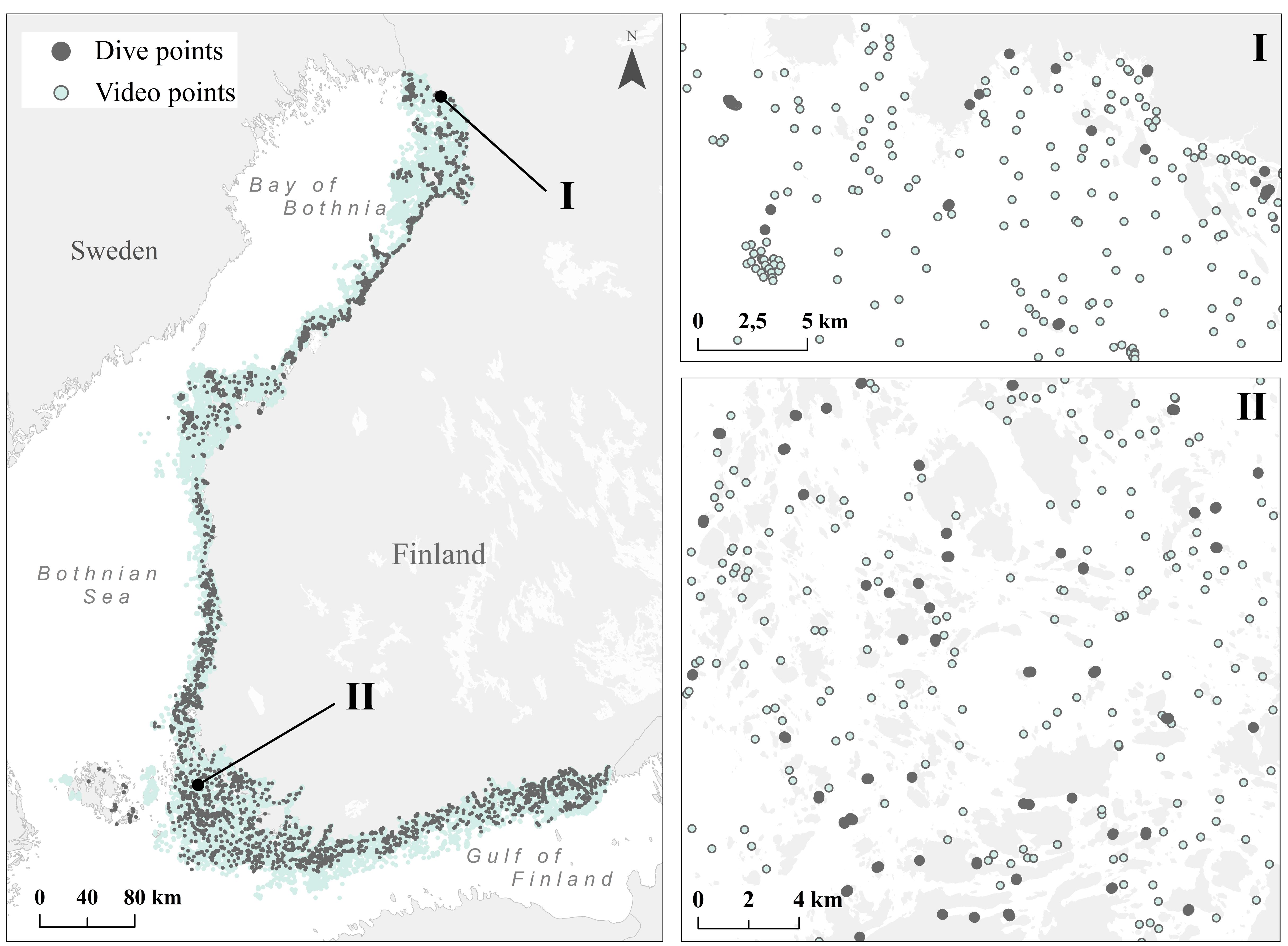
FIGURE 1. Dive (gray) and video (blue) points collected during the VELMU project 2004–2016 with zoomed-in example areas from the Bothnian Bay (I) and the Archipelago Sea (II).

The mean density of observation sites for videos is ∼4/km², and for dive sites ∼3/km² above 30 m depth, if considering areas where VELMU inventories are targeted. Most of the data represent rather shallow waters, where macrophytes dominate. In addition to the VELMU project, data from areas suitable for bottom fauna exist from other projects and national monitoring programs (see the section “Modeling of Species Distributions”). Observations are distributed in the marine space mostly through random stratified sampling; representing different environmental conditions, ranging from saline, exposed marine areas to enclosed, low-saline shallow bays. During the study years, additional targeted sampling has been conducted based on certain specific criteria, such as endangered species, certain marine environments and specific vulnerable habitats. Overall, these data provide an exceptionally good basis for ecosystem-based marine spatial planning and for analyses on marine biodiversity.

Habitat Data

The EU Habitats Directive aims to protect Annex I Habitats (from here on referred as marine habitats). Of the listed habitat types, 69 occur in Finland, of which eight are associated with marine environments: (1) Baltic esker islands (1610), (2) Boreal Baltic islets (1620), (3) Boreal Baltic narrow inlets (1650), (4) Coastal lagoons (1150), (5) Estuaries (1130), (6) Large shallow inlets and bays (1160), (7) Sand banks (1110), and (8) Reefs (1170). Here, we utilized the existing models for (1), (2), (7), and (8) (Rinne et al., 2014; Kaskela and Rinne, 2018) and GIS datasets for other marine habitats, based on expert knowledge reported for the EU in 2013 (EEA, 2013). Existing data on fish reproduction areas (Kallasvuo et al., 2016) were also used in the conservation prioritization part (see the section “Spatial Prioritization”), and are considered here as a proxy for biodiversity of juvenile fish.

Marine Environment Data

As Finland hosts extensive environmental gradients (see the section “Study Area”), we developed layers describing the varying nature of marine environments; seabed topography, hydrographical parameters, light conditions and eutrophication (Table 1).

TABLE 1

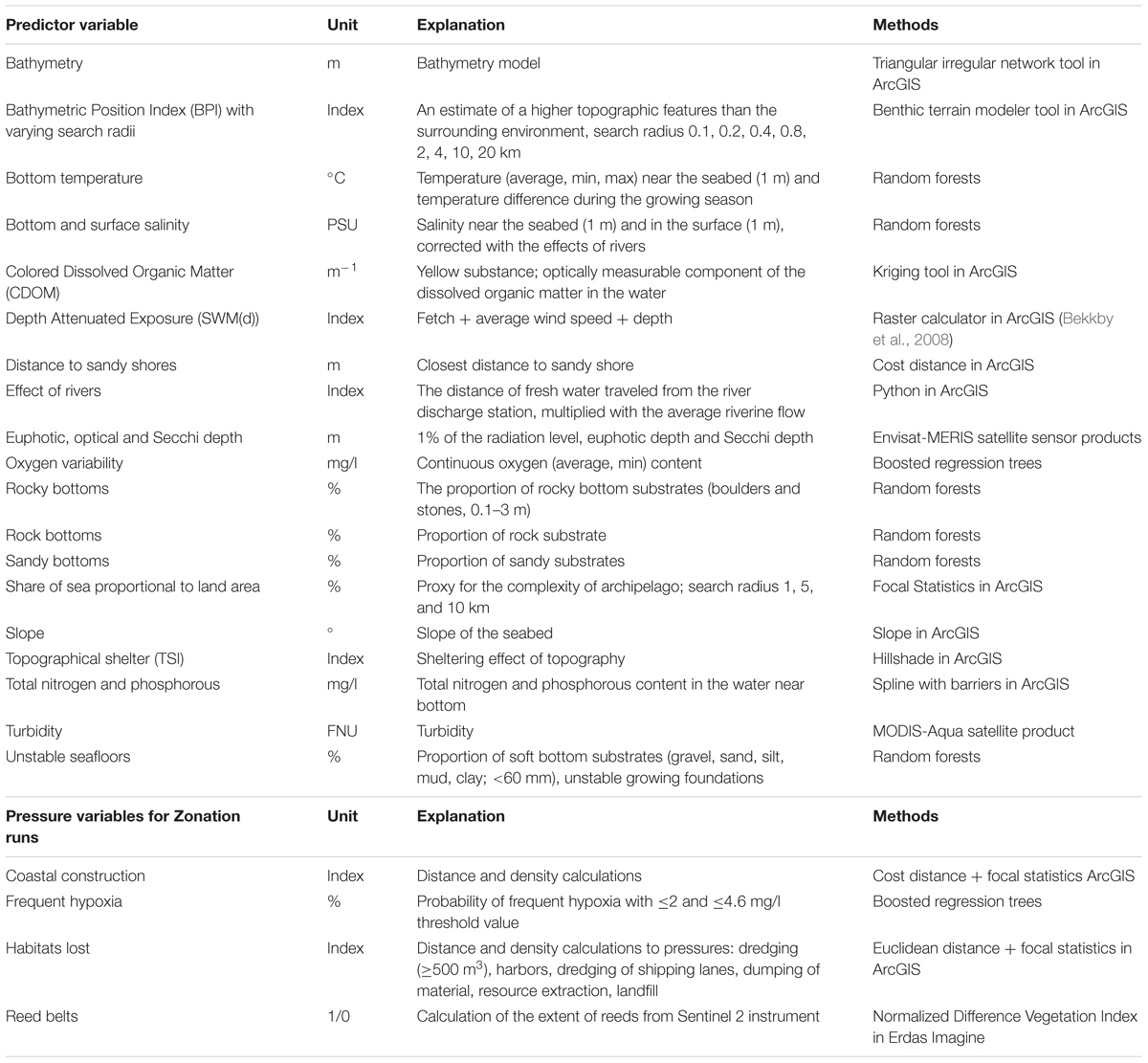
TABLE 1. Environmental predictor variables developed and compiled for the statistical distribution modeling of the species, communities and IUCN Red List of ecosystems, and marine pressures utilized in the prioritization.

Marine Pressures

Habitat loss is the greatest threat to biodiversity (Hanski, 2011). In the marine realm, habitats are lost due to direct/indirect human activities, e.g., coastal construction, modification of the seabed or natural causes, e.g., hypoxia. Modification of the seabed leads to habitat loss, degradation and/or to the disturbance of habitats (Sundblad and Bergström, 2014). Here, we consider activities that directly modify the seabed: dredging of shipping lanes (Finnish Transport Agency), harbors (from CORINE database), landfill, dumping of material (from VESTY database), and resource extraction (gravel, sand) (from databases of Parks and Wildlife Finland). Other harmful activities considered here are coastal construction (Finnish Transport Agency) (due to constant disturbance, e.g., marinas), reed belts (occupation of habitat at the expense of other species), eutrophication, and hypoxia (see Table 1). For habitats lost and coastal construction, we followed the approach by Sundblad and Bergström (2014) with slight modifications. We calculated the Euclidean distance to each activity, with a 25 m buffer for coastal construction, and 50 m buffer for activities leading to habitat loss. Using ArcGIS Focal Statistics, we estimated the density of activities at the 20 m grid resolution used in analysis. In Zonation analysis, different weights were given for marine pressures depending on the level of impact of each pressure (see the section “Feature Weights and Connectivity”).

Modeling of Species Distributions

Species distribution models (SDMs) are commonly used to inform a variety of ecological questions regarding, e.g., conservation planning, changing climate and biogeographical patterns (Leathwick et al., 2008; Elith et al., 2010). SDMs in essence describe the ecological niche of a species in geographical–environmental space. There are several estimation techniques for developing SDMs and the most extensively used ones are correlative approaches, in which species occurrences are linked to environmental data, and the resulting ecological niche is extrapolated to new (non-inventoried) geographical regions (Elith and Leathwick, 2009). SDMs are under-utilized in the marine realm if compared to terrestrial environments (Robinson et al., 2011), although modeling in the marine environment follows similar principles (cf. (Wilson et al., 2011; Elsäßer et al., 2013; Gormley et al., 2013; Howell et al., 2016; Jonsson et al., 2018).

Boosted regression trees (BRT), an ensemble method from statistical and machine learning traditions (De’ath and Fabricius, 2000; Hastie et al., 2001; Schapire, 2003), was utilized here to predict the probability of occurrence distribution and abundance patterns for alga, bryophytes, invertebrates, and vascular plants. BRT combines multiple best models instead of just one, and optimizes the output with the ability to model interactions and by identifying the most relevant predictor variables, thus outperforming the prediction performance of other methods. As BRT is a common approach for developing SDMs, we do not repeat a description of the technique here, as it has been thoroughly described elsewhere (cf. Elith et al., 2008). SDMs were developed for (i) most common and widespread species (e.g., clasping-leaf pondweed Potamogeton perfoliatus), (ii) key and habitat-forming species (e.g., bladderwrack Fucus spp. and blue mussel Mytilus trossulus x edulis), (iii) threatened species (e.g., Baltic water-plantain Alisma wahlenbergii), (iv) rare and sparsely occurring species (e.g., eelgrass Zostera marina), (vi) non-indigenous species (e.g., zebra mussel Dreissena polymorpha) and (vii) habitat types based on IUCN Red List of Ecosystems (from here on referred as IUCN Red List of Ecosystems, e.g., dominating benthic habitats characterized by red algae).

Random subsets (bag fraction) of data (50–80%) were used in the BRT modeling. The contribution of each tree to the next model (learning rate) was controlled by the cross-validated change in model deviance. Tuning of model parameters in general was dependent on sample size and the prevalence of the response variable, affecting the choice of learning rate. Higher tree complexities required slower learning rates (e.g., rare species), and vice versa.

Predictor selection is an automated process in BRT, as the algorithm ignores irrelevant variables in the model building. Predictor selection was performed only for the small datasets (i.e., rarely occurring species), where excess predictors increase the model variance. For modeling rare and threatened species with few occurrences, we applied the methodology of Ensemble of Small Models (ESM) for BRT (Breiner et al., 2015, 2018), and built models for the species in question with only a subset of two predictors, and then averaging the model output by weighted performance of each model (model fit correlations were kept above 0.7). Performances of SDMs were estimated with deviance explained, and the cross validated Area Under the Receiver Operating Characteristic curve (cvAUC), a measure of detection accuracy of true and false positives and negatives (Jiménez-Valverde and Lobo, 2007). AUC values above 0.9 indicate excellent, 0.7–0.9 good, and below 0.7 poor predictions.

Species records above a certain presence threshold were used in the BRT model iteration, depending on the model in question. In general, a threshold value of 0.1% was used for species distribution and abundance models and 10% for IUCN Red List of Ecosystems (Supplementary Table S1). Habitat is considered dominant, if at least one of the species, or combined coverages of all species, exceeds 50%. In addition, points evaluated for each substrate type were combined into a total coverage, and sampling points on the terrestrial side (e.g., due to land uplift) were removed. After this data pruning the total amount of data for modeling consisted of ∼137,000 samples. As more accurate information is gained by diving than from video methods, dive data was used as the primary source for modeling with 75–90% for model training and 10–25% for validation. The secondary source, video data, was used only for species clearly identifiable from videos with additional subsets (25%) from targeted inventories. As for invertebrates, additional data collated from national data repositories was used in two ways: (1) modeling of invertebrate distributions and abundances, and (2) as known macrophytes absence samples from deep, soft bottoms. Dive and video data are limited to rather shallow depths (typically 20–30 m), leading to a situation where there are not enough samples from deep areas (below 50 m). To avoid artifacts in the models, a randomized absence dataset for areas deeper than 50 m was used during the modeling process. These points were used only as absences in macrophytes models, based on the knowledge that macrophytes do not live at such depths in the Baltic Sea due to habitat constraints and lack of light.

Models were fitted in R 3.1.2. (R Core Team, 2017) with the gbm and dismo libraries, where additional, relevant functions were available for ecological data post-processing (Elith et al., 2008). Table 1 summarizes the explanatory variables used (excluding marine pressures) in this modeling, which was implemented at a 20 m resolution across the Finnish EEZ, leading to an effective grid size of 205 million elements (grid cells) per layer. As the topography and geomorphology of Finnish sea areas is very complex, such a high-resolution analysis is necessary to gain understanding about distributions of species and ecosystems. We point out that most of the variables used here include information that has never been available previously. The distribution models developed here were used in the subsequent Zonation analysis as is, retaining full spatial resolution and full information about probabilities of occurrence and abundances. Mixing of data types is automatically supported by Zonation (next section) and no thresholding of input data layers is needed.

Spatial Prioritization

General Approach Using Zonation

Zonation is an approach and software for ecologically based spatial prioritization, for the purposes of conservation planning, zoning, spatial impact avoidance, and other similar applications (Moilanen et al., 2005; Lehtomaki and Moilanen, 2013; Di Minin et al., 2014). It is capable of high-resolution, large extent, ecologically informed planning, with up to tens of thousands of layers of biodiversity distribution information used in analysis (Kremen et al., 2008; Pouzols et al., 2014). In addition to distribution information for biodiversity features, Zonation can account for factors such as connectivity, ecosystem services, costs, threats, etc., of course conditional on the availability of appropriate input data layers (Kareksela et al., 2013, 2018; Di Minin et al., 2017). As Zonation has been extensively described elsewhere, only a general description of Zonation is repeated here. See e.g., Lehtomaki and Moilanen (2013) and Di Minin et al. (2014) for an introduction to Zonation and interpretation of its outputs.

Zonation starts from the full landscape (seascape) and produces a spatial priority map by iterative ranking and removal of those grid cells that can be lost with smallest aggregate loss for biodiversity. This implies that areas to receive lowest ranks include hypoxic bottoms and areas where strong pressures have degraded water quality and habitats. Areas receiving highest ranks are the ones that host many species, ecosystems and habitats, including rare and highly weighted ones. A very important Zonation method is a form of analysis specifically developed for answering questions about PA network expansion (often called hierarchic analysis), in which the priority ranking is developed in two (or more) steps constrained by land use, land ownership or some other similar factor. In the present case, the hierarchic ranking was constrained by the present MPA network [see e.g., Mikkonen and Moilanen (2013) and Pouzols et al. (2014) for structurally identical analyses]. Doing a two-level ranking allows identification of those areas outside the MPA network, which increases conservation coverage of species and habitats in a balanced and area-efficient manner.

It should be noted that Zonation is not based on direct summing of layers. During iteration, it tracks what is remaining for each feature, and if a feature suffers loss (as is inevitable), the importance of its remaining occurrences goes up relative to features that do not suffer a loss at that particular ranking iteration (Moilanen et al., 2005). (As an associated technical detail, Zonation operates on normalized distributions, the fraction of distribution each grid cell holds for each feature (Moilanen et al., 2005, 2011a).) This process maintains a balance between all input features throughout the prioritization run. Factors such as ecological connectivity, feature weights and costs can (optionally) influence the balance between features through the prioritization process.

An overview of the present prioritization analyses is shown in Figure 2. Distribution models described in the previous section were used to form the marine nature values and to evaluate the performance of the present MPA network.

FIGURE 2

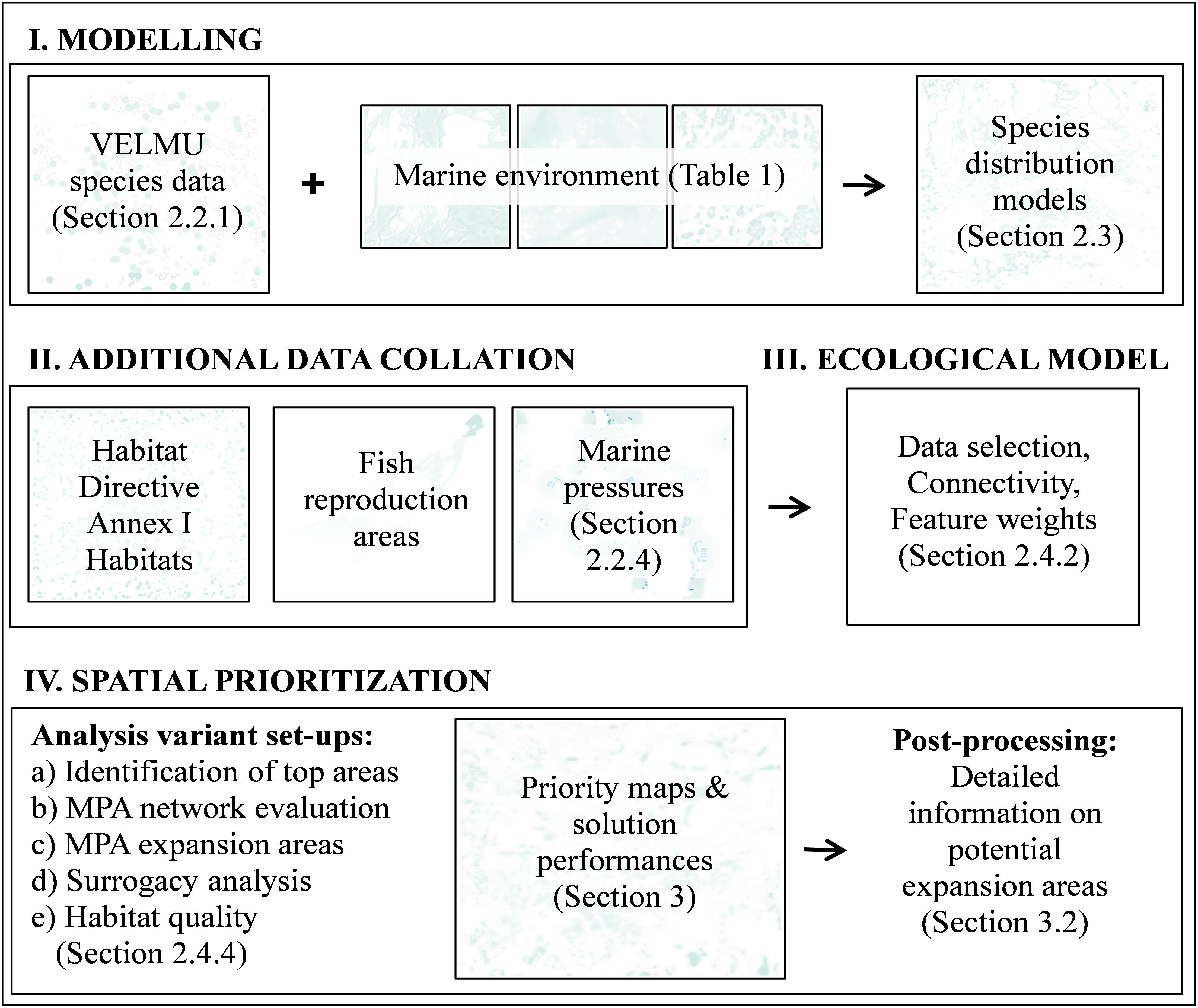
FIGURE 2. Schematic of work flow for spatial prioritization. Spatial prioritization starts with the data acquisition process. In this case data on species, environments, habitats, and human activities was collated, and pre-processed, for spatial prioritization by statistical modeling and extrapolation over the seascape at a high resolution of 20 m.

Feature Weights and Connectivity

An integral part of Zonation analyses is the setting of weights. As a starting point, all features are equally weighted. Then again, there are numerous reasons why the weight of a feature might be modified, including Red List status, phylogenetic uniqueness, functional position, economic importance, or relative uncertainty of information (Lehtomaki and Moilanen, 2013). Often, a hierarchic way of assigning weights is adopted. Relative weights are first assigned to high-level data blocks, such as species, habitats and ecosystem services. Then, inside these blocks additional modifying criteria, such as those listed above, are used to modify weights given to individual features. Also here, we applied hierarchic setting of weights. Based on data quantity and importance, we first assigned relative weights of 3:1:1 to species, marine habitats, and the IUCN Red List of Ecosystems. Here, species become somewhat emphasized, the rationale being the comparatively large number of high-quality distribution models available. Within species, habitats and ecosystems, certain factors were utilized to modify relative weights of features (Table 2). Note that even when species as a group receive a higher relative weight than environments, an individual habitat layer becomes weighted higher than an average species layer, as the feature count is higher for species than for habitats. Having individual habitats weighted higher than individual species is logically consistent, as habitats act as surrogates for many species, including those for which no data and distribution models exist.

TABLE 2

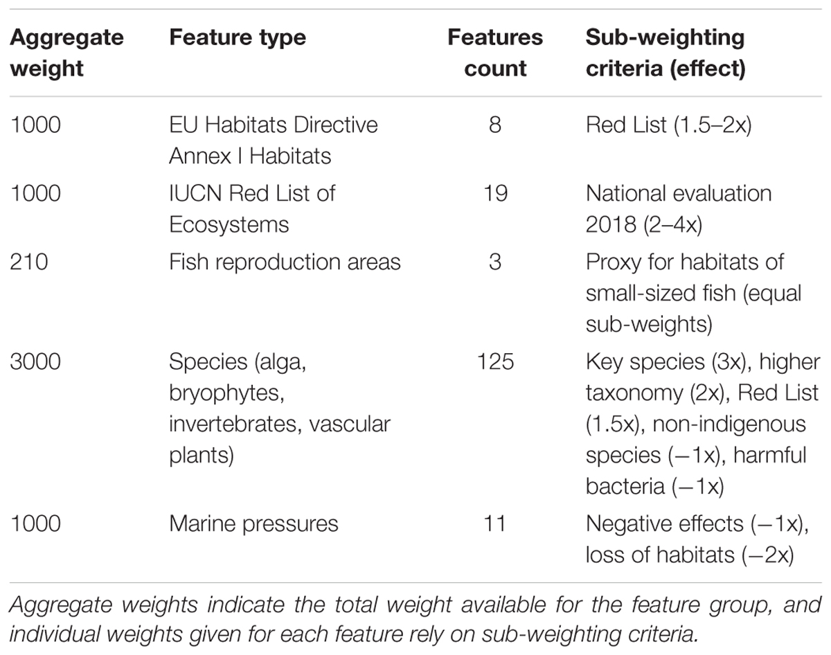
TABLE 2. Criteria used to moderate feature weights in the Zonation analyses.

Additional sub-weighting criteria were used inside relative weights for major data blocks (Table 2). Habitats and ecosystems received individually elevated weights based on Red List status, whereas species were weighted higher if considered a key species, a species (indicator) representing a broader species group (higher taxonomy, spp.), or if the species was listed as threatened (Red List) or vulnerable (HELCOM, 2013a). Fish reproduction areas represent important fish habitats thereby receiving elevated weights. Marine pressures were weighted higher (negative) based on the expected magnitude of the negative effect on marine conservation value. Species, habitats and ecosystems are given positive weights, as seen as valuable in the Zonation analysis, whereas pressures are given negative weights because environments are in better condition and conservation is easier away from the pressures. As a final detail relevant to weights, the Zonation algorithm itself already fully accounts for the distribution size of each feature; for instance, rare species (with very small distribution ranges) are automatically kept in the iteration process nearly until the end.

Connectivity is an integral component of spatial analyses, and becomes relevant at a high resolution (as in this study), because individual small areas are linked to their neighborhood. Connectivity was induced into solutions using two very basic methods, with the primary objective of accomplishing such aggregation that would facilitate the logistics of decision making. These techniques are called matrix connectivity and edge removal. Matrix connectivity identifies and enables connectivity of similar habitats and on the other hand of habitats close to each other (Lehtomäki et al., 2009). For instance in the marine realm, reefs and islets would benefit from connectivity, as they both host similar species, compared to areas with no potential habitats, such as deep, dark, soft bottoms. Here matrix connectivity between different marine habitat types was accounted for using a spatial scale of 200 m (mean decay distance in a declining-by-distance spatial kernel). The other connectivity technique used here, edge removal, constrains Zonation so that grid cells can only be ranked and removed at the edges of remaining areas, which to a small extent promotes maintenance of structural continuity of priority areas. No species-specific connectivity responses were used even though Zonation has several available. See Lehtomaki and Moilanen (2013) and Di Minin et al. (2014) for references and summary of connectivity options in Zonation.

Zonation Analysis Settings

Zonation requires decision about certain analysis settings that influence the prioritization. Zonation includes several ways of aggregating conservation value across many biodiversity features. From alternatives available, we used one called the additive benefit function (ABF), which tracks feature performance along individual species-area curves, aiming at minimization of aggregate expected extinction risk (Moilanen, 2007; Moilanen et al., 2011a). This is a good choice especially when biodiversity data available are seen as a surrogate for all biodiversity, which would also include species, habitats, and other factors not directly represented by data.

The dataset used has a large spatial dimension, 205 million effective grid cells at the spatial resolution of 20 m. In order to accelerate computational times, we aggregated (summed) data into 40 m grid cells. Planning units of this size are sufficient for marine spatial planning and conservation management purposes. An acceleration factor (called warp factor) of 5000 was used, implying that each algorithm iteration the 5000 grid cells leading to lowest loss in conservation value were ranked and removed from the remaining seascape. Despite the acceleration, the resolution of the x-axis in the performance curves (see Results) is higher than 0.01%, which is sufficient for all practical applications.

Analysis Variants and Post-processing

A standard technique of contrasting analysis variants computed under different assumptions was used also here to gain useful information. (i) Comparison between unconstrained analysis and one that accounts for the present MPA network - allows evaluation of present MPA network quality, see e.g., Mikkonen and Moilanen (2013). (ii) Contrast between solutions with and without additional structural connectivity - allows verification that additional connectivity can be achieved with acceptably low ecological price in terms of local coverage of features. (iii) Cross-evaluation of analyses based on species versus environments allows evaluation of how well species act as surrogates for marine habitats and vice versa. In addition to comparative analyses, we evaluated (iv) the state and quality of marine habitats and (v) the quality of existing MPAs. This information was obtained from standard Zonation post-processing analyses and additional GIS work.

Zonation post-processing analyses allow access to feature-level information about individual areas or area networks. Here, we used an analysis that allows getting information for pre-specified areas (groups of grid cell) that are identified to Zonation by inputting an additional mask file (landscape mask; LSM analysis) in which each area of interest is identified by a unique integer code (details in Moilanen and Kujala, 2014). Here, MPAs were categorized into: (1) HELCOM MPAs, (2) National parks, (3) Natura 2000 sites, (4) Nature reserves, (5) Private MPAs, and (6) Ramsar sites. Utilizing information from LSM post-processing, each individual MPA site was evaluated based on mean rank and feature density. The mean rank is the average of pixel-specific rank values from the priority rank map. Feature density of area i (FD_i) is the so-called distribution sum of the area divided by the distribution sum expected if all features were evenly distributed across the seascape. It can be calculated:

$$F{D}_{\mathrm{i}}=\frac{D{S}_{\mathrm{i}}\ast C}{A_{\mathrm{i}}\ast TDS},\mathrm{\hspace{0.17em}}\mathrm{in}\mathrm{\hspace{0.17em}}\mathrm{which}$$

DS_i = distribution sum of focal area i,

C = number of effective cells in the whole landscape,

A_i = number of grid cells in the focal area, and

TDS = total distribution sum of all features across the entire study area.

The same operation was carried out for habitats in order to evaluate the quality of each habitat type and to identify good-quality habitat patches outside the existing MPA network.

The last part of the work was to identify potential MPA network expansion areas, which was primarily based on information gained from the hierarchical prioritization that accounts for the present MPA network. Expansion candidate areas were identified taking the highest ranked 3% of areas outside the present MPA network, which were filtered according to size (>1 km²), leading to a net 1% expansion of protected sea area. The limit of 1% was chosen for illustrative purposes – we expect that decision makers might well appreciate how much can be achieved starting from a modest 1% expansion consisting of comparatively large areas. Establishment of new MPAs carries an administrative burden, and very small MPAs would likely not be favored. Additionally, conservation value hotspots were identified. This was done by combining the priority rank map and the weighted range-size rarity map (i.e., weighted range-size corrected richness map), another standard output from Zonation analyses. The first of these describes a relative ranking that is balanced across features and the latter is a weighted sum that emphasizes locations having many features in them. The combination of the two has increased emphasis on species richness and ecosystem function compared to the priority rank map. Conservation value hotspots were identified from a 500 m moving window calculation applied on the product map.

Results

Modeling

Species distribution models were produced for 19 IUCN Red List of Ecosystems and for over 100 taxa representing algae, invertebrates and vascular plants, summarized in Figure 3 and details in (Supplementary Table S1). Overall, models performed well, as cross-validated AUC values were above 0.7 (standard errors ± 0.09), and median percent deviance, a goodness-of-fit measure, varied from 71 to 87% on withheld test data. These SDMs have comprehensive coverage of marine biodiversity and thus conservation values.

FIGURE 3

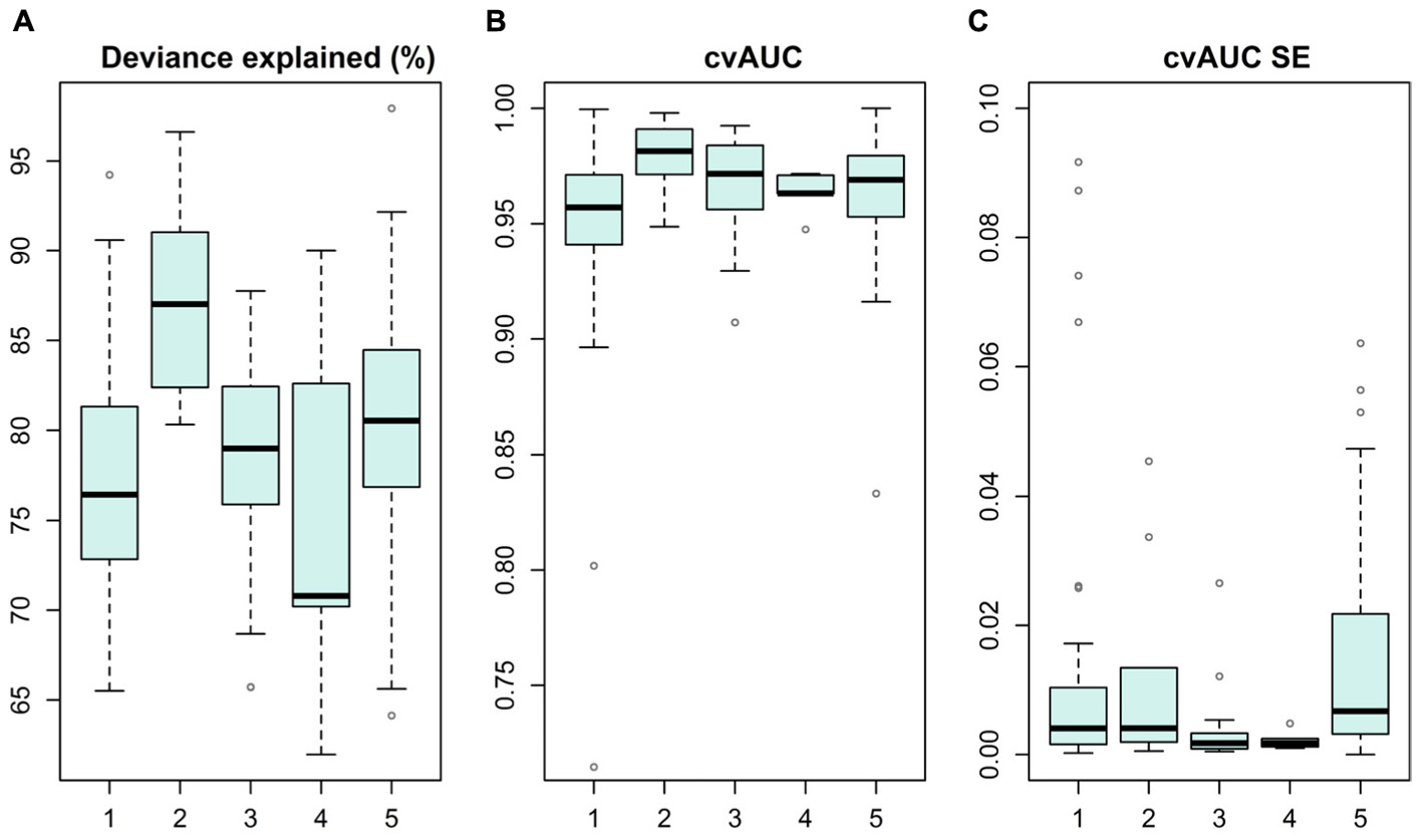
FIGURE 3. Statistical distribution models and their performance reported as deviance explained (%) (A), cross-validated AUC value (B), and standard error for AUC on withheld test data (C). Models are grouped into categories of (1) macroalgae, (2) bryophytes, (3) IUCN Red List of Ecosystems, (4) benthic invertebrates and (5) vascular plants.

Based on the SDMs, habitats and fish reproduction area data, two priority rankings were produced using Zonation (i) an unconstrained “clean slate” solution and (ii) a hierarchical solution constrained by the present MPA network. Figures 4, 5 show the basic Zonation outputs for these analyses; priority rank maps and associated performance curves. These maps summarize a large amount of information useful for marine conservation and marine spatial planning.

FIGURE 4

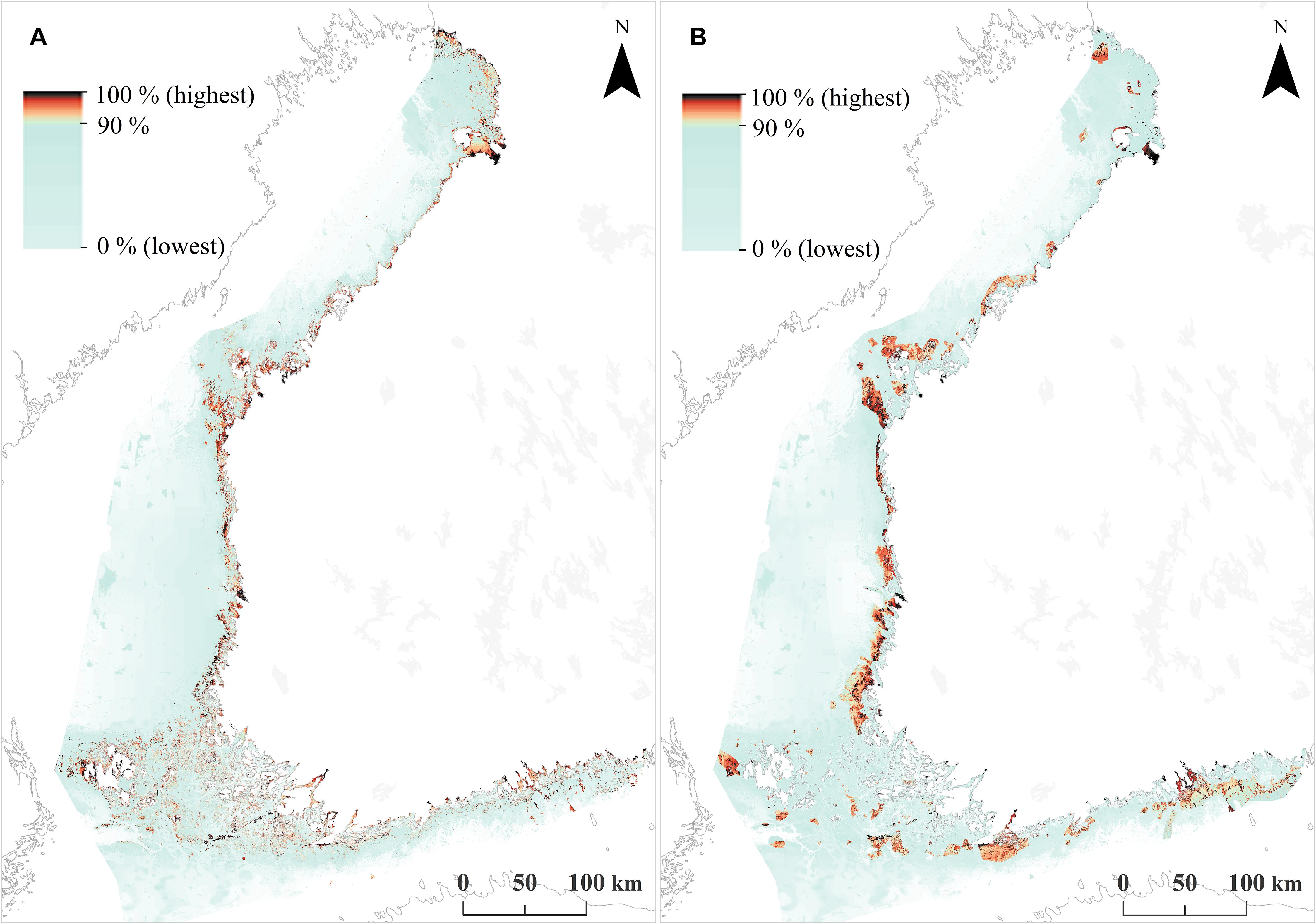
FIGURE 4. Zonation priority rank maps across the Finnish seascape. (A) Unconstrained priority rank map, which corresponds to the establishment of a completely new MPA network. (B) A constrained, hierarchical priority rank map, where the highest priorities are forced inside the present MPA network.

FIGURE 5

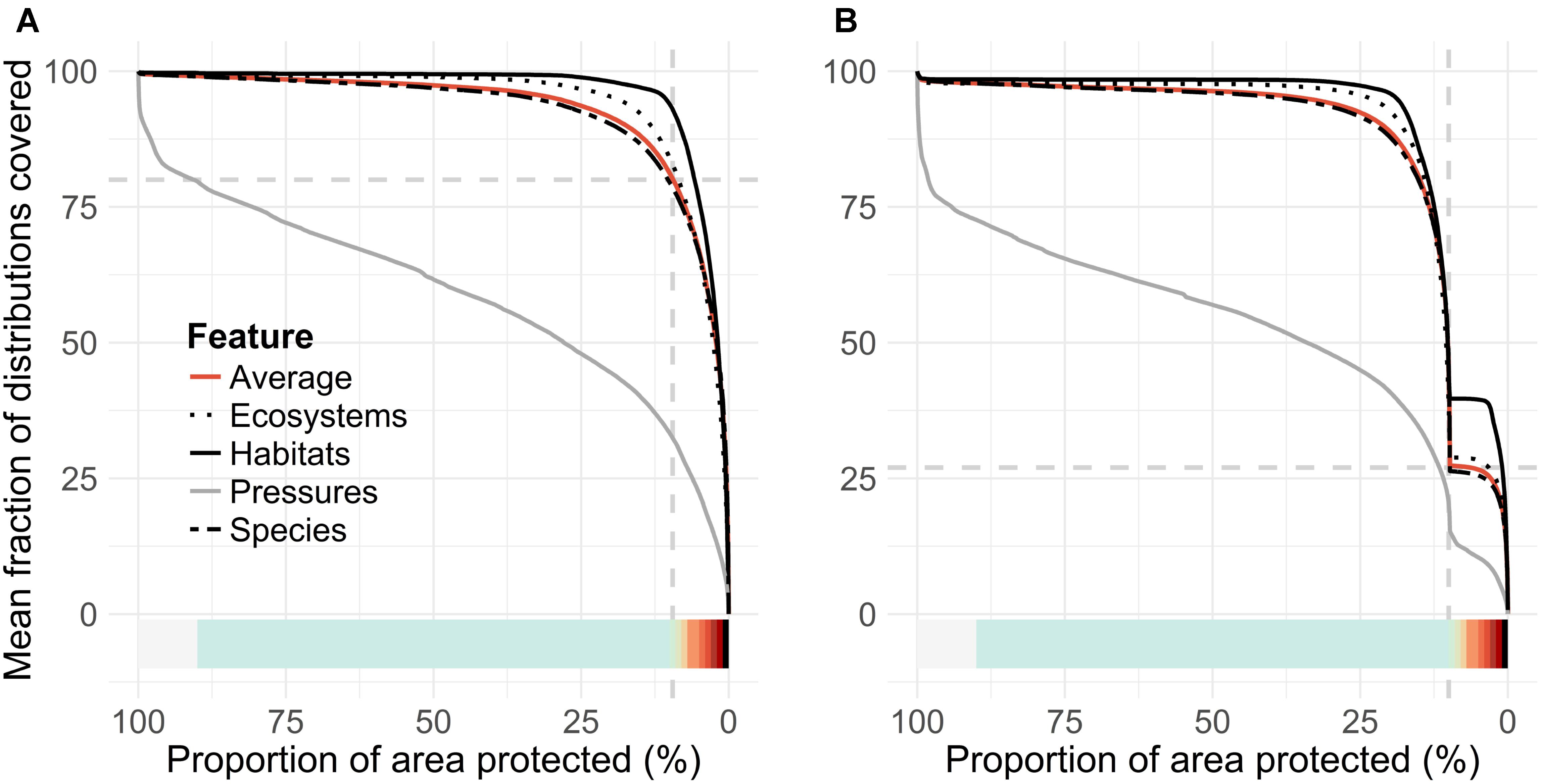
FIGURE 5. Second standard output of a Zonation analysis, performance curves. (A,B) Pair with priority rank maps, Figures 4A,B, respectively, with matching color ramps. These curves summarize mean conservation coverage achieved across groups of features from the respective top-priority areas selected from the priority rank maps. The present MPA network (vertical dashed gray line in both panels) covers 27% (horizontal dashed gray line, B) of the mean conservation coverage, compared to 80% (dashed gray line, A) of the unconstrained Zonation solution.

MPA Network Evaluation and Identification of High-Priority Expansions

The unconstrained priority rank map (Figure 4A) shows where the highest concentrations of marine biodiversity are, when accounting for balance between features. Picking the highest-ranked areas of this map would identify a set of MPAs that would cover conservation value in an area-efficient and balanced manner. As a by-product, the low-ranked areas in this map would be suitable for environmental impact avoidance. However, as MPAs have already been designated, Figure 4B shows a similar result, but from a hierarchical analysis in which the highest priorities are forced inside the existing MPA network. This map allows identification of an ideal expansion for the present MPA network, by picking the highest ranked areas outside the present MPA network. For example, the present Finnish MPA network covers 10% of the seascape, corresponding to the 90–100% top priorities in the hierarchically constrained solution. Consequently, areas ranked from 89–90% would identify an ideal 1% expansion to the present MPA network, areas ranked to 87–90% would identify a 3% expansion, and so on.

The priority rank maps (Figures 4A,B) provide a ranking in which cells are ordered with respect to each other. This ranking does not quantify solution quality in any absolute sense. Thus, the so-called performance curves (Figures 5A,B) are needed. These curves summarize the conservation coverage that would be achieved in any top priority fraction selected from the priority rank maps. Comparison of mean performance curves allows a quick evaluation of the present MPA network. The clearly concave shape of the performance curves (5AC and 5B) tells that marine biodiversity features are, according to the present data, comparatively highly concentrated in the Finnish waters. The present network, which covers 10% of the sea area, covers on average 27% of the distributions of input features (Figure 5B). In comparison, an unconstrained 10% of the seascape could cover 80%, implying that the performance of the present MPA network is mediocre. As a counterpart to comparatively highly concentrated biodiversity, the lowest priority areas (∼80%) include not much biodiversity according to the present data. In general, marine habitats are quite well covered by the MPA network, on average 37% of marine habitats exist within MPAs (cf. the bold black line in Figure 5B).

The quantification of performance shown above (Figures 5A,B) displays only information about average performance across feature groups. Importantly, Zonation outputs also allow investigation of performance for each individual feature. As a summary, Figure 6 shows histograms of fractions of distributions covered across all individual features, for the present MPA network, and expansion by 1, 3, and 5%, starting from the present network, and for the unconstrained analysis solution.

FIGURE 6

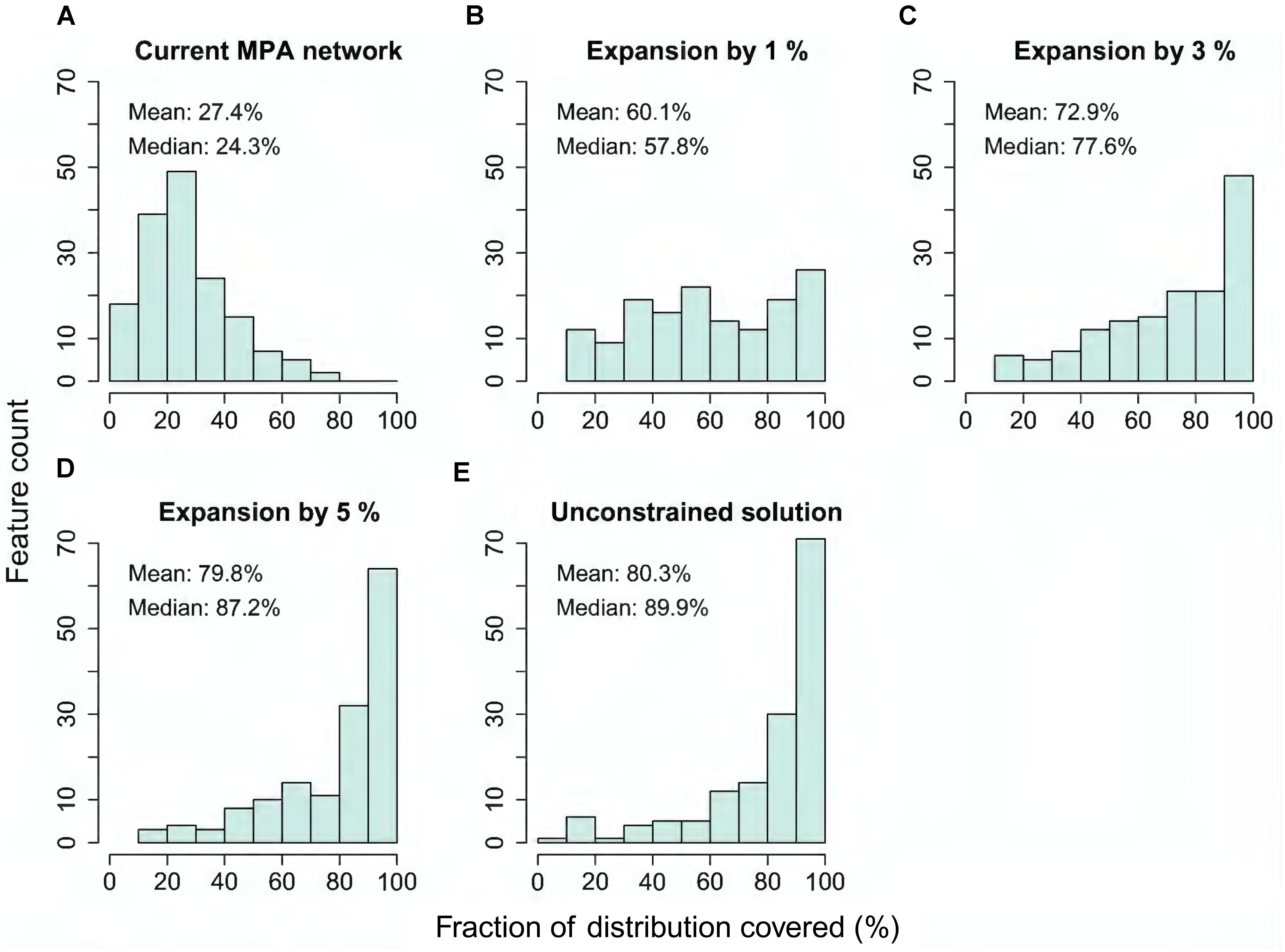
FIGURE 6. (A–E) Histogram of coverage across all input features (excluding marine pressures) when selecting either the present MPA network, plus 1, 3, or 5% area expansions starting from the present network, compared to the ideal solution of the unconstrained analysis. The y-axis of the plot gives the count of features that have conservation coverage according to the bins on the x-axis. For example, the first bin 0–10% gives the count of features that have between zero and 10% of their occurrences covered in the selected set of areas.

Figure 6A shows that the present MPA network is missing an extensive amount of marine biodiversity, and that only a small fraction of features lies within the MPAs. Expansion of the protected area by only one percentage point would introduce a number of (rare and narrowly distributed) species, ecosystems and habitats, such as many brown and red algae, blue mussels, as well as eelgrass beds, which are missing from the present MPA network (Figure 6B and (Supplementary Figure S1). Expansion by 3% (Figure 6C) would further improve the performance and, with an expansion by 5% (4,250 km²), the same conservation level (∼80% of feature distributions) as in the unconstrained MPA network solution (Figure 6E) would be achieved. This result illustrates that well-informed MPA network expansion has potential to significantly increase the ecological performance of the current MPA network.

We evaluated the quality of individual MPAs based on the unconstrained prioritization solution and using the LSM analysis. Generally, the existing MPAs protected marine biodiversity fairly well, as median ranks were above 78% (Figure 7A), with a mean of 87% across MPAs. Still, many MPAs hold only minimal nature values: 5% of the MPAs belong to the lowest 40% of ranks. In general, larger MPAs, such as national parks, hold lower feature densities, whereas Natura 2000 sites, private MPAs and Ramsar sites support significantly higher densities of features (Figure 7B).

FIGURE 7

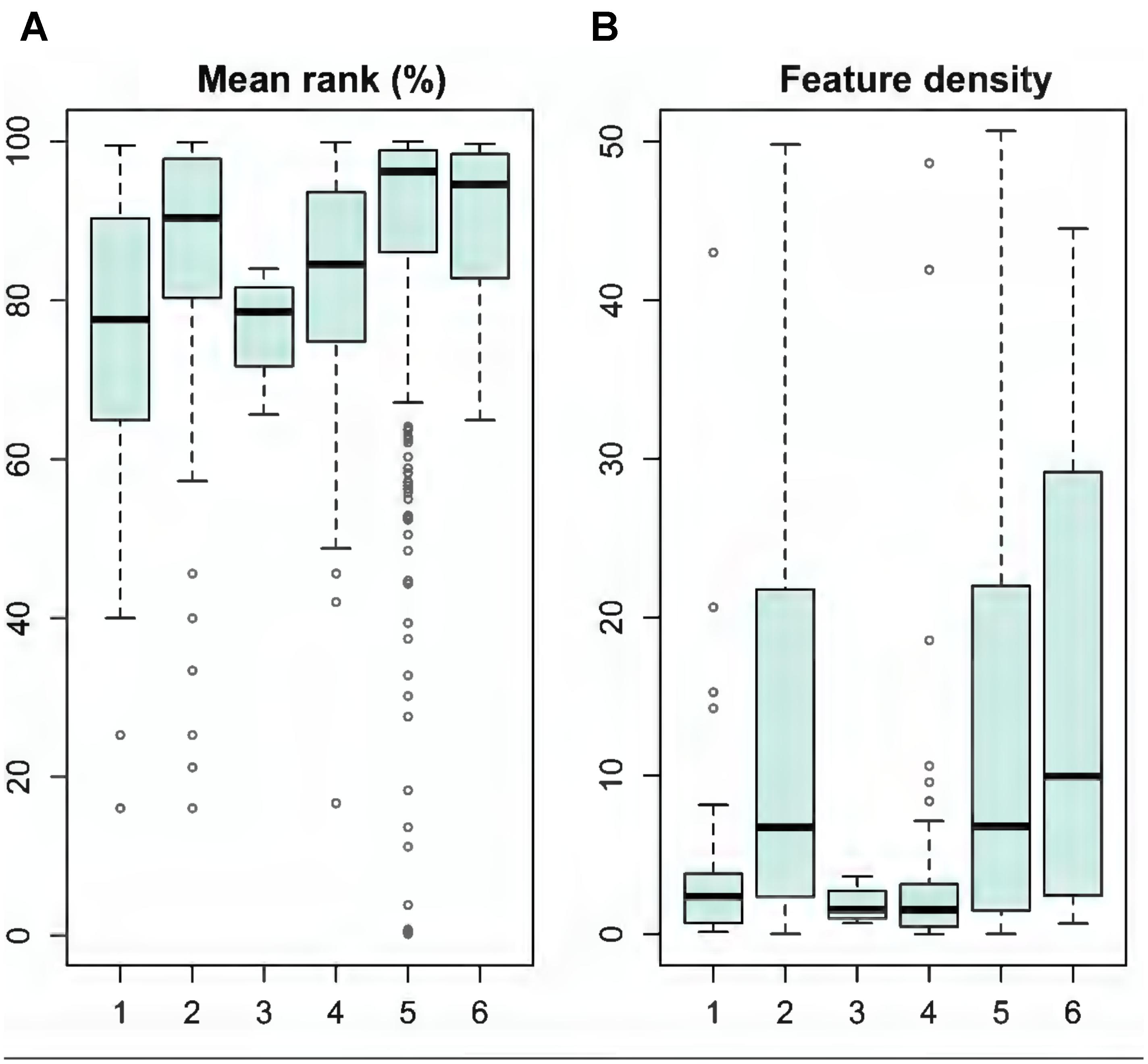
FIGURE 7. Evaluation of the existing MPAs based on data from Landscape Mask (LSM) analysis (see details in section “Analysis Variants and Post-processing”). MPA categories: (1) HELCOM MPAs, (2) Natura 2000 sites, (3) National parks, (4) Nature reserves, (5) Private MPAs, and (6) Ramsar sites. (A) Shows the mean rank (%) of MPAs and (B) feature density of MPAs.

Based on top-priority areas from the constrained analysis, we show in Figure 8 and Table 3 our primary candidates for MPA expansion areas and details of suggestions are shown in (Supplementary Table S2). As habitats are poor surrogates for describing marine biodiversity patterns (see the section “Surrogacy Between Species and Habitats” and Figure 9, below), we also used top priority areas from the species-surrogacy analysis. Suggestions for expansions can be grouped into two major categories: (1) expansions of existing MPAs, areas adjacent to or areas in close proximity of old ones; and (2) independent new MPAs, filling gaps geographically and ecologically, representing regions lacking MPAs, and areas supporting species/marine habitats not covered by the current MPA network. Our illustrative expansion suggestion would increase area protected from the current 10 to 11%, thus increasing the total MPA network area by 850 km². As marine biodiversity is fragmented, and of varying nature from north to south, following mostly the environmental gradient of salinity, our expansion suggestion includes several separate MPAs. In general, new areas are suggested away from pressures, so areas close to cities, harbors or coastal constructions are excluded. MPAs were also not suggested in regions already well protected or holding high conservation priorities fragmented in many small patches.

FIGURE 8

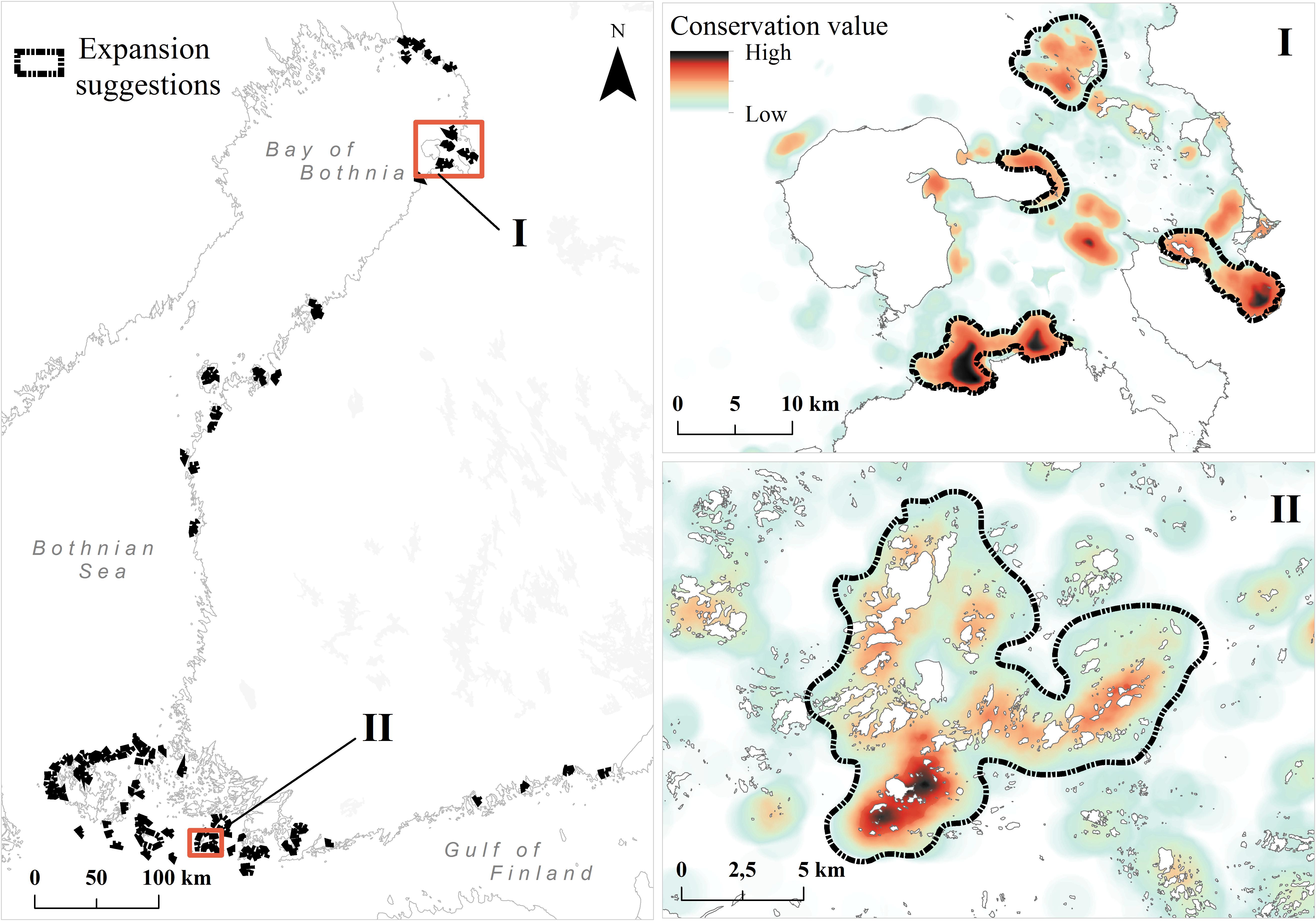
FIGURE 8. Proposed top 3% MPA expansion areas. Suggestions are based on the product of priority ranks and weighted range-size rarity (see details in section “Analysis Variants and Post-processing”). Zoomed-in example images (I and II) are shown from the northern and southern parts of Finnish marine areas. The color ramp in these areas is different from the previous figures; here the ramp shows internal variation inside the top 3% area fraction. Areas of high conservation value inside the present MPAs are not shown.

TABLE 3

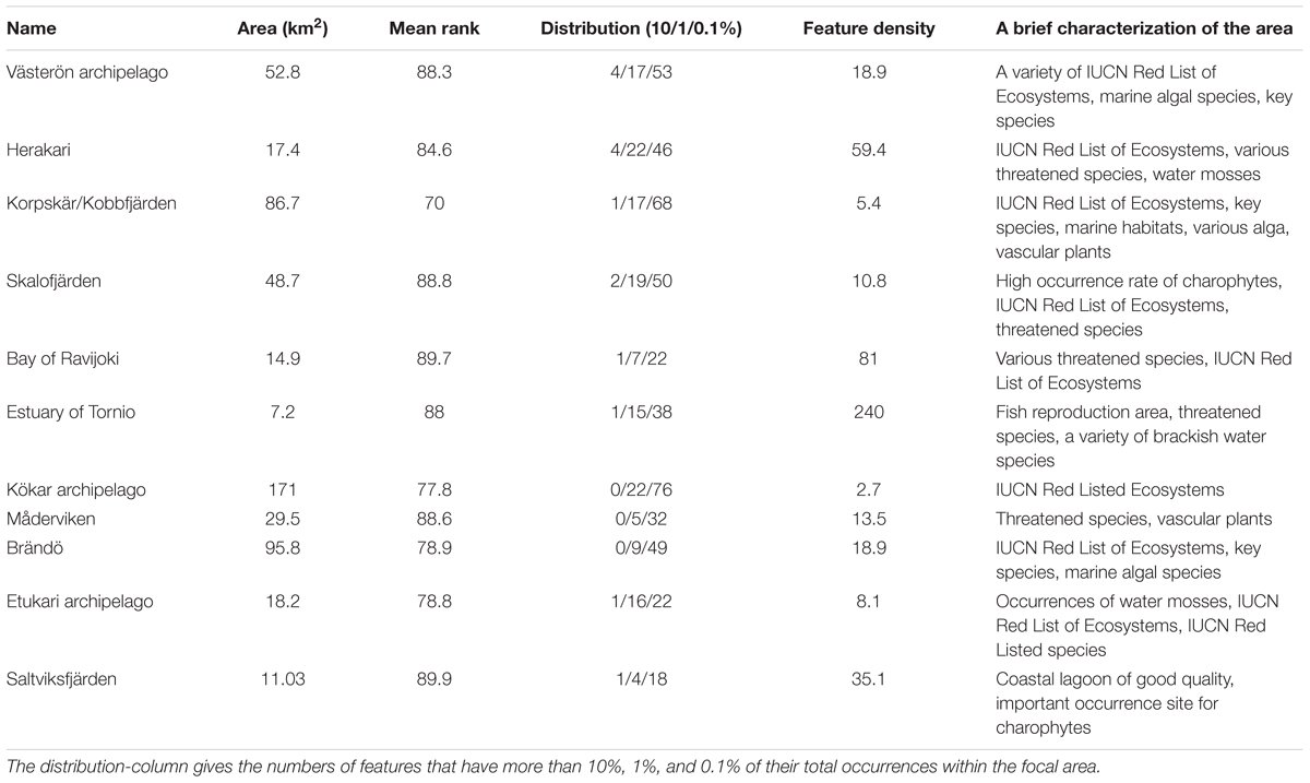
TABLE 3. Characterization of high-quality potential MPA expansion areas, based on mean rank, feature density and area, shown at a random order (full table in Supplementary Material).

FIGURE 9

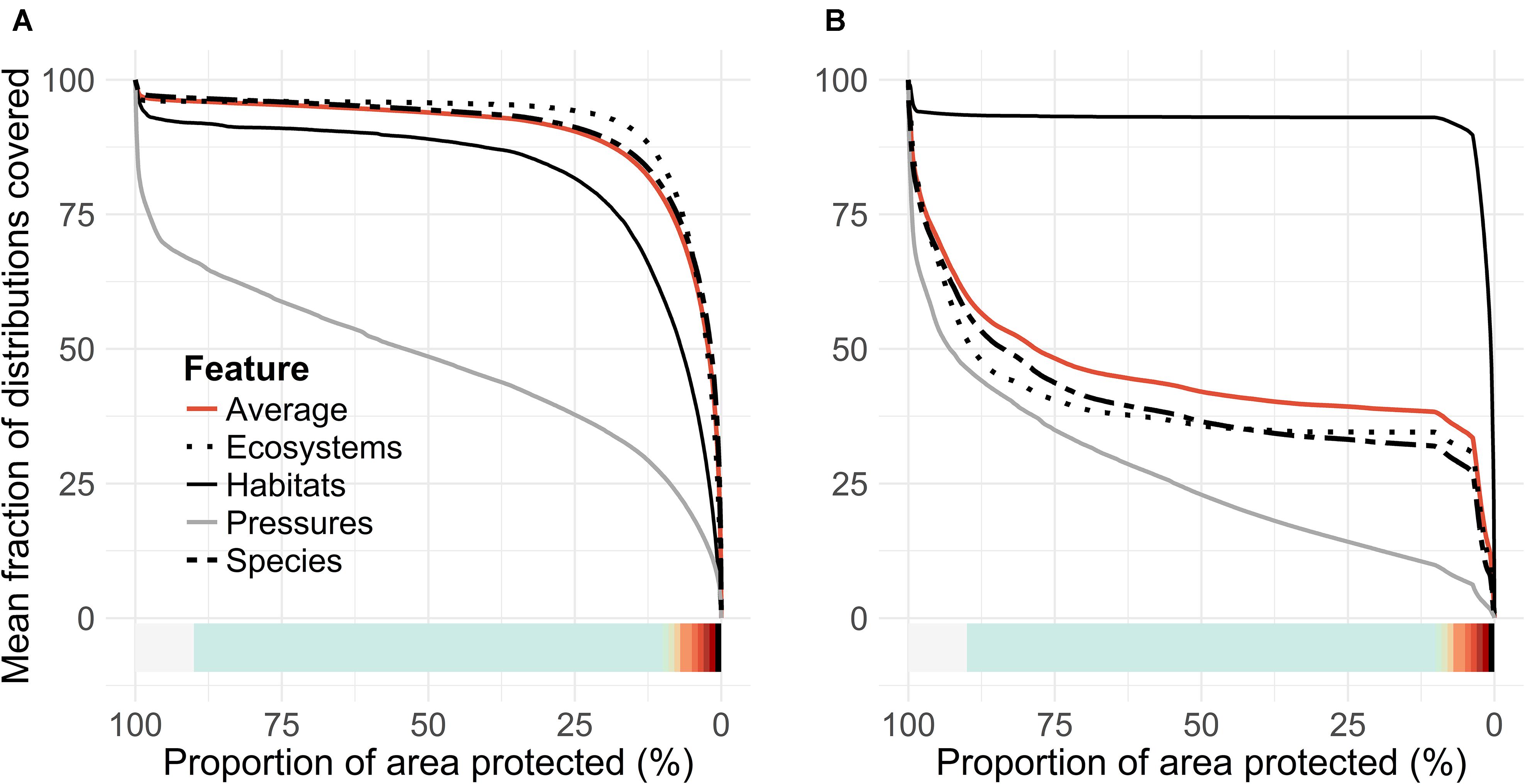
FIGURE 9. Surrogacy of species and marine habitats. (A) Performance curves for analysis driven by species data only and (B) performance curves for analysis driven by habitat data alone.

Our expansion suggestions would increase the conservation level of IUCN Red List of Ecosystems, Red Listed species, threatened species, ecosystem engineers supporting other marine life, and fish reproduction areas. In addition, increases would be achieved in the conservation status of Habitats Directive Annex I habitats (following the guidelines of the Promise of Sydney), and for marine habitats not represented by the Habitats Directive. Table 3 shows the main candidates for expansion areas, based on mean rank, feature density, and the extent of distributions.

Surrogacy Between Species and Habitats

Within the EU, habitats are an accepted basis for MPA design, as much of the knowledge of marine nature in most of the countries relies on information about the locations of marine habitats. We evaluated how well species would act as surrogates for these habitats and how habitats perform as a proxy for species. Figure 9 shows priority rank maps developed based on only habitats (Figure 9A) compared to species-only analysis (Figure 9B). When fractions of distributions covered are evaluated in the species-based analysis, against the one driven by the habitats, it is found that approximately half of the species distributions are lost in the analysis driven by habitats alone. In contrast, when habitat coverage is evaluated from species-only analysis, we find only a minor loss in the average fraction of habitat distributions covered. This means that the species studied act as a good surrogate for marine habitats, but the habitats do not act as good surrogates for species. Note that both species and habitat data were used together to identify our putative MPA network expansions (Figures 4B, 5B).

The mismatch in species surrogacy of habitats can be seen clearly in an example image from the Archipelago Sea (Figure 10). Fragmented bits and pieces of priority habitats are scattered around the seascape (Figure 10B), whereas much of the species-based marine biodiversity is located around the islands, and in the underwater parts of sandy shores (Figure 10A). None of these environments are included in the Finnish interpretation of “reefs” (1170) or “sandbanks which are slightly covered by sea water all the time (1110).

FIGURE 10

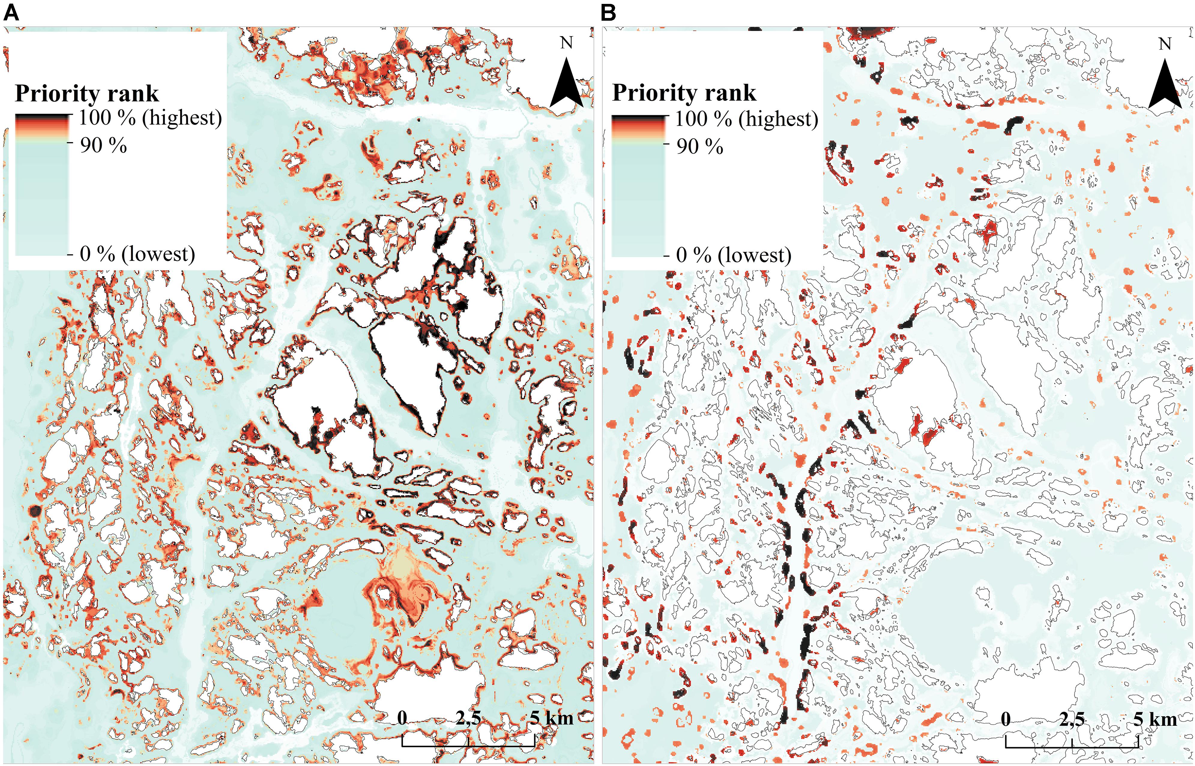
FIGURE 10. Surrogacy analysis priority rank maps in an example area in the Archipelago Sea. (A) Priority rank map based on species data. (B) Priority rank map based on habitat data. Priorities in this region differ substantially between the two analyses. Corresponding performance curves are shown in Figure 9.

Protection Status and Quality of Marine Habitats

The habitats listed in the EU Habitats Directive Annex I cover 6% of the Finnish seascape, and is composed of: 3.2% in Reefs, 0.7% in Boreal Baltic islets, 0.8% in Coastal lagoons, 0.6% in Large shallow inlets and bays, 0.5% in Boreal Baltic narrow inlets, 0.4% in Sand banks, 0.08% in Baltic esker islands, and 0.9% in Estuaries. The existing MPA network protects 24% of Reefs, 32% of Boreal Baltic islets, 18% of Coastal lagoons, 34% of Large shallow inlets and bays, 40% of Boreal Baltic narrow inlets, 49% of Sand banks, 53% of Baltic esker islands, and 21% of Estuaries. Although these habitats are quite well covered by the MPA network, our analysis shows that they miss a large part of functionally important species occurring on rocky and sandy shores, such as major concentrations of brown and red algae, blue mussels and eelgrass. Using the LSM analysis, we assessed how much of the marine biodiversity features each of the habitat types maintain, and how individual habitat patches are ranked in the Zonation constrained solution. Utilizing this information, we were able to identify highly valuable habitat patches outside the current MPA network, and on the other hand evaluate the quality of habitat patches already protected.

Figure 11 shows that there is major variation between habitat patch quality depending on habitat type, whether or not the patch is protected, and patch area. As a general trend, protected habitat patches are of higher quality than unprotected ones. For some habitats, such as coastal lagoons and estuaries, it was possible to find both small and large very high quality unprotected areas (with quality here meaning fractional coverage of distributions of both habitats and species). Feature density is on average larger in smaller (0.16–0.99 km²) habitat patches for Boreal Baltic narrow inlets, Estuaries, and Large shallow inlets and bays, in contrast to Sand banks, Boreal Baltic islets and reefs, where feature densities are lower for smaller areas. For some habitats, such as reefs, it is possible to find high-quality unprotected areas, but only in the smaller patch size.

FIGURE 11

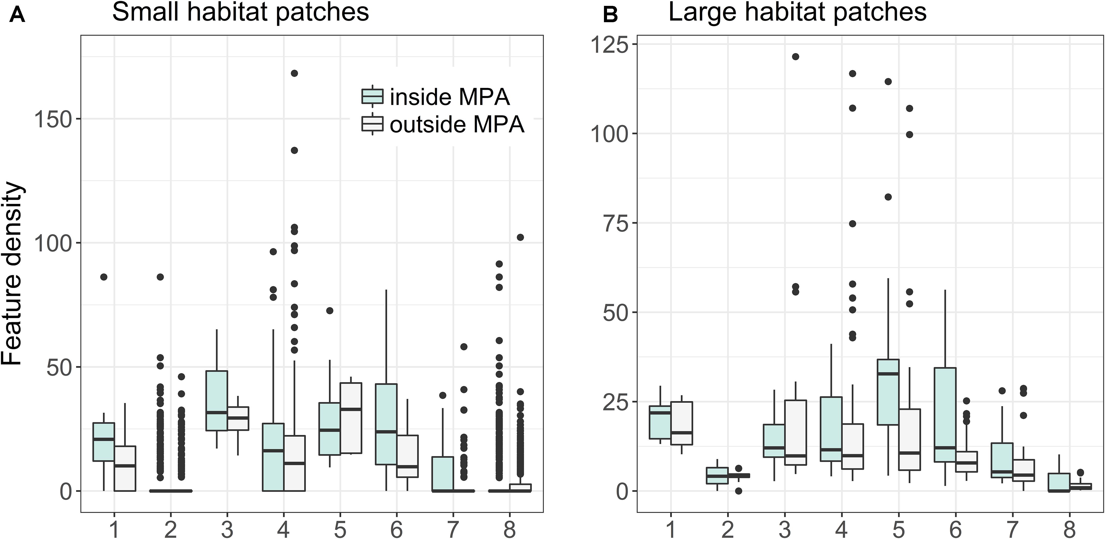
FIGURE 11. Quality of patches of marine habitats based on Zonation LSM-analysis (see details in section “Analysis Variants and Post-processing”). Marine habitats: (1) Baltic esker islands, (2) Boreal Baltic islets, (3) Boreal Baltic narrow inlets, (4) Coastal lagoons, (5) Estuaries, (6) Large shallow inlets and bays, (7) Sand banks, and (8) Reefs. (A,B) Show feature densities for smaller (0.16–0.999 km²) and larger (≥1 km²) habitat patches, respectively.

Discussion

The Finnish Underwater Inventory Programme, VELMU, has taken an unprecedented step forward in the amount and quality of marine data available, even in the global context. Our evaluation of the Finnish MPA network and its expansion was based on a substantial amount of biodiversity data (∼140,000 samples), high-resolution environmental data, and a comprehensive set of analyses, using scientifically established techniques of spatial conservation prioritization (Zonation). Our study revealed that the ecological efficiency of the present Finnish MPA network is mediocre, and it is unbalanced in its coverage of marine biodiversity. This is not surprising, as there was scarce ecological data on marine species and habitats available at the time of the establishment of most of the Finnish MPAs. Protection was based on information on other species, such as seabirds and marine mammals (seals), as well as terrestrial plant species on the islands and skerries. Our approach allowed us to assess the patterns of marine biodiversity features in the Finnish sea area and to evaluate the validity of certain fundamental principles of marine protection, such as usefulness of habitats as surrogates for species.

According to our analyses, marine biodiversity is highly concentrated in the Finnish waters: a smallish fraction (∼22%) of the overall seascape includes more than 91% of the feature coverage. Most of these features occur in relatively shallow and well-lit waters. In contrast, the lowest priority areas, which support little biodiversity, are in the present analysis the deep, dark soft bottom areas, or hypoxic seafloors, and areas with habitat constraints, e.g., harbors. This characterization also applies to the Baltic Sea as a whole. One third of the seafloor is sediment accumulation area in which hypoxia occurs, forming dead zones with little value for biodiversity (Conley et al., 2009; Kaskela et al., 2012; Reusch et al., 2018).

A major finding was that the present MPA network covers only ca. 27% of the distributions of marine biodiversity features. Overall, MPAs protect marine biodiversity, but not adequately. Our analysis shows that the feature coverage could be significantly improved by minor expansion of the protected sea area. Increasing the MPA coverage by just 1%, from 10 to 11% of the seascape, would increase the mean coverage of features from 27 to 60% (Figure 6B). This shows that many species worth conserving have very narrow distributions, and that many key areas for such species are missing from the network. Highest ranked areas outside the present MPA network could fix gaps in conservation, both geographically and ecologically (Table 2). The strong concentration of the biodiversity features is both a benefit and a challenge for conservation. The narrow distribution implies that very small additions in the MPA network are useful. On the other hand, if such areas exist on private waters, or in areas claimed for other human uses, such as aquaculture, energy production or extraction of bottom materials, conflicts between conservation and usage of the sea may arise. If the protection has a scientific definition, rather than a legal basis, the conservation aspects of smallish areas may be neglected in the stakeholder process.

We here focused on searching for individual expansion areas, but Zonation’s post-processing analyses could also be used for identifying connected sets of small areas (skerries, reefs, etc.) that jointly form management landscapes (Moilanen et al., 2005). The priority ranking (Figures 4A,B) has at least two further uses. In addition to identifying areas important for biodiversity conservation, the analysis also identifies areas that are ecologically less important. These low-ranked areas could be suitable for ecological impact avoidance (Kareksela et al., 2013, 2018), for example when planning wind power sites or aquaculture (fish farms). Impact avoidance analyses would benefit from additional data concerning the economic benefits expected from investments in different areas. Combining these economic data with biodiversity data would yield an ecosystem-based and cost-effective solution for placement of human activities in the seascape.

One of the basic demands for an efficient MPA network is that it has adequate representativity. The 2003 World Parks Congress stated that MPAs need to cover at least 20–30% of each marine habitat in order to ensure viability of marine ecosystems (IUCN, 2003). We found that this target has already been reached in Finland for several marine habitats (mentioned in the EU Habitats Directive Annex I). The existing MPA network covers 53% of Baltic esker islands, 49% of sand banks, 40% of Boreal Baltic narrow inlets, 34% of large shallow inlets and bays, 32% of Boreal Baltic islets, 24% of reefs, 21% of estuaries, and 18% of coastal lagoons (Figure 5B). On the other hand, the 20% level is a minimum requirement that refers to strictly protected areas. Much higher levels, up to 50%, are often recommended in scientific studies (e.g., Airamé et al., 2003) and even higher percentages may be needed for, e.g., rare or isolated habitats, and for habitats that form bottleneck areas for reproduction (Roberts et al., 2003). It is notable that the Finnish marine protection is more focused on protecting habitats than rare or functionally important species: the coverages of species, IUCN Red Listed ecosystems and habitats were 26, 28, and 39%, respectively (Figure 5B), but many species have low coverage between 0 and 10% (Figure 6A). We conclude that the representativity of the MPA network could still be improved to better achieve the scientifically accepted conservation objectives.

In areas where the data on species is scarce, the MPAs need to be selected based on information on habitats. This practice is the basis of the EU Habitats Directive, and it is especially important in the northern Baltic, where only a handful of marine species are listed as species requiring protection (cf. EU Habitats Directive Annex II). Many types of habitats common in the European Seas, such as estuaries, large shallow inlets and bays, and coastal lagoons, indeed harbor a large number of species. We however found that – in the Finnish sea area – the habitats listed in the Habitats Directive Annex I act as poor surrogates for species. If only habitat data would be used, approximately 60% smaller coverage of species distributions would be achieved, compared to a situation where features are searched based on both habitats and species (Figure 9). This is at least partly caused by the fact that the extensive shallow water areas surrounding thousands of larger islands are not interpreted as “reefs” (habitat no. 1170 in Habitats Directive) in the Finnish interpretation of the Habitats Directive, neither are they considered together with the habitat “boreal Baltic islets and small islands” (1620). These areas, which may consist of various bottom types from rocky shores to mixed sediments are, according to our prioritization, important biodiversity hotspots, harboring a large number of functionally important species, such as brown, green, and red algae and associated flora and fauna. Similarly, the underwater parts of sandy shores and beaches are not considered to belong to the habitats “sandbanks which are slightly covered with sea water all the time” (1110) or “Baltic esker islands with sandy, rocky and shingle beach vegetation and sublittoral vegetation” (1610). Such environments provide a suitable habitat for various vascular plants and harbor some of the most important occurrences of the keystone species eelgrass (Zostera marina) in Finland. Nevertheless, these areas are not necessarily considered as MPA candidates when marine Natura 2000 areas are designated.

To sum up, habitat maps that rely solely on abiotic surrogates do not function well in describing patterns of biodiversity. Habitats can be abiotically similar but biologically very different, because communities differ along environmental gradients (e.g., salinity), as also concluded in other studies (Stevens and Connolly, 2004; Arponen et al., 2008; Jackson and Lundquist, 2016). We therefore suggest that, to locate and protect hotspots of biological diversity, the interpretations of many of the marine habitats need to be broadened, and a multifaceted basis of protection needs to be adopted. Our analyses of surrogacy also suggest that, in addition to habitats and rare species, also functionally important species should be included in MPA network planning in the Baltic Sea and elsewhere.

We want to emphasize that establishing a sufficient amount of MPAs does not safeguard the integrity of the marine ecosystem. Each of the MPAs also needs to be efficiently managed. Unfortunately, management plans are missing from a large part of the Baltic Sea MPAs (HELCOM, 2010, 2013b), and key restrictions are missing from many areas: e.g., fishing is not restricted in most of the Finnish MPAs. In the future analyses, it will be important to also study the level of protection in respect of the human pressures in the different MPA types. Such an approach will shed more light on the true ecological efficiency of the MPA network.

As always, data quality is a concern in spatial prioritization. Our data about marine biodiversity was of exceptionally wide taxonomic coverage and of high quality, originating from 140,000 standardized VELMU sampling sites. We are not aware of a similar data set elsewhere in the world, where the entire sea area of a nation is covered. Spatial prioritization becomes increasingly stable the more data is driving the analysis (Kujala et al., 2018), and therefore our confidence in the present analysis is high.

There are data that could potentially be used to refine the analysis. Integration of ecosystem services into the present analysis would be useful when planning the MPA networks, because these inform of benefits gained from the ecosystem that otherwise may remain concealed. Also, more detailed information on human pressures could be used, such as inclusion of human activities aiming at conflict resolution between biodiversity conservation and human activities (Moilanen et al., 2011b). This sort of data are not necessarily easy to get, and human pressures tend to shift in space (Joppa et al., 2016). A third major category of data that would improve the MPA network analysis are opportunity costs for alternative sea uses. Inclusion of costs allows identification of cost effective solutions and fair division of costs and benefits between stakeholders. Again, reliable information about opportunity costs is difficult to obtain. It is also notable that we have not considered temporal dimension in our analysis. Species distribution areas may shift for various reasons, including eutrophication and climate change, and human pressures tend to shift in space and time. Forecasting such changes by modeling methods would enable a precautionary approach to MPA network development.

This work illustrates that spatial prioritization applied on high-resolution marine SDMs can support the evaluation and design of MPA networks, and ecosystem-based marine spatial planning. The pre-requisites of such work include (i) broad biodiversity data that ideally covers both habitats and a large array of species, (ii) environmental data at a resolution that allows realistic ecological modeling, and (iii) an analysis path able to utilize these data, such as Zonation. Our approach and methods are applicable to any sea area where these prerequisites are met.

In summary, our analysis included (1) identification of biodiversity hotspots, (2) evaluation of the quality of marine habitats and MPAs, (3) evaluation of the surrogacy of habitats and species, (4) suggested expansion of the protected area network, and (5) an illustrative proposal for new MPA candidates. Our results indicate that, despite reaching the Aichi target 11 (10% of the sea area protected) and the Sydney promise (20 or 30% of habitats protected) the Finnish MPA network does not secure sufficient protection of important biological features of the marine ecosystem. Our approach can be refined and expanded by including various types of additional data (species, ecosystem services, human pressures, opportunity costs etc.) and expansion in space and time of the present work. Especially relevant would be the expansion of this work to the broader Baltic Sea context. Adequate data are not yet available for all countries, but several Baltic Sea countries are currently implementing or starting inventories of varying depth and breadth, allowing production of SDMs for wider areas. This gives hope that in some years’ time a reliable ecological prioritization like the present one would be possible for the entire Baltic Sea.

Author Contributions

EV, AM, and MV designed the study as a whole and designed the spatial prioritization and EV implemented it. EV and JL designed and implemented the distribution modeling. EV wrote the first manuscript, with subsequent contributions from MV, JL, and AM.

Conflict of Interest Statement

The authors declare that the research was conducted in the absence of any commercial or financial relationships that could be construed as a potential conflict of interest.

Acknowledgments

We acknowledge the support from the Academy of Finland Strategic Research Council (project SmartSea, Grant Nos. 292985 and 314225), and the Finnish Inventory Programme for the Underwater Marine Environment (VELMU) and the Finnish Ecological Decision Analysis project (MetZo), both funded by the Ministry of the Environment. We wish to thank the dedicated field staff from several institutes, especially Parks & Wildlife Finland. We wish to acknowledge CSC – IT Center for Science, Finland, for generous computational resources. We thank Tytti Kontula for providing the threat status 2018 report on IUCN Red List Ecosystems, Meri Kallasvuo for providing the fish reproduction area data, Anu Kaskela, Henna Rinne, Matti Sahla, Lasse Kurvinen, and Ville Karvinen for the habitat data, Marco Nurmi for the compilation of human activity data, Kari Kallio and Sofia Junttila for Envisat-MERIS satellite sensor products, and Meri Koskelainen for providing the reed belt data. We thank the two reviewers for insightful comments that significantly improved the manuscript. We thank Husö biological station of Åbo Akademi University for providing Åland islands biological data.

Supplementary Material

The Supplementary Material for this article can be found online at: https://www.frontiersin.org/articles/10.3389/fmars.2018.00402/full#supplementary-material

FIGURE S1 | Coverage of distributions of different subgroups under different priority solutions. Red List of Ecosystems and Habitats, based on threatened status (NT, VU), key species and fish reproduction areas. A is the unconstrained solution (Figure 4A) and B the current MPA network (Figure 4B).

TABLE S1 | Species observed in the VELMU programme 2004-2016 from dives and videos, observation thresholds of species included in the model iterations, and a weighting group where each species belongs to (highest weighting criteria reported. If species belongs to another weighting group, the weights have been balanced accordingly).

TABLE S2 | MPA expansion suggestions reported at a random order, based on mean rank, feature density and size.

References

Agardy, T., di Sciara, G. N., and Christie, P. (2011). Mind the gap addressing the shortcomings of marine protected areas through large scale marine spatial planning. Mar. Policy 35, 226–232. doi: 10.1016/j.marpol.2010.10.006

CrossRef Full Text | Google Scholar

Airamé, S., Dugan, J. E., Lafferty, K. D., Leslie, H., McArdle, D. A., and Warner, R. R. (2003). Applying ecological criteria to marine reserve design: a case study from the california channel islands. Ecol. Appl. 13, 170–184. doi: 10.1890/1051-0761(2003)013[0170:AECTMR]2.0.CO;2

CrossRef Full Text

Arponen, A., Moilanen, A., and Ferrier, S. (2008). A successful community-level strategy for conservation prioritization. J. Appl. Ecol. 45, 1436–1445. doi: 10.1111/j.1365-2664.2008.01513.x

CrossRef Full Text | Google Scholar

Bekkby, T., Isachsen, P. E., Isaeus, M., and Bakkestuen, V. (2008). GIS modeling of wave exposure at the seabed: a depth-attenuated wave exposure model. Mar. Geod. 31, 117–127. doi: 10.1080/01490410802053674

CrossRef Full Text | Google Scholar

Bonsdorff, E. (2006). Zoobenthic diversity-gradients in the Baltic Sea: continuous post-glacial succession in a stressed ecosystem. J. Exp. Mar. Biol. Ecol. 330, 383–391. doi: 10.1016/j.jembe.2005.12.041

CrossRef Full Text | Google Scholar

Breiner, F. T., Guisan, A., Bergamini, A., and Nobis, M. P. (2015). Overcoming limitations of modelling rare species by using ensembles of small models. Methods Ecol. Evol. 6, 1210–1218. doi: 10.1111/2041-210X.12403

CrossRef Full Text | Google Scholar

Breiner, F. T., Nobis, M. P., Bergamini, A., and Guisan, A. (2018). Optimizing ensembles of small models for predicting the distribution of species with few occurrences. Methods Ecol. Evol. 9, 802–808. doi: 10.1111/2041-210X.12957

CrossRef Full Text | Google Scholar

CBD (2004) Decisions Adopted by the Conference of the Parties to the Convention on Biological Diversity at its Seventh Meeting. Rio de Janeiro: Convention on Biological Diversity (COP 7). UNEP/CBD/COP/7/21.

Google Scholar

CBD (2010) Aichi Biodiversity Targets. Convention on Biological Diversity. Available at: https://www.cbd.int/sp/targets/ [accessed April 23, 2018].

Conley, D. J., Carstensen, J., Vaquer-Sunyer, R., and Duarte, C. M. (2009). Ecosystem thresholds with hypoxia. Hydrobiologia 207, 21–29. doi: 10.1007/s10750-009-9764-2

CrossRef Full Text | Google Scholar

De’ath, G., and Fabricius, K. E. (2000). Classification and regression trees: a powerful yet simple technique for ecological data analysis. Ecology 81, 3178–3192. doi: 10.1890/0012-9658(2000)081[3178:CARTAP]2.0.CO;2

CrossRef Full Text

Di Minin, E., Soutullo, A., Bartesaghi, L., Rios, M., Szephegyi, M. N., and Moilanen, A. (2017). Integrating biodiversity, ecosystem services and socio-economic data to identify priority areas and landowners for conservation actions at the national scale. Biol. Conserv. 206, 56–64. doi: 10.1016/j.biocon.2016.11.037

CrossRef Full Text | Google Scholar

Di Minin, E., Veach, V., Lehtomäki, J., Montesino Pouzols, F., and Moilanen, A. (2014). A Quick Introduction to Zonation. Helsinki: University of Helsinki.

Google Scholar

Directive, E. (2008). 56/EC of the European parliament and of the Council of 17 June 2008 establishing a framework for community action in the field of marine environmental policy (Marine Strategy Framework Directive). Offic. J. Eur. Union 164, 19–40.

Google Scholar

EC (1992). Council directive 92/43/EEC of 21 May 1992 on the conservation of natural habitats and of wild fauna and flora. Offic. J. Lett. 206, 7–50.

Google Scholar

Edgar, G. J., Stuart-Smith, R. D., Willis, T. J., Kininmonth, S., Baker, S. C., Banks, S., et al. (2014). Global conservation outcomes depend on marine protected areas with five key features. Nature 506, 216–220. doi: 10.1038/nature13022

PubMed Abstract | CrossRef Full Text | Google Scholar

EEA (2013). Reporting Under Article 17 of the Habitats Directive (period 2007-2012). Available at: https://bd.eionet.europa.eu/activities/Reporting/Article_17 [accessed April 23, 2018].

Google Scholar

EEA (2015) Marine protected areas in Europe’s seas – An overview and perspectives for the future: EEA Report No 3/2015. København: European Environment Agency.

Elith, J., Kearney, M., and Phillips, S. (2010). The art of modelling range-shifting species. Methods Ecol. Evol. 1, 330–342. doi: 10.1111/j.2041-210X.2010.00036.x

CrossRef Full Text | Google Scholar

Elith, J., and Leathwick, J. R. (2009). Species distribution models: ecological explanation and prediction across space and time. Ann. Rev. Ecol. Evol. Syst. 40, 677–697. doi: 10.1146/annurev.ecolsys.110308.120159

CrossRef Full Text | Google Scholar

Elith, J., Leathwick, J. R., and Hastie, T. (2008). A working guide to boosted regression trees. J. Anim. Ecol. 77, 802–813. doi: 10.1111/j.1365-2656.2008.01390.x

PubMed Abstract | CrossRef Full Text | Google Scholar

Elsäßer, B., Fariñas-Franco, J. M., Wilson, C. D., Kregting, L., and Roberts, D. (2013). Identifying optimal sites for natural recovery and restoration of impacted biogenic habitats in a special area of conservation using hydrodynamic and habitat suitability modelling. J. Sea Res. 77, 11–21. doi: 10.1016/j.seares.2012.12.006

CrossRef Full Text | Google Scholar

Evans, D. (2012). Building the European union’s natura 2000 network. Nat. Conserv. 1, 11–26. doi: 10.3897/natureconservation.1.1808

CrossRef Full Text | Google Scholar

Fariñas-Franco, J. M., Pearce, B., Mair, J. M., Harries, D. B., MacPherson, R. C., Porter, J. S., et al. (2018). Missing native oyster (Ostrea edulis L.) beds in a European Marine Protected Area: Should there be widespread restorative management? Biol. Conserv. 221, 293–311. doi: 10.1016/j.biocon.2018.03.010

CrossRef Full Text | Google Scholar

Foster, N. L., Rees, S., Langmead, O., Griffiths, C., Oates, J., and Attrill, M. J. (2017). Assessing the ecological coherence of a marine protected area network in the Celtic Seas. Ecosphere 8:e01688. doi: 10.1002/ecs2.1688

CrossRef Full Text | Google Scholar

Gill, D. A., Mascia, M. B., Ahmadia, G. N., Glew, L., Lester, S. E., Barnes, M., et al. (2017). Capacity shortfalls hinder the performance of marine protected areas globally. Nature 543, 665–669. doi: 10.1038/nature21708

PubMed Abstract | CrossRef Full Text | Google Scholar

Gormley, K. S. G., Porter, J. S., Bell, M. C., Hull, A. D., and Sanderson, W. G. (2013). Predictive habitat modelling as a tool to assess the change in distribution and extent of an OSPAR priority habitat under an increased ocean temperature scenario: consequences for marine protected area networks and management. PLoS One 8:e68263. doi: 10.1371/journal.pone.0068263

PubMed Abstract | CrossRef Full Text | Google Scholar

Halpern, B. S. (2014). Conservation: making marine protected areas work. Nature 506, 167–168. doi: 10.1038/nature13053

PubMed Abstract | CrossRef Full Text | Google Scholar

Halpern, B. S., Longo, C., Lowndes, J. S. S., Best, B. D., Frazier, M., Katona, S. K., et al. (2015). Patterns and Emerging Trends in Global Ocean Health. PLoS One 10:e0117863. doi: 10.1371/journal.pone.0117863

PubMed Abstract | CrossRef Full Text | Google Scholar

Halpern, B. S., Walbridge, S., Selkoe, K. A., Kappel, C. V., Micheli, F., Agrosa, C., et al. (2008). A global map of human impact on marine ecosystems. Science 319:948. doi: 10.1126/science.1149345

PubMed Abstract | CrossRef Full Text | Google Scholar

Halpern, B. S., and Warner, R. R. (2002). Marine reserves have rapid and lasting effects. Ecol. Lett. 5, 361–366. doi: 10.1046/j.1461-0248.2002.00326.x

CrossRef Full Text | Google Scholar

Hanski, I. (2011). Habitat loss, the dynamics of biodiversity, and a perspective on conservation. Ambio 40, 248–255. doi: 10.1007/s13280-011-0147-3

PubMed Abstract | CrossRef Full Text | Google Scholar

Hastie, T., Tibshirani, R., and Friedman, J. H. (2001). The Elements of Statistical Learning: Data Mining, Inference, and Prediction. New York, NY: Springer-Verlag. doi: 10.1007/978-0-387-21606-5

CrossRef Full Text | Google Scholar

HELCOM (2012). “Checklist of baltic sea macro-species,” in Baltic Sea Environment Proceedings No. 130 (Helsinki: Helsinki Commission).

Google Scholar

HELCOM (2013a). “HELCOM red list of baltic sea species in danger of becoming extinct,” in Baltic Sea Environment Proceedings No 140 (Helsinki: Helsinki Commission).

Google Scholar

HELCOM (2010). “Towards an ecologically coherent network of well-managed Marine protected areas – Implementation report on the status and ecological coherence of the HELCOM BSPA network: Executive Summary,” in Baltic Sea Environment Proceedings No 124A (Helsinki: Helsinki Commission).

HELCOM (2013b). “HELCOM PROTECT – Overview of the status of the network of Baltic Sea MPAs,” in Baltic Marine Environment Protection Commission (Helsinki: Helsinki Commission), 31.

Howell, L. K., Piechaud, N., Downie, A. -L., and Kenny, A. (2016). The distribution of deep-sea sponge aggregations in the North Atlantic and implications for their effective spatial management. Deep Sea Res. Part I: Oceanogr. Res. Papers 115, 309–320. doi: 10.1016/j.dsr.2016.07.005

CrossRef Full Text | Google Scholar

IUCN (2003). Recommendation 5.22, 5th IUCN World Parks Congress, Durban, South Africa (8-17th September, 2003). Available at: www.iucn.org/themes/wcpa/wpc2003/pdfs/outputs/recommendations/approved/english/html/r22.htm (accessed July 08, 2018).

Jackson, S. E., and Lundquist, C. J. (2016). Limitations of biophysical habitats as biodiversity surrogates in the Hauraki Gulf Marine Park. Pacific Conserv. Biol. 22, 159–172. doi: 10.1071/PC15050

CrossRef Full Text | Google Scholar

Jameson, S. C., Tupper, M. H., and Ridley, J. M. (2002). The three screen doors: can marine “protected” areas be effective? Mar. Pollut. Bull. 44, 1177–1183. doi: 10.1016/S0025-326X(02)00258-8

PubMed Abstract | CrossRef Full Text | Google Scholar

Jiménez-Valverde, A., and Lobo, J. M. (2007). Threshold criteria for conversion of probability of species presence to either–or presence–absence. Acta Oecol. 31, 361–369. doi: 10.1016/j.actao.2007.02.001

CrossRef Full Text | Google Scholar

Jonsson, P. R., Kotta, J., Andersson, H. C., Herkül, K., Virtanen, E., Nyström Sandman, A., and Johannesson, K. (2018) High climate velocity and population fragmentation may constrain climate-driven range shift of the key habitat former Fucus vesiculosus in the Baltic Sea. Divers. Distribut. 24, 892–905. doi: 10.1111/ddi.12733

CrossRef Full Text

Joppa, L. N., Connor, B., Visconti, P., Smith, C., Geldmann, J., Hoffmann, M., et al. (2016). Filling in biodiversity threat gaps. Science 352:416. doi: 10.1126/science.aaf3565

PubMed Abstract | CrossRef Full Text | Google Scholar

Kallasvuo, M., Vanhatalo, J., and Veneranta, L. (2016). Modeling the spatial distribution of larval fish abundance provides essential information for management. Can. J. Fish. Aquat. Sci. 74, 636–649. doi: 10.1139/cjfas-2016-0008

CrossRef Full Text | Google Scholar

Kareksela, S., Moilanen, A., Ristaniemi, O., Välivaara, R., and Kotiaho, J. S. (2018). Exposing ecological and economic costs of the research-implementation gap and compromises in decision making. Conserv. Biol. 32, 9–17. doi: 10.1111/cobi.13054

PubMed Abstract | CrossRef Full Text | Google Scholar

Kareksela, S., Moilanen, A., Tuominen, S., and Kotiaho, J. S. (2013). Use of inverse spatial conservation prioritization to avoid biological diversity loss outside protected areas. Conserv. Biol. 27, 1294–1303. doi: 10.1111/cobi.12146

PubMed Abstract | CrossRef Full Text | Google Scholar

Kaskela, A., and Rinne, H. (2018). Vedenalaisten Natura -Luontotyyppien Mallinnus Suomen Merialueella: Tutkimustyöraportti. Espoo: Geologian tutkimuskeskus.

Kaskela, A. M., Kotilainen, A. T., Al-Hamdani, Z., Leth, J. O., and Reker, J. (2012). Seabed geomorphic features in a glaciated shelf of the Baltic Sea. Estuarine Coastal Shelf Sci. 100, 150–161. doi: 10.1016/j.ecss.2012.01.008

CrossRef Full Text | Google Scholar

Kremen, C., Cameron, A., Moilanen, A., Phillips, S. J., Thomas, C. D., Beentje, H., et al. (2008). Aligning conservation priorities across taxa in madagascar with high-resolution planning tools. Science 320:222. doi: 10.1126/science.1155193

PubMed Abstract | CrossRef Full Text | Google Scholar

Kujala, H., Moilanen, A., and Gordon, A. (2018). Spatial characteristics of species distributions as drivers in conservation prioritization. Methods Ecol. Evol. 9, 1121–1132. doi: 10.1111/2041-210X.12939

CrossRef Full Text | Google Scholar

Leathwick, J., Moilanen, A., Francis, M., Elith, J., Taylor, P., Julian, K., et al. (2008). Novel methods for the design and evaluation of marine protected areas in offshore waters. Conserv. Lett. 1, 91–102. doi: 10.1111/j.1755-263X.2008.00012.x

CrossRef Full Text | Google Scholar

Lehtomaki, J., and Moilanen, A. (2013). Methods and workflow for spatial conservation prioritization using Zonation. Environ. Modell. Softw. 47, 128–137. doi: 10.1016/j.envsoft.2013.05.001

CrossRef Full Text | Google Scholar

Lehtomäki, J., Tomppo, E., Kuokkanen, P., Hanski, I., and Moilanen, A. (2009). Applying spatial conservation prioritization software and high-resolution GIS data to a national-scale study in forest conservation. For. Ecol. Manage. 258, 2439–2449. doi: 10.1016/j.foreco.2009.08.026

CrossRef Full Text | Google Scholar

Lester, S. E., Halpern, B. S., Grorud-Colvert, K., Lubchenco, J., Ruttenberg, B. I., Gaines, S. D., et al. (2009). Biological effects within no-take marine reserves: a global synthesis. Mar. Ecol. Progr. Ser. 384, 33–46. doi: 10.3354/meps08029

CrossRef Full Text | Google Scholar

Mikkonen, N., and Moilanen, A. (2013). Identification of top priority areas and management landscapes from a national Natura 2000 network. Environ. Sci. Policy 27, 11–20. doi: 10.1016/j.envsci.2012.10.022

CrossRef Full Text | Google Scholar

Moilanen, A. (2007). Landscape zonation, benefit functions and target-based planning: unifying reserve selection strategies. Biol. Conserv. 134, 571–579. doi: 10.1016/j.biocon.2006.09.008

CrossRef Full Text | Google Scholar

Moilanen, A., Franco, A. M. A., Early, R. I., Fox, R., Wintle, B., and Thomas, C. D. (2005). Prioritizing multiple-use landscapes for conservation: methods for large multi-species planning problems. Proc. R. Soc. B-Biol. Sci. 272, 1885–1891. doi: 10.1098/rspb.2005.3164

PubMed Abstract | CrossRef Full Text | Google Scholar

Moilanen, A., and Kujala, H. (2014). Zonation Spatial Conservation Planning Framework and Software v. 4.0, User Manual. Helsinki: University of Helsinki,

Google Scholar

Moilanen, A., Leathwick, J. R., and Quinn, J. M. (2011a). Spatial prioritization of conservation management. Conserv. Lett. 4, 383–393. doi: 10.1111/j.1755-263X.2011.00190.x

CrossRef Full Text | Google Scholar

Moilanen, A., Anderson, B. J., Eigenbrod, F., Heinemeyer, A., Roy, D. B., Gillings, S., et al. (2011b). Balancing alternative land uses in conservation prioritization. Ecol. Appl. 21, 1419–1426. doi: 10.1890/10-1865.1

PubMed Abstract | CrossRef Full Text | Google Scholar

MPAtlas (2018) Atlas of Marine Protection. Country Summary: Finland. Available at: http://www.mpatlas.org/region/country/FIN/ (accessed April 23, 2018).

Ojaveer, H., Jaanus, A., MacKenzie, B. R., Martin, G., Olenin, S., Radziejewska, T., et al. (2010). Status of biodiversity in the Baltic Sea. PLoS One 5:e12467. doi: 10.1371/journal.pone.0012467

PubMed Abstract | CrossRef Full Text | Google Scholar

Olsen, E. M., Johnson, D., Weaver, P., Goñi, R., Ribeiro, M.C., Rabaut, M., et al. (2013). Achieving Ecologically Coherent MPA Networks in Europe: Science Needs and Priorities. Marine Board Position Paper 18. Ostend: European Marine Board.

Google Scholar

Pouzols, F. M., Toivonen, T., Di Minin, E., Kukkala, A. S., Kullberg, P., Kuustera, J., et al. (2014). Global protected area expansion is compromised by projected land-use and parochialism. Nature 516, 383–386. doi: 10.1038/nature14032

PubMed Abstract | CrossRef Full Text | Google Scholar

R Core Team (2017). R: A Language and Environment for Statistical Computing. Vienna: R Foundation for Statistical Computing.

Google Scholar

Reusch, T. B. H., Dierking, J., Andersson, H. C., Bonsdorff, E., Carstensen, J., Casini, M., et al. (2018). The Baltic Sea as a time machine for the future coastal ocean. Sci. Adv. 4:eaar8195.

PubMed Abstract | Google Scholar

Rinne, H., Kaskela, A., Downie, A. L., Tolvanen, H., von Numers, M., and Mattila, J. (2014). Predicting the occurrence of rocky reefs in a heterogeneous archipelago area with limited data. Estuar. Coastal Shelf Sci. 138, 90–100. doi: 10.1016/j.ecss.2013.12.025

CrossRef Full Text | Google Scholar

Roberts, C. M., Branch, G., Bustamante, R. H., Castilla, J. C., Dugan, J., Halpern, B. S., et al. (2003). Application of ecological criteria in selecting marine reserves and developing reserve networks. Ecol. Appl. 13, 215–228. doi: 10.1890/1051-0761(2003)013[0215:AOECIS]2.0.CO;2

CrossRef Full Text

Robinson, L. M., Elith, J., Hobday, A. J., Pearson, R. G., Kendall, B. E., Possingham, H. P., et al. (2011). Pushing the limits in marine species distribution modelling: lessons from the land present challenges and opportunities. Global Ecol. Biogeogr. 20, 789–802. doi: 10.1111/j.1466-8238.2010.00636.x

CrossRef Full Text | Google Scholar

Sala, E., Lubchenco, J., Grorud-Colvert, K., Novelli, C., Roberts, C., and Sumaila, U. R. (2018). Assessing real progress towards effective ocean protection. Mar. Policy 91, 11–13. doi: 10.1016/j.marpol.2018.02.004

CrossRef Full Text | Google Scholar

Schapire, R. (2003) “The boosting approach to machine learning – An overview,” in MSRI Workshop on Nonlinear Estimation and Classification, 2002, eds. D. Denison, M. H. Hansen, C. Holmes, B. Mallick and Y. Yu (New York, NY: Springer). doi: 10.1007/978-0-387-21579-2_9

CrossRef Full Text | Google Scholar

Stevens, T., and Connolly, R. M. (2004). Testing the utility of abiotic surrogates for marine habitat mapping at scales relevant to management. Biol. Conserv. 119, 351–362. doi: 10.1016/j.biocon.2003.12.001

CrossRef Full Text | Google Scholar

Sundblad, G., and Bergström, U. (2014). Shoreline development and degradation of coastal fish reproduction habitats. Ambio 43, 1020–1028. doi: 10.1007/s13280-014-0522-y

PubMed Abstract | CrossRef Full Text | Google Scholar

Sundblad, G., Bergstrom, U., and Sandstrom, A. (2011). Ecological coherence of marine protected area networks: a spatial assessment using species distribution models. J. Appl. Ecol. 48, 112–120. doi: 10.1111/j.1365-2664.2010.01892.x

CrossRef Full Text | Google Scholar

Viitasalo, M., Kostamo, K., Hallanaro, E.-L., Viljanmaa, W., Kiviluoto, S., Ekebom, J., et al. (eds.) (2017) Meren Aarteet. Helsinki: Gaudeamus.

Wenzel, L., Laffoley, D., Caillaud, A., and Zuccarino-Crowe, C. (2016). Protecting the world’s ocean – The promise of sydney. Aquat. Conserv. Mar. Freshw. Ecosyst. 26, 251–255. doi: 10.1002/aqc.2659

CrossRef Full Text | Google Scholar

Wilson, C. D., Roberts, D., and Reid, N. (2011). Applying species distribution modelling to identify areas of high conservation value for endangered species: a case study using Margaritifera margaritifera (L.). Biol. Conserv. 144, 821–829. doi: 10.1016/j.biocon.2010.11.014

CrossRef Full Text | Google Scholar

Worm, B., Barbier, E., Beaumont, N., Duffy, J., Folke, C., Halpern, B., et al. (2006). Impacts of biodiversity loss on ocean ecosystem services. Science 314, 787–790. doi: 10.1126/science.1132294

PubMed Abstract | CrossRef Full Text | Google Scholar

Zettler, M. L., Karlsson, A., Kontula, T., Gruszka, P., Laine, A. O., Herkül, K., et al. (2014). Biodiversity gradient in the Baltic Sea: a comprehensive inventory of macrozoobenthos data. Helgol. Mar. Res. 68, 49–57. doi: 10.1007/s10152-013-0368-x

CrossRef Full Text | Google Scholar