The Effect of Optical Properties on Secchi Depth and Implications for Eutrophication Management

Introduction

Human activities have increased the transport of nutrients and organic matter from land to coastal waters, often resulting in eutrophication (Nixon, 1995). Eutrophication increases phytoplankton biomass and the chlorophyll-a concentration (Chl-a) decreases light availability for benthic vegetation (Nixon, 1995), and—if severe—can deplete oxygen near the sea bottoms with fatal effects on benthic fauna (Diaz and Rosenberg, 2008). In the Baltic Sea, eutrophication is one of the main challenges for good water quality (HELCOM, 2009; Jutterström et al., 2014) and several international agreements and programs are in place in order to mitigate the negative effects. The EU Water Framework Directive (WFD) focuses on the coastal zone, while the EU Marine Strategy Framework Directive (MSFD) (European Commission, 2000, 2008) as well as the Helsinki Commission's Baltic Sea Action Plan (HELCOM, 2007, 2009) focus mainly on targets for the open Baltic Sea basins. The coordinated policy actions taken so far within the Baltic Sea drainage basin have reduced some of the undesirable perturbations of eutrophication, but further improvements are still needed (Riemann et al., 2015; Andersen et al., 2017).

Eutrophication does not only change the nutrient conditions but may also alter the light environment and the light availability for photosynthetic primary production. Sunlight absorbed by phytoplankton is the prime energy source for pelagic food webs (Wozniak and Dera, 2007). Increased phytoplankton abundance increases the attenuation of light (K_d)—i.e., the gradual loss of light with depth—as more light is both absorbed and scattered in the visible wavelengths. However, in optically-complex waters, such as the Baltic Sea and many coastal areas, the light attenuation is also affected by riverine inputs of suspended particulate matter (SPM) (Kratzer and Tett, 2009; Gallegos et al., 2011; Aas et al., 2014; Capuzzo et al., 2015) and colored dissolved organic matter (CDOM) (Kowalczuk et al., 2005; Kratzer and Tett, 2009; Gallegos et al., 2011; Aas et al., 2014). In addition, erosion and resuspension of shallow coastal sediments add SPM to the water mass, to large extent as clay mineral (inorganic) particles (Blomqvist and Larsson, 1994). Depending on the relative proportions of organic and inorganic components, SPM interacts differently with light. Similarly to CDOM, organic SPM absorb light mostly in the blue wavelengths (Morel and Prieur, 1977) whereas inorganic SPM mostly scatters the light (Kirk, 2011).

K_d is dependent both on absorption and scatter, but it is a non-linear function of the present optical components (Kirk, 2011). According to Kirk, spectral K_d (i.e., wavelength dependent K_d) can be estimated from spectral a (absorption) and b (scattering) in the following way:

$\begin{array}{ll}{K}_d={\mu }_0^{-1}{\left[{\text{a}}^2+({\text{g}}_1\text{g}1*{\mu }_0-{\text{g}}_2)\text{ a}*\text{b}\right]}^{0.5}& (1)\end{array}$

(Kirk, 2011)

where μ_o refers to the cosine of the refracted solar beam just below the surface (about 0.86 in the NW Baltic Sea, Alikas et al., 2015). The constants g₁ = 0.425 and g₂ = 0.19 were estimated by Kirk (2011). All combinations of optical in-water components that scatter or absorb light influence K_d, and K_d is strongly inversely related to water transparency measured as Secchi depth (Z_SD) (Jerlov, 1976; Preisendorfer, 1986; Wozniak and Dera, 2007; Siegel and Gerth, 2008; Kirk, 2011). Z_SD is measured with a white disc that is lowered down the water column until the depth at which it is not visible anymore; this depth is noted as Z_SD (Secchi, 1866; HELCOM, 2017). Z_SD is a rough proxy for water transparency as it directly detects changes in the visible underwater light field (Preisendorfer, 1986). In coastal optically-complex waters the CDOM, SPM and phytoplankton biomass often co-vary, affecting K_d (Morel and Prieur, 1977) and the observed Z_SD readings simultaneously. Detailed descriptions of the theory for the relationship of Z_SD to K_d and optical properties are given by e.g., Preisendorfer (1986) and Kirk (2011), and recently by Aas et al. (2014) and Lee et al. (2015).

Reduced water transparency is regarded as a decrease in water quality (European Commission, 2000, 2008; HELCOM, 2007) and changes in the underwater light field can reduce both the primary production (Lyngsgaard et al., 2014) and the depth distribution of macrophytes (Orth et al., 2010).

Phytoplankton biomass is often estimated from the Chl-a concentration (Morel, 1980). Chl-a is therefore one of the commonly measured parameters to trace eutrophication within aquatic monitoring programs (HELCOM, 2007, 2017). Z_SD is generally assumed to be inversely related to phytoplankton biomass and is used as an indirect eutrophication indicator (Karydis, 2009; Devlin et al., 2011; Fleming-Lehtinen, 2016) or even as a proxy for Chl-a (Boyce et al., 2010). Strong inverse relationships between Chl-a and Z_SD (Lewis et al., 1988; Boyce et al., 2010) and K_d (Smith and Baker, 1978) have been demonstrated for clear open sea waters.

Time series of Z_SD have shown decreased transparency in the North Sea (Dupont and Aksnes, 2013; Capuzzo et al., 2015), the Baltic Sea (Sandén and Håkansson, 1996; Fleming-Lehtinen and Laamanen, 2012; Dupont and Aksnes, 2013), and the North Atlantic (Gallegos et al., 2011). This is mostly explained with increased phytoplankton biomass, but resuspension of sediments and the brownification of natural waters has also been discussed. In optically-complex coastal waters, however, the assumption of a direct inverse relationship between Chl-a and Z_SD, i.e., that Chl-a solely determines Z_SD, will neglect potential effects of spatial and temporal changes in SPM and CDOM.

There have been several local or regional investigations on how much the different optical components contribute to K_d in coastal waters (Lund-Hansen, 2004; Kratzer and Tett, 2009; Aas et al., 2014; Murray et al., 2015) or lakes (Thrane et al., 2014; Watanabe et al., 2015). In Himmerfjärden bay in the Baltic Sea, included in this study, inorganic SPM had the strongest effect on the coastal spatial gradient in K_d (Kratzer and Tett, 2009) although the K_d (and thus also the Z_SD) in the Baltic Sea is generally governed by CDOM absorption due to its dark, humic-rich waters (Kowalczuk et al., 2006; Skoog et al., 2011; Gustafsson et al., 2014; Harvey et al., 2015a). However, knowledge about the relative contributions of the different optical parameters to variations in Z_SD in different Baltic Sea coastal gradients is still limited. It is important for Baltic Sea management to know what the variations in Z_SD depend on locally to enable a better-informed use of Z_SD as a water quality parameter. Assumptions of what determines natural Z_SD gradients from inner to outer coastal areas will influence the expected reference conditions within the WFD for e.g., the depth distribution of benthic vegetation. Since there are coastal gradients also for CDOM and SPM, simple general Chl-a to Z_SD relationships will tend to overestimate the influence of Chl-a on Z_SD. Reference values for Z_SD for inner coastal areas estimated from such relationships in combination with modeled Chl-a reference values can therefore over-estimate the reference values for Z_SD.

This study aims to examine how much Chl-a, inorganic SPM and CDOM contribute to the variations in Z_SD in coastal gradients of three different regions with variable concentrations of optical parameters: the Bothnian Sea (BS) in the northern Baltic Sea with very high CDOM absorption, the Baltic Proper (BP) with high CDOM and high SPM near the coast and in the Skagerrak (SK) with lower CDOM absorption. We hypothesized that the direct link between Chl-a and Z_SD was weaker in areas of high CDOM absorption and SPM scatter. Furthermore, we investigated how much CDOM and inorganic SPM affect the predictions of changes in Z_SD by empirical models, when the Chl-a reference values and the respective level for Good/Moderate (G/M) status is applied.

Data Sources and Methods

Areas of Investigation

The Baltic Sea is a semi-enclosed brackish sea, connecting to the North Sea through the Kattegat and the Skagerrak, with several basins separated by sills and shallow areas. In the north, the Bothnian basins have high run-off from land and very low surface salinity (2–6). In the central parts of the BP the salinity is around 7. At the Swedish West coast, the influence of the North Sea is more pronounced, resulting in almost marine conditions in the SK and the Kattegat (salinity 18–26) (Voipio, 1981; Leppäranta and Myrberg, 2009; Deutsch et al., 2012), and a clear influence by tidal action. In the northern basins, there is a strong gradient in CDOM absorption due to the restricted water exchange and a relatively large run-off, discoloring the water distinctly brownish (Jerlov, 1976; Kirk, 2011; Skoog et al., 2011).

We collected samples along several near-shore to off-shore gradients in the BS, the BP and the SK in order to cover representative ranges of values in each sub-area within the regions. The northern-most water samples were collected at 18 locations in a coastal gradient in the Öre Estuary in the western BS, sampled from May to early September 2010 (Figure 1, Table 1). The Öre Estuary receives a large water inflow from the Öre River, especially during spring (up to 290 m³s⁻¹), transporting nutrients, dissolved, and particulate matter originating from the mountains and surrounding bog areas (Harvey et al., 2015a).

FIGURE 1

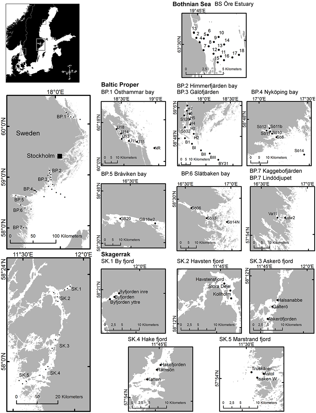
Figure 1. Map of regions and sub-areas showing sampling locations. Maps © Lantmäteriet, Gävle 2010, and permission I2014/00691.

TABLE 1

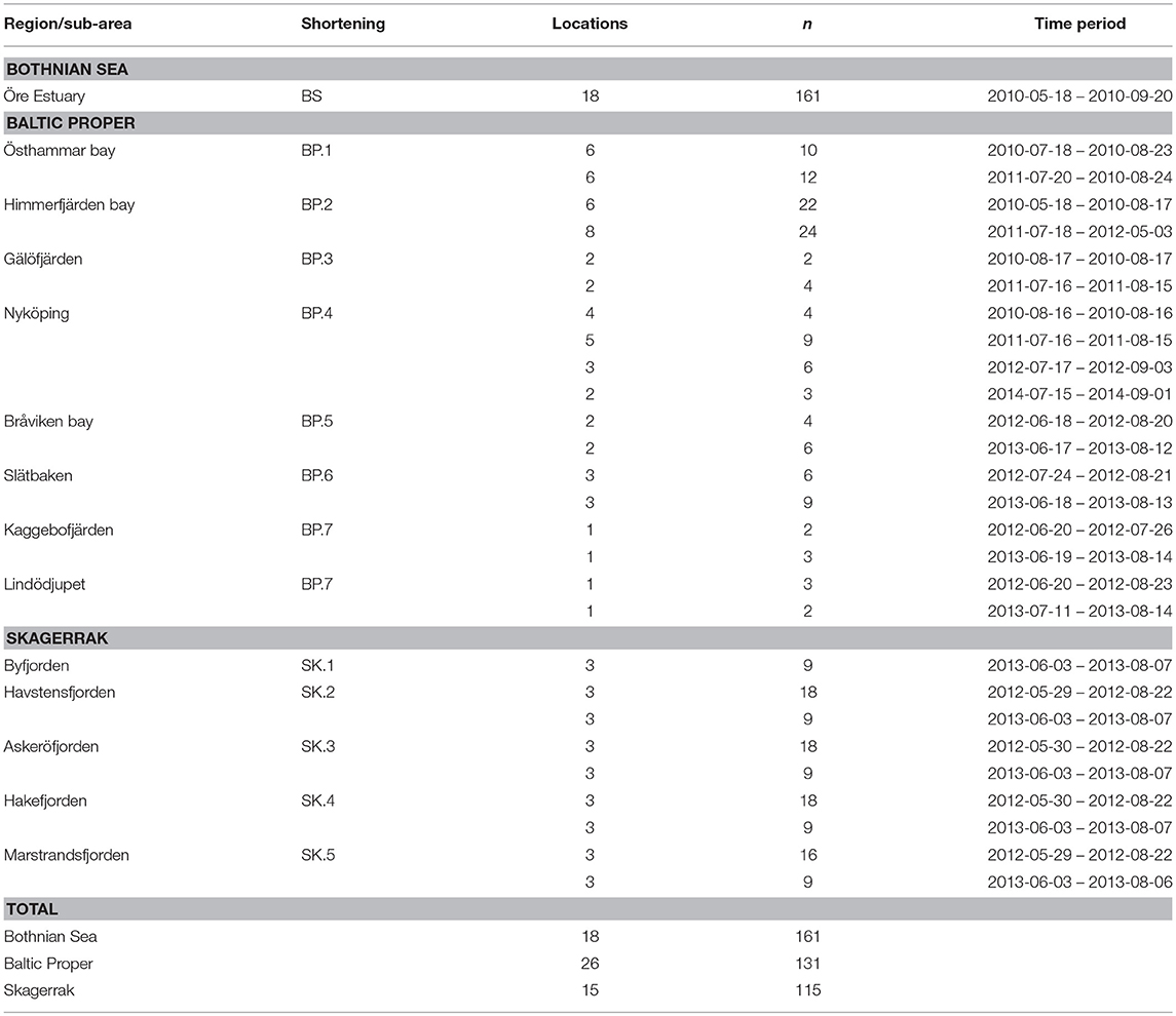
Table 1. Locations (sampling stations), number of observations (n), and measurement periods for regions and sub-areas.

Data from the BP are from seven gradients reaching inner coastal waters to the open sea (Figure 1). A total of 28 locations were sampled from June to early September 2010 to 2014 (Table 1). The Östhammar gradient (sub-area BP.1) is situated in the archipelago of Uppsala County, north of Stockholm, in southern BS but in proximity to the BP and was still included in the BP data set due to the low freshwater inflow compared to the northern part of the BS. There is only a weak salinity gradient in the BP.1 subarea, and it is the receiver of a Waste Water Treatment Plant (WWTP). The inner coastal area is eutrophicated with relatively high Chl-a concentrations. Himmerfjärden bay (BP.2), situated in the southern Stockholm archipelago, is a large fjord-like bay consisting of several basins with low freshwater input and restricted water exchange. The inner Himmerfjärden bay is a receiver of a regional large WWTP and the area shows symptoms of eutrophication, with increased phytoplankton biomass and decreased Z_SD (Engqvist, 1996; Savage et al., 2002). Gälöfjärden (BP.3) is a small, shallow bay southwest of Himmerfjärden bay with relatively high resuspension of sediments. Nyköping bay (BP.4), situated further south of Stockholm and Himmerfjärden bay, is a shallow estuary that receives the freshwater inputs of three rivers (Figure 1). The city of Nyköping and its WWTP are located in the inner part of the estuary. The large fresh water inflow and the restricted water exchange in this shallow area, create strong gradients in salinity, nutrients, Chl-a concentration and Z_SD. Bråviken bay (BP.5) is deep (ca 30 m) in its central and outer parts, but its inner-most part is rather shallow, with a high freshwater inflow from the river Motala Ström, entering through the city of Norrköping. Slätbaken (BP.6) is a relatively deep bay with sills restricting the water exchange and with a nutrient-rich freshwater inflow that seems to cause the relatively high Chl-a levels. Two locations situated south of Slätbaken, close to one-another, were also included in the study [Kaggebofjärden and Lindödjupet (sub-area BP.7)].

In the SK region, 15 locations were sampled in June to August 2012 to 2013 in an elongated fjord system between the islands Orust and Tjörn and the mainland (Figure 1, Table 1). The innermost sub-area Byfjorden (SK.1) is situated at the head of the fjord system with a large freshwater input from the river Bäveån. The discharge of the WWTP of the city of Uddevalla is located near the river mouth. Byfjorden is eutrophicated, with high levels of nitrogen and Chl-a and low Z_SD. Further sub-areas are Havstensfjorden (SK.2), Askeröfjorden (SK.3), and Hakefjorden (SK.4). Hakefjorden receives freshwater from the river Göta Älv, causing (similar as in Byfjorden) a slightly lower salinity (of ~18) than in the other sub-areas (salinities ~20). Marstrandsfjorden (SK.5) is directly connected to the open sea and has the lowest Chl-a concentrations.

In situ Data of Secchi Depth, Chl-a, CDOM, and SPM

At each sampling station all optical water quality parameters (Z_SD, Chl-a, CDOM, SPM) were measured or sampled. The water transparency (i.e., Z_SD) was measured with a white Secchi disc (25 cm in BS and most BP areas and 30 cm in diameter in SK and for some occasions in BP.2), taken on the shady side of the ship in order to avoid the influence of sun reflection on the viewer's perception of the Z_SD. A water telescope was used in the BP for Z_SD measurements in order to reduce the sun glint (Werdell, 2010; HELCOM, 2017). Water samples for measuring Chl-a, CDOM, and SPM were collected just below the surface with a special sampling bucket or a Ruttner sampler. The laboratory analyses were carried out according to established protocols or ISO- standards; Chl-a in BS and SK by HELCOM (2017) and in the BP according to Jeffrey and Vesk (1997) or HELCOM (2017), CDOM by Kirk (2011). In SK and BS samples were extracted with ethanol followed by fluorometry, in the BP extracted with ethanol or acetone followed by spectrophotometry. The analyses were conducted by both accredited monitoring labs (Jeffrey and Vesk, 1997; Werdell, 2010) as well as by a specialized bio-optics research group following established ESA MERIS protocol. The slight differences in the methods were shown to have little influence on the results, and extensive tests by the Marine Ecology Laboratory at Stockholm University prior changes from acetone to ethanol in the Chl-a extraction in various monitoring programmes, showed no difference between these methods. Also, a recent evaluation of the CDOM filtration method using glass vs. plastic filtration gear did not show any significant differences. SPM (inorganic fraction, SPIM and organic fraction, SPOM) was determined gravimetrically (Strickland and Parsons, 1972) with one replicate in the BS and the SK, three replicates per station in most cases in the BP. A more detailed description of the methods for the optical data and data collection for this study can be found in Kratzer et al. (2003), Kratzer and Tett (2009), Harvey et al. (2015a,b), and Kari et al. (2017). In Aas et al. (2014) a detailed evaluation of error sources for Z_SD measurements are given. It was found that wind-wave effects caused most errors by stirring the surface and increasing the sun glint. The use of a water telescope increased the Z_SD with 10–20% (Aas et al., 2014), whilst the wind effect at the surface caused a decrease in the same order (11%) (Sandén and Håkansson, 1996). The difference of using a disc with 10 rather than 30 cm in diameter reduced the average Z_SD by 10–20% (Aas et al., 2014). However, a recent inter-comparison between Umeå and Stockholm Universities found no significant difference when comparing the use of Secchi disks of 25 vs. 30 cm diameter. Also, the data from different regions were here analyzed separately so the results are comparable within each respective region. For this study the overall relative error for Z_SD was calculated from the coefficient of variation to below 2.6%. The error for the trichromatic Chl-a analysis is within 7–10% (Kratzer, 2000; Sørensen et al., 2007), and the SPM method has an error of about 10–13% (Kratzer, 2000; Kari et al., 2017), dependent on the range of SPM values. The error for CDOM absorption is within 6% (Harvey et al., 2015a).

Data is provided via Stockholm University, Umeå University, and SMHI upon request. Most of the Chl-a data are available within the national monitoring programme and accessible via the Swedish Oceanographic Data Center at SMHI (the SHARK-database, http://sharkweb.smhi.se), other are hosted by Umeå University or the Marine Ecology Laboratory at the Department of Ecology, Environment and Plant Sciences, Stockholm University. For the CDOM and SPM data some are also available in SHARK. The ranges of values of optical properties for all regions are shown in tables, and these ranges are required for constraining e.g., regional radiative transfer models.

Data Analysis

Correlations between Z_SD and the predicting variables, i.e., CDOM, SPM (inorganic fraction, SPIM) and Chl-a, as well as between the different predictors were tested for possible collinearity for each region. The correlations were derived applying Pearson's correlation on ln-transformed data (where ln stands for natural logarithm).

Multiple general linear models (GLMs) for Z_SD with Gaussian distribution family were used for the first data analysis step, treating “region,” “season,” and “sub-area” as categorical variables to estimate the slopes of possible spatial differences. Generally, only small amounts of SPIM originate from phytoplankton and thus, inorganic SPM (SPIM) is used here as a proxy for land-derived and/or resuspended SPM. Organic SPM is assumed to be strongly linked to phytoplankton biomass and therefore already represented by Chl-a. Hence, in the model Z_SD was response variable, and Chl-a, SPIM, and CDOM potential explanatory variables. In order to evaluate the performance of the models the modeled Z_SD was evaluated against the measured Z_SD, the Root Mean Square Error (RMSE; unit in meters), the Normalized Root Mean Square Error (NRMSE, unit in percentage) and the Mean Normalized Bias (MNB; unit in percentage) as well as 95% Confidence Intervals (CI) for the model coefficients. It should be noted that the error metrics for the models here only refer to the fit of each model to the existing regional data sets, but do not indicate how reproducible each model is. For this, an independent data set would be needed for regional model evaluation.

The second step was to apply commonality analysis based on the GLMs to reveal how much each predicting variable uniquely affects the variation in Z_SD as well as the common contribution with the other variables (i.e., that cannot be separated due to collinearity) (Kraha et al., 2012; Dormann et al., 2013; Ray-Mukherjee et al., 2014). Commonality analysis is not widely used within ecological research, but is well-established within psychology, social sciences and education. A good description with ecological examples are given in Ray-Mukherjee et al. (2014) and the use of commonality analysis splits the adjusted coefficient of determination (${\text{R}}_{\text{adj}}^2$) into a unique and a common variance of the predicting variables (Chl-a, CDOM and SPIM) to the Z_SD and thereby contributes to an improved understanding and interpretation of the different effects on Z_SD. The analysis takes the often-neglected collinearity between the predicting variables into account and enables for follow-up analyses of the GLMs.

The GLMs were used to predict the potential increases in summer Z_SD at decreased Chl-a levels, i.e., simulating an improved eutrophication status according to EU WFD and MSFD (for some outer locations). For each water body or region, the GLMs were used to calculate Z_SD using Chl-a concentrations adjusted to the respective reference (pristine) and G/M boundary Chl-a values. The reference and G/M thresholds values for Chl-a were calculated according to the specified salinity-dependent equations or the defined thresholds were used according to the Swedish Agency for Marine and Water Management (SwAM, 2012, 2015). The modeled changes in Z_SD were recalculated to deviation in % difference from the Z_SD G/M threshold for each water body or region. A deviation of 0% equals the G/M Z_SD threshold, a negative deviation indicates a lower Z_SD, and that the Z_SD threshold for G/M status has not been reached. A positive value indicates that the Z_SD threshold has been exceeded, i.e., the Z_SD is greater than the respective threshold value, thus indicating good water quality. The deviations from the G/M Z_SD threshold were then compared to the observed Z_SD for each sub-area within each region.

Assumptions of independence, normality and heteroscedasticity were tested, and all data were ln-transformed to achieve normal distribution. Residual analysis and model evaluations were performed for all statistical tests. The number of observations (n) is given for each analysis and the confidence level was set to 5%. For all graphs, statistical and data analyses R 3.0.1 was used (R Core Team, 2013).

Results

The highest average Z_SD was found in the SK area (6.2 ± 1.7 m, mean ± one standard deviation), the lowest in the BS (3.7 ± 0.9 m), and slightly higher in the BP (3.8 ± 2.3 m). Table 2 shows the ranges, means, medians, standard deviations (Stdev) and standard errors of the mean (SEM) for Z_SD, Chl-a, CDOM and SPM (total SPM, and SPIM and SPOM fractions) for the three regions. The same data are presented as boxplots for all sub-areas in the Figures S1–S3.

TABLE 2

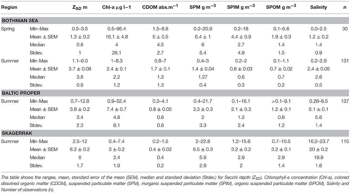
Table 2. Sampled water quality variables for the three regions with spring (May) and summer (June–August) data for the Bothnian Sea (BS) and summer (June–August) data from both the Baltic Proper (BP) and the Skagerrak (SK) regions.

Data Selection and Empirical Models

A pooled GLM for Z_SD for all regions had high predictive power (${\text{R}}_{\text{adj}}^2$ = 0.85, n = 406). However, this model was not representative for each individual region since stepwise GLMs showed significantly different model parameters between regions (Table 3). Further analyses per region showed differences between seasons and between gradients. Hence, the selected models for further analyses were focused on the summer data, the assessment period for both Chl-a and Z_SD. The BS model had moderately variable input data, except for Z_SD (Figures S1–S3), giving a relatively low predictive power (${\text{R}}_{adj}^2$ = 0.54, n = 131) for Z_SD. The SPIM component was not significant but was still included in the analysis (see motivation below). In the BP region the model chosen was based on data from all gradients (${\text{R}}_{adj}^2$ = 0.84, n = 85) except for Himmerfjärden (BP.2), as it differed significantly from the other areas (Table 3). The SK data were from five basins (sub-areas) along a gradient in a fjord system (Figure 1, Table 1) and the GLMs resulted in two models based on differences between sub-areas (Table 3). A common model for SK1, 2 and 5 (Model_S1) predicted the Z_SD fairly well with a ${\text{R}}_{adj}^2$ = 0.64 (n = 61), although the SPIM component was not significant. A common model for SK.3 and 4 (Model_S2) had a slightly lower R²adj = 0.53 (n = 54) but a significant SPIM parameter. Model_S1 was chosen for comparisons between regions since it had higher predicting power (i.e., $R_{adj}^2$) and included three out of the five sub-areas. The main models from each region (Table 3), were used for further detailed analysis and comparisons, and are from here on referred to in the text, if not stated differently. Since SPIM has strong scattering properties (Kratzer and Tett, 2009; Kirk, 2011; Kratzer and Moore, 2018), and there was a strong correlation between Z_SD and SPIM where we had the largest SPIM gradient, we chose to include the non-significant SPIM parameters (Tables 3, 4). All models had similar intercepts but different parameter coefficients.

TABLE 3

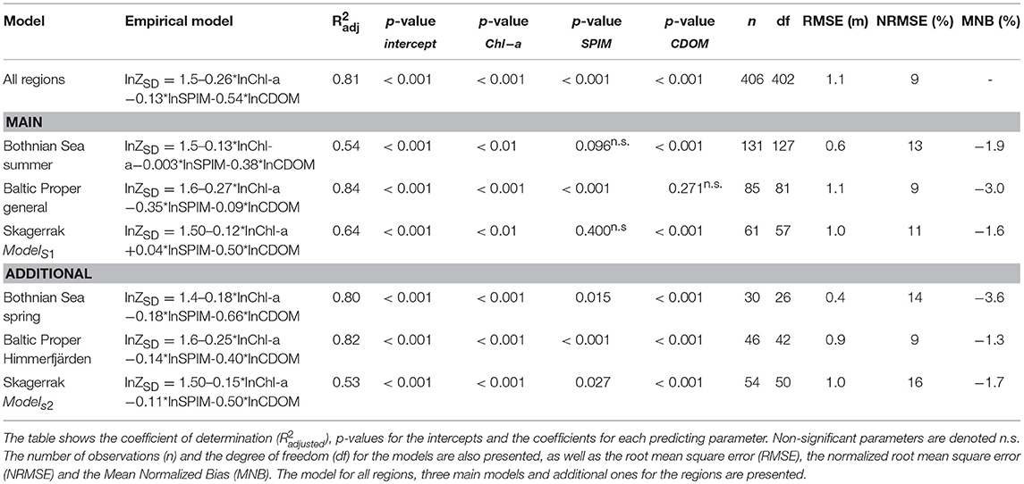
Table 3. Results from the empirical multiple regression models per region, based on the data selection from the GLM's.

TABLE 4

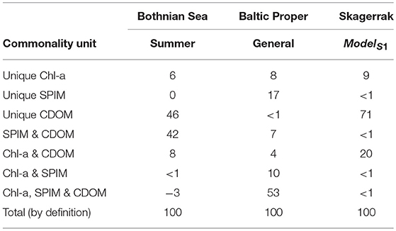
Table 4. Results of the commonality analysis, showing the percentage of contribution to the explained variations to the ${\text{R}}_{\text{adj}}^2$ for the main Z_SD models in the three regions.

Commonality Analysis

Commonality analysis showed that contribution of the various optical components to the explained Z_SD variation (${\text{R}}_{\text{adj}}^2$) was different amongst regions (Table 4, Figure 2). In the BS a large proportion was explained by CDOM alone (46%), together with the paired interaction of CDOM and SPIM (42%). The SPIM component had no unique effect and Chl-a alone explained only 6%, whilst CDOM and Chl-a combined contributed somewhat more (8%) to the variations in Z_SD. The common interaction effect of all three variables in the BS was very low and even negative. In contrast, the common interaction effect of all three variables (~53%) together with the interaction of Chl-a and SPIM (~11%) explained most of the variation in Z_SD in the BP. In the SK, CDOM alone explained more than two thirds (~70%) of the variation in Z_SD. SPIM contributed uniquely with < 1% and the shared, interactive commonalities were negative, but very close to zero. Moreover, Chl-a had the most pronounced unique effect on Z_SD in the SK (9%).

FIGURE 2

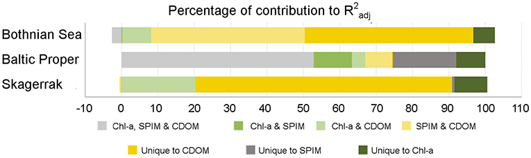
Figure 2. Bar chart of the commonality analyses based on the main empirical GLMs (see Table 3). The separated commonalities are presented as % of the contribution to the ${\text{R}}_{\text{adj}}^2$ for each model.

Correlation and Multiple Regression Analysis

Correlation analysis among the predicting variables and Z_SD for each region (Figure 3, Table 5) were used to evaluate the GLMs and the commonality analyses, and to visualize the data. Z_SD was inversely correlated to Chl-a in all regions, with the strongest correlation in the BP, moderate in the SK and the weakest in the BS (Figures 3A,D,G, Table 5). The relationship between Z_SD and CDOM was strong and inverse in all regions (Figures 3B,E,H, Table 5). The correlation between Z_SD and SPIM was inverse and strong in the BP, but weaker in the BS and absent for SK (Figures 3C,F,I, Table 5). Correlations between the predicting variables (i.e., the optical components) also differed among the regions (Figure 4, Table 5). There were strong positive correlations between Chl-a and CDOM and between Chl-a and SPIM in the BP, but these were absent or weak in the BS and the SK (Figures 4A,B,D,E,G,H, Table 5). The relationship between CDOM and SPIM was on the other hand positive and significant in the BS and the BP but not in the SK (Figures 4C,F,I, Table 5).

FIGURE 3

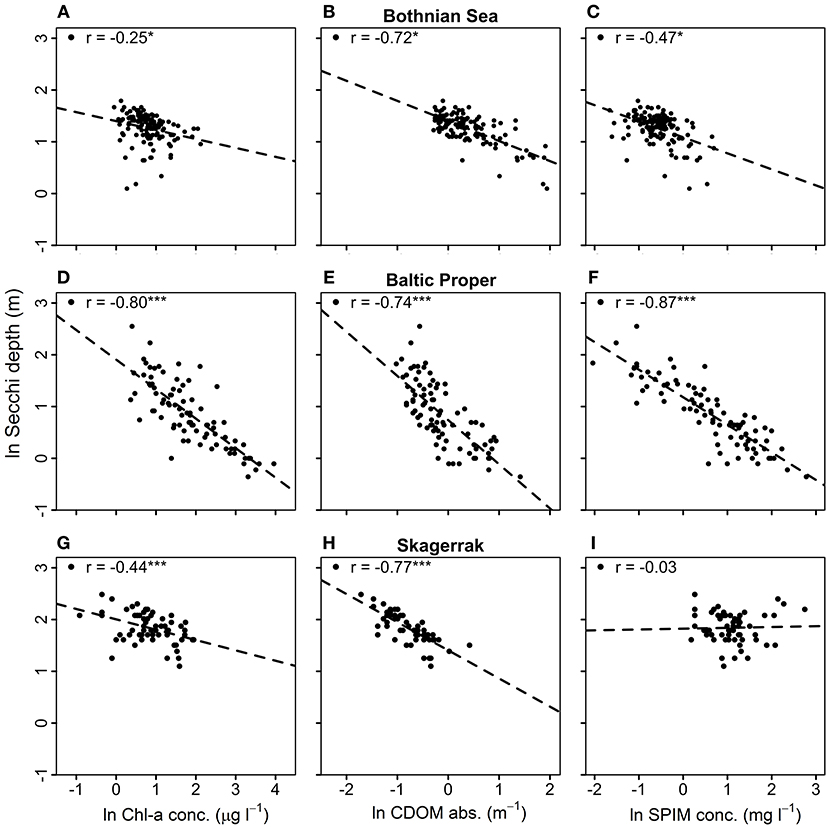
Figure 3. Correlation plots between Secchi depth, Z_SD (m) and the predicting parameters; Chl-a [μg l⁻¹] (left), CDOM (m⁻¹) (middle), and SPIM [g m⁻³] (right). Graphs (A–C) show data from the Bothnian Sea (BS), (D–F) from the Baltic Proper (BP) and (G–I) from the Skagerrak (SK). The Pearson correlation coefficient, r, is shown for each data-set, where *, *** denotes significant correlations at 0.01 and 0.0001 levels and no star indicates non-significance. All data have been natural log-transformed.

TABLE 5

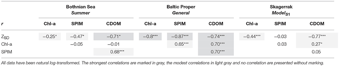
Table 5. Table showing the Pearson correlation coefficient, r, for each data set, where *, *** denotes significant correlations at 0.01 and 0.0001 levels and no star indicates n.s.

FIGURE 4

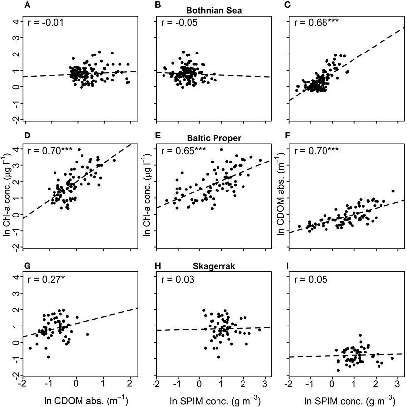
Figure 4. Correlation plots between Chl-a [μg l⁻¹] and CDOM (m⁻¹) (left), Chl-a and SPIM [g m⁻³] (middle) and CDOM and SPIM (right). Graphs (A–C) show data from the Bothnian Sea (BS), (D–F) from the Baltic Proper (BP), and (G–I) from the Skagerrak (SK). The Pearson correlation coefficient, r, is shown for each data-set, where *, *** denotes significant correlations at 0.01 and 0.0001 levels and no star indicates non-significance. All data are natural log-transformed.

Model Performances in Baltic Sea Regions

The main models predicted Z_SD well with ${\text{R}}_{\text{adj}}^2$ between 0.54 and 0.84 and with a rather high precision (RMSE 0.6–1.1 m, equivalent to a NRMSE of only 9–13%) and a very high accuracy with a low bias (MNB only 1.6–3%) (Table 3). The relative errors (RMSE) in this study were in the same range as e.g., found in the Oslo fjord in the Skagerrak (Aas et al., 2014). Outliers have a large influence on the error statistics (Figure 5 and Figure S4). In the BS model some Z_SD observations deviated from the model predictions both in the lower, <1.5 m and higher, >5 m Z_SD range (Figures 5A,B). This explains the lower ${\text{R}}_{\text{adj}}^2$ and the NRMSE of 13% of this model. The BP model performed better over the full range of Z_SD, except for a few very high values (Figures 5C,D). Similarly, the SK model captured the full range of Z_SD well, also for the highest values with a slightly higher dispersion in the lower Z_SD range (Figures 5E,F). The graphs for the additional models are presented in the Figure S4, as all models were used for the respective sub-areas in the analysis of Chl-a influence on EU Directive Z_SD targets. Overall, the biases for all models were low (slightly negative), indicating a high precision of the estimated Z_SD from the models, with an insignificant underestimation of the predicted Z_SD, as all MNB were <4% (Table 3). The Confidence Intervals (CI) of the model intercepts and coefficients were calculated using a two-sided 95% CI and are presented in Figure 6 and Table 6. The Chl-a coefficients showed the smallest difference among regions and the narrowest CI, indicating a high precision of the estimated coefficients. The SPIM coefficients also had a relatively small range of CI while the range was larger for the CDOM coefficients. The intercepts were all very close to each other, with smaller CI for the main models. Generally, the coefficients and intercepts for SK and BS were closer to each other than to those for BP.

FIGURE 5

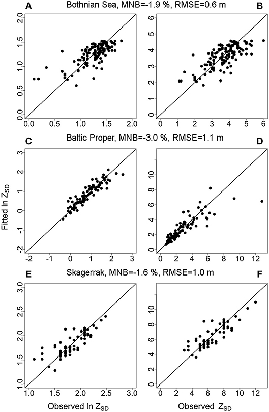
Figure 5. Graphs showing the observed Secchi depth, Z_SD (m) on the x-axis vs. fitted Secchi depth, Z_SD on the y-axis for the main models per region. The left panel (A,C,E) shows the values in natural log scale and the right panel (B,D,F) in back-transformed normal scale. The Mean Normalized Bias; MNB and Root Mean Square Errors; RMSE are indicated for each model. Graphs for the additional models are shown in the Figure S4.

FIGURE 6

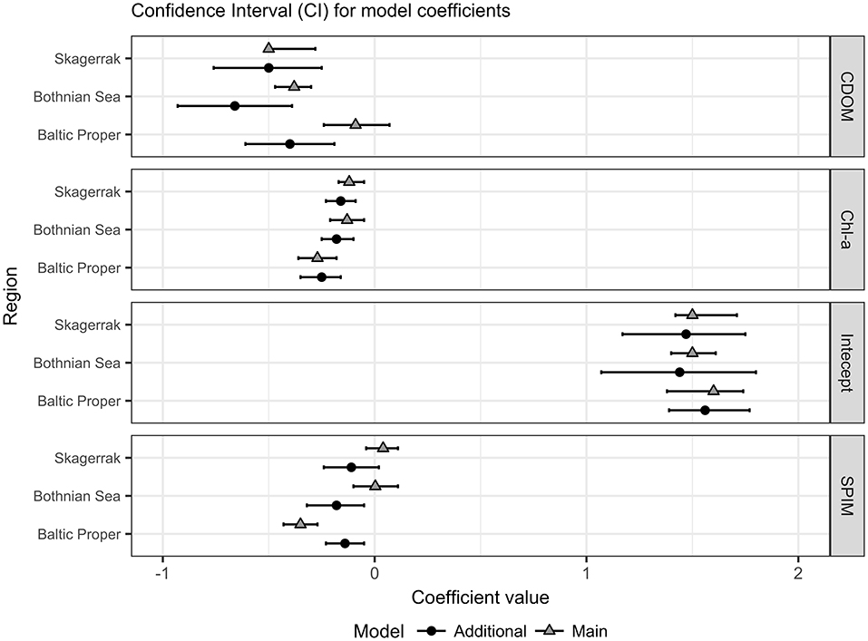
Figure 6. Confidence Interval (CI) for the model coefficients in natural log scale (see Table 3 for model presentations); CDOM slopes, SPIM slopes, Chl-a slopes and Intercepts for each region (BS; BP and SK). Triangles indicate the main models and filled circles the additional. The bar lines show the 95% CI of each estimated coefficient.

TABLE 6

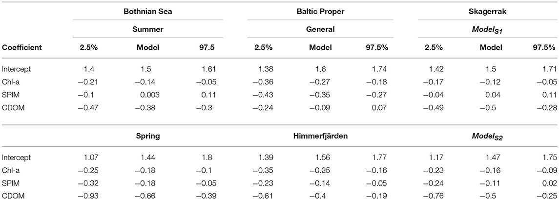
Table 6. Table showing the 95 % Confidence Interval (CI) of the intercepts and coefficients for the models.

Chl-a Influence on the EU Directive Secchi Depth Targets

For each sub-area within the regions, the deviations from the G/M Z_SD threshold were calculated for observed and for modeled Z_SD-values (by the derived empirical GMLs). The modeled changes in Z_SD were obtained by adjusting the Chl-a levels in the models to (1) G/M value of Chl-a and (2) to the Chl-a reference value (Figure 7). In the BP all observed Z_SD values were below the G/M Z_SD threshold, except one off-shore station in BP.1. All modeled Z_SD values increased but only a few reached or exceeded the Z_SD threshold for good environmental status. Even though the Chl-a concentrations were lowered considerably (compared to the observed values), many of the modeled Z_SD values in the sub-areas were still more than 50% below the Z_SD threshold. In the SK the measured Z_SD were generally above or near the G/M Z_SD threshold, indicating good environmental status for Z_SD. For simulated reference Chl-a concentrations there was some increase of Z_SD for the sub-areas SK.3 & 4 (model_S2), with very few observations below the threshold (Figure 7). However, for the sub-areas SK.1–2 & 5 (model_S1), the modeled Z_SD for reference and G/M Chl-a decreased to near or even below the Z_SD threshold (Figure 7). This is explained by the low observed Chl-a values, many already below the Chl-a G/M threshold, and that the G/M Chl-a values used in the models were higher. In the BS most of the observed Z_SD values were above the G/M Z_SD threshold and the distance increased even more for the Z_SD modeled from reference Chl-a values (Figure 7). The median of the modeled Z_SD values with the G/M threshold for Chl-a was not improved.

FIGURE 7

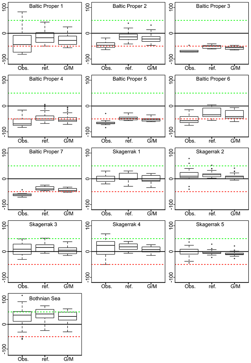
Figure 7. Boxplots of the % differences to the Good/Moderate (G/M) thresholds of Secchi depth, Z_SD for the respective water bodies within the WFD or the MSFD. The solid line denotes the G/M level for Z_SD; the upper dashed green line 50% above; and the lower dashed red line 50% below the Z_SD threshold. The boxes for the different sub-areas represent observed Z_SD (Obs), modeled Z_SD with Chl-a concentrations set to the respective reference value (ref) and with Chl-a concentration set to the G/M value for Chl-a. The horizontal lines in the boxplots are the median values, horizontal edges the 25th and 75th percentiles, the whiskers indicate the min and max observations within 10th and 90th percentiles, and open circles represent outliers.

Discussion

Empirical models were built to estimate the Z_SD, based on the optical components Chl-a, CDOM and SPIM. The results show that in the studied regions the components contribute differently to the variations in the Z_SD. Our results demonstrate that contributions from all optical variables to the variation in Z_SD affect the possibility of reaching the current G/M threshold of Z_SD as defined by the WFD and the MSFD.

Different Empirical Models Indicate Different Optical Conditions

The empirical models and commonality analyses reveal a variability and inconsistency in the collinearity between the predicting variables among the studied coastal regions, indicating complex optical conditions caused by different proportions of the three optical components. For example, a large difference in the proportion of inorganic matter, which is strongly scattering, to organic matter, which is highly absorbing, will have a great effect on K_d as it is a non-linear function of both absorption and scatter (Kirk, 2011) (Equation 1). In the BS the SPIM coefficient in the main model was not significant but the commonality analysis showed that together with CDOM, SPIM still had a strong collinear influence on the variation in Z_SD. A strong unique effect was seen for CDOM (~46%). Riverine CDOM loads are generally much higher in the BS than in the BP (Harvey et al., 2015a) and the SK (Figure S2). In the BS gradient there were very high median values of CDOM, even during the summer (1.7 m⁻¹) but the SPIM was relatively low (0.6 g m⁻³) (Table 2). The high background CDOM absorption leads to a relatively low reflectance and makes the water appear rather dark. Thus, a comparatively small increase in SPIM scattering will have a relatively large influence on the reflectance and, thus on the Z_SD. The commonality analysis showed a rather interesting result for the SK, here the variation in the Z_SD was even more driven by CDOM alone (70%) than in the BS (Figure 2, Table 4) even though the levels of CDOM were much lower (0.4 on average), and the SPIM values relatively high (about 3.2 g m⁻³ on average), which indicates that overall, the light attenuation should be dominated by SPIM scatter (Equation 1). However, the total effect of SPIM (unique and common effects) on Z_SD variation was much less in the main model for SK (< 1%) than in the and BP, where SPIM contributed 40 and 85%, respectively. There is an important distinction between which optical component that dominates the light attenuation—e.g., scattering from SPIM in the SK—and which component that drives the variability in light attenuation. The commonality analysis explains the contribution of the optical components to the variability of Z_SD and is completely dependent on the covariation and concentrations of the optical components. The difference between regions may partly be due to the effect of tidal action at the west coast, which is hardly detectable in the other two regions. The tidal range on the Swedish SK coast is rather low, ca. 30 cm, compared to many other seas, but higher than in the Baltic Sea, where it is only in the range of a few centimeters. Tidal action may explain a relatively high background of SPIM in the SK and influence the CDOM gradient. During high tides, open sea waters currents move into the fjords at the west coast, markedly decreasing CDOM concentrations (unpublished data from Gullmars fjord, measured by S. Kratzer), whereas during low tides the water runs in the reverse direction, i.e., from the inner fjords to the outer sea, which markedly increases the CDOM concentrations. The results of the commonality analysis can to a large extent be explained by the collinearity between different parameters in the regions, as reflected in the correlation analysis. For example, the correlation between Z_SD and SPIM was low for the main SK model, as reflected in the low SPIM coefficient in the model. A weak correlation (r = 0.27) was found between the Chl-a and CDOM, which was also reflected in the shared commonality between the two parameters.

Another explanation for low influence of SPIM is that the commonality analysis is based on multiple regressions (assuming a linear relationship between the parameters) and is thus dependent on the model's accuracy to predict Z_SD. The coefficients of determination for the models were moderate both for the SK (R² = 0.64) and the BS (R² = 0.54) and the commonality analyses only explain ~50–65% of the variation in Z_SD. It should therefore not be used as a tool to explain the (optical) physics behind Z_SD variability but is valuable for a rough estimation on which parameters may drive the variability. Figures 3, 4, however, show that in the BP there are very strong correlations between Z_SD and all three main optical components. The results of the commonality analysis also showed that SPIM in BP was here the largest single contributor to Z_SD variability (Table 4). The largest effect on the variation in the BP, however, was from the shared commonality of all three components (~53%), which was clearly seen in their strong negative correlation with Z_SD (Figure 3) and the strong positive correlation (indicating strong collinearity) among them (Figure 4). This differed from the other regions that had very low values for the three fold-shared commonalities. The largest total effect of Chl-a (~75%) was found in the BP region, even though the unique effect was slightly stronger in the SK region. However, in the SK there was also a substantial effect shared with CDOM (20%). When evaluating the results of commonality analysis, it is important to stress that the analysis describes the unique separate and combined statistical effects of each variable to the explained variation in the ${\text{R}}_{\text{adj}}^2$. Consequently, the same percentage value for a unique contributor in a certain region can here mean different actual contribution to the variation in Z_SD (Ray-Mukherjee et al., 2014). For example, will the 1 % CDOM contribution from the commonality model in BP correspond to a CDOM contribution of 8.4% of ${\text{R}}_{\text{adj}}^2$ variation CDOM, whereas the 1 % SPIM contribution in the SK model corresponds to 6.4% explanation of ${\text{R}}_{\text{adj}}^2$.

In summary, based on the commonality analyses the variations in Z_SD were overall mostly governed by CDOM, both uniquely and together with SPIM in the BS, by all three parameters jointly and uniquely by SPIM in the BP, and by CDOM, uniquely and together with Chl-a, in the SK. The relative contribution of the inherent optical components to K_d for a large lake dataset from Norway and Sweden was evaluated in Thrane et al. (2014), where also CDOM was found to be the dominant component, followed by Chl-a and non-algal particles, water excluded. Kratzer and Tett (2009) found that K_d490 was predominantly determined by CDOM absorption, both in the open and coastal Baltic Sea. In coastal areas the effect of SPM scatter also had a strong optical influence (decreasing with distance to the shore), while Chl-a had a relatively small optical influence, both in the open sea and coastal areas.

Factors Influencing the Optical Variables

Some of the differences among regions seen in the commonality analyses models may be explained by the differences in the inherent optical properties among CDOM, SPIM, and Chl-a jointly influencing the under-water light conditions and modulated by changes in physical and hydrological schemes. The strong correlations observed between CDOM and SPIM are most likely caused by a strong influence of terrestrial run-off, leading to a large variation in both CDOM and SPIM, even though run-off is lower in summer than in spring. However, the same pattern was not seen in SK, where there on the other hand is a pronounced tidal effect. Dupont and Aksnes (2013) showed that also the distance from shore and the bottom depth are significant factors affecting Z_SD, both in the Baltic Sea and the North Sea. In Danish waters, suspended material and Chl-a was found to be negatively correlated to Z_SD, with a pronounced effect on the variation in Z_SD (Nielsen et al., 2002) similar to our results. Resuspension or erosion of sediments (i.e., increase of SPIM) have been shown to affect water optics in other seas as shown by Otto (1966), Devlin et al. (2008), and Capuzzo et al. (2015), as well as for the BP (Kratzer and Tett, 2009) and thus may also be pronounced in many BS coastal areas less dominated by freshwater run-off than in this study. Even though the SPIM was relatively high in the SK and seemed influenced by tidal dynamics that may lead to a relatively strong resuspension of inorganic sediments it showed an unexpectedly small effect on Z_SD variation.

Nutrient input has also been found to be negatively correlated to the Z_SD, by increasing Chl-a levels (Nielsen et al., 2002; Fleming-Lehtinen and Laamanen, 2012; Aas et al., 2014). Nutrient inputs are often increased by high run-off that also introduces more allochthonous CDOM and SPM into the ecosystem, as is reflected in the correlations between these variables in this study and in coastal gradients by Kratzer and Tett (2009) and Capuzzo et al. (2015). Phytoplankton can be a substantial fraction of total SPM, which means that Chl-a are often positively correlated with SPOM (e.g., Nielsen et al., 2002). But Chl-a may also correlate with SPIM, e.g., due to the silica in diatom blooms or through run-off, increasing both SPM and nutrients that increase Chl-a. Assuming a phytoplankton carbon to Chl-a ratio of 40 (Sathyendranath et al., 2009), a carbon content of 40% and (a high) ash content of 20% (~25–40% in diatoms) of dry weight (Whyte, 1987), the range of Chl-a from 1 to 52 μg/l (median 5 μg/l) in the BP should correspond to SPIM concentrations of 0.02 to 1 mg/l (median 0.1), about a magnitude lower than the observed range of SPIM (0.1 to 16 mg/l, median 2.1). The SPIM found in algal detritus should also contribute, possibly in the same concentration range. This means that, overall the cellular contents of inorganics is relatively small in algal cells compared to terrestrial inorganic matter originating from freshwater or coastal erosion.

Kratzer and Moore (2018) investigated the scattering and absorption properties of the Baltic Sea in comparison to other seas and oceans. They found that besides an optical dominance of CDOM absorption, there was also a clear indication of different optical water types—open sea vs. coastal waters. Thus, in optical models different parameterization may have to be sought for these different water types. This should also be considered when investigating the effect of all three main optical components on Z_SD. Inner coastal waters are often dominated by SPIM scattering (Kratzer and Tett, 2009; Kari et al., 2018), which will also clearly affect the Z_SD. Open sea waters are more dominated by CDOM absorption- and during times of phytoplankton blooms also by phytoplankton absorption and scatter. The proportion of inorganic to total SPM decreases when moving from inner coastal to more open sea waters (Kratzer and Tett, 2009; Kari et al., 2018). It is therefore recommendable that current monitoring programs also include measurements of SPIM in the coastal zone. In the open sea, total SPM or turbidity measurements can be used to indicate phytoplankton or cyanobacteria blooms, as the organic fraction usually falls out very close to the coast (Kratzer and Tett, 2009; Kari et al., 2018). In all regions CDOM correlated quite strongly with Z_SD (r ranging between −0.71 and −0.77) (Table 5), which makes CDOM a very important optical variable to measure in all areas.

Climatological models for the Baltic Sea predict more land run-off due to an increase in precipitation, especially in the northern Scandinavian regions (Meier et al., 2012a,b). This might lead to a brownification due to an increase in humic matter and suspended organic material to the sea (Larsen et al., 2011; Meier et al., 2012a). Although the relationships between K_d and Z_SD are variable in the Baltic Sea, stronger light absorption due to climate change would affect the light climate and the conditions for primary production by an increase in K_d and thus a decrease in Z_SD (Kowalczuk et al., 2005; Kratzer and Tett, 2009; Harvey et al., 2015a). Hence, the predicted brownification due to an increase in precipitation in northern Scandinavia may have a dominant effect over a possible decrease in Chl-a concentrations due to recent and future reductions in nutrient loads by effective management programs, maybe resulting in unchanged Z_SD.

Secchi Depth and Implications for Eutrophication Management

Our results show that using Z_SD as a direct eutrophication indicator may be misleading, as the empirical models, the commonality analyses and the correlations all show that Z_SD is more strongly related to CDOM and SPIM than to Chl-a, or that these variables are inter-correlated in the coastal gradients. Hence, the common assumption that a strong direct inverse relationship with Chl-a makes Z_SD a suitable water quality indicator has important limitations in the Baltic Sea. Some anthropogenic measures to reduce nutrient load from run-off, e.g., changes in land use or wetland area, are also likely to affect the input of CDOM and SPM to coastal waters and might mitigate climate change effects. However, natural gradients of CDOM and SPM from the coast to the open sea (Kratzer and Tett, 2009; Harvey et al., 2015a) will likely have a main influence on the response of the Z_SD to anthropogenic changes. Even more important is that those relationships vary with region, sub-areas and season, meaning that the same Z_SD value may indicate quite different environmental and optical conditions, influencing the management efforts needed for certain Z_SD improvements. In different optical water types (e.g., clear ocean vs. coastal waters) the same change in Z_SD expressed in meters can imply very different ranges and combinations of the optical components (Kirk, 2011). Due to the logarithmic attenuation of light in the water, a decrease in Z_SD from 2 to 1 m is related to much larger changes in concentrations and absorption by optical components than a Z_SD decrease from 10 to 9 m (Dupont and Aksnes, 2013), implying very different management efforts and costs.

Long-term decreases in Z_SD have been observed in both the open Baltic Sea and the North Sea. In the open Baltic Sea, increased Chl-a have been linked, to some extent, to a decrease in Z_SD (Sandén and Håkansson, 1996; Fleming-Lehtinen and Laamanen, 2012; Dupont and Aksnes, 2013), but the potential importance of CDOM and SPIM was not evaluated in these studies. Z_SD is commonly used as indicator of eutrophication (HELCOM, 2007; European Commission, 2008, 2010; Karydis, 2009; Fleming-Lehtinen and Laamanen, 2012). In the WFD and the MSFD, targets and thresholds for both Z_SD and Chl-a are used to classify if water bodies meet the goals of good eutrophication status (SwAM, 2012, 2015), influencing management action plans. The long-term time-series of Z_SD in open sea areas and the Chl-a to Z_SD relationships have been used to establish reference chlorophyll values (Hansson and Håkansson, 2006; Larsson et al., 2006). Due to the lack of long-term data for coastal areas, these results have been extrapolated to the coastal zone and neighboring water bodies (Hansson and Håkansson, 2006). Because of the correlations of Chl-a with SPM and CDOM in coastal gradients the relationships may overestimate the response of Z_SD to changes in nutrients levels and chlorophyll.

When the coastal reference and G/M Chl-a levels were applied in the different coastal areas to our models, the G/M levels of Z_SD were unlikely to be met in the BP and in the SK region, but in the BS, as the latter is less eutrophicated. In the SK the observed Z_SD met or were close to the G/M levels and changing the Chl-a levels mostly had a negative effect on the Z_SD. In the BP the target levels of Z_SD were met only in a very few cases, even when adjusting the Chl-a levels to the reference conditions. The results clearly indicate that reducing Chl-a alone will not be enough to reach a good status also for Z_SD depth, or that the current Z_SD targets are not realistic. Riemann et al. (2015) showed that the modest increase in Z_SD measured in Danish coastal waters (over 25 years) was in general not only a response to reduced nutrient levels and Chl-a concentrations but was related to changes in other optical components such as lower SPM concentrations, and thus less scattering. An increase in SPIM at constant levels of total dissolved carbon (over 21 years), was found to determine the K_d in a Danish fjord, despite substantial nutrient reduction leading to a decrease in Chl-a (Carstensen et al., 2013). Therefore, it may be questioned if the G/M levels of Z_SD can be reached at all for water bodies with high concentrations of CDOM or SPIM, that are common in coastal waters. In fact, the reference and G/M thresholds for Z_SD will be overestimated in such areas. The management (as well as the monitoring programs) could preferably be changed to be adapted more to the background values of CDOM and to some extent SPM.

Another important water quality indicator is the depth distribution of submersed aquatic vegetation (Dennison et al., 1993; Middelboe and Markager, 1997), which is affected by eutrophication because of lowered water transparency (European Commission, 2000, 2010; SwAM, 2015). An appropriate estimation of Z_SD target and reference levels taking into account natural gradients in CDOM and SPIM is important for setting correct goals for the depth distribution of submersed aquatic vegetation (Dennison et al., 1993; Gallegos, 2001; Carstensen et al., 2013).

The correlation and commonality analyses showed that the main optical parameters are strongly linked in the Baltic Sea, and changes in Chl-a concentrations generally co-occur with changes in both SPIM and CDOM. Our application of the models when testing the effect on Z_SD by changing Chl-a, assumes that we can change one parameter while keeping the other parameters constant. This approach can be somewhat misleading due to the general collinearity between variables. Strictly speaking, all three main optical components tend to change in tandem along a specific gradient, and it is therefore not correct to assume that the model fully captures the response when both CDOM and SPIM values vary while Chl-a is assigned to a fixed value. However, this was done in Figure 7 for water types with defined fixed reference values and G/M-boundaries for Chl-a (BS and SK) in order to show what an effect a change in Chl-a has in different coastal waters with different optical properties and composition. For the BP, Swedish Chl-a reference values are linked to the salinity gradients so from this point of view, they are more realistic. Anyhow, a certain nutrient reduction, affecting Chl-a levels, should have different effects in water bodies with different levels of CDOM and SPIM. The effect would be largest in the SK, which has stronger unique and common effects from Chl-a concentration than found for the other areas. The other variables are more important, both uniquely and interactively, in the BS and the BP. Therefore, the effects of reduced Chl-a levels on Z_SD are not only generally lower than predicted from simple Chl-a to Z_SD relationships, they are also very difficult to estimate with a high degree of certainty in these areas.

Monitoring of eutrophication within the WFD and the MSFD does not only take Chl-a and Z_SD into account, but they are two of the most important indicators used- together with nutrients, biovolume, oxygen conditions, and phytoplankton composition. Recent assessment of the eutrophication status e.g., within HELCOM and the Holas II assessment (HELCOM, 2018) use an integrated eutrophication assessment tool, considering the joint status of all indicators. A way forward for using Z_SD as an indicator for eutrophication is to refine the Z_SD reference values and thresholds based on the natural relationship among the optical parameters, preferably by optical modeling also taking historical data into account. Usually optical data sets have not been commonly collected within monitoring programmes but K_d often is available from measured light profiles. Information about Chl-a and K_d could then be used to model the historical reference values for Z_SD.

Conclusions

Secchi depth is a water quality indicator that is easy and relatively inexpensive to measure. However, it is very hard to interpret in the complex optical conditions found in the Baltic Sea. The same Z_SD can result from very different combinations of phytoplankton, SPM and CDOM. Changes in Z_SD are commonly influenced by changes in all optical constituents in the water column, not only by changes in the Chl-a concentration. With its uniquely long historical record, Z_SD is, and will continue to be, an important general water quality indicator, as good water transparency means a lot to laypeople. Hence, as Z_SD responds not only to Chl-a and phytoplankton, it is not an appropriate indicator for eutrophication assessment in areas such as the Baltic Sea, especially in coastal areas, with gradients in CDOM and SPIM. This has implication for management of the Baltic Sea, as well as of many other coastal and eutrophic waters. When setting reference and target levels for Z_SD for use in management, it is imperative to consider also the contribution and response of the other two main optical components—CDOM and SPIM- besides Chl-a. Knowledge of local conditions and the causes and response in optical changes of a given water body is crucial for developing accurate and attainable goals in the WFD and the MSFD, both for Z_SD and for the depth distribution of benthic vegetation. Measurements of both absorption and scattering properties combined with bio-optical modeling may help to identify alternative approaches to using Z_SD as indicator for eutrophication. For example, the Chl-specific absorption of phytoplankton could be used as indicator for eutrophication as it is one of the main parameters determining the ability of phytoplankton to absorb light and thus their productivity. As the productive status of a water body may also be light limited, Z_SD may still be an important co-factor for describing the eutrophication status of a water body. For routine monitoring programs at least the measurement of SPM (or turbidity), SPIM and CDOM should be feasible. Turbidity can be used as a proxy for SPM scattering and CDOM is measured directly in terms of absorption. Absorption and scattering can also be derived from satellite remote sensing data via the Copernicus program from the European Commission launched by ESA, especially using data from the Ocean Land Color Instrument (OLCI) on Sentinel-3. Using these inherent optical properties may guide a new way forward in eutrophication assessment as the absorption of phytoplankton as well as the K_d can be derived from remote sensing data and is directly related to the productive status of the water body. These additional optical measurements both from in situ and remote sensing would provide invaluable information to interpret water quality and would improve both water quality assessment and management.

Author Contributions

ETH and SK are responsible for the original research idea, which was further developed together with JW. SK was in charge of the research in Himmerfjärden and the Baltic Proper gradients, together with JW. BK was responsible for the research in the Skagerrak region and AA for the Bothnian Sea region. Data analysis and model evaluation has been conducted by ETH together with primarily SK and JW with inputs from AA and BK. ETH is responsible for writing the article, but all co-authors have contributed significantly and participated in the discussions, especially SK and JW.

Funding

Funding was provided by the FORMAS funded initiative Strategic Marine Environmental Research programs Baltic Sea Adaptive Management (BEAM) based at Stockholm University and Ecosystem dynamics in the Baltic Sea in a Changing climate perspective (EcoChange) based at Umeå University, The Swedish National Space Board (147/12, 110/16, 175/17), and the Swedish Environmental Protection Agency and the Swedish Agency for Marine and Water Management research program Waterbody Assessment Tools for Ecological Reference conditions and status in Sweden (WATERS) [10/179 and 13/33]. Supportive funding was also provided by the Svealand Coastal Water Association (Svealands kustvattenvårdsförbund, SKVVF). The Bothnian Sea data were collected under the EcoChange program. Baltic Proper and Skagerrak data were collected in the WATERS research program. SKVVF contributed with data for areas BP.1-4.

Conflict of Interest Statement

The authors declare that the research was conducted in the absence of any commercial or financial relationships that could be construed as a potential conflict of interest.

Acknowledgments

We would like to acknowledge all colleagues who collaborated in the monitoring programs and helped collecting and analyzing water samples (i.e., the Water Quality Association for the Bohus Coast sharing data and aid with sampling, the Marine Ecology Laboratory at the Department of Ecology, Environment and Plant Sciences, Stockholm University, Umeå Marine Sciences Center, and SKVVF). Samplings in the Bothnian Sea were performed by the EcoChange Research program. Sampling in the Skagerrak was coordinated with the BOX-project. The latter was coordinated by Prof. Anders Stigebrandt at the University of Gothenburg. Special thanks to Elina Kari and Madher Adalla for excellent help with the lab analyzes. We would also like to thank Prof. Ragnar Elmgren for valuable comments at an early stage of the manuscript.

Supplementary Material

The Supplementary Material for this article can be found online at: https://www.frontiersin.org/articles/10.3389/fmars.2018.00496/full#supplementary-material

References

Aas, E., Høkedal, J., and Sørensen, K. (2014). Secchi depth in the oslofjord–skagerrak area: theory, experiments and relationships to other quantities. Ocean Sci. 10, 177–199. doi: 10.5194/os-10-177-2014

CrossRef Full Text | Google Scholar

Alikas, K., Kratzer, S., Reinart, A., Kauer, T., and Paavel, B. (2015). Robust remote sensing algorithms to derive the diffuse attenuation coefficient for lakes and coastal waters. Limnol. Oceanogr. Methods 13, 402–415. doi: 10.1002/lom3.10033

CrossRef Full Text | Google Scholar

Andersen, J. H., Carstensen, J., Conley, D. J., Dromph, K., Fleming-Lehtinen, V., Gustafsson, B. G., et al. (2017). Long-term temporal and spatial trends in eutrophication status of the Baltic Sea. Biol. Rev. 92, 135–149. doi: 10.1111/brv.12221

PubMed Abstract | CrossRef Full Text | Google Scholar

Blomqvist, S., and Larsson, U. (1994). Detrital bedrock elements as tracers of settling resuspended particulate matter in a coastal area of the Baltic Sea. Limnol. Oceanogr. 39, 880–896. doi: 10.4319/lo.1994.39.4.0880

CrossRef Full Text | Google Scholar

Boyce, D. G., Lewis, M. R., and Worm, B. (2010). Global phytoplankton decline over the past century. Nature 466, 591–596. doi: 10.1038/nature09268

PubMed Abstract | CrossRef Full Text | Google Scholar

Capuzzo, E., Stephens, D., Silva, T., Barry, J., and Forster, R. M. (2015). Decrease in water clarity of the southern and central north sea during the 20th century. Global Change Biol. 21, 2206–2214. doi: 10.1111/gcb.12854

PubMed Abstract | CrossRef Full Text | Google Scholar

Carstensen, J., Krause-Jensen, D., Markager, S., Timmermann, K., and Windolf, J. (2013). Water clarity and eelgrass responses to nitrogen reductions in the eutrophic skive fjord, denmark. Hydrobiologia 704, 293–309. doi: 10.1007/s10750-012-1266-y

CrossRef Full Text | Google Scholar

Dennison, W. C., Orth, R. J., Moore, K. A., Stevenson, J. C., Carter, J., Kollar, S., et al., (1993). Assessing water quality with submersed aquatic vegetation. BioScience 43, 86–94. doi: 10.2307/1311969

CrossRef Full Text | Google Scholar

Deutsch, B., Alling, V., Humborg, C., Korth, F., and Mörth, C. M. (2012). Tracing inputs of terrestrial high molecular weight dissolved organic matter within the Baltic Sea ecosystem. Biogeosciences 9, 4465–4475. doi: 10.5194/bg-9-4465-2012

CrossRef Full Text | Google Scholar

Devlin, M., Bricker, S., and Painting, S. (2011). Comparison of five methods for assessing impacts of nutrient enrichment using estuarine case studies. Biogeochemistry 106, 177–205. doi: 10.1007/s10533-011-9588-9

CrossRef Full Text | Google Scholar

Devlin, M. J., Barry, J., Mills, D. K., Gowen, R. J., Foden, J., Sivyer, D., et al. (2008). Relationships between suspended particulate material, light attenuation and Secchi depth in UK marine waters. Estuar. Coast. Shelf Sci. 79, 429–439. doi: 10.1016/j.ecss.2008.04.024

CrossRef Full Text | Google Scholar

Diaz, R. J., and Rosenberg, R. (2008). Spreading dead zones and consequences for marine ecosystems. Science 321, 926–929. doi: 10.1126/science.1156401

PubMed Abstract | CrossRef Full Text | Google Scholar

Dormann, C. F., Elith, J., Bacher, S., Buchmann, C., Carl, G., et al., (2013). Collinearity: a review of methods to deal with it and a simulation study evaluating their performance. Ecography 36, 27–46. doi: 10.1111/j.1600-0587.2012.07348.x

CrossRef Full Text | Google Scholar

Dupont, N., and Aksnes, D. L. (2013). Centennial changes in water clarity of the Baltic Sea and the North Sea. Estuar. Coast. Shelf Sci. 131, 282–289. doi: 10.1016/j.ecss.2013.08.010

CrossRef Full Text | Google Scholar

Engqvist, A. (1996). Long-Term Nutrient Balances in the Eutrophication of the Himmerfjärden Estuary. Estuar. Coast. Shelf Sci. 42, 483–507. doi: 10.1006/ecss.1996.0031

CrossRef Full Text | Google Scholar

European Commission EC (2000). Directive 2000/60/EC of the European Parliament and of the Council of 23 October 2000 Establishing a Framework for Community Action in the Field of Water Policy. Official Journal of the European Communities L327, 1. 22.12.2000, Brussels.

European Commission EC (2008). Directive 2008/56/EC of the European Parliament and of the Council of 17 June 2008 Establishing a Framework for Community Action in the Field of Marine Environmental Policy (Marine Strategy Framework Directive). Brussels: Available online at: http://eur-lex.europa.eu/LexUriServ/LexUriServ.do?uri=OJ:L:2008:164:0019:0040:EN:PDF (Accessed December 20, 2012).

European Commission EC (2010). Commission Decision 2010/477/EU of 1 September 2010 on Criteria and Methodological Standards on Good Environmental Status of Marine Waters. Official Journal of the European Union L 232/14 2.9.2010, Brussels. Available online at: http://eur-lex.europa.eu/LexUriServ/LexUriServ.do?uri=OJ:L:2008:164:0019:0040:EN:PDF

Fleming-Lehtinen, V. (2016). Secchi Depth in the Baltic Sea an Indicator of Eutrophication. Available online at: https://helda.helsinki.fi/handle/10138/168525

Fleming-Lehtinen, V., and Laamanen, M. (2012). Long-term changes in secchi depth and the role of phytoplankton in explaining light attenuation in the Baltic Sea. Estuar. Coast. Shelf Sci. 102–103, 1–10. doi: 10.1016/j.ecss.2012.02.015

CrossRef Full Text | Google Scholar

Gallegos, C. L. (2001). Calculating optical water quality targets to restore and protect submersed aquatic vegetation: overcoming problems in partitioning the diffuse attenuation coefficient for photosynthetically active radiation. Estuaries 24, 381–397. doi: 10.2307/1353240

CrossRef Full Text | Google Scholar

Gallegos, C. L., Werdell, P. J., and McClain, C. R. (2011). Long-term changes in light scattering in chesapeake bay inferred from secchi depth, light attenuation, and remote sensing measurements. J. Geophys. Res. 116:C00H08. doi: 10.1029/2011JC007160

CrossRef Full Text | Google Scholar

Gustafsson, E., Deutsch, B., Gustafsson, B. G., Humborg, C., and Mörth, C.-M. (2014). Carbon cycling in the Baltic Sea—the fate of allochthonous organic carbon and its impact on air-sea CO₂ exchange. J. Mar. Syst. 129, 289–302. doi: 10.1016/j.jmarsys.2013.07.005

CrossRef Full Text | Google Scholar

Hansson, M., and Håkansson, B. (2006). Förslag Till Vattendirektivets Bedömningsgrunder för Pelagiala Vintertida Näringsämnen Och Sommartida Effektrelaterade Näringsämnen i kust- och Övergångsvatten. 2005/1278/1933. Swedish Meteorological and Hydrological Institute.

Google Scholar

Harvey, E. T., Kratzer, S., and Andersson, A. (2015a). Relationships between colored dissolved organic matter and dissolved organic carbon in different coastal gradients of the Baltic Sea. AMBIO 44, 392–401. doi: 10.1007/s13280-015-0658-4

PubMed Abstract | CrossRef Full Text | Google Scholar

Harvey, E. T., Kratzer, S., and Philipson, P. (2015b). Satellite-based water quality monitoring for improved spatial and temporal retrieval of chlorophyll-a in coastal waters. Remote Sens. Environ. 158, 417–430. doi: 10.1016/j.rse.2014.11.017

CrossRef Full Text | Google Scholar

HELCOM (2007). Baltic Sea Action Plan. Krakow: HELCOM Ministerial Meeting.

HELCOM (2009). “Eutrophication in the baltic sea – an integrated thematic assessment of the effects of nutrient enrichment and eutrophication in the Baltic Sea Region,” in 115B. Baltic Sea Environmental Proceedings (Helsinki: Helsinki Commission, Baltic Marine Environment Protection Commission).

HELCOM (2017). Manual for Marine Monitoring in the COMBINE Programme of HELCOM. Helsinki. Available online at: http://www.helcom.fi/Documents/Action%20areas/Monitoring%20and%20assessment/Manuals%20and%20Guidelines/Manual%20for%20Marine%20Monitoring%20in%20the%20COMBINE%20Programme%20of%20HELCOM.pdf (Accessed on Dec 18, 2018).

HELCOM (2018). State of the Baltic Sea - Second HELCOM Holistic Assessment 2011-2016. Helsinki: Baltic Marine Environment Protection Commission - HELCOM. Available online at: www.helcom.fi/baltic-sea-trends/holistic-assessments/state-of-the-baltic-sea-2018/reports-and-materials/

Jeffrey, S. W., and Vesk, M. (1997). “Introduction to marine phytoplankton and their pigment signatures,” in Phytoplankton Pigments in Oceanography: Guidelines to Modern Methods, eds S. W. Jeffrey, R. F. C. Mantoura, and S. W. Wright (Paris: UNESCO Publishing) 37–84.

Google Scholar

Jerlov, N. G. (ed.). (1976). Marine Optics. Amsterdam: Elsevier.

Google Scholar

Jutterström, S., Andersson, H. C., Omstedt, A., and Malmaeus, J. M. (2014). Multiple stressors threatening the future of the baltic sea–kattegat marine ecosystem: implications for policy and management actions. Mar. Pollut. Bull. 86, 468–80. doi: 10.1016/j.marpolbul.2014.06.027

PubMed Abstract | CrossRef Full Text | Google Scholar

Kari, E., Kratzer, S., Beltrán-Abaunza, J. M., Therese Harvey, E., and Vaičiute, D. (2017). Retrieval of suspended particulate matter from turbidity – model development, validation, and application to MERIS data over the Baltic Sea. Int. J. Remote Sens. 38, 1983–2003. doi: 10.1080/01431161.2016.1230289

CrossRef Full Text | Google Scholar

Kari, E., Merkouriadi, I., Walve, J., Leppäranta, M., and Kratzer, S. (2018). Development of under-ice stratification in himmerfjärden bay, north-western baltic proper, and their effect on the phytoplankton spring bloom. J. Mar. Syst. 186, 85–95. doi: 10.1016/j.jmarsys.2018.06.004

CrossRef Full Text | Google Scholar

Karydis, M. (2009). Eutrophication assessment of coastal waters based on indicators: a literature review. Global Nest J. 11, 373–90. Available online at: https://pdfs.semanticscholar.org/b9f3/8d962258fd7426ed07352c5829c7e1380a2e.pdf

Google Scholar

Kirk, J. T. O. (2011). Light and Photosynthesis in Aquatic Ecosystems, 3rd Edn. Cambridge; New York, NY: Cambridge University Press.

Kowalczuk, P., Durako, M. J., Cooper, W. J., Wells, D., and Souza, J. J. (2006). Comparison of radiometric quantities measured in water, above water and derived from seaWiFS imagery in the South Atlantic Bight, North Carolina, USA. Cont. Shelf Res. 26, 2433–2453. doi: 10.1016/j.csr.2006.07.024

CrossRef Full Text | Google Scholar

Kowalczuk, P. J., Olszewski, M., and Darecki Kaczmarek, S. (2005). Empirical relationships between coloured dissolved organic matter (cdom) absorption and apparent optical properties in baltic sea waters. Int. J. Remote Sens. 26, 345–370. doi: 10.1080/01431160410001720270

CrossRef Full Text | Google Scholar

Kraha, A., Turner, H., Nimon, K., Zientek, L. R., and Henson, R. K. (2012). Tools to support interpreting multiple regression in the face of multicollinearity. Front. Psychol. 3:44. doi: 10.3389/fpsyg.2012.00044

PubMed Abstract | CrossRef Full Text | Google Scholar

Kratzer, S. (2000). Bio-Optical Studies of Coastal Waters. Bangor: University of Wales.

Google Scholar

Kratzer, S., Håkansson, B., and Sahlin, C. (2003). Assessing secchi and photic zone depth in the baltic sea from satellite data. AMBIO 32, 577–85. doi: 10.1639/0044-7447(2003)032[0577:ASAPZD]2.0.CO;2

PubMed Abstract | CrossRef Full Text | Google Scholar

Kratzer, S., and Moore, G. (2018). Inherent optical properties of the baltic sea in comparison to other seas and oceans. Remote Sens. 10:418. doi: 10.3390/rs10030418

CrossRef Full Text | Google Scholar

Kratzer, S., and Tett, P. (2009). Using bio-optics to investigate the extent of coastal waters: a swedish case study. Hydrobiologia 629, 169–86. doi: 10.1007/s10750-009-9769-x

CrossRef Full Text | Google Scholar

Larsen, S., Andersen, T., and Hessen, D. O. (2011). Climate change predicted to cause severe increase of organic carbon in lakes. Global Change Biol. 17, 1186–1192. doi: 10.1111/j.1365-2486.2010.02257.x

CrossRef Full Text | Google Scholar

Larsson, U., Hajdu, S., Walve, J., Andersson, A., Larsson, P., and Edler, L. (2006). Förslag till Bedömningsgrunder för Kust och Hav Växtplankton och Näringsämnen. Göteborg: Havs- och vattenmyndigheten.

Google Scholar

Lee, Z. P., Shang, S., Hu, C., Du, K., Weidemann, A., Hou, W., et al., (2015). Secchi disk depth: a new theory and mechanistic model for underwater visibility. Remote Sens. Environ. 169, 139–149. doi: 10.1016/j.rse.2015.08.002

CrossRef Full Text | Google Scholar

Leppäranta, M., and Myrberg, K. (2009). Physical Oceanography of the Baltic Sea, ed P. Blondel. Berlin: Springer-Verlag; Praxis Publishing.

Google Scholar

Lewis, M. R., Kuring, N., and Yentsch, C. (1988). Global patterns of ocean transparency: implications for the new production of the open ocean. J. Geophys. Res. 93, 6847–6856. doi: 10.1029/JC093iC06p06847

CrossRef Full Text | Google Scholar

Lund-Hansen, L. C. (2004). Diffuse attenuation coefficients Kd(PAR) at the estuarine north Sea–Baltic sea transition: time-series, partitioning, absorption, and scattering. Estuar. Coast. Shelf Sci. 61, 251–59. doi: 10.1016/j.ecss.2004.05.004

CrossRef Full Text | Google Scholar

Lyngsgaard, M. M., Markager, S., and Richardson, K. (2014). Changes in the vertical distribution of primary production in response to land-based nitrogen loading. Limnol. Oceanogr. 59, 1679–90. doi: 10.4319/lo.2014.59.5.1679

CrossRef Full Text | Google Scholar

Meier, H. E. M., Andersson, H. C., Arheimer, B., Blenckner, T., Chubarenko, B., Donnelly, C., et al., (2012a). Comparing reconstructed past variations and future projections of the baltic sea ecosystem—first results from multi-model ensemble simulations. Environ. Res. Lett. 7:034005. doi: 10.1088/1748-9326/7/3/034005

CrossRef Full Text | Google Scholar

Meier, H. E. M., Müller-Karulis, B., Andersson, H. C., Dieterich, C., Eilola, K., Gustafsson, B. G., et al., (2012b). Impact of climate change on ecological quality indicators and biogeochemical fluxes in the baltic sea: a multi-model ensemble study. AMBIO 41, 58–73. doi: 10.1007/s13280-012-0320-3

PubMed Abstract | CrossRef Full Text | Google Scholar

Middelboe, A. L., and Markager, S. (1997). depth limits and minimum light requirements of freshwater macrophytes. Freshw. Biol. 37, 553–68. doi: 10.1046/j.1365-2427.1997.00183.x

CrossRef Full Text | Google Scholar

Morel, A. (1980). In-water and remote measurements of ocean color. Boundary-Layer Meteorol. 18, 177–201. doi: 10.1007/BF00121323

CrossRef Full Text | Google Scholar

Morel, A., and Prieur, L. (1977). Analysis of variations in Ocean color. Limnol. Oceanogr. 22, 709–22. doi: 10.2307/2835253

CrossRef Full Text | Google Scholar

Murray, C., Markager, S., Stedmon, C., Juul-Pedersen, T., Sejr, M. K., and Bruhn, A. (2015). The influence of glacial melt water on bio-optical properties in two contrasting greenlandic fjords. Estuar. Coast. Shelf Sci. 163, 72–83. doi: 10.1016/j.ecss.2015.05.041

CrossRef Full Text | Google Scholar

Nielsen, S. L., Sand-Jensen, K., Borum, J., and Geertz-Hansen, O. (2002). Phytoplankton, nutrients, and transparency in danish coastal waters. Estuaries 25, 930–937. doi: 10.1007/BF02691341

CrossRef Full Text | Google Scholar

Nixon, S. W. (1995). Coastal marine eutrophication: a definition, social causes, and future concerns. Ophelia 41, 199–219. doi: 10.1080/00785236.1995.10422044

CrossRef Full Text | Google Scholar

Orth, R. J., Williams, M. R., Marion, S. R., Wilcox, D. J., Carruthers, T. J. B., Moore, K. A., et al., (2010). Long-term trends in submersed aquatic vegetation (SAV) in Chesapeake Bay, USA, related to water quality. Estuar. Coasts 33, 1144–63. doi: 10.1007/s12237-010-9311-4

CrossRef Full Text | Google Scholar

Otto, L. (1966). Light attenuation in the north sea and the Dutch Wadden sea in relation to secchi disc visibility and suspended matter. Neth. J. Sea Res. 3, 28–51. doi: 10.1016/0077-7579(66)90005-6

CrossRef Full Text | Google Scholar

Preisendorfer, R. W. (1986). secchi disk science: visual optics of natural waters. Limnol. Oceanogr. 31, 909–926.

Google Scholar

R Core Team (2013). R: A Language and Environment for Statistical Computing. Vienna: R Foundation for Statistical Computing. Available online at: http://www.R-project.org

Ray-Mukherjee, J., Nimon, K., Mukherjee, S., Morris, D. W., Slotow, R., and Hamer, M. (2014). Using commonality analysis in multiple regressions: a tool to decompose regression effects in the face of multicollinearity. Methods Ecol. Evol. 5, 320–28. doi: 10.1111/2041-210X.12166

CrossRef Full Text | Google Scholar

Riemann, B., Carstensen, J., Dahl, K., Fossing, H., Hansen, J., Jakobsen, H. H., et al., (2015). Recovery of danish coastal ecosystems after reductions in nutrient loading: a holistic ecosystem approach. Estuar. Coasts 39, 1–16. doi: 10.1007/s12237-015-9980-0

CrossRef Full Text | Google Scholar

Sandén, P., and Håkansson, B. (1996). Long-term trends in secchi depth in the Baltic Sea. Limnol. Oceanogr. 41, 346–51.

Google Scholar

Sathyendranath, S., Stuart, V., Nair, A., Oka, K., Nakane, T., Bouman, H., et al. (2009). Carbon-to-chlorophyll ratio and growth rate of phytoplankton in the sea. Mar. Ecol. Prog. Ser. 383, 73–84. doi: 10.3354/meps07998

CrossRef Full Text | Google Scholar

Savage, C., Elmgren, R., and Larsson, U. (2002). Effects of sewage-derived nutrients on an estuarine macrobenthic community. Mar. Ecol. Prog. Ser. 243, 67–82. doi: 10.3354/meps243067

CrossRef Full Text | Google Scholar

Secchi, A. (1866). Relazione Della Esperienze Fatta a Bordo Della Pontificia Pirocorvetta L'lmmacolata Conceziorze per Determinare La Transparenza de1 Mare (Reports on Experiments Made on Board the Papal Steam Sloop L'lmmacolata Concezione to Determine the Transparency of the Sea). Sul Moto Ondoso de1 Mare e su le Correnti di Esso Specialment Auquelle Littorali second ed. Department of the Navy, Office of Chief of Naval Operations.

Siegel, H., and Gerth, M. (2008). “Optical remote sensing applications in the Baltic Sea,” in Remote Sensing of the European Seas, eds V. Barale and M. Gade (Dordrecht: Springer Science & Business Media), 91–102. doi: 10.1007/978-1-4020-6772-3_7

CrossRef Full Text | Google Scholar

Skoog, A., Wedborg, M., and Fogelqvist, E. (2011). Decoupling of total organic carbon concentrations and humic substance fluorescence in a an extended temperate estuary. Mar. Chem. 124, 68–77. doi: 10.1016/j.marchem.2010.12.003

CrossRef Full Text | Google Scholar

Smith, R. C., and Baker, K. S. (1978). The bio-optical state of ocean waters and remote sensing 1. Limnol. Oceanogr. 23, 247–259.

Google Scholar

Sørensen, K., Aas, E., and Høkedal, J. (2007). Validation of MERIS water products and bio-optical relationships in the Skagerrak. Int. J. Remote Sens. 28, 555–568. doi: 10.1080/01431160600815566

CrossRef Full Text | Google Scholar

Strickland, J. H. D., and Parsons, T. R. (1972). A Practical Handbook of Sea-Water Analysis. Bull. J. Fisher. Res. Board Canada 167, 185–203.

Google Scholar

SwAM (2012). God Havsmiljö 2020. Del 2: God Miljöstatus och Miljökvalitetsnormer. Del 2: God Miljöstatus och Miljökvalitetesnormer 2012:20. God Havsmiljö 2020 Marin Strategi för Nordsjön och Östersjön. Göteborg: Havs- och vattenmyndigheten. Available online at: https://www.havochvatten.se/download/18.2a9b232013c3e8ee03e3c17/1362737191111/rapport-2012-20-god-havsmiljo-del-2.pdf

SwAM (2015). HVMFS 2013:19 Havs- Och Vattenmyndighetens Föreskrifter Om Klassificering Och Miljökvalitetsnormer Avseende Ytvatten. Available oline at: https://www.havochvatten.se/download/18.add3e2114d2537f6a677fc/1430909961159/2013-19-keu-2015-05-01.pdf

Thrane, J.-E., Hessen, D. O., and Andersen, T. (2014). The absorption of light in lakes: negative impact of dissolved organic carbon on primary productivity. Ecosystems 17, 1040–1052. doi: 10.1007/s10021-014-9776-2

CrossRef Full Text | Google Scholar

Voipio, A. (ed.). (1981). The Baltic Sea. Amsterdam: Elsevier.

Google Scholar

Watanabe, S., Laurion, I., Markager, S., and Vincent, W. F. (2015). Abiotic control of underwater light in a drinking water reservoir: photon budget analysis and implications for water quality monitoring. Water Resour. Res. 51, 6290–6310. doi: 10.1002/2014WR015617

CrossRef Full Text | Google Scholar

Werdell, J. (2010). NASA Ocean Color. Available online at: https://oceancolor.gsfc.nasa.gov/reprocessing/r2009/ocv6/

Whyte, J. N. C. (1987). Biochemical composition and energy content of six species of phytoplankton used in mariculture of bivalves. Aquaculture 60, 231–41. doi: 10.1016/0044-8486(87)90290-0

CrossRef Full Text | Google Scholar

Wozniak, B., and Dera, J. (2007). Light Absorption in Sea Water, eds L. A. Mysak and K. Hamilton. New York, NY: Springer Science & Business Media. doi: 10.1007/978-0-387-49560-6

CrossRef Full Text | Google Scholar