Estimating Uncertainties in Oceanographic Trace Element Measurements

Introduction: The Oceanographic Context

The 20th century was a productive period for development of analytical techniques for oceanographic chemical measurements and the motivation to increase the number of analytes determined in seawater via innovative analytical applications continues to this day. However, with an ever increasing suite of established methods adapted for global oceanographic studies, more importance is now placed on the determination and documentation of accuracy, repeatability (within laboratory) and reproducibility (between laboratories) and more rigorous uncertainty estimates to accompany reported data.

The need for increased confidence in analytical measurements has gained prominence in recent years, as data produced by the oceanographic community have become more critical for informing the decisions of governments and international organizations on the functioning of the global climate system, such as the Intergovernmental Panel for Climate Change (Intergovernmental Panel on Climate Change [IPCC], 2013), the Global Ocean Observing System (GOOS¹) and Optimizing and Enhancing the Integrated Atlantic Ocean Observing Systems (AtlantOS²).

One of the most important sectors within the oceanographic community that requires analytical rigor is time-series datasets at strategic global locations. These critical sites provide the baseline data for many comparisons and can also be used to ground truth and test remote sensing techniques for ocean monitoring. To help maintain standards at these study sites, it was recognized that handbooks were required that describe standard operating procedures for the methods and calibration procedures, such as the Bermuda Atlantic Time-series Study’s Analytical Methods Handbook (Knap et al., 1997) and the Hawaii Ocean Time-series methods³. More recent handbooks for recommended oceanographic measurements are now available; e.g., the GEOTRACES handbook⁴ and the GO-SHIP Repeat Hydrography Manual (Hood et al., 2010), which replaced the documented methods of the 1994 WOCE Hydrographic Programme.

The study of trace elements in the ocean is at the forefront of good practice. Data quality is particularly important as many of the methods used operate at close to their limit of detection (i.e., sub-nanomolar concentrations) for open ocean waters. Results for early oceanographic intercomparison exercises (Bewers et al., 1981; Landing et al., 1995) were inconsistent, with inaccuracies in calibration and variability in the quantification of the analytical blank. Two exercises that focussed on iron were IRONAGES, with samples from the Atlantic Ocean (Bowie et al., 2003, 2006), and SAFe (Sampling and Analysis of Fe), with samples from the Central North Pacific (Johnson et al., 2007). Both exercises provided seawater reference materials (RMs) for the oceanographic community with the latter providing “consensus values” for nine elements, including iron.

The GEOTRACES Programme⁵ facilitates the study of marine biogeochemical cycles of elements, with one objective being to undertake intercalibration exercises (Cutter, 2013) in order to achieve the best possible accuracy (i.e., the lowest random and systematic errors). With regard to iron and other trace element measurements, GEOTRACES conducted two intercalibration cruises, one in the North Atlantic Ocean at the BATS (Bermuda Atlantic Time Series) site in 2008 and one at the SAFe site in the oligotrophic North Pacific in 2009, and collected seawater at both sites in order to prepare RMs [GEOTRACES GS surface sample and GEOTRACES GD deep (2000 m) sample]. These intercalibration exercises have contributed to improving the accuracy of dissolved iron and other trace element measurements in seawater, thereby enhancing the ability of the oceanographic community to compare datasets that vary temporally and/or spatially or are obtained by different researchers using different analytical methods. To maintain consistent data quality, the GEOTRACES programme continues to recommend that laboratories undertake intercalibration exercises and has produced specific protocols for the sampling and analysis of trace elements⁴. Moreover, a key aspect of intercalibration for GEOTRACES sections is the use of cross-over stations to take into account different sampling systems alongside analytical procedures.

It is also common practice for chemical oceanographers to estimate bias (i.e., a quantitative estimate of trueness) by analyzing a CRM with a certified value or a RM with a consensus value. In addition to using CRM/RM data to estimate bias, the internal instrumental precision is commonly used to estimate the uncertainty of a measurement result. This approach may, however, underestimate measurement uncertainty because it neglects any contributions from systematic effects. A more robust approach to uncertainty estimation is to use a mathematical model that combines all of the individual uncertainties, including those causing systematic effects. This approach allows the major contributing factors to the overall uncertainty to be identified, as discussed for the determination of dissolved cobalt in seawater (Worsfold et al., 2013) and the determination of ²¹⁰Po and ²¹⁰Pb activities in seawater (Rigaud et al., 2013), and also indicates where to focus efforts to meet the target uncertainty. It should be noted that for the collection of oceanographic samples there will also be uncertainties associated with the sampling process and this is discussed elsewhere (Clough et al., 2016).

The International Organization for Standardization/International Electrotechnical Commission (International Organization for Standardization/International Electrotechnical Commission [ISO/IEC], 2005) states that “the range and accuracy of the values obtainable from validated methods (e.g., the uncertainty of the results, detection limit, selectivity of the method, linearity, limit of repeatability and/or reproducibility, robustness against external influences and/or cross-sensitivity against interference from the matrix of the sample/test object), as assessed for the intended use, shall be relevant to the customer’s needs.” This article focuses on approaches for assessing the uncertainty associated with chemical oceanographic measurements and provides examples of good practice for chemical oceanographers to enhance the usefulness of their analytical data. It is recommended that these practices be routinely used when reporting chemical oceanographic data.

Uncertainty in Chemical Oceanography

Metrology is a fundamental aspect of chemical measurements⁶ and although metrological concepts have increasingly been applied in analytical chemistry in recent years, challenges still remain. The analyte is often determined in the presence of other substances in the sample matrix, with some potentially at higher concentrations than the analyte, and these may contribute to the analytical signal. To achieve sufficient selectivity many analytical methods therefore include at least one separation step to remove interferents but this can also remove a fraction of the analyte, leading to biased results. Similarly, a preconcentration step is often included in the overall method and this can also lead to biased results. Therefore, the main uncertainty contributions in chemical oceanography measurements, particularly for the determination of trace elements, usually come from the seawater sample under investigation rather than the measurement technique itself.

Comparing experimental results with an independent reference value for the same sample is useful for confirming that the results have acceptable trueness and that the measurement uncertainty estimate is fit for purpose. In addition, good agreement between the experimental result and the reference value suggests that selectivity is probably adequate and robustness is good. The result of such a comparison can be expressed in different ways, e.g., as a zeta or E_n score (International Organization for Standardization/International Electrotechnical Commission [ISO/IEC], 2005) or as a bias (Magnusson et al., 2012).

A CRM is commonly used to validate a method as the certified value(s) are de facto reference values. The analyte values in the CRM should, ideally, be of the same order of magnitude as those in the target sample(s) and the matrix of the CRM should be similar to that likely to be encountered in the samples. Often, however, there is no CRM available for the required analyte-matrix-concentration parameters which has led to the “in-house” production of the IRONAGES, SAFe and GEOTRACES seawater RMs. Satisfactory in-house RMs can be obtained from appropriate solutions, e.g., open ocean seawater collected from a cruise, providing that the matrix and any spiked analyte are stable and fully homogenized.

To evaluate precision or trueness (e.g., using a CRM or RM as described above) it is essential that replicate measurements are made. When performed in a single day replicate measurements enable repeatability (s_r) to be obtained whereas when performed over a longer time period they can be used to determine intermediate precision (s_RW), also known as within-laboratory reproducibility (Floor et al., 2015). For uncertainty estimation, intermediate precision is more useful than repeatability because it takes a larger number of effects into account. This is because effects that are systematic within a single day can become random over a longer time period, e.g., laboratory temperature, personnel, detector response. The longer the measurement time period, the more effects are included and hence the more useful this characteristic becomes. Fewer measurement values collected over a longer time period are therefore better than more measurement values collected over a shorter period, providing that the sample remains stable and homogeneous over the longer period. The same is true when using a CRM to evaluate trueness/bias, i.e., it is better to make, say, four replicate measurements over several weeks rather than on 1 day. The average value obtained can then be compared with the reference value and/or used for bias calculation.

Reporting the mean and standard deviation (s.d.) of any measured value is clearly essential. It is also important however, to estimate and report the overall uncertainty of observational trace element data to support biogeochemical cycling studies and ensure proper validation of input data for global scale models. The following section therefore describes two approaches for estimating uncertainty known as “bottom up” and “top down.” In both approaches the objective is a realistic assessment of the combined standard uncertainty (u_c), which is often reported as a relative term, i.e., a percentage of the mean (u_{c_rel}). The combined uncertainty takes into account contributions from all of the important uncertainty sources. The combined standard uncertainty represents a probability of approximately 68% (i.e., one standard deviation) and hence a combined expanded uncertainty (U_c) is often calculated by multiplying u_c by a coverage factor (k). A coverage factor of k = 2, which represents a probability of approximately 95% (i.e., two standard deviations), is most commonly used, and in relative terms is designated U_{c_rel}.

Measurement of Iron in Seawater – an Example Application

The Bottom-Up Approach

In the “bottom up” or modeling approach, the standard uncertainties that are associated with each component of the overall measurement procedure are estimated and subsequently combined using uncertainty propagation laws. In this way, the effect of each component of the measurement procedure, e.g., sample manipulation and blank correction, on the combined uncertainty estimate can be calculated. This information can be used as a diagnostic tool to refine the analytical method in order to minimize these effects and hence lower the combined standard uncertainty. Two example studies are used to demonstrate this approach in a chemical oceanography context; (i) the determination of dissolved cobalt, iron, lead and vanadium in seawater using flow injection with solid phase preconcentration (on Toyopearl AF-Chelate-650 resin) and detection by collision/reaction cell-quadrupole ICP–MS (Clough et al., 2015) and (ii) the determination of dissolved iron in seawater using flow injection with chemiluminescence detection (Floor et al., 2015). The flow injection manifolds used for these two examples are shown in Figure 1 (ICP-MS detection) and Figure 2 (chemiluminescence detection).

FIGURE 1

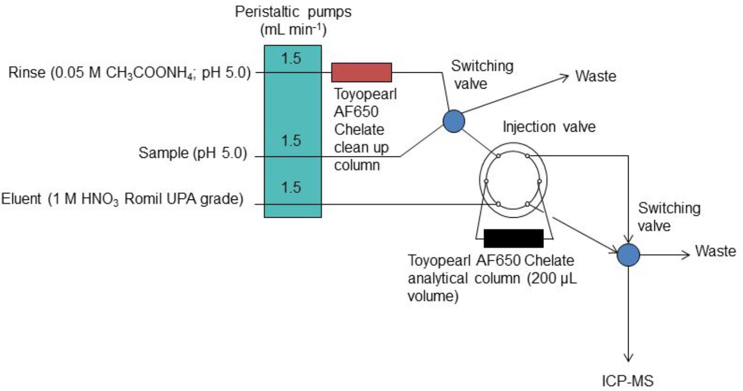
Figure 1. The FI manifold with on-line preconcentration and ICP-MS detection for the determination of iron in seawater. Reprinted from Clough et al. (2015). Uncertainty contributions to the measurement of dissolved Co, Fe, Pb, and V in seawater using flow injection with solid phase preconcentration and detection by collision cell – quadrupole ICP-MS, Copyright 2015, with permission from Elsevier (Clough et al., 2015).

FIGURE 2

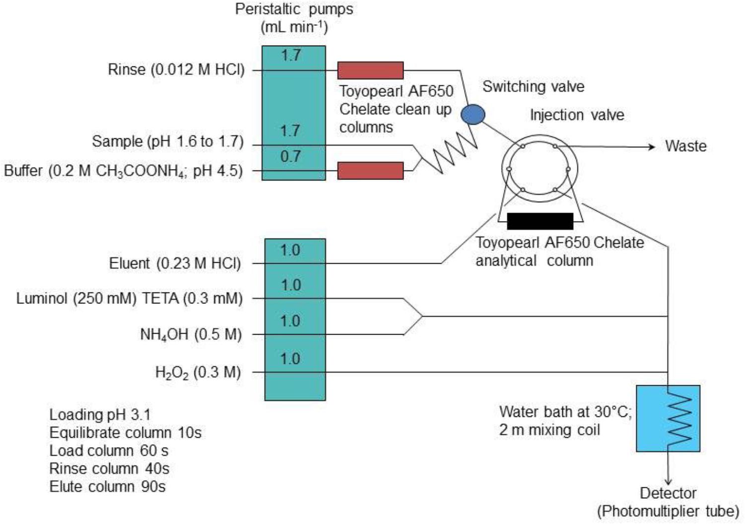
Figure 2. The FI manifold with on-line preconcentration and chemiluminescence detection for the determination of iron in seawater. Reprinted from Floor et al. (2015). Combined uncertainty estimation for the determination of the dissolved iron concentration in seawater using flow injection with chemiluminescence detection, Copyright 2015, with permission from Wiley Periodicals, Inc. on behalf of the Association for the Sciences of Limnology and Oceanography (Floor et al., 2015).

In the former example, the relative expanded uncertainty (U_{c_rel}) of each analytical result was estimated using the numerical differentiation method of Kragten (1994). This approach is easy to adopt and estimates the effect of each parameter in the measurement equation on the analytical result using a simple spreadsheet. Worked examples can be found in the Eurachem guide (Ellison and Williams, 2012), as well as on the website http://www.ut.ee/katsekoda/GUM_examples/. It is important to provide a clear statement of what is being measured (the measurand) and the measurement equation used to calculate the result. It should be stressed that the conversion of a signal to a concentration must be done carefully, taking into consideration (on a case by case basis) how to deal with non-zero intercepts and non-linear calibration curves. In the first example the measurands were the concentrations of dissolved cobalt, iron, lead and vanadium in seawater and the following equation was used as the model for calculating C_S (the analyte concentration in the sample);

$$C_S=\frac{\left(\frac{(I_S-I_{WB})\times V_1}{F}\right)-(B_C\times B_V)}{V_2}\mathrm{\hspace{0.17em}}\mathrm{\hspace{0.17em}}\mathrm{\hspace{0.17em}}\mathrm{\hspace{0.17em}}\mathrm{\hspace{0.17em}}\mathrm{\hspace{0.17em}}\mathrm{\hspace{0.17em}}\mathrm{\hspace{0.17em}}\mathrm{\hspace{0.17em}}\mathrm{\hspace{0.17em}}\mathrm{\hspace{0.17em}}\mathrm{\hspace{0.17em}}\mathrm{\hspace{0.17em}}\mathrm{\hspace{0.17em}}\mathrm{\hspace{0.17em}}\mathrm{\hspace{0.17em}}\mathrm{\hspace{0.17em}}\mathrm{\hspace{0.17em}}\mathrm{\hspace{0.17em}}\mathrm{\hspace{0.17em}}\mathrm{\hspace{0.17em}}\mathrm{\hspace{0.17em}}(1)$$

I_S = analyte signal (area measurement). The standard uncertainty for I_S was calculated from the peak area precision (n = 3).

I_WB = wash blank signal (area measurement). The standard uncertainty for I_WB was calculated from the peak area precision (n = 10).

V₁ = volume of the sample + added pH buffer solution. The standard uncertainty of V₁ was taken from the manufacturers certificates for the pipettes and plastic laboratory ware used.

F = slope of the calibration line (i.e., the sensitivity coefficient). The uncertainty of the slope of the calibration line was calculated using regression statistics (Miller and Miller, 2010) and assumed that systematic effects affecting all calibration line points in the same direction (e.g. standard substance purity) were negligible.

B_C = analyte concentration in the buffer solution. The standard uncertainty of B_C was taken as the standard deviation of five replicate measurements of the pH adjustment buffer.

B_V = volume of the buffer solution. The standard uncertainty of B_V was taken from the manufacturers certificates for the pipettes and plastic laboratory ware used.

V₂ = initial sample volume. The standard uncertainty of V₂ was taken from the manufacturers certificates for the pipettes and plastic laboratory ware used.

This approach does not take into account other potential systematic effects such as incomplete selectivity and analyte losses. Details of the analytical method can be found elsewhere (Clough et al., 2015).

The analytical figures of merit for the measurement of iron in three seawater RMs are shown in Table 1 and the relative uncertainty contributions of each parameter are given in Table 2. In summary, the relative expanded uncertainty (U_{c_rel}) for the concentration of iron in three RMs obtained by Clough et al. ranged from 8 to 18%, with the largest uncertainty associated with the lowest concentration (GEOTRACES GS; 0.50 nmol L^-1). For the GS RM, measurement of the sample peak area (I_S) was the major contributor to the overall uncertainty (73%), with lesser contributions from the slope of the calibration line (F; 8%) and the wash blank (I_WB; 17%). In this instance, a longer sample loading time could potentially lead to a lower uncertainty for I_s but the trade-off would be the time required for each analytical cycle. The certified concentration for the NASS-6 CRM is 9.64 nmol L^-1 and in this case the main contributor was the slope of the calibration line (81%), with lesser contributions from the sample peak area, due to the increase in signal intensity, and the wash blank.

TABLE 1

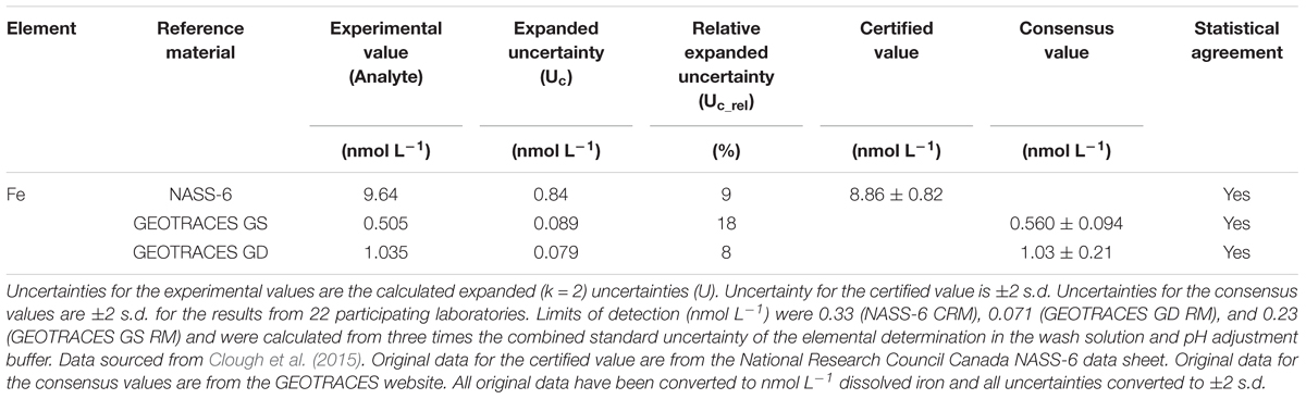
Table 1. Analytical data for the measurement of dissolved iron (nmol L^-1) in seawater using flow injection with ICP-MS detection.

TABLE 2

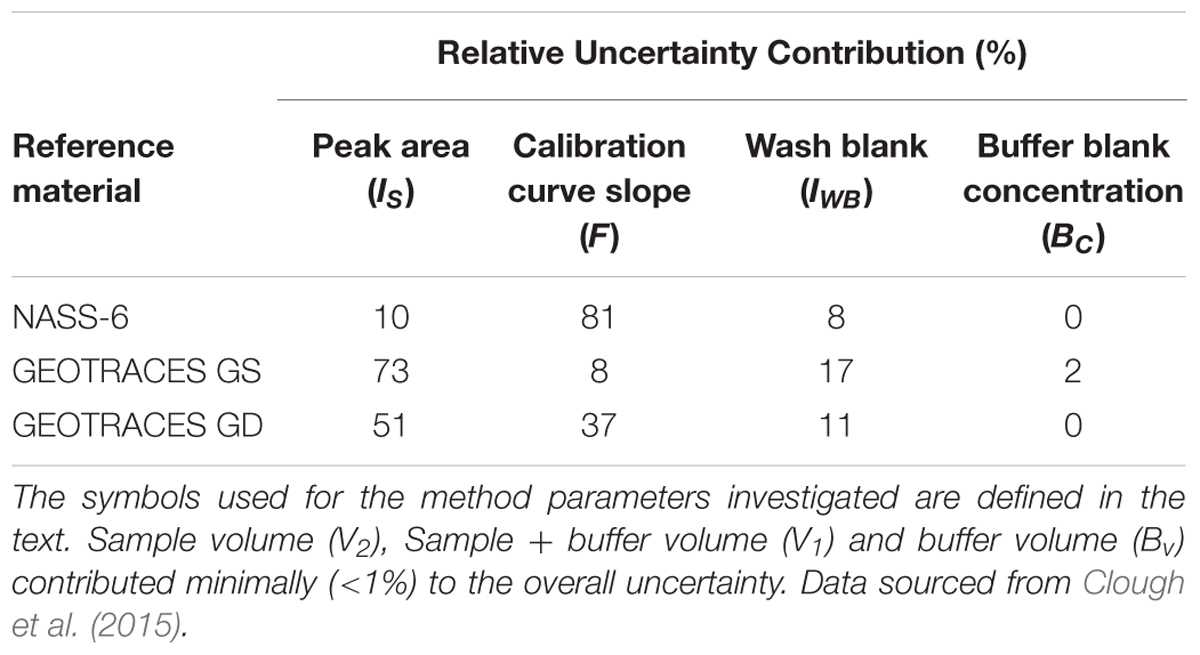
Table 2. Uncertainty contributions for the measurement of dissolved iron in seawater using flow injection with ICP-MS detection.

Whilst on-line preconcentration with ICP-MS detection is well suited to the determination of iron in seawater in the laboratory, and has the added benefit of simultaneous multi-element detection, it is not suitable for use on-board ship. For such applications, portable techniques such as flow injection with chemiluminescence detection (FI-CL) are preferred (Worsfold et al., 2014). The possible major sources of uncertainty for calculating C_S (the dissolved iron concentration in the sample in ng kg^-1) using this approach are shown in an Ishikawa diagram (Figure 3). The relative expanded uncertainty (U_{c_rel}) for the determination of iron in seawater using FI-CL has been rigorously assessed (Floor et al., 2015). The following equation incorporates all of the uncertainty components used in the model;

$$C_S=\frac{{\overline{I}}_{R\_S}\cdot {\mathrm{\delta }}_{rep\_S}\cdot {\mathrm{\delta }}_{stab\_S}\cdot {\mathrm{\delta }}_{WtoV\_S}-{\overline{I}}_{R\_B}\cdot {\mathrm{\delta }}_{stab\_B}\cdot {\mathrm{\delta }}_{rep\_B}\cdot {\mathrm{\delta }}_{matrix\_B}}{F_{reg}\cdot {\mathrm{\delta }}_{matrix\_std}}\mathrm{\hspace{0.17em}}\mathrm{\hspace{0.17em}}\mathrm{\hspace{0.17em}}\mathrm{\hspace{0.17em}}\mathrm{\hspace{0.17em}}\mathrm{\hspace{0.17em}}\mathrm{\hspace{0.17em}}\mathrm{\hspace{0.17em}}\mathrm{\hspace{0.17em}}\mathrm{\hspace{0.17em}}\mathrm{\hspace{0.17em}}(2)$$

Where R refers to the raw data, S refers to the sample, B refers to the blank and std refers to the calibration standard. δ terms are unity multiplicative correction factors carrying the relative uncertainty associated with the parameter considered. I is the analytical signal intensity (V) and F_reg is the sensitivity coefficient (slope, V L nmol^-1). rep is the uncertainty arising from the intensity repeatability, stab is the uncertainty arising from the intensity stability over an analytical sequence, WtoV is the uncertainty related to the difference in loaded mass of the analyte (whether it is done by weighing or volumetrically), and matrix is the uncertainty arising from matrix effects on the sensitivity. Whilst the nomenclature is different to that used in Equation 1, it has followed that used in the original publication. Further details of the analytical method can be found in Floor et al. (2015).

FIGURE 3

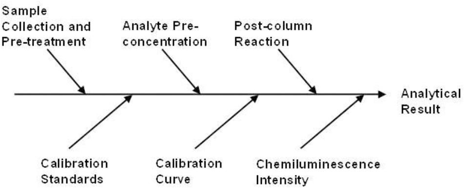
Figure 3. The possible major sources of uncertainty for calculating C_S (the dissolved iron concentration in the sample in ng kg^-1) using FI-CL. Reprinted from Worsfold et al. (2013). Flow injection analysis as a tool for enhancing oceanographic nutrient measurements – a review, Copyright 2013, with permission from Elsevier (Worsfold et al., 2013).

The analytical figures of merit for the measurement of iron with FI-CL in the GS and GD reference materials are shown in Table 3. The combined expanded relative uncertainty for the concentration of iron (U_{c_rel}) was ≈12% for peak height measurements and ≈10% for peak area measurements. Gravimetric loading gave a slightly lower combined uncertainty compared with volumetric loading (e.g., 12% cf. 13% for GD). RM results for GS and GD were in agreement with consensus values within uncertainty statements based on the methodology reported by Linsinger (2005) in ERM-1, free to download from https://ec.europa.eu/jrc/en/reference-materials/application-notes. For comparative purposes, the major relative uncertainty contributions for GD were the within-sequence-stability (intermediate precision; assessed by making 5 measurements, each of 6 replicates, over 32 h) at 22% and the sensitivity coefficient (slope of the calibration line) at 70%. The normalized signal intensity repeatability (i.e., the short term instrumental precision) accounted for only 7.9% of the total uncertainty and highlights the fact that reporting only the instrumental precision can seriously underestimate the overall uncertainty. Floor et al. (2015) therefore suggested that it is most beneficial to have a low uncertainty on the calibration slope and hence recommended the use of a sufficient number of standards (at least the non-spiked standard and 5 spiked levels) and replicate measurements of each (6). They also highlighted the importance of correctly estimating the within-sequence-stability, which should be done under the same measurement conditions as for the samples. They concluded that “Results obtained indicate that an uncertainty estimation based on the signal repeatability alone, as is often done in FI-CL studies, is not a realistic estimation of the overall uncertainty of the procedure.” (Floor et al., 2015).

TABLE 3

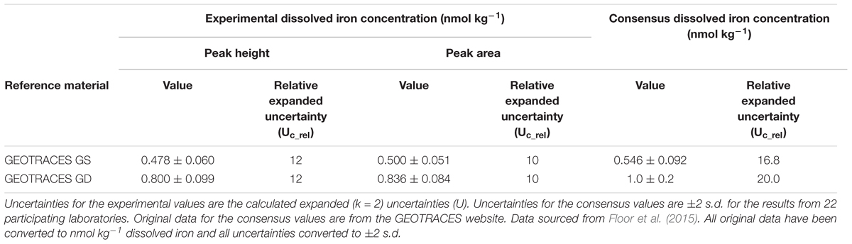
Table 3. Analytical data for the measurement of dissolved iron (nmol kg^-1) in seawater using FI-CL with gravimetric loading.

The Top-Down Approach

Many laboratories will have historical data on the intermediate precision and analytical bias of a method. These data can readily be used for the within-laboratory validation approach of measurement uncertainty estimation known as “top down.” Its best-known formalization is the Nordtest^TM approach (Magnusson et al., 2012) which uses the following equation:

$$u_c=\sqrt{(u\mathrm{\hspace{0.17em}}{(R_w)}^2+u\mathrm{\hspace{0.17em}}{(bias)}^2}\mathrm{\hspace{0.17em}}\mathrm{\hspace{0.17em}}\mathrm{\hspace{0.17em}}\mathrm{\hspace{0.17em}}\mathrm{\hspace{0.17em}}\mathrm{\hspace{0.17em}}\mathrm{\hspace{0.17em}}\mathrm{\hspace{0.17em}}\mathrm{\hspace{0.17em}}\mathrm{\hspace{0.17em}}\mathrm{\hspace{0.17em}}\mathrm{\hspace{0.17em}}\mathrm{\hspace{0.17em}}\mathrm{\hspace{0.17em}}\mathrm{\hspace{0.17em}}\mathrm{\hspace{0.17em}}\mathrm{\hspace{0.17em}}\mathrm{\hspace{0.17em}}\mathrm{\hspace{0.17em}}\mathrm{\hspace{0.17em}}\mathrm{\hspace{0.17em}}\mathrm{\hspace{0.17em}}\mathrm{\hspace{0.17em}}\mathrm{\hspace{0.17em}}\mathrm{\hspace{0.17em}}(3)$$

Where u_c is the combined standard uncertainty (approximates to a 68.3% confidence interval), u(R_w) is the uncertainty estimate of intermediate precision (random effects) and u(bias) is the uncertainty estimate of possible laboratory and procedural bias (systematic effects). This approach therefore combines the uncertainties associated with day to day reproducibility and possible bias in the complete data set and is easy to use. For analytical methods that are routinely used, laboratories will have access to the information required to calculate u_c from archived quality assurance data.

If a laboratory is implementing a new method it is best to start with a limited objective but new data should be added regularly. So, an intermediate precision value obtained from data collected over 4 weeks is not sufficient; data should be collected over several months and preferably over at least 1 year (Magnusson et al., 2012) and data from the analysis of just one CRM is generally not enough for bias evaluation. However, limited data (e.g., intermediate precision data from 4 weeks and bias estimate from one CRM) can be used as a first approximation. Intermediate precision can be recalculated using longer time intervals, bias can be re-estimated using several reference values and the measurement uncertainty estimate can then be recalculated. Constant improvement in the quality and amount of data is therefore the key to producing reliable analytical results and robust uncertainty estimations.

Several examples of the application of the Nordtest^TM approach to analytical datasets can be found at http://www.ut.ee/katsekoda/GUM_examples/, including annotated Excel files. The example of most relevance to the oceanographic community estimates the uncertainty associated with the determination of aluminum, vanadium, iron and cadmium in marine suspended particles using ICP-MS detection. Replicate measurements were performed over 10 months using a plankton matrix CRM. All of the method steps, including sample preparation and ICP-MS determination, were carried out on each day of analysis using a method detailed in Milne et al. (2017) which was a modification of a previously published method (Ohnemus et al., 2014). The random uncertainty component was evaluated via intermediate precision and the systematic component was evaluated using the found and certified values of the CRM. Relative expanded uncertainties (U_{c_rel}) ranged from 16 to 30% (see the Excel file provided in Supplementary Material S1 for further details). A similar approach was used by Rapp et al. to calculate the relative expanded uncertainties (U_{c_rel}), which ranged from 13 to 25%, for the determination of Cd, Co, Cu, Fe, Mn, Ni, Pb, and Zn in seawater by on-line preconcentration and high-resolution sector field ICP-MS detection (Rapp et al., 2017).

The example discussed in more detail in this article uses the same FI-CL manifold (with minor modifications) for the measurement of iron in seawater as was used for the second “bottom up” example (Floor et al., 2015) and therefore provides a direct comparison of the results from the two approaches to uncertainty estimation. The minor manifold differences were a loading pH of 3.5–3.7 (rather than 3.1), a column rinse time of 20 s (rather than 40 s ), flow rates for the sample and rinse lines of 1.5 mL min^-1 (rather than 1.7 mL min^-1) and flow rate for the buffer line of 0.6 mL min^-1 (rather than 0.7 mL min^-1).

The blank signal associated with the eluent and post-preconcentration column reagents was included in the baseline; therefore if any blank signal was detected it would likely have been from the ammonium acetate buffer, HCl wash and/or the manifold. The blank contribution from these potential sources, determined by shutting off the sample line and loading only buffer, were typically below the limit of detection. This showed that the clean-up columns effectively removed any contribution from the buffer and wash solutions and that the cleaning procedures used helped to maintain a trace metal clean manifold. Further blank contributions could have arisen due to the manipulation of samples e.g., by the addition of H₂O₂ or HCl, but such contributions are negligible if highly pure reagents are used (Bowie et al., 2004; Klunder et al., 2011).

The accuracy of this method was evaluated using SAFe D1, D2 (deep water) and S (surface water) RMs and the NASS-5 CRM. The results were in agreement with consensus/certified values within uncertainty statements (Linsinger, 2005) as shown in Table 4. Due to the limited quantity of these materials available, internal quality control standards were developed and run daily to assess reproducibility; the results obtained for both the consensus material and the internal quality control standards were then used to calculate a combined uncertainty estimate.

TABLE 4

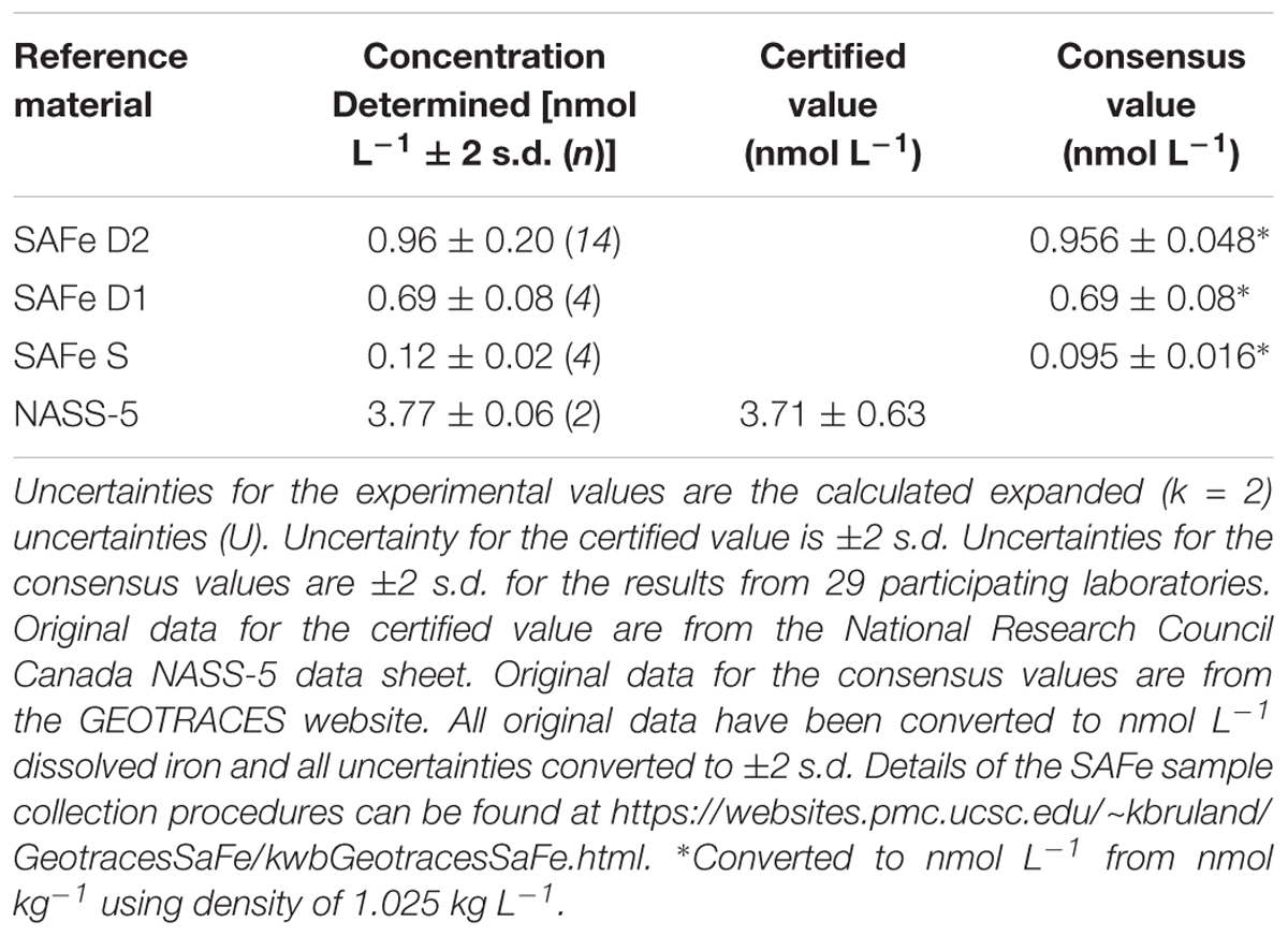
Table 4. Validation of the FI-CL method, with the dissolved iron concentrations determined for the consensus/reference materials in nmol L^-1.

In this example the dataset was comprised of ≈2 years of analyses, enabling a more robust estimate of the analytical uncertainty than the short term internal instrumental precision associated with replicate measurements of a single sample (typically <5%). Both RMs with consensus values and internal quality control materials (open ocean seawater with dissolved iron concentrations in the range 0.69 – 1.49 nmol L^-1) were used to calculate a “top down” estimate of the combined measurement uncertainty using the Nordtest^TM approach. The calculated relative combined standard uncertainty (u_{c_rel}) was 9.5% and hence the relative expanded uncertainty (U_{c_rel}) was 18.9%. For further details see the Excel file provided in Supplementary Material S2. This uncertainty estimate compares well with a “bottom up” assessment (Floor et al., 2015). Further examination of the combined uncertainty estimate shows that within laboratory reproducibility (u(R_w)_rel) contributed 65% of the analytical uncertainty, with 35% coming from possible laboratory and procedural bias (u(bias)_rel). The work of Floor et al. (2015) suggests the main reason for the uncertainty contribution from the within laboratory reproducibility is likely to be associated with the calibration slope for the FI-CL method.

The contribution from possible laboratory and procedural bias includes the uncertainty of the published consensus concentrations [e.g., SAFe D2 0.956 ± 0.024 nmol L^-1 (1 s.d.)] and the possible bias estimated from the differences between the published mean concentrations and those determined in the course of the analysis reported here (see Supplementary Material S2). The results of the estimate indicated that the uncertainty associated with the published consensus concentrations (u(C_ref)_rel) contributed 86% of the uncertainty associated with possible laboratory and procedural bias. This is an important point as it shows, for this particular example, that any reduction in the bias of the analysis would have minimal impact on the combined expanded uncertainty (U_c).

The iron concentration of seawater samples, particularly from transects running from coastal, through shelf to open ocean waters, can span several orders of magnitude (<0.1 to >100 nmol L^-1 for filtered and unfiltered samples) (Birchill et al., 2017) and the available RMs cover a narrow range of iron concentrations (see e.g., the concentrations of the GEOTRACES and SAFe reference materials). Hence the combined uncertainty estimates obtained using these reference materials would not be applicable over the entire concentration range, even if uncertainty calculations were carried out with relative quantities. Therefore, data for the SAFe S reference material (0.12 ± 0.02 nmol L^-1) shown in Supplementary Material S2 used the short term uncertainty associated with replicate measurements, as is common practice. An assessment of the within laboratory reproducibility can be estimated using in house quality control material. At lower concentrations, e.g., close to the limit of detection, the relative uncertainty increases and hence it is generally recommended that absolute values are used for sample concentrations near the limit of detection when using the Nordtest^TM. The decision on the threshold for using absolute values should be made based on experience rather than a mathematical algorithm. Using this approach the relative expanded uncertainty (U_{c_rel}) for iron concentrations in seawater was 14% (for 4 – 16 nmol L^-1 Fe) and 4% for 49 – 70 nmol L^-1 Fe and the expanded uncertainty (U_c) was 0.04 nmol L^-1 for 0.14 – 0.24 nmol L^-1 Fe.

Conclusion and Recommendations

Quantifying the concentration of iron in seawater is undoubtedly challenging, particularly when one considers the different physical and chemical forms of the element and the complexity of the sample matrix. It is therefore imperative that results for the measurement of iron (and other trace elements) are accompanied by a realistic assessment of uncertainty. It is common practice to state an uncertainty based on the internal instrumental precision of replicate measurements of a sample using the method of choice. However, a more holistic and robust approach that considers all of the factors contributing to the overall uncertainty provides a more realistic evaluation. This in turn aids interpretation of oceanographic measurements that are used to elucidate biogeochemical cycles and provide input data for oceanographic models.

The two approaches described in this paper are the “bottom up” or modeling approach and the “top down” or empirical approach. The former (“bottom up”) is a more rigorous but time consuming approach and is therefore not practical for many laboratories. However, it has the advantage of providing information on the relative contributions of the different factors to the overall uncertainty. This information is very useful for method development as it pinpoints which factors make the largest contribution and should therefore be targeted for improvement. The latter (“top down”) is easier to apply but does require long term data from the analysis of reference materials. It is important to emphasize, however, that many laboratories will already have the necessary information from archived quality assurance data to use the Nordtest^TM approach to calculate the combined uncertainty. Furthermore, this spreadsheet based approach is very easy to use.

The uncertainties reported for the determination of iron in seawater using FI-CL show good agreement between the two approaches and suggest that a relative expanded uncertainty (U_{c_rel}) of around 10 – 20% is the best that can be achieved, depending on the sample concentration. These values provide a more realistic estimation of uncertainty than values of ≤5% that are typically reported for the short term instrumental precision. For further guidance on the estimation of measurement uncertainty in chemical analysis the reader is referred to an on-line course at https://sisu.ut.ee/measurement/uncertainty.

Author Contributions

PW, EA, ML, and SU were co-investigators for the project. IL was a contributor to the project. AB, RC, and AM provided data for the case studies. All authors were involved in the preparation and editing of the manuscript.

Funding

This paper was supported by funding from the European Union’s Horizon 2020 Research and Innovation Program under the AtlantOS program, grant agreement No. 633211. AM and AB were supported by funding from the UK Natural Environment Research Council under grants NE/K001779/1 and NE/L501840/1, respectively.

Conflict of Interest Statement

The authors declare that the research was conducted in the absence of any commercial or financial relationships that could be construed as a potential conflict of interest.

The handling Editor declared a shared affiliation, though no other collaboration, with one of the authors EA at time of review.

Supplementary Material

The Supplementary Material for this article can be found online at: https://www.frontiersin.org/articles/10.3389/fmars.2018.00515/full#supplementary-material

Footnotes

1. ^http://www.goosocean.org/
2. ^https://www.atlantos-h2020.eu/
3. ^http://hahana.soest.hawaii.edu/hot/methods/results.html
4. ^http://www.geotraces.org/sic/intercalibrate-data/cookbook
5. ^http://www.geotraces.org/
6. ^https://sisu.ut.ee/measurement/uncertainty

References

Bewers, J. M., Dalziel, J., Yeats, P. A., and Barron, J. L. (1981). An intercalibration for trace-metals in seawater. Mar. Chem. 10, 173–193. doi: 10.1016/0304-4203(81)90040-2

CrossRef Full Text | Google Scholar

Birchill, A. J., Milne, A., Woodward, E. M. S., Harris, C., Annett, A., Rusiecka, D., et al. (2017). Seasonal iron depletion in temperate shelf seas. Geophys. Res. Lett. 44, 8987–8996. doi: 10.1002/2017gl073881

CrossRef Full Text | Google Scholar

Bowie, A. R., Achterberg, E. P., Blain, S., Boye, M., Croot, P. L., de Baar, H. J. W., et al. (2003). Shipboard analytical intercomparison of dissolved iron in surface waters along a north-south transect of the Atlantic Ocean. Mar. Chem. 84, 19–34. doi: 10.1016/S0304-4203(03)00091-4

CrossRef Full Text | Google Scholar

Bowie, A. R., Achterberg, E. P., Croot, P. L., de Baar, H. J. W., Laan, P., Moffett, J. W., et al. (2006). A community-wide intercomparison exercise for the determination of dissolved iron in seawater. Mar. Chem. 98, 81–99. doi: 10.1016/j.marchem.2005.07.002

CrossRef Full Text | Google Scholar

Bowie, A. R., Sedwick, P. N., and Worsfold, P. J. (2004). Analytical intercomparison between flow injection-chemiluminescence and flow injection-spectrophotometry for the determination of picomolar concentrations of iron in seawater. Limnol. Oceanogr. Methods 2, 42–54. doi: 10.4319/lom.2004.2.42

CrossRef Full Text | Google Scholar

Clough, R., Floor, G. H., Quétel, C. R., Milne, A., Lohan, M. C., and Worsfold, P. J. (2016). Measurement uncertainty associated with shipboard sample collection and filtration for the determination of the concentration of iron in seawater. Anal. Methods 8, 6711–6719. doi: 10.1039/c6ay01551d

CrossRef Full Text | Google Scholar

Clough, R., Sela, H., Milne, A., Lohan, M. C., Tokalioglu, S., and Worsfold, P. J. (2015). Uncertainty contributions to the measurement of dissolved Co, Fe, Pb and V in seawater using flow injection with solid phase preconcentration and detection by collision/reaction cell - Quadrupole ICP-MS. Talanta 133, 162–169. doi: 10.1016/j.talanta.2014.08.045

PubMed Abstract | CrossRef Full Text | Google Scholar

Cutter, G. A. (2013). Intercalibration in chemical oceanography-getting the right number. Limnol. Oceanogr. Methods 11, 418–424. doi: 10.4319/lom.2013.11.418

CrossRef Full Text | Google Scholar

Ellison, S. L. R., and Williams, A. (eds) (2012). Eurachem/CITAC guide: Quantifying Uncertainty in Analytical Measurement. Available at: http://www.eurachem.org

Google Scholar

Floor, G. H., Clough, R., Lohan, M. C., Ussher, S. J., Worsfold, P. J., and Quétel, C. R. (2015). Combined uncertainty estimation for the determination of the dissolved iron amount content in seawater using flow injection with chemiluminescence detection. Limnol. Oceanogr. Methods 13, 673–686. doi: 10.1002/lom3.10057

PubMed Abstract | CrossRef Full Text | Google Scholar

Hood, E. M., Sabine, C. L., and Sloyan, B. M. (2010). The GO-SHIP Repeat Hydrography Manual: A Collection of Expert Reports and Guidelines, IOCCP Report Number 14, ICPO Publication Series Number 134. http://www.go-ship.org/HydroMan.html

Google Scholar

Intergovernmental Panel on Climate Change [IPCC]. (2013). “Climate change 2013: the physical science basis,” in Contribution of Working Group I to the Fifth Assessment Report of the Intergovernmental Panel on Climate Change, eds T. F. Stocker, D. Qin, G.-K. Plattner, M. Tignor, S. K. Allen, J. Boschung, et al. (Cambridge, UK: Cambridge University Press).

Google Scholar

International Organization for Standardization/International Electrotechnical Commission [ISO/IEC]. (2005). General Requirements for the Competence of Testing and Calibration Laboratories. Geneva: International organization for standardization/international electrotechnical commission.

Google Scholar

Johnson, K. S., Boyle, E., Bruland, K., Coale, K., Measures, C., Moffett, J., et al. (2007). Developing standards for dissolved iron in seawater. EOS 88, 131–132. doi: 10.1029/2007EO110003

CrossRef Full Text | Google Scholar

Klunder, M. B., Laan, P., Middag, R., De Baar, H. J. W., and van Ooijen, J. C. (2011). Dissolved iron in the southern ocean (Atlantic sector). Deep Sea Res. Part II Top. Stud. Oceanogr. 58, 2678–2694. doi: 10.1016/j.dsr2.2010.10.042

CrossRef Full Text | Google Scholar

Knap, A. H., Michaels, A. F., Steinberg, D., Bahr, F., Bates, N., Bell, S., et al. (1997). BATS Methods Manual. Woods Hole: U.S. JGOFS Planning Office.

Google Scholar

Kragten, J. (1994). Tutorial review. Calculating standard deviations and confidence intervals with a universally applicable spreadsheet technique. Analyst 119, 2161–2165. doi: 10.1039/an9941902161

CrossRef Full Text | Google Scholar

Landing, W. M., Cutter, G. A., Dalziel, J. A., Flegal, A. R., Powell, R. T., Schmidt, D., et al. (1995). Analytical intercomparison results from the 1990 intergovernmental-oceanographic-commission open-ocean base-line survey for trace-metals - atlantic-ocean. Mar. Chem. 49, 253–265. doi: 10.1016/0304-4203(95)00016-K

CrossRef Full Text | Google Scholar

Linsinger, T. (2005). Comparison of a Measurement Result with the Certified Value, European Commission - Joint Research Centre (IRMM), Geel, Belgium. Geel: European Commission - Joint Research Centre (IRMM).

Google Scholar

Magnusson, B., Näykki, T., Hovind, H., and Krysell, M. (2012). Handbook for Calculation of Measurement Uncertainty in Environmental Laboratories, 3rd Edn. Available at: http://www.nordtest.info

Google Scholar

Miller, J. N., and Miller, J. C. (2010). Statistics and Chemometrics for Analytical Chemistry. London: Pearson Education.

Google Scholar

Milne, A., Schlosser, C., Wake, B. D., Achterberg, E. P., Chance, R., Baker, A. R., et al. (2017). Particulate phases are key in controlling dissolved iron concentrations in the (sub)tropical North Atlantic. Geophys. Res. Lett. 44, 2377–2387. doi: 10.1002/2016GL072314

CrossRef Full Text | Google Scholar

Ohnemus, D. C., Auro, M. E., Sherrell, R. M., Lagerström, M., Morton, P. L., Twining, B. S., et al. (2014). Laboratory intercomparison of marine particulate digestions including Piranha: a novel chemical method for dissolution of polyethersulfone filters. Limnol. Oceanogr. Methods 12, 530–547. doi: 10.4319/lom.2014.12.530

CrossRef Full Text | Google Scholar

Rapp, I., Schlosser, C., Rusiecka, D., Gledhill, M., and Achterberg, E. P. (2017). Automated preconcentration of Fe, Zn, Cu, Ni, Cd, Pb, Co, and Mn in seawater with analysis using high-resolution sector field inductively-coupled plasma mass spectrometry. Anal. Chim. Acta 976, 1–13. doi: 10.1016/j.aca.2017.05.008

PubMed Abstract | CrossRef Full Text | Google Scholar

Rigaud, S., Puigcorbé, V., Cámara-Mor, P., Casacuberta, N., Roca-Martí, M., Garcia-Orellana, J., et al. (2013). A methods assessment and recommendations for improving calculations and reducing uncertainties in the determination of 210Po and 210Pb activities in seawater. Limnol. Oceanogr. Methods 11, 561–571. doi: 10.4319/lom.2013.11.561

CrossRef Full Text | Google Scholar

Worsfold, P. J., Clough, R., Lohan, M. C., Monbet, P., Ellis, P. S., Quetel, C. R., et al. (2013). Flow injection analysis as a tool for enhancing oceanographic nutrient measurements–a review. Anal. Chim. Acta 803, 15–40. doi: 10.1016/j.aca.2013.06.015

PubMed Abstract | CrossRef Full Text | Google Scholar

Worsfold, P. J., Lohan, M. C., Ussher, S. J., and Bowie, A. R. (2014). Determination of dissolved iron in seawater: a historical review. Mar. Chem. 166, 25–35. doi: 10.1016/j.marchem.2014.08.009

CrossRef Full Text | Google Scholar