The Kelp Cultivation Potential in Coastal and Offshore Regions of Norway

Introduction

In order to meet the future challenges of limited terrestrial food resources, a greater part of the human food consumption will need to be based on marine production, at lower trophic levels than today (Olsen, 2011). The demand for marine biomass for other purposes, such as biofuels, feed for animals, cosmetics, medicines, pharmaceuticals and raw materials for the biotechnological industry, is also expected to increase (Holdt and Kraan, 2011; Kraan, 2016).

Macroalgae are, by volume, the largest group of species in aquaculture, with a global production of 2.94 × 10⁷ tons wet weight per year (FAO, 2018). More than 99.9% of this is produced in Asia (Ibid.), but the interest in macroalgal aquaculture in the Western hemisphere is increasing. It has been suggested that by 2050, the value of the kelp industry may have a turnover of 4 × 10⁹ Euro per year in Norway alone, with a production of 2 × 10⁷ t per year (Olafsen et al., 2012). Globally, the potential for marine macroalgal cultivation has been suggested to lie at 10⁹ to 10¹¹ t dry weight (DW) (Lehahn et al., 2016).

There are many sectors and interests competing for space in coastal regions (Hersoug, 2013), including cultivation of macroalgae (Duarte et al., 2017). In order to manage the coastal zone, tools that can assess the suitability of different locations for different purposes are necessary. In order to grant aquaculture permits for macroalgae production, knowledge of the production potential and spatially explicit maps of suitable areas for production are needed. These maps must be based on physical, biological and biogeochemical variables important for the survival and growth of macroalgae. While most naturally growing macroalgae depend on some form of solid substrate and therefore grow mostly on the bottom as deep as the light penetration allows, macroalgal cultivation facilities may in principle be sited regardless of the seabed depth. This allows for great possibilities in the choice of cultivation sites and fewer direct conflicts with natural macroalgal communities.

Kelps are among the most important macroalgae in aquaculture. The main environmental variables for the growth of kelps are nutrients, light, temperature, and ocean currents (Wiencke and Bischof, 2012). For naturally growing kelps, wave exposure is also important, since waves keep the fronds free from sedimentation and epiphytic growth, while maximizing the light trapping area and sustaining a good flux of nutrients.

Biogeochemical conditions are determined by physical factors. The Norwegian Coastal Current (NCC) is one of the main physical drivers of the Norwegian coastal ecosystem. The NCC is driven by the outflow from the Baltic Sea and transports water northward along the Norwegian coast where it gets replenished with freshwater and nutrients from rivers and fjords along the way (Sætre, 2007). This leads to periods of strong stratification, especially in fjords and in the NCC itself, and thus to nutrient depletion in the surface layer in spring/early summer following the pelagic spring bloom. This has implications for the nutrients available for macroalgal primary production.

The main objective of the present paper was to investigate how the aquaculture production potential for the commercially important kelp species Saccharina latissima varies along and outside the Norwegian coast. While there have been many surveys on the production and biomass in natural kelp forests in Norway (Abdullah and Fredriksen, 2004; Moy et al., 2009; Gundersen et al., 2012), information on the cultivation potential for kelps outside natural kelp forests is largely missing on a coastal scale. In absence of large, high resolution data sets on industrial cultivation yields, a coupled hydrodynamic-biogeochemical ocean model system (SINMOD; Wassmann et al., 2006) was used. The model has been further coupled with an individual based growth model for S. latissima (Broch et al., 2013; Fossberg et al., 2018). Although dynamical modeling can never replace field experiments and surveys, the simulations provide results resolved in time and space that are especially useful in “data poor” contexts. Thus, both geographic and seasonal/interannual variations in the cultivation potential are considered, in addition to how these interplay with hydrographic and biogeochemical variables. In particular, nearshore to offshore and latitudinal gradients in the production yields and timing are considered. The simulation results on S. latissima frond sizes, a proxy for the biomass production potential, are compared with results from both cultivation experiments with S. latissima and surveys of the density of natural kelp populations in order to provide an evaluation of the realism of the results.

Materials and Methods

Coupled Hydrodynamic-Ecosystem-Kelp Model System (SINMOD)

Model Description

SINMOD is a coupled 3 dimensional hydrodynamic-biogeochemical model system (Slagstad and McClimans, 2005). The biogeochemical component includes compartments for, e.g., concentrations of nitrate (${\text{NO}}_3^{-}$), ammonium (${\text{NH}}_4^{+}$), silicate, detritus, bacteria, phytoplankton, ciliates and zooplankton (Wassmann et al., 2006). Phytoplankton production and nutrient uptake are calculated as combined effects of temperature, light, and nutrient concentrations. The phytoplankton is grazed by ciliates and zooplankton, and dead/respired matter enter the detritus and ammonium compartments and are further remineralized into nitrate and silicate. The attenuation of light is calculated from the background attenuation of the sea water and the concentration of phytoplankton. The details are given in Wassmann et al. (2006).

An individual based growth model for sugar kelp has been developed and coupled with SINMOD (Broch and Slagstad, 2012; Broch et al., 2013; Fossberg et al., 2018). The state variables in the growth model are frond area (A, unit: cm²), internal nitrogen reserves (N, unit: g N (g structural mass)⁻¹), and internal carbon reserves (C, unit: g C (g structural mass)⁻¹). The environmental variables used to force kelp growth in the model are temperature, salinity, light intensity (PAR), nutrient (${\text{NO}}_3^{-}$, ${\text{NO}}_4^{+}$) concentrations, water current speed and latitude (implicitly through the day length) (Broch and Slagstad, 2012; Broch et al., 2013; Fossberg et al., 2018) (Figure 1). Salinities below 25 PSU are assumed to cause reduced growth, nutrient uptake and photosynthetic rates (Bartsch et al., 2008; Mortensen, 2017). This effect has been introduced in the model by multiplying those rates by the factor

$f_{\text{salinity}}=\{\begin{array}{ll}1,& \text{for }S\ge 25\\ 1+\frac{S-25}{18},& \text{for }16\le S<25\\ \frac{S}{32},& \text{for }0\le S<16\end{array}$

where S denotes the salinity (PSU).

FIGURE 1

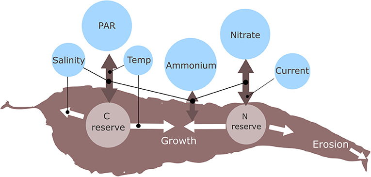
Figure 1. Schematic for the main processes in the kelp growth model and how the state variables are linked with the environmental variables simulated by the 3D ocean model.

The effect of water current speed has been modified from that in Broch et al. (2013). In the present version, the uptake rate of nutrients, J, is calculated as

$\begin{array}{l}J=f_{\mathrm{\text{current}}}{J}_N\end{array}$

where J_N is the uptake rate per unit frond area based on external and internal nutrient reserves, and the water current speed, U (ms⁻¹), is taken into account by the factor

$\begin{array}{l}{f}_{\mathrm{\text{current}}}(U)=a(1-e^{-U/U_0})+b,\end{array}$

with a = 0.72, b = 0.28, and U₀ = 0.045 ms⁻¹ (Hurd et al., 1996; Broch and Slagstad, 2012). The additional constant term b ensures a substantial nutrient uptake even for very low current speeds (Broch et al., 2013). The numerical values of the parameters have been chosen such that f _current(0.03) = 0.63 (Hurd et al., 1996; Broch and Slagstad, 2012).

The effect of day lengths and changes in day length is accounted for using Broch and Slagstad (2012). For latitudes L above the polar circle (>66.5 °N) a modified version of the photoperiod effect f _photo at Julian day number n is applied as follows:

$\begin{array}{l}{f}_{\mathrm{\text{photo}}}(n,L)=0.85(1+\delta (n,L))+0.3,L>66.5,\end{array}$

where

$\delta \left(n,L\right)=\{\begin{array}{c}0, \lambda \left(n,L\right)=0 \\ \text{sgn}(\lambda \left(n,l\right), \lambda (n.L)\ne 0 \end{array}.$

Here, λ(n, L) denotes the normalized change in day length at day number n and latitude L. See Figure 2.

FIGURE 2

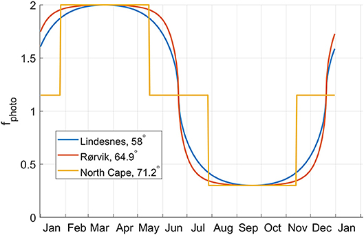
Figure 2. The growth rate modifier f _photo, taking into account the effect of changes in the day length, plotted as a function of the day in the year for three latitudes.

Model Simulations

Four SINMOD model domains with 800 m horizontal resolution, together covering the entire Norwegian coast, were used. The model was nested from a 20 km model setup (Wassmann et al., 2006) to a setup of 4 km horizontal resolution for the Northeastern Atlantic, and finally to the 800 m resolution model domains (Figure 3). Vertical layers of thickness ranging from 3 m near the surface to 50–100 m at greater depths were used. The bathymetry data for the model domains was provided by the Norwegian Mapping Authority (www.kartverket.no) with additional data from IBCAO (www.ibcao.org).

FIGURE 3

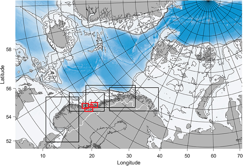
Figure 3. The model domain for the Nordic Seas in 4 km horizontal resolution used to produce boundary conditions for the coastal models. The coastal model domains in 800 m horizontal resolution are outlined by the black rectangles, while the 160 m model domains are outlined in red. The thin black curves are 200, 500, and 1,000 m isobaths.

The 20 km model was forced by tidal components M₂, S₂, K₁, and N₂ at the open boundaries with data on global ocean tides imported from the TPXO 6.2 model (http://www.coas.oregonstate.edu/research/po/research/tide/global.html). ERA-Interim data from ECMWF (Dee et al., 2011) were used for atmospheric forcing. Data on freshwater discharges from rivers and land were collected from simulations by the Norwegian Water Resources and Energy Directorate (www.nve.no). The simulations were performed using a version of the HBV-model in 1 km horizontal resolution (Beldring et al., 2003).

The simulation time steps used in the 800 m simulations were 72 and 120 s, depending on horizontal resolution and bathymetry via standard numerical stability criteria.

The simulations using the 800 m models were run for a period of 4 entire growth seasons, from autumn 2012 until summer 2016. The 20/4 km models were subjected to a spin up period of ~20 years prior to the simulation start.

For each growth season, each grid cell down to 8 m depth was initialized with the same kelp state variable values at the deployment dates. The initial values used were

• A(0) = 0.2 cm²,

• N(0) = 0.02, and

• C(0) = 0.4,

as in Broch et al. (2013). For all the model domains and cultivation cycles, deployments in late summer (September) and winter (February) were assumed.

For the county of Trøndelag, Central Norway, model setups of 160 m horizontal resolution were used to provide results in higher resolution for the cultivation season February-June. The 160 m models were nested from the 800 model for Central Norway (Figure 3). The setup and procedure was identical to that for the 800 m models except that atmospheric input from a high resolution setup of WRF (https://www.mmm.ucar.edu/weather-research-and-forecasting-model) was used instead of the ECMWF-data in order to include finer scale topographic effects close to land.

Comparing Simulation Results With Cultivation and Survey Data on S. latissima

Two complementary methods for evaluating the model performance were applied. The first (section Cultivation trials below) compared the simulated frond area of sugar kelp with measured averages from five cultivation trials in Central Norway. The second (section Field surveys of natural populations below) related the simulation results on kelp cultivation potential to the field observed coverage of naturally growing sugar kelp.

Cultivation Trials

Five cultivation trials were conducted at different locations in Central Norway in 2011–2016. Seedlings with a size of 1–5 mm length were produced from spores seeded either directly on 6 mm carrier ropes or on 1.2 mm twines that were twisted on 16 mm carrier ropes at sea deployment, following the protocol by Forbord et al. (2018). The growth was assessed regularly by measurement of the length and width of the fronds (n = 60–200). The average values of frond areas, calculated as A = 0.75 L W (Broch et al., 2013; Foldal, 2018) from the experiments, were compared with the simulation results from the 160 m resolution models for 2016 at the five locations. Simulated deployment dates were taken to the closest first of the month. The spatial variability in the simulation results was evaluated by considering also the minimum and maximum simulated frond areas from the 3 × 3 nearest model grid cells to the one matching the cultivation locations.

Field Surveys of Natural Populations

Wild sugar kelp coverage data were collected from the coast of Southern Norway, covering the coastal regions of the southern Norwegian Sea, the North Sea and the Skagerrak (Figure 4). Coverage was recorded using an underwater video camera and georeferencing of stations at which coverage was defined semi-quantitatively at a five-step scale: 0 (absent), 1 (single individuals), 2 (scarce, i.e., a few individuals), 3 (common/moderately dense, i.e., many plants, but not a completely dense canopy cover), or 4 (dominating, i.e., a completely dense canopy cover). The data on kelp coverage was collected through the National program for mapping biodiversity (Bekkby et al., 2013), the sugar kelp monitoring program (Moy et al., 2009), the SaccRef sugar kelp research project (Gundersen et al., 2012), and the coastal monitoring program (e.g., Dale et al., 2018; Fagerli et al., 2018).

FIGURE 4

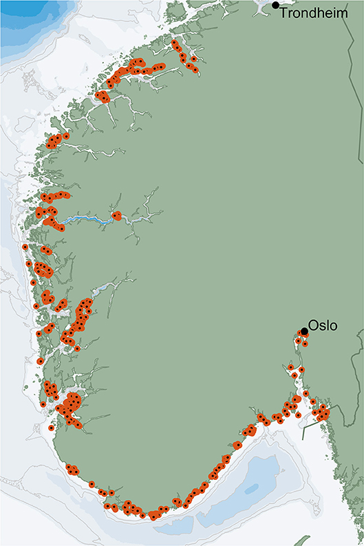
Figure 4. Locations for field survey data of wild sugar kelp population (S. latissima) coverage in southern Norway.

Simulation results from SINMOD using the southernmost model domain in Figure 3 for 2013, 2014, 2015, and 2016 were compared with the survey data on sugar kelp coverage. The basis for comparison was the frond area computed by the model from September to June. The frond area is the main structural variable in the kelp model and the variable that corresponds most closely to the kelp coverage observed in field surveys. For each survey data point the average simulated frond area in the 3 × 3 model grid cells in SINMOD, at a position and depth corresponding to the field survey data point, was used. The bottom layer was used whenever the model depth was less than the actual depth. The 3 × 3 arrays were used because the exact position might potentially be represented by a “land point” in the model and in order to reduce the effect of local variability in the model. Whenever all 9 cells were land cells, the entire survey data point was excluded from the comparison.

Evaluation of the Cultivation Potential

The simulation results were used to evaluate the cultivation potential for S. latissima in two different ways, by calculating a spatial “index” for the cultivation potential and by upscaling the biomass yield from individual level to large scale yields per unit area.

Spatial Index

The spatial index provides a means for comparison of the simulated kelp cultivation potentials at different locations, represented here by the different model grid cells, without considering the absolute yields. This is a comparison of the basic cultivation potential disregarding variables such as the choice of cultivation technology, farm sizes, or seeding density. It is calculated from the simulated DW of individual plants deployed in September and February (see section Model simulations above) over the seasons from 2012 to 2015. The DW yield of single individuals was integrated from deployment until the first part of June (June 11) and from 1 to 8 m depth, and the results from the September and February deployments were added. The production potential in each grid cell is normalized by the maximum over the entire region covered by the four 800 m model domains. Formally, denote by

$\begin{array}{l}{D}_{n,d}(x,y,z)\end{array}$

the simulated dry biomass of a kelp individual in (spatial) position (x, y, z) from deployment d (September or February) in the year n. Let further

$\begin{array}{l}Ĩ(x,y)={\displaystyle \sum _{n=2013}^{2015}}{\displaystyle \underset{1}{\stackrel{8}{\int }}}(D_{n,\mathrm{\text{sep}}}(x,y,z)+D_{n,\mathrm{\text{feb}}}(x,y,z))\mathrm{\text{d}}z.\end{array}$

The spatial index is then calculated as

$\begin{array}{rc}I(x,y)=\frac{Ĩ(x,y)}{\mathrm{\text{ma}}{\mathrm{\text{x}}}_{x,y}Ĩ(x,y)}.& (1)\end{array}$

Biomass Estimates

The large scale biomass yields B_{n, d} (t wet weight ha⁻¹) at horizontal position (x,y) were upscaled from individual wet weight by assuming cultivation on vertical droppers and multiplying individual wet weights W_{n, d} = W_{n, d}(x, y, z) (year n and deployment d) at harvest in June by the number of plants per meter rope segment and the number of vertical droppers per hectare:

$\begin{array}{rc}{B}_{n,d}(x,y)=\rho N_d{\displaystyle \underset{z_1}{\stackrel{z_2}{\int }}}{W}_{n,d}(x,y,z)\mathrm{\text{d}}z& (2)\end{array}$

for n = 2013, 2014, 2015 and d = Feb, Sep. Here, z₁ and z₂ denote the depth limits for cultivation, ρ is the number of droppers per hectare, and N_sep (N_feb) is the number of individuals per meter rope segment at harvest for the September and February deployments, respectively. Here, we have used z₁ = 1 and z₂ = 6, ρ = 2,000, N_sep = 75, N_feb = 150, following (Broch et al., 2013). The harvest of the entire biomass was assumed to take place on June 11. In order to avoid overlap with natural macroalgal populations, occurring down to about 50 m depth, only the model grid cells with bottom depth >50 m were considered here.

Average values for biomass yields, for each season and each deployment, were computed for each of the six Norwegian marine ecoregions (Direktoratsgruppen vanndirektivet, 2018; see also Figure 6) as follows:

$\begin{array}{rc}{B}_{n,d}({\Omega }_j)=\mathrm{\text{Area}}{({\Omega }_j)}^{-1}{\displaystyle \underset{{\Omega }_j}{\stackrel{}{\int }}}{B}_{n,d}(x,y)\mathrm{\text{d}}A,& (3)\end{array}$

where Ω_j , j = 1, …, 6, denote the ecoregions.

Results

The Environmental Variables Simulated by SINMOD

Nitrate concentrations and water temperature were extracted from the simulation results along the maritime baseline, consisting of straight line segments between the outermost points of some islands or protruding points of the main land along the coast (Harsson and Preiss, 2012; Figure 13). Both variables followed a clear seasonal pattern (Figures 5A,B). The period of high nutrient concentrations was shorter in the south than in the north, and the highest concentrations were higher in the north than in the south (Figure 5A). The seasonal variation in temperature was greater in the south than in the north (Figure 5B). The temperatures along the maritime baseline rarely exceeded 15°C, used as the upper limit for optimal growth in the S. latissima growth model (Bolton and Lüning, 1982; Broch and Slagstad, 2012).

FIGURE 5

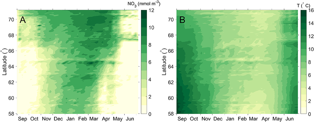
Figure 5. Simulated depth integrated (0–10 m) nitrate concentration (A) and temperature at 5 m depth (B) along the Norwegian maritime baseline (2012–2013 season). See Figure 13. The colors represent the nitrate concentration (resp. temperature) at the corresponding latitude and time along the maritime baseline.

Comparing Simulation Results With Cultivation and Survey Data

The model reproduced realistic values for the average sizes of the cultivated plants (Figure 6). The model also reproduced the ranking of the cultivation stations in terms of frond sizes. In some cases there was substantial spatial variability in the simulation results as well as in the cultivation data (cf. 1, 2, and 5 in Figure 6).

FIGURE 6

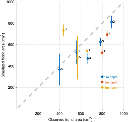
Figure 6. Simulated (ordinate axis) against observed (abscissa) S. latissima frond areas for the 5 cultivation trials in Central Norway from 2011 to 2016. The observed values are means of n = 60–200 individuals (section Cultivation trials). The ordinate values are means of the simulated frond area in 3 × 3 grid cells around the cultivation location. The vertical lines represent the range of the minimum to the maximum simulated frond area within these 3 × 3 grid cells. The numbers (1 to 5) in the plot correspond to the different cultivation locations shown in Figure 9. The colors indicate cultivation depth (2, 5, or 8 m). At stations 3, 4, and 5 more than one cultivation depth was used.

There was a clear relationship between the simulated sugar kelp frond area and the coverage of naturally occurring sugar kelp along the coast of southern Norway (Figure 7). The simulated mean frond areas increased significantly from locations with no naturally growing sugar kelp (class 0) to locations with single individuals (class 1). There was also an increase in simulated mean frond areas from locations with single individuals (class 1) to locations with a few individuals (scarce occurrences, class 2). Going from class 2 (scarce) to 3 (moderately dense kelp forest), the increase in simulated average frond areas was significant, except in 2015. There was no difference in simulated mean frond areas in locations with moderately dense kelp forest (class 3) to completely dense canopy forest (class 4). A partial comparison of simulation results with the kelp coverage data using a higher resolution model was made, without significantly different results.

FIGURE 7

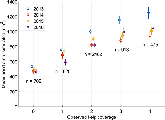
Figure 7. Comparison of simulated frond areas from four growth seasons (2013–2016) with observed sugar kelp coverage of wild populations, from field survey data. The locations for the sampling points of the field surveys are shown in Figure 4. Kelp coverage was defined semi-quantitatively as a five-step scale: 0 (absent), 1 (single individuals), 2 (scarce, i.e., a few individuals), 3 (common/moderately dense, i.e., many plants, but not a completely dense canopy cover), or 4 (dominating, i.e., a completely dense canopy cover). The five-step scale is displayed along the abscissa. Mean simulated frond areas (section Cultivation trials) for the locations in each of the five categories, for each of the four seasons, are represented by circles. The vertical line segments are 95% confidence intervals for the means of the simulated frond areas for each of the five categories. The number of observations for each kelp population density are included. The field data come from different Norwegian monitoring programs; see text for details and references.

Kelp Cultivation Potential

The Index

The index for the cultivation potential for S. latissima (1) had a tendency to increase with distance from the shore (Figure 8). In general, the best locations for cultivation were outside the six Norwegian ecoregions outlined by curves of different colors, the outer limits of which lie 1 nautical mile beyond the maritime baseline. The index was highest beyond the geographic shelf break (bottom depth > 500 m; e.g., Figure 8, 1) in Central Norway and beyond the Norwegian trench (Figure 8, 2) outside western Norway. There were large regions on the relatively wide shelf outside Central Norway with a high production potential (Figure 8, 3). Most coastal and fjord locations got lower scores. The index was similar in the Oslo fjord (Figure 8, 4) and the Porsanger fjord (Figure 8, 5) despite a latitudinal distance of 10 degrees. There were some minor discontinuities in the data along the interfaces between the model domains, but the overall picture was consistent (Figure 8).

FIGURE 8

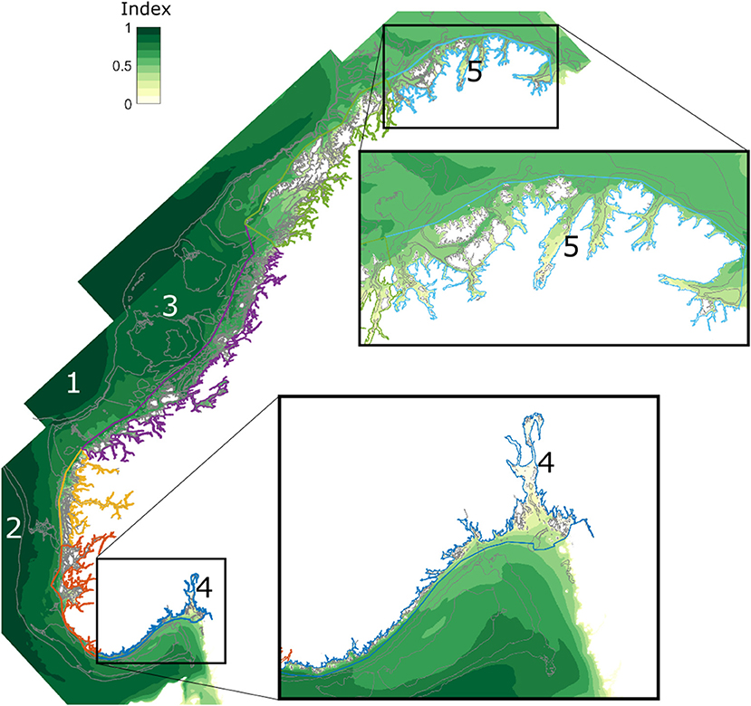
Figure 8. A spatial index for the cultivation potential of S. latissima in Norway, calculated according to (1) based on simulations using the model domains of 800 m horizontal resolution. The colored regions indicate the 6 coastal marine ecoregions in Norway: Skagerrak (dark blue), the North Sea (S) (orange), the North Sea (N) (yellow), the Norwegian Sea (S) (purple), the Norwegian Sea (N) (green), and the Barents Sea (light blue). The gray curves indicate the 200, 300, and 500 m isobaths. The extent of the map into the ocean is limited by the extent of the model domains (Figure 3). The details show the regions of Skagerrak (to the south) and the Barents Sea (to the north). The numbers refer to specific locations discussed in the text and used in Figure 11.

The index calculated for a part of the coastal region of Central Norway from the 160 m simulations revealed more details (Figure 9, which uses a different colormap than Figure 8, normalized only with respect to the maximum within the region presented there). The fjords (e.g., the Trondheim fjord, Figure 9, A) had a relatively low potential for cultivation of S. latissima, though there was some local variation, cf. the western and central parts of the Trondheim fjord. Among sheltered locations outside the fjords, station 3 seems to have good potential as well as station 2. Frohavet (B) is a large region with a relatively high potential, albeit with a bottom depth of 100–400 m and possibly large waves. The area just south of Froan (C) is more sheltered than B, with shallower bottom depth and with some of the greatest potential in the region.

FIGURE 9

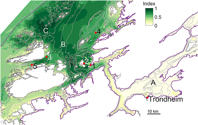
Figure 9. Spatial index for the cultivation potential of S. latissima in Central Norway, in the Norwegian Sea (S) region, calculated according to (1) based on results from model simulations of 160 m horizontal resolution (see section Model simulations). The coloring scheme used here is different from the one in Figure 8, and direct comparisons between Figure 8 and this figure do not make sense. The city of Trondheim (63.4°N ; 10.4°E) is indicated, as well as the stations 1 to 5 of the cultivation trials reported in Figure 6. The black line segment indicates the scale of the region covered. The gray curves are 100, 200, and 300 m isobaths. A, B, and C indicated the Trondheim fjord, Frohavet, and the southern end of the Froan archipelago, respectively.

Biomass Estimates

The average S. latissima cultivation potential, expressed in terms of biomass yield per unit area (3), was similar between the six ecoregions for the September deployments (Figure 10, left bars). The southern Norwegian Sea (the purple bars in Figure 10) tended toward a slightly higher biomass yield for the September deployment than the other regions (average over 4 years 20% higher than in Skagerrak), while the Barents Sea (light blue bars) had yields in the low end (average over 4 years 25% lower than in Skagerrak).

FIGURE 10

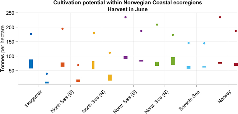
Figure 10. Spatial averages for the kelp production potential over the 6 ecoregions in Figure 8 calculated according to (3), taking into account only the grid cells with bottom depth > 50 m. The colors correspond to the colors outlining the regions in Figure 8. The bars span from minimum to maximum spatial means over the cultivation seasons 2012–2015. The filled-in dots are the average maxima, over all seasons, for each region. The left bars and dots for each region indicate deployment in September, whereas the right ones represent deployment in February the following year). Harvest in the beginning of June is assumed.

For the February deployments (the rightmost bars for each region, Figure 10), the yields were generally lower than for the September deployments, except for the northern Norwegian Sea (green bars). In particular in the three southernmost regions (Skagerrak, North Sea S and N) the yields from the February deployments were significantly lower than from the September deployments, also in a statistical sense. Averaging over the Norwegian coast as a whole, there was little difference between deploying in autumn and in late winter. Deployment in September yielded similar averaged and maximum values throughout all the regions, though with a peak in the Norwegian Sea regions.

Within each of the regions there was a significant interannual variation in the cultivation potential for S. latissima, expressed by the vertical extent of the bars (Figure 10). The spatial variation in the production potential was also significant, as indicated by the positions of the circles relative to the vertical bars in Figure 10, in particular in Skagerrak and the northern part of the Norwegian Sea. For the country as a whole, the interannual variation was not great.

Outside the maritime baseline (locations 1 to 3 in Figure 8) the cultivation potential was typically comparable to the maximum for the inside of the line, with the highest potential yields off the shelf break (Figure 11).

FIGURE 11

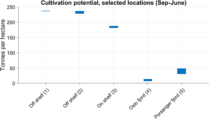
Figure 11. The cultivation potential of S. latissima, calculated according to (2), at the locations labeled 1 to 5 in Figure 8. The vertical range of the bars indicate the minimum to the maximum production over the seasons 2012–2015.

Time and Latitude

There were differences in the average (geometric mean) seasonal growth pattern between the southern and northern ecoregions (Figure 12). While growth initiated later in the Barents Sea than in the Skagerrak, the harvestable size of the plants in the beginning of June was similar. When deployed in September, kelp growth in the south (Skagerrak) continued through autumn, winter and spring (Figure 12, continuous blue curve), while in the north (Norwegian Sea, S) there was no net growth between early December and late January (continuous red curve). In the far north (Barents Sea) the average frond size even declined slightly from late November until early February (continuous yellow curve). For the February deployment the growth in the Barents Sea caught up with that in Skagerrak quite early. The simulated frond sizes of the plants from the February “deployment” in the Barents Sea surpassed those of the Skagerrak plants by about an order of magnitude by early June. The variation in frond sizes between different locations in the Skagerrak region was greater than in the other two regions, throughout the entire growth period and for both deployment times studied, as seen from the (geometric) standard deviations (Figure 12, shaded regions).

FIGURE 12

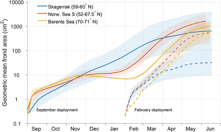
Figure 12. Time series for average (spatial geometric mean) simulated frond areas within the Skagerrak (blue lines), Norwegian Sea S (red lines), and Barents Sea (yellow lines) ecoregions (see Figure 8) at 1.5 m depth. The continuous lines represent deployments in September, while the dashed lines represent deployments in February. The shaded regions indicate the geometric standard deviation factors within each region. Note the logarithmic scale of the ordinate axis.

While the period of the maximal biomass specific growth rate (excluding the very first period after deployment) was February-March, the absolute daily biomass growth was highest from the end of April into July (Figure 13). There was a clear trend in the timing of the maximal daily (dry) biomass growth along the outer boundary of the ecoregions for the September deployments. There was up to 2 months between the timing of the maximal daily growth rate from the southernmost and northernmost points along the coast at 58 ° and 71 °N, respectively, both for absolute and specific daily growth rates. Recall that if B_n and B_n+1 denote the biomass on 2 consecutive days, then the specific and absolute daily growth rates are calculated as ln(B_n+1) - ln(B_n) and B_n+1- B_n, respectively.

FIGURE 13

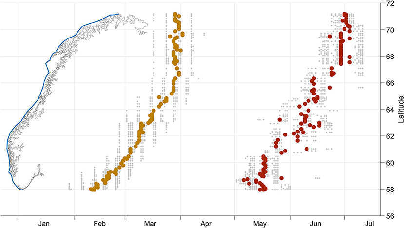
Figure 13. The effect of latitude on the timing of biomass development of S. latissima deployed in September. The simulated DW of individuals was sampled along the baseline (blue line along the Norwegian coastline) from the 2013–2015 simulations. The yellow dots indicate the average time (abscissa axis) of the highest daily specific growth rates plotted against latitude (ordinate axis on the right) over the three seasons. The red dots indicate the average time of the highest absolute daily growth rate against latitude over the three seasons. The small gray dots indicate the data used to compute the averages.

Discussion

This paper highlights important aspects of the cultivation potential for the kelp species S. latissima in Norway such as location (fjord, nearshore, offshore) and latitude. How the key environmental variables for growth vary and interact in time and space and how these affect the timing of deployment and the cultivation cycle are also considered. The evaluation of the results against cultivation data and field survey data on the density of natural populations of S. latissima support the results, but there is yet no empirical data on the offshore kelp cultivation potential.

Model Evaluation and Uncertainty

The evaluation exercise performed here (section The environmental variables simulated by SINMOD) is important for at least two reasons. Firstly, because it shows that the dynamical model (SINMOD) provides realistic values for sizes of plants and is able to reproduce spatial differences between locations (e.g., 1 and 2 in Figure 6). Secondly, because the simulated production potential is related to suitability of locations for growth of natural kelp populations. This indicates a potential for the model to identify actual locations suitable for kelp cultivation. The simulation results further indicate a potential for kelp cultivation in many regions in which naturally growing S. latissima is absent (Figure 7). This is because the model simulates the suitability of areas for kelp production in the water masses as a function of the prevailing physical and chemical conditions, regardless of the suitability of the seabed for growth of natural kelps and their possibilities of completing a full life cycle. The model was not tuned to any of the data used in the present paper. Previous partial validations have been provided in Broch et al. (2013) and Fossberg et al. (2018).

Some North Atlantic kelp species have been found to have a clear response to (changes in) day length (Lüning, 1993; Rinde and Sjøtun, 2005; Krause-Jensen et al., 2016), but the exact “functional response” of S. latissima to these environmental signals is not known. It is difficult to formulate realistic mathematical growth models without taking the photoperiod into account in some way or another, in particular at relatively high latitudes (Broch and Slagstad, 2012).

The key environmental variables limiting macroalgal growth have been considered here. These are nutrients, light, temperature, and ocean currents (Wiencke and Bischof, 2012), but there are also a number of variables that have not been taken into account. It has been assumed here that nitrogen is the main (macro) nutrient limiting growth (Hurd et al., 2014). Phosphorous may also be of importance in certain cases. Micronutrients and trace elements have not been considered, nor has the concentration of CO₂. Epiphyte infestation is of great importance for macroalgae aquaculture, as well as exposure and wave height (van der Molen et al., 2018).

In the present simulations the same set of numerical values for the kelp growth parameters were used (Broch and Slagstad, 2012; Broch et al., 2013; Fossberg et al., 2018) for the entire Norwegian coast. Further data on responses of ecotypes will provide a better basis for modeling and thus the understanding the true role of changes in environmental conditions for the growth of S. latissima.

Index, Biomass Estimates, and Production Potential

The main result from the spatial index estimates is that the potential seemed to be higher offshore than nearshore. There are several explanations for this. Firstly, in fjords and in the Norwegian Coastal Current (NCC) the surface waters have lower salinity, which may have an adversary effect on growth and production in S. latissima (Mortensen, 2017). Secondly, the nearshore stratification generally leads to an earlier phytoplankton spring bloom, with ensuing earlier nutrient depletion of the surface waters (Figure 5A) and a shorter period of nutrient uptake than further offshore. Thirdly, the coastal and nearshore waters have a higher light attenuation than oceanic waters, which means that cultivation must take place closer to the surface. As CDOM and silts were not explicitly included in the calculations of the light attenuation, the light attenuation may have been under estimated in nearshore regions, to the effect that differences in the index between near- and offshore regions might have been greater. Finally, the temperatures in the coastal waters are generally lower in winter (potentially limiting growth) and higher in summer (potentially harmful) than in oceanic waters.

Despite the production potential being higher offshore than nearshore, there were regions of locally higher production potential along the coast. This was also the case for relatively sheltered regions as seen from the 160 m model simulations. These are regions that usually have high vertical mixing, typically tidal mixing and upwelling events, providing nutrients from deeper waters also after the spring bloom period.

The index introduced here has similarities to the suitability index for S. latissima cultivation developed by van der Molen et al. (2018). The difference is that our index uses results from a kelp growth model rather than just the environmental data provided by the ecosystem model directly, and that it is based on higher spatial model resolution (800/160 m vs. 5.5 km). This means that temporal interactions between internal (nitrogen and carbon) reserves were taken into account and integrated over time and over the entire model domain.

The biomass estimates are based on upscaling (2) and must therefore be considered over estimates. However, this is not necessarily the case for the upper limits for the production potential. The relative differences in the production potentials remain valid despite the uncertainties in upscaling. Biomass production estimates from other sources are presented in Table 1. The figures have in most cases been transformed by the present authors to the common unit “t (wet weight) ha⁻¹.” Our biomass estimates have been based on averages over very large regions (~1,000 to ~10,000 km²), with substantial spatial variation within each of these. The results in Table 1 indicate that cultivation yields may vary by an order of magnitude even within a fairly small region (Bruhn et al., 2016). This emphasizes that local considerations are important when siting a farm (see section Future prospects and management below).

TABLE 1

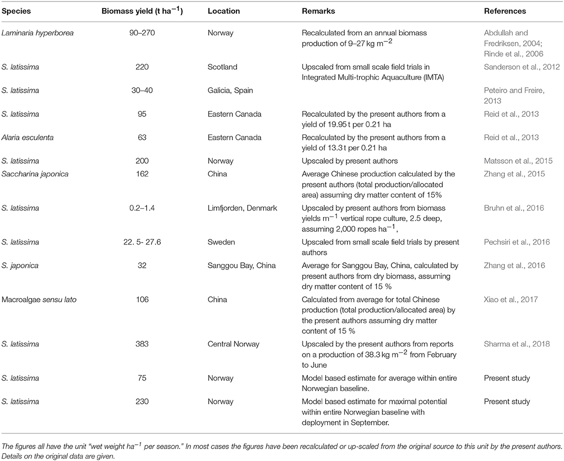
Table 1. Some previously published estimates for the kelp cultivation potential in different regions.

The results indicate that the production potential for the February deployments increased moving northward among the six marine ecoregions. This does not mean that (pelagic) primary production in general increases with latitude. Rather, this finding reflects the earlier onset of the phytoplankton spring bloom in the south. This leads to an earlier depletion of the nutrients in the surface layer and thus a shorter time-period of high nutrient concentrations available for cultivated macroalgae in the south than in the north, in particular with harvest in early June. The results on the production potential simulated for September seem to be more consistent between the ecoregions along the coast.

Along the same line, there seems to be a clear trend toward a later development moving northwards (Figures 12, 13). This is due to the combined effects of temperature, total light availability, photoperiod and nutrient availability. S. latissima production in the northern regions in some places seems to “catch up” with that in the southern regions. Thus, there is a potential for the macroalgae aquaculture industry to provide biomass at stable volumes for an extended time period. These results further underscore the importance of distinguishing between specific and absolute growth. The latter is probably most important for farming purposes.

The seasonal and geographic patterns in growth development mirrored the environmental variables like nutrient concentrations and temperature to some extent. The numerical values of the nutrient concentrations and the qualitative features of their seasonal development match those of observations (Sætre, 2007). The seasonal pattern of surface nutrient concentrations is to a great extent governed by the phytoplankton bloom dynamics, which follows a latitudinal gradient (Vikebø et al., 2012). Since the values used in Figure 5A were extracted along the maritime baseline, some sample points were further offshore than others, explaining some of the variability in the results.

We have assumed here a fixed harvest time in the beginning of June for consistency. This is later than what is common in commercial kelp farms mainly due to the onset of epiphyte infestations in late spring/early summer (Førde et al., 2016). Harvest time in the north may have been assumed to take place earlier than necessary and prolonging the growth season would increase the production potential in the north. The harvest date may impact on the composition of the biomass, with implications for its relevance for various end products (Sharma et al., 2018).

The greatest potential for S. latissima production seems to lie in relatively exposed regions and in oceanic waters outside the coastal zones. We have not considered the existence of suitable technology for macroalgae cultivation in such environments, but there have been successful cultivation trials and some technological development in this direction (Buck and Buchholz, 2005; Buck et al., 2017; Bak et al., 2018). However, deploying and harvesting kelp cultures far offshore will increase transport and energy costs, which might outweigh the benefits of increased biomass (Burg et al., 2017).

Many of the considerations presented here probably remain valid for other kelp species, like Laminaria digitata and Alaria esculenta. Different tolerance levels for, e.g., low salinity points toward a potential for using, e.g., L. digitata in fjord environments where it may have an advantage over S. latissima (Kerrison et al., 2015; Mortensen, 2017).

Environmental Effects and Interactions

There are most likely both positive and negative impacts of macroalgae cultivation on coastal environments. Examples of potentially positive effects are that cultivation of macroalgae may mitigate effects of ocean acidification (Duarte et al., 2017; Krause-Jensen et al., 2018) and eutrophication (Xiao et al., 2017). Examples of negative effects are reduced oxygen levels due to loss and degradation of organic matter or nutrient depletion in oligotrophic areas. At the moment European kelp farms are relatively small, with a total production of < 1,000 tons a year (FAO, 2016), and at such a level large scale negative effects seem unlikely. Some studies on the bene—fits and effects of macroalgal cultivation both from China (Zhang et al., 2009; Xiao et al., 2017) and Europe (Walls et al., 2017; Hasselström et al., 2018) have been made.

Here, the focus has been on mapping the potential for biomass production. Evaluation of different production regions may also be performed with a view to, e.g., minimize environmental effects (nutrient depletion, organic enrichment by dislodges plants and eroded tissue) or interactions between kelp farms and other types of aquaculture (spread of diseases and parasites between farms etc.). We have not considered Integrated Multi-Trophic Aquaculture (IMTA) in this study, though this is a practice that may increase biomass yields locally (Broch et al., 2013; Handå et al., 2013; Fossberg et al., 2018; Jansen et al., 2018) and may be particularly attractive in regions where space is limiting development of aquaculture.

In reality, a large kelp farm may experience a reduction in the transport of nutrients within the farm due to nutrient uptake by the kelp, or the plants may experience light shading due to the se—eding density (Broch et al., 2013). It has not been possible to address these aspects here, as a two-way feedback between the kelp and ecosystem module in the present simulations would result in substantial nutrient uptake everywhere, and hence would prevent an assessment of the baseline conditions for the cultivation potential.

Future Prospects and Management

By January 2017 there were a total of 309 permits for macroalgae cultivation in Norway, of which roughly half were awarded for kelp cultivation (S. latissima, L. digitata, A. esculenta) (Norwegian Directorate of Fisheries, 2018), with S. latissima at present being the commercially most important species. The total kelp production for 2017 amounted to 145 tons with a sales value of approximately 74,000 Euro (Ibid.). It has been suggested that by 2050 the Norwegian aquaculture industry could produce 20 million tons of kelp with a turnover of 4 billion Euro annually (Olafsen et al., 2012). According to the average production potential for the entire Norwegian coast in Figure 10 this would require an area in the range of 2,700–3,000 km². By comparison the sea area inside the Norwegian maritime baseline covers 89,091 km², excluding Svalbard and Jan Mayen. Such figures are deceptively large as there are a multitude of interests competing for space in the coastal zone, illustrated by van der Molen et al. (2018). Thus, careful planning is required for successful siting of macroalgae cultivation facilities and to optimize value chains from deployment of seedlings, through harvest and processing, to the end market of the products based on the biomass. GIS-type analyses will be necessary, and the present results provide a basis for this. Future constraints may include minimizing environmental impacts and sources of pollution. Future possibilities lie in moving from the coastal region into the ocean.

Author Contributions

OB, MA, TB, HG, SF, AH, JS, and KH all conceived and planned the article. OB and MA performed the coupled model simulations. SF, JS, and AH executed the kelp cultivation trials and sampling. TB and HG contributed to the natural kelp field surveys. All authors contributed to the analysis of the results and the writing of the paper.

Funding

The research reported in this paper was mainly supported by the Research Council of Norway grants 267536 (KELPPRO) and 254883 (MACROSEA) and by the county authorities of Møre-and-Romsdal and Trøndelag. HPC resources were made available through NOTUR grant no. NN2967k. Two of the cultivation trials were executed in the Research Council of Norway project 244244 (PROMAC).

Conflict of Interest Statement

The authors declare that the research was conducted in the absence of any commercial or financial relationships that could be construed as a potential conflict of interest.

References

Abdullah, M. I., and Fredriksen, S. (2004). Production, respiration and exudation of dissolved organic matter by the kelp Laminaria hyperborea along the west coast of Norway. J. Mar. Biol. 84, 887–894. doi: 10.1017/S002531540401015Xh

CrossRef Full Text | Google Scholar

Bak, U. G., Mols-Mortensen, A., and Gregersen, O. (2018). Production method and cost of commercial-scale offshore cultivation of kelp in the Faroe Islands using multiple partial harvesting. Algal Res. 33, 36–47. doi: 10.1016/j.algal.2018.05.001

CrossRef Full Text | Google Scholar

Bartsch, I., Wiencke, C., Bischof, K., Buchholz, C. M., Buck, B. M., Eggert, A., et al. (2008). The genus Laminaria sensu lato: recent insights and developments. Eur. J. Phycol. 43, 1–86. doi: 10.1080/09670260701711376

CrossRef Full Text | Google Scholar

Bekkby, T., Moy, F. E., Olsen, H., Rinde, E., Bodvin, T., Bøe, R., et al. (2013). “The Norwegian program for mapping of marine habitats – providing knowledge and maps for ICZMP,” in Global Challenges in Integrated Coastal Zone Management, Vol II, eds E. Moksness, E. Dahl, and J. Støttrup (Oxford: John Wiley and Sons), 21–30.

Google Scholar

Beldring, S., Engeland, K., Roald, L. A., Sælthun, N. R., and Voksø, A. (2003). Estimation of parameters in a distributed precipitation-runoff model for Norway. Hydrol Earth System Sci. 7, 304–316. doi: 10.5194/hess-7-304-2003

CrossRef Full Text | Google Scholar

Bolton, J. J., and Lüning, K. (1982). Optimal growth and maximal survival temperatures of atlantic laminaria species (Phaeophyta) in culture. Mar. Biol. 66, 89–94. doi: 10.1007/BF00397259

CrossRef Full Text | Google Scholar

Broch, O. J., Ellingsen, I. H., Forbord, S., Wang, X., Volent, Z., Alver, M. O., et al. (2013). Modelling the cultivation and bioremediation potential of the kelp Saccharina Latissima in close proximity to an exposed salmon farm in Norway. Aquacult. Environ. Interact. 4, 187–206. doi: 10.3354/aei00080

CrossRef Full Text | Google Scholar

Broch, O. J., and Slagstad, D. (2012). Modelling seasonal growth and composition of the kelp Saccharina latissima. J Appl. Phycol. 24, 759–776. doi: 10.1007/s10811-011-9695-y

CrossRef Full Text | Google Scholar

Bruhn, A., Tørring, D. B., Thomsen, M., Canal-Vergés, P., Nielsen, M. M., Rasmussen, M. B., et al. (2016). Impact of environmental conditions on biomass yield, quality, and bio-mitigation capacity of Saccharina latissima. Aquacult. Environ. Interact. 8, 619–636. doi: 10.3354/aei00200

CrossRef Full Text | Google Scholar

Buck, B. H., and Buchholz, C. M. (2005). Response of offshore cultivated Laminaria saccharina to hydrodynamic forcing in the North Sea. Aquaculture 250, 674–691. doi: 10.1016/j.aquaculture.2005.04.062

CrossRef Full Text | Google Scholar

Buck, B. H., Nevejan, N., Wille, M., Chambers, M. D., and Chopin, T. (2017). “Offshore and multi-use aquaculture with extracte species: seaweeds and bivalves,” in Aquaculture Perspective of Multi-Use Sites in the Open Ocean, eds B. H. Buck and R. Langan (Cham: Springer International Publishing AG), 23–69.

Google Scholar

Burg, S. W. K., Duijn, A. P., Bartelings, H., Krimpen, M. M., and Poelman, M. (2017). The economic feasibility of seaweed production in the North Sea. Aquacult. Econ. Manage. 20, 235–252. doi: 10.1080/13657305.2016.1177859

CrossRef Full Text | Google Scholar

Dale, T., Fagerli, C. W., Trannu, H., Eikrem, W., Staalstrøm, A., and Kristiansen, T. (2018). ØKOKYST Delprogram Nordsjøen Nord, Annual report 2017, Årsrapport 2017. Miljødirektoratet rapport M-1009. (Annual report 2017, Norwegian Environment Agency, M-1009)

Dee, D. P., Uppala, S. M., Simmons, A. J., Berrisford, P., Poli, P., Kobayashi, S., et al. (2011). The ERA-interim reanalysis: configuration and performance of the data assimilation system. Q. J. Royal Meteorol. Soc. 137, 553–97. doi: 10.1002/qj.828

CrossRef Full Text | Google Scholar

Direktoratsgruppen vanndirektivet (2018). Veileder 2:2018 Klassifisiering av miljøtilstand i vann (The Directorate group for implementation of the water directive, Norway). Norwegian Environment Agency. Available online at: www.vannportalen.no

Duarte, C. M., Wu, J., Xiao, X., Bruhn, A., and Krause-Jensen, D. (2017). Can seaweed farming play a role in climate change mitigation and adaptation? Front. Mar. Sci. 4:100. doi: 10.3389/fmars.2017.00100

CrossRef Full Text | Google Scholar

Fagerli, C. W., Staalstrøm, A., Trannum, H. C., Gitmark, J. K., Eikrem, W., Marty, S., et al. (2018). ØKOKYST Delprogram Nordsjøen Nord, Årsrapport 2017. Miljødirektoratet rapport M-1007. Annual report 2017, Norwegian Environment Agency, M-1007.

FAO (2016). The State of World Fisheries and Aquaculture 2016. Contributing to Food Security and Nutrition for All. Rome.

FAO (2018). The Global Status of Seaweed Production, Trade and Utilization. Globefish Research Programme Volume 124. Rome.

Foldal, S. (2018). Morphological relations of cultivated Saccharina latissima at three stations along the Norwegian coast (In Norwegian). Master's thesis in Marine Coastal Development, Norwegian University of Science and Technology.

Forbord, S., Steinhovden, K. B., Rød, K. K., Handå, A., and Skjermo, J. (2018). “Cultivation protocol for Saccharina latissima,” in Protocols for Macroalgae Research, 1st Edn., eds B. Charrier, T. Wichard, and C. R. K. Reddy (Boca Raton, FL; London; New York, NY: CRC Press), 37–59.

Google Scholar

Førde, H., Forbord, S., Handå, A., Fossberg, J., Arff, J., Johnsen, G., et al. (2016). Development of bryozoan fouling on cultivated kelp (Saccharina latissima) in Norway. J. Appl. Phycol. 28, 1225–1234. doi: 10.1007/s10811-015-0606-5

CrossRef Full Text | Google Scholar

Fossberg, J., Forbord, S., Broch, O. J., Malzahn, A. M., Jansen, H., Handå, A., et al. (2018). The potential for upscaling kelp (Saccharina latissima) cultivation in salmon-driven integrated multi-trophic aquaculture (IMTA). Front. Mar. Sci. 5:418. doi: 10.3389/fmars.2018.00418

CrossRef Full Text | Google Scholar

Gundersen, H., Bekkby, T., Christie, H., Moy, F. E., and Tveiten, L. A. (2012). Development of an Indicator for Sugar Kelp (Saccharina latissima) for the Norwegian Nature Index - Modeling Reference Condition for Area Distribution. NIVA Report No. 6438-2012 (In Norwegian).

Handå, A. H., Forbord, S., Wang, X., Broch, O. J., Dahle, S. W., Størseth, T. R., et al. (2013). Seasonal- and depth-dependent growth of cultivated kelp (Saccharina latissima) in close proximity to salmon (Salmo salar) aquaculture in Norway. Aquaculture 414-415, 191–201. doi: 10.1016/j.aquaculture.2013.08.006

CrossRef Full Text | Google Scholar

Harsson, B. G., and Preiss, G. (2012). Norwegian baselines, Maritime boundaries and the UN convention on the law of the sea. Arct. Rev. Law Polit. 3, 108–129.

Google Scholar

Hasselström, L., Wisch, W., Gröndahl, F., Nylund, G. M., and Pavia, H. (2018). The impact of seaweed cultivation on ecosystem services - a case study from the west coast of Sweden. Mar. Pol. Bul. 133, 53–64. doi: 10.1016/j.marpolbul.2018.05.005

PubMed Abstract | CrossRef Full Text | Google Scholar

Hersoug, B. (2013). “The battle for space - the position of Norwegian aquaculture in integrated Coastal Zone planning,” in Global Challenges in Integrated Coastal Zone Management, eds E. Moksness, E. Dahl, and J. Støttrup (Hoboken, NJ: Wiley-Blackwell), 159–168. doi: 10.1002/9781118496480.ch12

CrossRef Full Text | Google Scholar

Holdt, S. L., and Kraan, S. (2011). Bioactive compounds in seaweed: function food applications and legislation. J. Appl. Phycol. 23, 643–697. doi: 10.1007/s10811-010-9632-5

CrossRef Full Text | Google Scholar

Hurd, C. L., Harrison, P. J., and Druehl, L. D. (1996). Effect of seawater velocity on inorganic nitrogen uptake by morphologically distinct forms of Macrocystis integrifolia from wave-sheltered and exposed sites. Mar. Biol. 126, 205–214. doi: 10.1007/BF00347445

CrossRef Full Text | Google Scholar

Hurd, C. L., Harrison, P. J., Bischof, K., and Lobban, C. S. (2014). Seaweed ecology and physiology. Cambridge: Cambridge University Press.

Google Scholar

Jansen, H., Broch, O. J., Bannister, R., Cranford, P., Handå, A., Husa, V., et al. (2018). Spatio-temporal dynamics in the dissolved nutrient waste plume from Norwegian salmon cage aquaculture. Aquacult. Environ. Interact. 10, 385–399. doi: 10.3354/aei00276

CrossRef Full Text | Google Scholar

Kerrison, P., Stanley, M. S., Edwards, M. D., Black, K. D., and Hughes, A. D. (2015). The cultivation of European kelp for bioenergy: site and species selection. Biomass Bioenergy 80, 229–242. doi: 10.1016/j.biombioe.2015.04.035

CrossRef Full Text | Google Scholar

Kraan, S. (2016). “Seaweed and alcohol: biofuel or booze?,” in Seaweed in Health and Disease Prevention, eds J. Fleurence and I. Levine (Cambridge, MA: Academic Press), 169–184.

Google Scholar

Krause-Jensen, D., Lavery, P., Serrano, O., Marbà, N., Masque, P., and Duarte, C. M. (2018). Sequestration of macroalgal carbon: the elephant in the Blue Carbon Room. Biol. Lett. 14:20180236. doi: 10.1098/rsbl.2018.0236

PubMed Abstract | CrossRef Full Text | Google Scholar

Krause-Jensen, D., Marbà, N., Sanz-Martin, M., Hendriks, I. E., Thyrring, J., Carstensen, J., et al. (2016). Long photoperiods sustain high pH in Arctic kelp forests. Sci. Adv. 2:e1501938. doi: 10.1126/sciadv.1501938

PubMed Abstract | CrossRef Full Text | Google Scholar

Lehahn, Y., Ingle, K. N., and Golberg, A. (2016). Global potential of offshore and shallow waters macroalgal biorefineries to provide for food, chemicals and energy: feasibility and sustainability. Algal Res. 17, 150–160. doi: 10.1016/j.algal.2016.03.031

CrossRef Full Text | Google Scholar

Lüning, K. (1993). Environmental and internal control of seasonal growth in seaweeds. Hydrobiologia 260/261, 1–14. doi: 10.1007/978-94-011-1998-6_1

CrossRef Full Text | Google Scholar

Matsson, S., Mogård, S., Fieler, R., Christie, H., and Neves, L. (2015). Pilot Study of Kelp Cultivation in Troms, Norway. Report, Akvaplan-niva (Tromsø), Norwegian.

Google Scholar

Mortensen, L. (2017). Diurnal carbon dioxide exchange rates of Saccharina latissima and Laminaria digitata as affected by salinity levels in Norwegian Fjords. J. Appl. Phycol. 29:3067. doi: 10.1007/s10811-017-1183-6

CrossRef Full Text | Google Scholar

Moy, F., Christie, H., Steen, H., Stålnacke, P., Aksnes, D., Alve, E., et al. (2009). Sluttrapport fra Sukkertareprosjektet 2005-2008. SFT-rapport 2467. (Norwegian Environment Agency).

Norwegian Directorate of Fisheries (2018). Aquaculture Statistics for Algae. Available online at: https://www.fiskeridir.no/Akvakultur/Statistikk-akvakultur/Akvakulturstatistikk-tidsserier/Alger (Accessed October 4, 2018).

Olafsen, T., Winther, U., Olsen, Y., and Skjermo, J. (2012). Value Creation Based on Productive Seas in 2050. (In Norwegian: Verdiskapning basert på produktive hav i 2050), Det Kongelige Norske Videnskabers Selskab (DKNVS) and Norges Tekniske Vitenskapsakademi (NTVA).

Olsen, Y. (2011). Resources for fish feed in future mariculture. Aquacult. Environ. Interact. 1, 187–200. doi: 10.3354/aei00019

CrossRef Full Text | Google Scholar

Pechsiri, J. S., Thomas, J.-B. E., Risen, E., Ribeiro, M. S., Malmstrøm, M. E., Nylund, G. M., et al. (2016). Energy performance and greenhouse gas emissions of kelp cultivation for biogas and fertilizer recovery in Sweden. Sci. Tot. Env. 573, 347–355. doi: 10.1016/j.scitotenv.2016.07.220

PubMed Abstract | CrossRef Full Text | Google Scholar

Peteiro, C., and Freire, O. (2013). Biomass yield and morphological features of the seaweed Saccharina latissima cultivated at two different sites in a coastal bay in the Atlantic coast of Spain. J. Appl. Phycol. 25, 205–213. doi: 10.1007/s10811-012-9854-9

CrossRef Full Text | Google Scholar

Reid, G. K., Chopin, T., Robinson, S. M. C., Azevedo, P., Quinton, M., and Belyea, E. (2013). Weight ratios of the kelps, Alaria esculenta and Saccharina latissima, required to sequester dissolved inorganic nutrients. and supply oxygen for Atlantic salmon, Salmo salar, in Integrated Multi-Trophic Aquaculture systems. Aquaculture 408-409, 34–46. doi: 10.1016/j.aquaculture.2013.05.004

CrossRef Full Text | Google Scholar

Rinde, E., Christie, H., Bekkby, T., and Bakkestuen, V. (2006). Ecological Effects of Kelp Trawling. (In Norwegian: Økologiske Effekter av Taretråling. Analyser basert på GIS-modellering og empiriske data). NIVA report no LNR 5150–200.

Rinde, E., and Sjøtun, K. (2005). Demographic variation in the kelp Laminaria hyperborea along a latitudinal gradient. Mar. Biol. 146, 1051–1062. doi: 10.1007/s00227-004-1513-5

CrossRef Full Text | Google Scholar

Sætre, R. (ed.). (2007). The Norwegian Coastal Current. Trondheim: Tapir Academic Press.

Google Scholar

Sanderson, J. C., Dring, M. J., Davidson, K., and Kelly, M. S. (2012). Culture, yield and bioremediation potential ofPalmaria palmata (Linnaeus) Wber and Mohr and Saccharina latissima (Linnaeus) C. E Lane, C. Mayes, Druehl, and G. W. Saunders adjacent to fish farm cages in NorthWest Scotland. Aquaculture 354-355, 128–135. doi: 10.1016/j.aquaculture.2012.03.019

CrossRef Full Text | Google Scholar

Sharma, S., Neves, L., Funderud, J., Mydland, L. T., Øverland, M., and Horn, S. J. (2018). Seasonal and depth variations in the chemical composition of cultivated Saccharina latissima. Alg. Res. 32, 107–112. doi: 10.1016/j.algal.2018.03.012

CrossRef Full Text | Google Scholar

Slagstad, D., and McClimans, T. A. (2005). Modeling the ecosystem dynamics of the barents sea including the marginal ice zone: I. Physical and chemical oceanography. J. Mar. Syst. 58, 1–18. doi: 10.1016/j.jmarsys.2005.05.005

CrossRef Full Text | Google Scholar

van der Molen, J., Ruardij, P., Mooney, K., Kerrison, P., O'Connor, N. E., Gorman, E., et al. (2018). Modelling potential production of macroalgae farms in UK and Dutch coastal waters. Biogeosciences 16, 1123–1147. doi: 10.5194/bg-15-1123-2018

CrossRef Full Text | Google Scholar

Vikebø, F., Korosov, A., Stenevik, E. K., Husebø, Å., and Slotte, A. (2012). Spatio-temporal overlap of hatching in Norwegian spring-spawning herring and the spring phytoplankton bloom at available spawning substrata. ICES J. Mar. Sci. 69, 1298–1302. doi: 10.1093/icesjms/fss083

CrossRef Full Text | Google Scholar

Walls, A. M., Kennedy, R., Edwards, M. D., and Johnson, M. P. (2017). Impact of kelp cultivation on the ecological status of benthic habitats and Zostera marina seagrass biomass. Mar. Poll. Bull.123, 19–27. doi: 10.1016/j.marpolbul.2017.07.048

PubMed Abstract | CrossRef Full Text | Google Scholar

Wassmann, P., Slagstad, D., Riser, C. W., and Reigstad, M. (2006). Modelling the ecosystem dynamics of the barents sea including the marginal ice zone: II. Carbon flux and interannual variability. J. Mar. Syst. 59, 1–24. doi: 10.1016/j.jmarsys.2005.05.006

CrossRef Full Text | Google Scholar

Wiencke, C., and Bischof, K. (2012). Seaweed Biology - Novel Insights Into Ecophysiology, Ecology and Utilization. Ecological Studies 2019. Heidelberg: Springer.

Google Scholar

Xiao, X., Agusti, S., Lin, F., Li, K., Pan, Y., Yu, Y., et al. (2017). Nutrient removal from Chinese coastal waters by large-scale seaweed aquaculture. Sci. Rep. 7:46613. doi: 10.1038/srep46613

PubMed Abstract | CrossRef Full Text | Google Scholar

Zhang, J., Hansen, P. K., Fang, J., Wang, W., and Jiang, Z. (2009). Assessment of the local environmental impact of intensive marine shellfish and seaweed farming - application of the MOM system in the Sungo Bay, China. Aquaculture 287, 304–310. doi: 10.1016/j.aquaculture.2008.10.008

CrossRef Full Text | Google Scholar

Zhang, J., Wu, W., Ren, J. S., and Lin, F. (2016). A model for the growth of mariculture kelp Saccharina japonica in Sanggou Bay, China. Aquacult. Environ. Interact. 8, 273–283. doi: 10.3354/aei00171

CrossRef Full Text | Google Scholar

Zhang, N., Zhang, Y., Tao, L., Guo, J., Sun, X., Li, N., et al. (2015). Construction of a high density snp linkage of kelp (Saccharina japonica) by sequencing Taq I site associated DNA and mapping of a sex determining locus. BMC Genomics 16:189. doi: 10.1186/s12864-015-1371-1

PubMed Abstract | CrossRef Full Text | Google Scholar