Marine CO2 Patterns in the Northern Salish Sea

Introduction

The marine carbon dioxide (CO₂) system in coastal settings is influenced by a host of processes that are unique to the land-ocean boundary (e.g., freshwater inputs, coastal upwelling and downwelling circulations, benthic-pelagic coupling, eutrophication, and the uptake of anthropogenic CO₂) and create a complicated mosaic of spatially and temporally varying seawater CO₂ conditions (Feely et al., 2016; Chan et al., 2017) that hinders long-term trend detection in the absence of lengthy observational records (Sutton et al., 2018). Resolving the downward trajectories of seawater pH and carbonate ion (${\mathrm{CO}}_3^{2-}$) concentration that result from the uptake of anthropogenic CO₂, termed ocean acidification (OA; Caldeira and Wickett, 2003; Feely et al., 2004; Orr et al., 2005), is of specific interest because of the anticipated impacts on marine ecosystems and the services they provide (Cooley et al., 2009; Doney et al., 2012), as well as downstream economic consequences by jeopardizing food security and fisheries revenue, and destabilizing coastal communities (Cooley and Doney, 2009; Ekstrom et al., 2015; Mathis et al., 2015; Seung et al., 2015). Understanding secular change in CO₂ system parameters associated with OA is critical in order to forecast the ecological implications, however, the effort is significantly impaired in coastal settings that contain sparse CO₂ system information in the context of large inherent dynamic variability.

The Salish Sea is one of the largest inland seas on the North American Pacific Coast, is bi-national with a shared border between the United States of America (Washington State) and Canada (British Columbia, BC), and consists of a collection of straits, sounds, and inlets; the largest waterways being: Strait of Juan de Fuca, Puget Sound, and the Strait of Georgia. The Northern Salish Sea (NSS) is defined here as the Strait of Georgia and peripheral waterways north of Lasqueti Island and south of Quadra Island (Figure 1). The along-axis of the NSS is oriented ∼50° west of true north, and the distance spanned along this axis is ∼110 km. The NSS cross-axis is narrower and spans ∼50 km at its widest point (near Baynes Sound; Figure 1). The maximum depth of the NSS is ∼350 m and deep water exchange with the open shelf is thought to mainly occur via a flow pathway over ∼100 m sills in the southern Strait of Georgia (Masson, 2002; Johannessen et al., 2014). Deep water renewal occurs annually during summer and maximal surface water residence times are at most a few months (Masson, 2002; Pawlowicz et al., 2007). The NSS is bounded by coastal mountains on both Vancouver Island and mainland BC, such that wind patterns are highly channelized (i.e., oriented along channel; Figure 1) with predominantly northwesterly winds in summer and southeasterly winds in winter (Bakri et al., 2017). The Fraser River is the dominant freshwater source to the southern Salish Sea, with peak discharge near 10,000 m³ s^-1 during the summer snow/ice melt freshet (Masson and Cummins, 2004). Fraser River water flow-weighted mean total alkalinity (TA) is ∼700 μmol kg^-1, with higher values during lower flow states (Voss et al., 2014). Numerous smaller river systems also likely play an important role, particularly in the NSS, that collectively stratify the upper water column and allow for high spring and summer phytoplankton biomass accumulation and rates of primary production (Masson and Peña, 2009). The NSS also houses the majority of the shellfish aquaculture industry lease sites in BC (Haigh et al., 2015), and serves as an important region for migrating salmon traveling through the Discovery Islands to the open North Pacific (Journey et al., 2018).

FIGURE 1

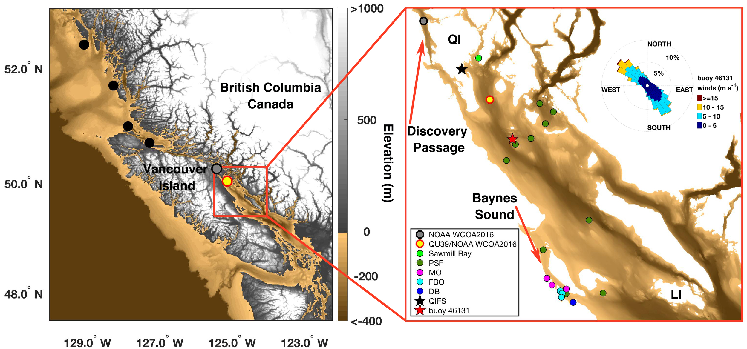
Figure 1. Sampling locations on the British Columbia (BC) coast (left) and in the Northern Salish Sea (NSS; red box in left and right). (Left) Shows locations occupied during the NOAA West Coast Ocean Acidification Cruise (WCOA2016) on the BC central coast (black), in Discovery Passage (gray), and in the NSS (red-outlined yellow circle). (Right) Shows locations in the NSS, defined here as waters extending from Quadra Island (QI) to Lasqueti Island (LI). The black star marks the Quadra Island Field Station (QIFS), and the red star marks Environment Canada weather buoy 46131. The Hakai Institute routinely samples the NSS station occupied during the NOAA WCOA2016 cruise (known as QU39). Additional sites were occupied by citizen science groups: light green dot = Sawmill Bay Shellfish Company, dark green dots = Pacific Salmon Foundation Citizen Science Program (PSF), magenta dots = Mac’s Oysters, Ltd. (MO), light blue dots = Fanny Bay Oysters (FBO), and dark blue dot = Vancouver Island University Deep Bay Field Station(DB). The wind rose in the right panel is hourly data from buoy 46131 collected between August 1997 to September 2018. Elevation shown in the left panel is from the Strait of Juan de Fuca 36 arc-second MHW Coastal Digital Elevation Model (https://data.noaa.gov/metaview/page?xml=NOAA/NESDIS/NGDC/MGG/DEM/iso/xml/541.xml&view=getDataView&header=none#Credit), and depth below sea surface in the right panel is from the British Columbia 3 arc-second Bathymetric Digital Elevation Model (https://data.noaa.gov/metaview/page?xml=NOAA/NESDIS/NGDC/MGG/DEM/iso/xml/4956.xml&view=getDataView&header=none). The color scale for depth below sea surface is the same between the two panels.

Marine CO₂ dynamics have not been well documented for the NSS beyond the information gained from periodic research cruises (Ianson et al., 2016) and limited underway observations from ships-of-opportunity (Evans et al., 2012; Tortell et al., 2012). A greater wealth of information exists for the central and southern Salish Sea, that collectively describe surface CO₂ system variability that is driven by large seasonal oscillations in primary productivity, freshwater delivery, and localized zones of intense tidal mixing (Feely et al., 2010; Evans et al., 2012; Tortell et al., 2012; Ianson et al., 2016; Fassbender et al., 2018). In deep Salish Sea water, total dissolved inorganic carbon (TCO₂) concentrations are high due to organic matter remineralization combined with restricted connectivity to the open continental shelf (Feely et al., 2010; Johannessen et al., 2014; Ianson et al., 2016). Nonetheless, as importantly noted by Fassbender et al. (2018), TA and TCO₂ concentrations are lower within the Salish Sea relative to the open North Pacific, however, the ratio of these two parameters (i.e., TA:TCO₂) is closer to 1, and therefore these waters are more weakly buffered (Egleston et al., 2010) than open North Pacific water. Weaker buffering capacity results in an amplified response of pH, CO₂ partial pressure (pCO₂), and aragonite saturation state (Ω_arag; where Ω_arag = [${\mathrm{CO}}_3^{2-}$][Ca²⁺]/K_sp(arag), and K_sp(arag) is the aragonite-specific solubility product) to changes in TCO₂. A TA:TCO₂ ratio near 1 also sets the tendency for seawater to be corrosive to aragonite (i.e., Ω_arag < 1). Seasonally, the entire Salish Sea water column has been observed to be corrosive to aragonite during winter, while during productive spring and summer months, Ω_arag increases in the surface layer (<20 m) to saturated levels (Feely et al., 2010; Ianson et al., 2016; Fassbender et al., 2018).

A number of organisms residing in the Salish Sea may be sensitive to currently observed Ω_arag and pH_T (total scale) conditions. Research has shown that Ω_arag during first shell development was a determining factor for growth and survival of larval Crassostrea gigas (Pacific oyster), and an Ω_arag value of 1.7 was determined to be the “break-even” point for commercial larvae production (Barton et al., 2012; Barton et al., 2015). C. gigas larval biomass production within the Whiskey Creek Hatchery on the Oregon coast was zero below this value (Barton et al., 2012). More detailed experimental work has revealed acute stress in juvenile C. gigas, Mytilus galloprovincialis (Mediterranean mussel), and M. californianus (California mussel) at Ω_arag values of 1.2 and 1.5, respectively (Waldbusser et al., 2014, 2015). Collectively, these studies highlight that Ω_arag levels above the thermodynamic threshold of 1 can negatively impact vulnerable early life stages of these species, with the duration and frequency of exposure to such adverse conditions also being important factors (Waldbusser and Salisbury, 2014). These vulnerable species reside in the NSS with Ω_arag values above these thresholds only in the surface layer during spring and summer months (Feely et al., 2010; Ianson et al., 2016; Fassbender et al., 2018). Similarly, pelagic species, such as Euphausia pacifica (krill; McLaskey et al., 2016) and Limacina helicina (thecosome pteropod; Bednarsek et al., 2017) may also be impacted by currently observed conditions. For instance, there is experimental evidence that E. pacifica larval development and survival is reduced at pH_T levels of 7.69 (McLaskey et al., 2016), values already seen in the region (Feely et al., 2010; Ianson et al., 2016; Fassbender et al., 2018). Efforts to model this area have focused on the southern domain (Moore-Maley et al., 2016; Bianucci et al., 2018), but highlight that the stability of favorable surface layer CO₂ conditions during summer can be disrupted by episodic variability.

In this paper, we will describe a growing NSS high-resolution dataset from the Hakai Institute’s Quadra Island Field Station (QIFS) that began in late 2014 in conjunction with other datasets collected by an array of observing activities that occurred during 2016 and 2017. These datasets collectively highlight important characteristics of the region, including perpetually low-Ω_arag at depth and large surface ocean variability across seasonal and sub-seasonal timescales. We also present estimates of anthropogenic CO₂ for NSS surface water spanning the start of the Industrial Revolution (e.g., 1765) to the end of the 21st century. Using this information, we assess the changes in Ω_arag and pH_T over ∼2.5 centuries and consider the passing of key biological thresholds during this period.

Materials and Methods

The approach applied here relied on developing a compilation of spatially- and seasonally distributed discrete seawater temperature, salinity, pCO₂, and TCO₂ measurements. The full marine CO₂ system was determined using these data as detailed below (see section “Discrete Seawater Sample Analyses”). A selected set of measurements was used to examine deep-water conditions within the NSS relative to the open continental shelf. Then, using the full suite of measurements, a relationship between alkalinity and salinity was constructed for the NSS. This relationship was then coupled with high-resolution surface measurements of salinity, temperature, and pCO₂ or pH_T collected at QIFS (see section “Autonomous Analytical Systems at the Quadra Island Field Station”) or from the Environment Canada weather buoy 46131 (see section “Buoy-of-Opportunity Continuous Observations”), respectively (Figure 1), to characterize surface CO₂ system variability over a 3.5-year period. Anthropogenic CO₂ was then estimated (see section “Estimation of Anthropogenic CO₂”) and used to assess the long-term trends in NSS surface water Ω_arag and pH_T. Ancillary datasets used in this manuscript are described in Supplementary Text 1.

Discrete Seawater Sample Analyses

Discrete seawater samples were collected during a number of field campaigns that occurred in 2016 and 2017 in the NSS (Figure 1 and Supplementary Table S1), including: (1) citizen science efforts by Sawmill Bay Shellfish Company, Fanny Bay Oysters, Mac’s Oysters Ltd., and the Pacific Salmon Foundation’s (PSF) Citizen Science Program; (2) occupations of the Hakai Institute’s oceanographic station QU39; (3) the 2016 United States National Oceanic and Atmospheric Administration (NOAA) West Coast OA Cruise (NOAA WCOA2016); and (4) shore-side sampling at the Vancouver Island University Deep Bay Marine Field Station. Seawater was collected using 350 mL amber soda-lime glass bottles that were filled either by hand (for the case of most citizen science groups) or using a Niskin bottle (for the cases of PSF, QU39, and NOAA WCOA2016) with care not to introduce bubbles. Sample bottles were rinsed three times with sample, filled from the bottom to leave ∼3 mL of headspace, fixed with 200 μl of a solution of saturated mercuric chloride, and crimp-sealed using polyurethane-lined metal caps. The effect of using soda-lime over borosilicate bottles was tested by comparing alkalinity determined (as described below) from triplicate surface and 500 m seawater samples stored in each bottle type for 100 and 126 days, respectively. No significant difference between the alkalinity of seawater stored in borosilicate or soda-lime glass bottles was evident at the end of either storage period (two sample t-test p-value for surface and 500 m water was 0.26 and 0.47, respectively). Triplicate sample sets were collected routinely in order to assess potential sampling uncertainty (estimated to be ∼8 μmol kg^-1 for triplicate alkalinity determinations computed over all datasets). Sampling by the citizen scientist organizations involved using NIST traceable thermometers (VWR PN 23609-176) to record in situ temperature with 0.2°C factory reported accuracy. In situ temperature and salinity were recorded by conductivity-temperature-depth (CTD) profilers either coupled with a Niskin bottle rosette (NOAA WCOA2016) or used just prior to Niskin bottle collection for samples collected by the Hakai Institute at station QU39. Niskin bottles deployed on a line for the PSF and QU39 field campaigns were tripped with messengers, and CTD data were extracted from the preceding profile for the Niskin bottle collection depth (for QU39 only). Niskin bottle target depth was determined using an A.G.O Environmental Ltd EWC-6 Electronic Wire Counter Module (or similar) and verified using RBRSolo² pressure sensors. Accuracy in hitting target depths was 2.6 ± 3.8 m, with largest inaccuracy occurring at the deepest depths. With the exception of the NOAA WCOA2016 data where CTD salinity co-occurred with the seawater sample collection, seawater sample salinity was measured using a YSI MultiLab 4010-1 with a MultiLab IDS 4310 conductivity and temperature sensor that is calibrated using the known salinity from CO₂ certified reference materials (CRMs; provided by A. Dickson at Scripps Institute of Oceanography). The uncertainty in salinity determinations from the calibrated probe was estimated to be 0.11 based on the standard deviation about a mean difference of 0.01 between measured and known CRM salinity and the standard deviation between station QU39 sample YSI salinity and CTD salinity.

For all the above listed datasets, discrete seawater sample analysis for TCO₂ and pCO₂ was conducted on a Burke-o-Lator (BoL) pCO₂/TCO₂ analyzer at QIFS by acidification with 1 N hydrochloric acid followed by flow-balanced gas stripping for TCO₂ (Hales et al., 2004; Bandstra et al., 2006) and recirculated-headspace gas equilibration for pCO₂ (Hales et al., 2004). Our protocol for TCO₂ and pCO₂ analysis followed methods published previously (Hales et al., 2005; Barton et al., 2012; Hales et al., 2016) with some slight modification to the degree at which CRMs were processed and how quality control was conducted¹. CO₂ mole fractions (xCO₂) were detected in the analytical gas stream, either evolved following acidification and stripped for the TCO₂ analysis stream or recirculated through the pCO₂ headspace gas loop, by non-dispersive infrared (NDIR) absorbance using a gas analyzer (LI-COR LI840A CO₂/H₂O) housed within the BoL’s electronics box. Both TCO₂ and pCO₂ were measured from the same seawater sample, with TCO₂ measured first in a process that took ∼2.5 min and consumed ∼50 mL of sample. TCO₂ measurements were calibrated using liquid standards, which were solutions of Na₂CO₃ and NaHCO₃ in deionized water that had been prepared to have target TCO₂ values (nominally 800, 1600, and 2400 μmol kg^-1) with alkalinity adjusted to give solution pCO₂ near that of ambient room air. The liquid standards were stored in gas-impermeable bags, and were analyzed, along with a set of gas standards (see section “Autonomous Analytical Systems at the Quadra Island Field Station”), in conjunction with each group of samples analyzed in a day. The order of analyses that would occur was: (1) gas standards, (2) liquid standards, (3) triplicate TCO₂ analysis of a CRM bottle, (4) TCO₂ and pCO₂ analyses on a battery of typically 20–30 samples, (5) triplicate TCO₂ analysis of the same CRM bottle as well as a pCO₂ analysis following the last TCO₂ measurement (that had been resealed between analyses), (6) liquid standards, and finally (7) gas standards. In this way, gas and liquid calibration curves were generated at the start and end of a sample analysis sequence, linearly interpolated over the time period of sample analysis (usually <8 h), and then used to calibrate the TCO₂ and pCO₂ analyses. Post-calibration TCO₂ samples were converted to units of μmol kg^-1 using the sample density based on the salinity and temperature at the time of analysis. Sample temperature at the time of analysis was recorded using NIST traceable thermometers (VWR PN 23609-176). pCO₂ was measured with the BoL following the TCO₂ analysis by recirculating a closed loop of headspace gas through the seawater sample (by bubbling with an aquarium air diffuser) for a period of 10 min in order to ensure full equilibration of the headspace gas. Post-calibration pCO₂ measurements were converted from xCO₂ to pCO₂ using ambient laboratory total pressure. A correction factor was applied to the TCO₂ data based on the analyses of CRMs of known TCO₂ content (batch numbers 151, 157, 169, and 174). Each triplicate CRM run in the analysis sequence listed above was averaged, and the ratio of known to measured average TCO₂ content was interpolated over the time period of the analysis sequence and subsequently used to correct measured sample TCO₂. Typical correction factors for TCO₂ analysis range between 0.99 and 1.01, with deviations from the ideal value of 1.00 related to the accuracy of liquid standard preparation. The standard deviation in CRM triplicate runs was used as a metric of analytical uncertainty, computed here to be 0.3%. Analysis temperature, salinity, TCO₂, and pCO₂ were used to compute seawater sample alkalinity, however, a final adjustment was needed to obtain the correct alkalinity that accounted for the change in TCO₂ induced by the bubbling of headspace gas through the sample volume (Wanninkhof and Thoning, 1993). In situ pCO₂, pH_T, and Ω_arag were then computed using the MATLAB version of CO2SYS (Van Heuven et al., 2011) with alkalinity, TCO₂, in situ temperature, salinity, and pressure as inputs. Calculations were done with nutrient concentrations omitted, and using the carbonic acid dissociation constants of Lueker et al. (2000), the bisulfate dissociation constant of Dickson et al. (1990), the boron/chlorinity ratio of Uppström (1974), and the aragonite solubility constant from Mucci (1983) with no adjustment for a potential non-zero Ca²⁺ intercept. Alkalinity (Alk_inorganic) consisted of carbonate, bicarbonate, borate, hydroxide, and hydrogen ions, all of which can be calculated from the direct measurements of pCO₂ and TCO₂. Note that TA is Alk_inorganic plus the contributions for phosphate, silicate, and organic acids, which here are assumed to be negligible such that TA ≈ Alk_inorganic. Lastly, there is no parameter-specific CRM available for pCO₂, therefore we assessed the analytical uncertainty of that measurement based on the comparison of known CRM TA and that calculated from measured TCO₂ and pCO₂. The comparison between certified and calculated TA points to an analytical uncertainty of ∼1.5%, however, we note that this determination is based on pCO₂ analyses of CRM bottles that had been opened and resealed <8 h before analysis. Also, the headspace in the CRM had increased since opened as well as flushed with ambient room air. Because of these reasons, we expect that the uncertainty listed above is over- estimated and that the true uncertainty is likely ≤1%.

Autonomous Analytical Systems at the Quadra Island Field Station

Near-continuous pCO₂ measurements made on surface (1 m) seawater from Hyacinthe Bay, adjacent to the QIFS (Figure 1), were collected using two analytical systems over the course of this study: (1) the Sunburst Sensors Shipboard Underway pCO₂ Environmental Recorder (SUPERCO₂) from December 18, 2014 to April 6, 2016, and (2) the BoL from April 6, 2016 to June 1, 2018. Seawater pCO₂ data produced by both systems were calculated from corrected measurements of wet air xCO₂ made following standardization protocols described by Pierrot et al. (2009) with the system theory and calculations presented by Hales et al. (2004) and Evans et al. (2015). Seawater was drawn from a 2-inch diameter polypropylene tube positioned approximately 50 m from shore at ∼150 l min^-1 using a Pentair Aquatic Eco-systems Sparus 3HP pump (or similar). Most seawater was diverted back to sea, while an analysis seawater stream was drawn tangentially off the main supply and diverted through the instrumentation configured within a shore-side flow-through laboratory at ∼4 l min^-1. Within the laboratory, unaltered seawater continuously flowed first through a Sea-Bird Electronics SBE 45 MicroTSG Thermosalinograph, and then through a seawater equilibrator before being returned to sea.

Equilibrator design differed slightly between the two systems. The SUPERCO₂ used both primary and make-up air showerhead equilibrators (Takahashi, 1961) in order to pre-equilibrate any (make-up) air drawn into the primary equilibrator via the presence of a slight vacuum pressure. The BoL pre-equilibrated make-up air by direct contact with seawater running vertically down the wetted-wall of the equilibrator drain pipe, further isolated from the ambient air by a ‘P trap’ to the ultimate water exit from the system. The BoL equilibrator did not have a showerhead, but instead diverted incoming seawater over a flat plate surrounded by porous tubing that delivered headspace gas with vigorous bubbling into the seawater stream. Both equilibrator designs were found to have response times (e-folding times) on the order of 2 min determined by sequentially injecting high and low concentration standard gas directly into the equilibrators and tracking the return to equivalent pre-disturbance levels. Equilibrators for both systems supplied equilibrated carrier gas (marine air) to a LI840A housed within an electronics box. The SUPERCO₂ system diverted a split from the recirculation headspace gas flow at a rate of ∼50 ml min^-1, which was made-up through the pre-equilibrated make-up air line, while the BoL system circulated the entire headspace flow through the LI840A in a quasi-closed-loop configuration. Pressure and temperature were continuously monitored in the equilibrators using either Honeywell or Omega Pressure Sensors and Fast Response Resistance Temperature Detectors, respectively. Unaltered marine air was drawn from 0.25-inch polyethylene tubing that connected a vented water trap positioned outside of the shore-side laboratory to the analytical systems coincident with the detector standardization sequence. The detector was calibrated with gasses of known gravimetric mol/mol mixing ratio of CO₂ in ultrapure air. Equilibrated carrier gas, standard gasses of known mixing ratio (three for the SUPERCO₂ = 150.4, 453, and 750 ppm; four for the BoL = 153.3, 451, 752, and 1515 ppm; formerly Scott-Marin Inc., now Praxair Distribution Inc.), and unaltered marine air were all plumbed to provide gas flow to the electronics boxes of both systems. Computers with National Instruments LabVIEW software controlled data acquisition from the thermosalinograph, the pressure and temperature sensors, and the LI840A, while also controlling Valco Instruments Co. Inc. (VICI) multi-port actuators that cycled between the gas streams plumbed to the electronics box. None of the gas streams were dried prior to analysis, and measurements were made at 0.5 and 1 Hz on the SUPERCO₂ and BoL, respectively.

The prescribed measurement schemes controlled by the software differed slightly between the two systems. Software on the SUPERCO₂ was initially set to supply equilibrated carrier gas from the primary equilibrator to the LI840A continuously for 240 min, then cycle the actuators to consecutively allow the three standard gas streams and unaltered marine air to be measured for 90 s each at ∼100 ml min^-1 before returning to sample the carrier gas equilibrated with seawater pCO₂. After the 1st weeks of operation, the time between standardization sequences was increased to once per day as the high degree of standardization typically employed on research cruise was not necessary. From each sequence of standard gas measurements, the final 20 s of data in the 90 s interval before the actuator changed position was averaged and then used to construct a linear fit of the LI840A response to each gas standard in the sequence. These steps were conducted using custom MATLAB programs. LabVIEW software controlling the BoL cycled through gas standards and unaltered marine air every 720 min, at which time gas flowed during each step of the sequence for 60 s before a 20 s averaging window occurred. Unlike for the SUPERCO₂, LabVIEW software running the BoL computed the linear fit of a calibration sequence and stored this information in a calibration file. Corrected atmospheric xCO₂, as part of the aforementioned gas standard sequence, and atmospheric pressure measurements from the LI840A were used to compute atmospheric pCO₂ and stored in the BoL calibration file. The linear fits constructed with data from both systems for each calibration sequence were then interpolated in time between standard gas sequences in order to produce temporally resolved calibration functions. These functions were then used to calibrate the raw xCO₂ measurements of both the seawater equilibrated carrier gas and unaltered marine air, with an adjustment on the order of 1%. Corrected seawater xCO₂ was subsequently adjusted for any under- or over-pressurization in the equilibrator using the ratio of equilibrator-to-vented LI840A cell pressure, and then converted to pCO₂ using atmospheric pressure measured by the LI840A. The seawater pCO₂, temperature, and salinity (reported here on the Practical Salinity Scale, PSS-78; dimensionless) data were quality controlled by removing obvious aberrant measurements, and then bin-averaged in 5-min interval bins.

Although residence time within the mostly submerged seawater supply line was minimal (∼2 min), warming was assessed on two separate occasions by comparing temperature from the thermosalinograph with measurements made using a SBE 56 Temperature Sensor affixed to the end of the seawater intake line during two ∼20-day periods starting in early October and late November 2017. The SBE 56 data revealed a trivial amount of warming (averaging ∼0.2 ± 0.1°C over both ∼20-day deployments) that would result in a slight positive bias for pCO₂ by <1%. This bias, combined with a consistently observed 2 ppm uncertainty in xCO₂ determinations revealed by the comparison of calibrated standard gas readings to the known values, equated to ∼1.5% uncertainty for pCO₂. CO₂ system parameters were then computed using the bin-averaged data with Alk_inorganic estimated using a regional Alk_inorganic-salinity relationship using a MATLAB version of CO2SYS (Van Heuven et al., 2011) with the series of constants described previously.

Buoy-of-Opportunity Continuous Observations

A Sea-Bird Electronics SeaFET V1 Ocean pH sensor was used during two deployments on the Environment Canada weather buoy 46131 (Figure 1) between summer and autumn in 2016 and 2017. These deployments occurred in collaboration with PSF who deployed a Sea-Bird Electronics SBE 37 MicroCAT to record seawater temperature and salinity from the platform. Both units were placed in protective stainless steel cages and hung off the surface buoy with chain to 1 m depth. Copper tape and copper guards were used to prevent biofouling of the units during deployment. The SeaFET went through a near 10-day period of pre-conditioning within a test tank filled with NSS surface water prior to each deployment. At this stage, the response of both internal and external electrodes was tracked and the deployment settings were configured. The SeaFET was set to sample every 30 min throughout each deployment. Here, we only report data generated using the SeaFET’s internal electrode.

Once deployed, the SeaFET was allowed to condition for a period of 10–14 days before discrete seawater samples were collected adjacent to the sensor for TCO₂ and pCO₂ analysis on the QIFS BoL. Discrete seawater samples were collected using Niskin bottles deployed to 1 m depth alongside the sensor at the time of a sampling event, and analyzed as described above. Calibration coefficients for each electrode were then re-calculated using the average in situ pH_T of triplicate discrete samples and the corresponding electrode voltage reading (equations detailed in Sea-Bird Scientific SeaFET Product Manual 2.0.0.), resulting in an adjustment from the factory calibration of ∼0.03%. The calibration coefficients were calculated following any major sensor maintenance such as battery change or annual service, which occurred four times over the course of the deployments. Additional discrete samples were collected during service visits approximately once every 2 months throughout the deployment period to validate the single-point calibration. The offset between validation sample and SeaFET pH was 0.005 ± 0.001 averaged over both deployments, indicating no observable drift. The in situ calibration coefficients, along with temperature data from the co-located SBE 37 were used to convert SeaFET electrode voltage readings to in situ pH_T measurements. Same as for the QIFS analytical systems, CO₂ system parameters were then computed using a regional Alk_inorganic-salinity relationship with the series of constants described previously and a MATLAB version of CO2SYS (Van Heuven et al., 2011).

Estimation of Anthropogenic CO₂

The ΔTCO₂ approach (Sabine et al., 2002; Takeshita et al., 2015; Pacella et al., 2018) was employed to calculate anthropogenic CO₂ in NSS surface water. This approach makes the following assumptions: (1) the difference between surface seawater TCO₂ and the TCO₂ level expected if surface seawater pCO₂ were in equilibrium with the atmosphere at the current TA, termed ΔTCO_2,diseq, is constant in time, (2) variability in temperature, salinity, and TA is also constant in time. The ΔTCO₂ approach has advantages over the commonly used ΔpCO₂ approach (Feely et al., 2010; Harris et al., 2013; Evans et al., 2015; Hales et al., 2016; Sutton et al., 2016; Pacella et al., 2018) because it captures Revelle Factor-driven changes in seawater pCO₂ seasonal dynamic ranges (Fassbender et al., 2018; Feely et al., 2018; Landschützer et al., 2018; Laruelle et al., 2018), meaning that amplified changes in pCO₂ per unit change in TCO₂ are captured, thereby subsequently not manifested in amplified unrealistic TCO₂ variability and so likely producing a more robust estimate of anthropogenic CO₂. We used 14-day low-pass (LOESS) filtered daily data from 2017 to compute ΔTCO_2,diseq with the following formulation:

$$\mathrm{\Delta }{\mathrm{TCO}}_{2,\mathrm{diseq}}={\mathrm{TCO}}_{2,2017}-{\mathrm{TCO}}_2\mathrm{\hspace{0.17em}}(\mathrm{atm}\mathrm{\hspace{0.17em}}{\mathrm{pCO}}_{2,2017},\mathrm{\hspace{0.17em}}\mathrm{TA})$$

where TCO₂ (atm pCO_2,2017, TA) is the TCO₂ concentration calculated at the 2017 mean atmospheric pCO₂ and TA levels. Then using this ΔTCO_2,diseq term, we computed TCO₂ for each day of each year between 1765 and 2100 as:

$${\mathrm{TCO}}_{2,\mathrm{yr}}={\mathrm{TCO}}_{2,\mathrm{yr}}\mathrm{\hspace{0.17em}}(\mathrm{atm}\mathrm{\hspace{0.17em}}{\mathrm{pCO}}_{2,\mathrm{yr}},\mathrm{\hspace{0.17em}}\mathrm{TA})+\mathrm{\Delta }{\mathrm{TCO}}_{2,\mathrm{diseq}}$$

where TCO_2,yr (atm pCO_2,yr, TA) was determined using atmospheric pCO₂ from the RCP 8.5 (Riahi et al., 2011) “business as usual” record from 1765 to 2100 (Supplementary Text 1). Finally, anthropogenic CO₂ for each day of each year was calculated as:

$$\mathrm{anthropogenic}\mathrm{\hspace{0.17em}}{\mathrm{CO}}_2={\mathrm{TCO}}_{2,\mathrm{yr}}-{\mathrm{TCO}}_{2,1765}$$

Uncertainty in calculated anthropogenic CO₂ has been shown to be 10% (Sabine et al., 2002).

Results

NSS Alk_inorganic-Salinity Relationship and CO₂ System Uncertainties

Over 250,000 marine CO₂ system measurements have been collected over the course of this study spanning December 18, 2014 to June 1, 2018 (Supplementary Table S1). The data collected highly resolve each season over 3.5 years, with the majority of observations occurring in the surface layer where the largest seasonal dynamic range was evident. The establishment of a NSS Alk_inorganic-salinity relationship was an integral tool developed using the discrete datasets and utilized with the continuous records. A total of 1360 seawater samples collected over the seven field campaigns and spanning the full water column, all seasons (Supplementary Table S1), and a broad range of salinity (1.4–30.9) conditions were used to construct this relationship (Figure 2). The uncertainty in this relationship, as indicated by the root mean square error (RMSE), was 22.47 μmol kg^-1. The Alk_inorganic-salinity relationship presented here spanned a much broader salinity range than a comparable TA-S relationship developed using data from the coastal zone around Washington State including the southern Salish Sea [(Fassbender et al., 2016); salinity 20–35]. These two relationships are more consistent at the higher salinity range and diverge at the lower salinity range.

FIGURE 2

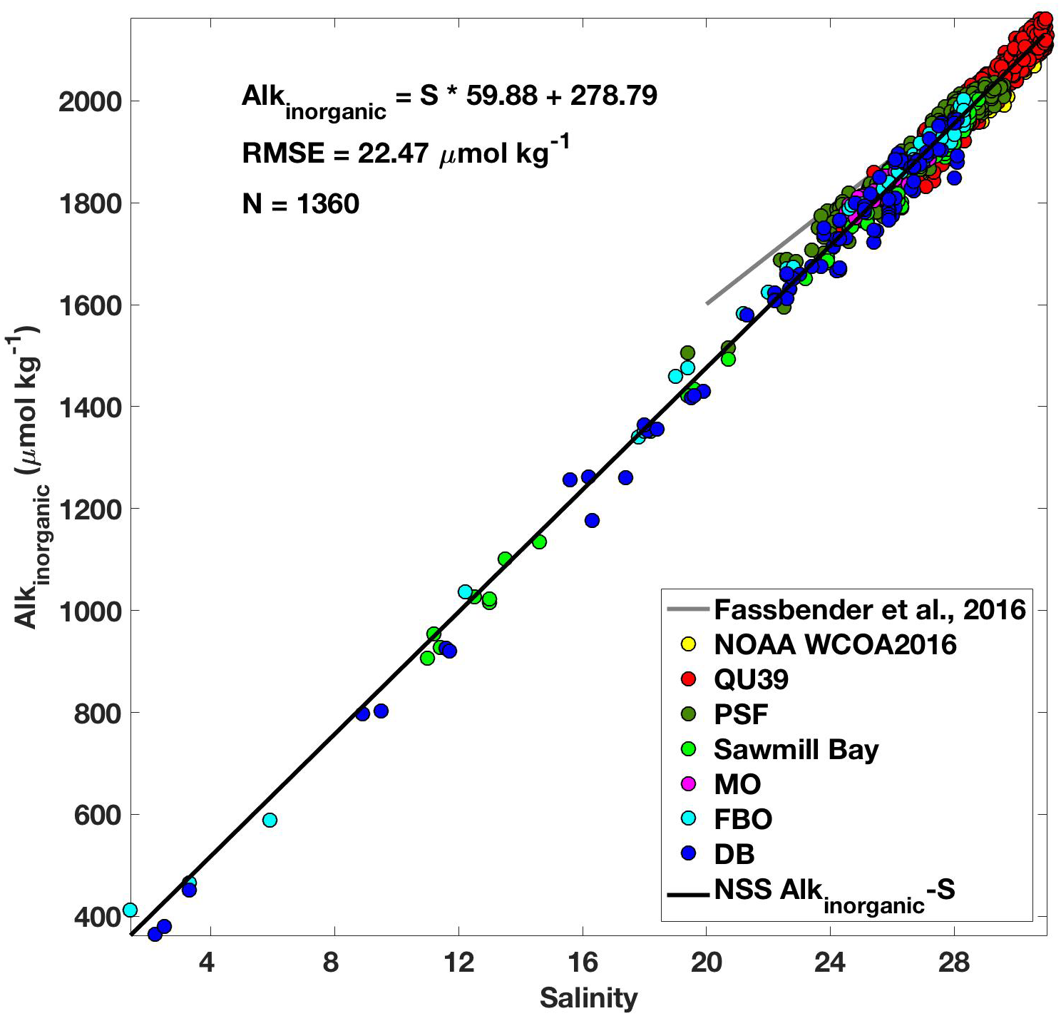
Figure 2. Relationship between alkalinity (Alk_inorganic; μmol kg^-1) and salinity (black line; Alk_inorganic = S ^∗ 59.88 + 278.79; RMSE = 22.47 μmol kg^-1) developed using 1360 discrete measurements of pCO₂, TCO₂, temperature, and salinity collected at oceanographic and aquaculture sites in the NSS (color matched with position in Figure 1) between 2016 and 2017. Also shown for comparison is the relationship from Fassbender et al. (2016; gray line) that was constructed using data collected over a salinity range from 20 to 35.

The NSS Alk_inorganic-salinity relationship was used with direct CO₂ system measurements (either pCO₂ or pH_T) to determine the full marine CO₂ system. However, it is important to consider how our measurement and relationship uncertainties propagate to uncertainties in the derived parameters (Supplementary Table S2). Using the reported measurement uncertainties detailed above with a MATLAB CO2SYS error propagation routine that includes uncertainty in the carbonic acid dissociation constants (Orr et al., 2018), we determined the uncertainty in derived CO₂ system parameters relative to the mean conditions observed during this study. The full CO₂ system was determined by three sets of parameter pairs: (1) continuous pCO₂ with Alk_inorganic derived from our regional Alk_inorganic-salinity relationship [Alk_inorganic(S); Figure 2], (2) continuous pH_T with Alk_inorganic (S), and (3) discrete TCO₂ and pCO₂. Of these three sets of pairings, Ω_arag determined by continuous pH_T from the SeaFET sensor combined with Alk_inorganic (S) had the largest uncertainty of 0.039 or 3%. Unsurprisingly, the discrete TCO₂ and pCO₂ pair had the lowest Ω_arag uncertainty of 0.031 or 2%. The close agreement between uncertainties from all three pairings (Supplementary Table S2), even with an RMSE of 22.47 μmol kg^-1 in the Alk_inorganic-salinity relationship (Figure 2), indicated that uncertainty in continuous pCO₂ or pH was a larger contributor than uncertainty in our Alk_inorganic-salinity relationship to the uncertainty in derived Ω_arag (Fassbender et al., 2016). These reported uncertainties were nearly an order of magnitude lower than the ±0.2 Ω_arag uncertainty threshold prescribed by the California Current Acidification Network (C-CAN; McLaughlin et al., 2015) and the Global Ocean Acidification Observing Network (GOA-ON; Newton et al., 2015) required for “weather” quality data that can link changes in marine ecosystems to changes in the marine CO₂ system.

NSS Deep Water Conditions Relative to the Open Continental Shelf

Measurements made at depth (i.e., >50 m) during both the NOAA WCOA2016 cruise and from occupations of oceanographic station QU39 illustrate a key aspect of deep water in the NSS that sets this domain apart from conditions found at similar depths on the open continental shelf (Figure 3); the NSS was observed to be continually corrosive below the depth zone influenced by surface dynamics. Six near-shore stations were occupied during the NOAA WCOA2016 cruise in a transect that spanned the open continental shelf, Discovery Passage, and the NSS (Figure 1). Surface variability across the transect reflected a spectrum of conditions related to CO₂ drawdown by phytoplankton, freshwater dilution, and vertical mixing that extended deeper into the water column on the open continental shelf but limited to <50 m. Below this depth, salinity, Alk_inorganic, and TCO₂ were all higher on the open continental shelf compared to values found within the NSS (Figure 3). However, Alk_inorganic:TCO₂ was lower in the NSS, and this condition is a key determinant in setting pCO₂, pH_T, and Ω_arag levels. At salinity at and above the NSS mean (26.26) with Alk_inorganic:TCO₂ near 1, pH_T and Ω_arag have nominal values of 7.5 and 0.6, respectively. Therefore, it is unsurprising that the water column below the surface layer (>50 m) with Alk_inorganic:TCO₂ near 1 has Ω_arag near 0.6 (Figure 3). Alk_inorganic:TCO₂ equal to 1 also marks the condition where pCO₂, pH_T, and Ω_arag will change the most with incrementally increasing TCO₂ (Egleston et al., 2010). As anthropogenic TCO₂ addition continues beyond this equivalency point, per unit changes in pCO₂, pH_T, and Ω_arag will decrease. The conditions found at depth during the NOAA WCOA2016 cruise closely align with the seasonally resolved average for ≥150 m samples collected at station QU39 between January 2016 and December 2017 (Figure 3; n = 206), indicating perennially low-Ω_arag deep water in the NSS.

FIGURE 3

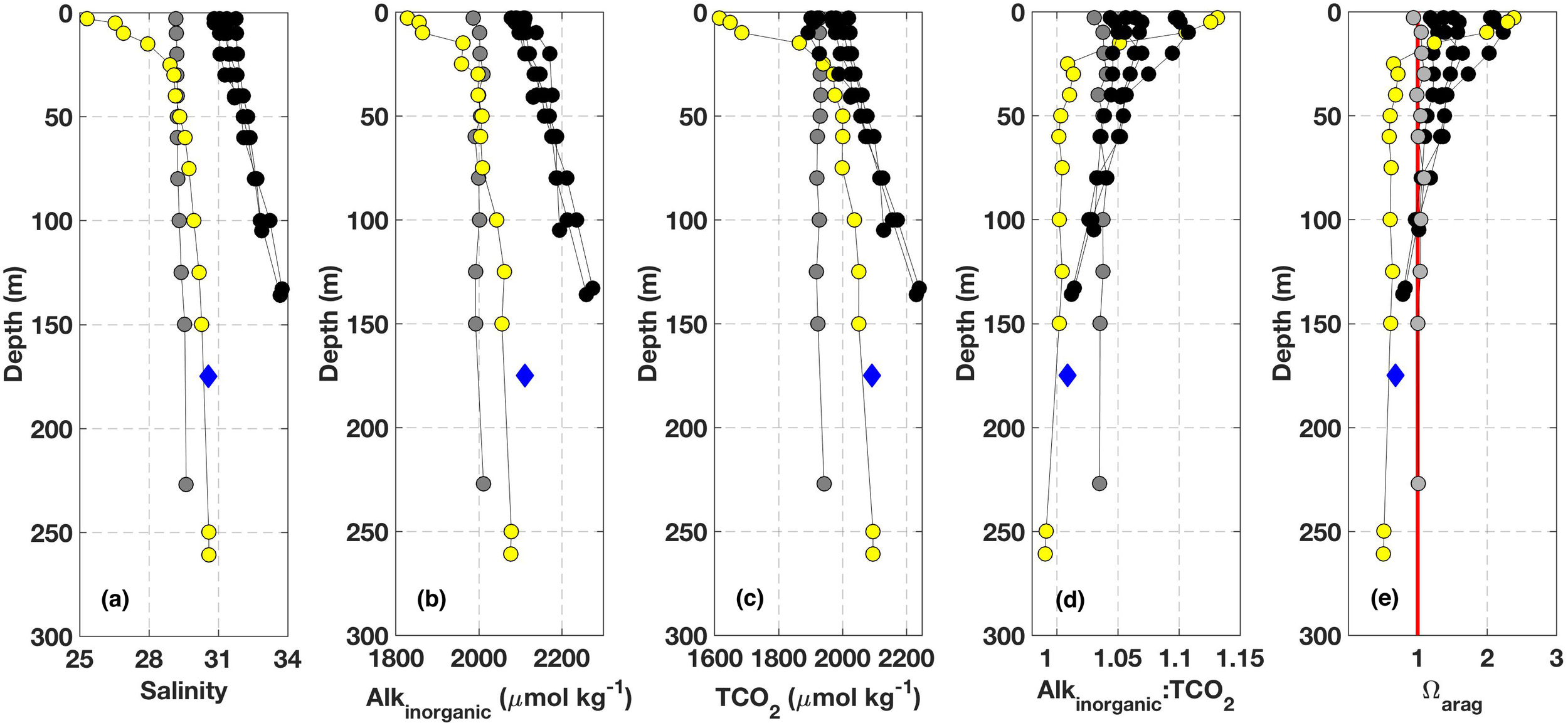
Figure 3. Observations from the NOAA WCOA2016 cruise in June 2016 color-coded by area as shown in Figure 1: data from the BC open continental shelf are black, the data from Discovery Passage are gray, and data from the NSS (QU39) are yellow. The data shown are: (A) salinity, (B) Alk_inorganic (μmol kg^-1), (C) TCO₂ (μmol kg^-1), (D) Alk_inorganic:TCO₂, and (E) Ω_arag. The vertical red line in (E) marks Ω_arag = 1. Also shown are averages from seasonally resolved data collected at station QU39 from depths ≥ 150 m between January 2016 and December 2017 (blue diamonds; n = 206). The deep-water averages (±standard deviation) for salinity, Alk_inorganic, TCO₂, Alk_inorganic:TCO₂, and Ω_arag were 30.58 ± 0.25, 2112 ± 24 μmol kg^-1, 2093 ± 31 μmol kg^-1, 1.009 ± 0.008, and 0.68 ± 0.09, respectively.

NSS Surface Water Variability

Variability was pronounced in NSS surface water, with large dynamic ranges of temperature, salinity, and CO₂ system parameters on seasonal and sub-seasonal time scales. The seasons were defined here with December through February as winter, March through May as spring, June through August as summer, and September through November as autumn. SST varied from ∼6°C in winter to ∼20°C in summer, while salinity was less seasonally varying with low values, minima near 20, during short-lived freshwater events and high values, maxima near 30, during summertime mixing events (either vertically mixed locally or transported laterally to the measurement location) that drove concurrent low-pH_T and high-pCO₂ conditions. Wintertime pCO₂ and pH_T were near 700 μatm and 7.8, respectively, with generally lower variability relative to the summer months. The standard deviation of wintertime pCO₂ was less than 70 μatm for all years. The transition from winter CO₂ conditions in spring was rapid and marked by the occurrence of the spring phytoplankton bloom that drew down surface pCO₂ well below equilibrium with the atmosphere. The timing of this initial drawdown varied by ∼6 weeks; observed to occur as early as the start of March in 2015 and as late as late April in 2017. Spring bloom-driven low-pCO₂ conditions were disrupted in 2015, 2016, and 2018 by late season southeasterly winds. Summertime levels were generally more variable, with seasonal pCO₂ standard deviations of 140 and 100 μatm in 2015 and 2016, respectively. During 2017, summertime variability was lower, however, with a seasonal standard deviation of 40 μatm. pCO₂ and pH_T levels during periods of assumed highest primary productivity and subsequent CO₂ drawdown reaching to near 100 μatm and up to 8.50, respectively. During observed summertime short-lived mixing events, pH_T went down to as low as 7.65 and pCO₂ up to near 1000 μatm. These seasonal and sub-seasonal signals were evident in both the QIFS and buoy 46131 records, platforms located ∼26 km apart (Figure 1), which provided an indication of spatial coherence in the observed patterns (Figure 4). However, summertime high-CO₂ events did not occur each year; summertime surface pCO₂ in 2015 and 2016, but not in 2017, episodically reached or exceeded levels observed during wintertime (see section “The Lack of High-CO₂ Summertime Conditions in 2017”). Autumn marks the transition back to wintertime conditions, however, evidence of late season pCO₂ drawdown likely associated with a phytoplankton bloom occurred in 2015.

FIGURE 4

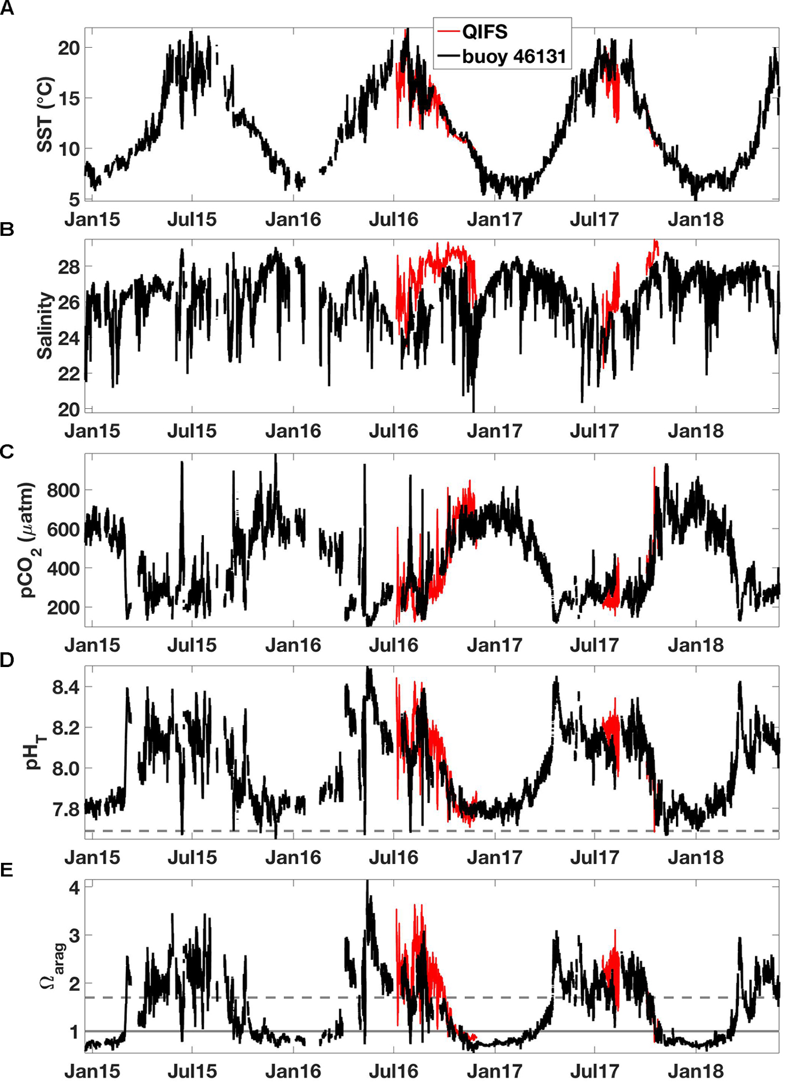
Figure 4. High-resolution observations of (A) SST (°C), (B) salinity, (C) pCO₂ (μatm), (D) pH_T, and (E) Ω_arag from the QIFS (black) and Environment Canada buoy 46131 (red). The horizontal line in (D) marks pH_T = 7.69, and the horizontal lines in (E) mark Ω_arag = 1 (solid gray) and Ω_arag = 1.7 (dashed gray).

Combined meteorological and oceanographic records from QIFS and buoy 46131 over the duration of a high-CO₂ event in July 2016 revealed the significance of wind forcing as a driver for the occurrence of vertical mixing and subsequently observed large CO₂ system variability (Figure 5). Using the wind records from buoy 46131 adjusted to 10 m (Hsu et al., 1994), wind stresses were computed along the main axis of the NSS (Figure 1) with drag coefficients determined using the relationship of Smith et al. (1991). Wind stresses became negative (indicating northwesterly winds) on July 25, and strengthened over a ∼5-day period. The surface ocean response to the intensifying negative along-axis wind stress was a concurrent decrease in SST, an increase in salinity, and a >400 μatm increase in pCO₂ at both QIFS and buoy 46131 (Figure 5), which were indications of strong vertical mixing. pH_T dropped at QIFS to below the observed wintertime levels (7.65), and surface water Ω_arag ≤ 1 was evident at both sites prior to the wind stress abating. By August 1, intense along-axis wind stress associated with strong (i.e., >5 m s^-1) wind speeds had completely abated, with pCO₂, pH_T, and Ω_arag returning to near pre-disturbance levels by August 4. However, salinity stayed elevated and SST warmed only marginally by 2–3°C during this period of rapidly transitioning CO₂ system parameters. A similar vertical mixing and high-CO₂ event was observed in 2015, and showed a consistent time evolution to the 2016 event described above (although CO₂ observations were limited to QIFS; Supplementary Figure S1). Satellite SST observations captured both the 2015 and 2016 events and showed 6–8°C of cooling that occurred broadly over the entire NSS over ∼6 days (Figure 6 and Supplementary Figure S2).

FIGURE 5

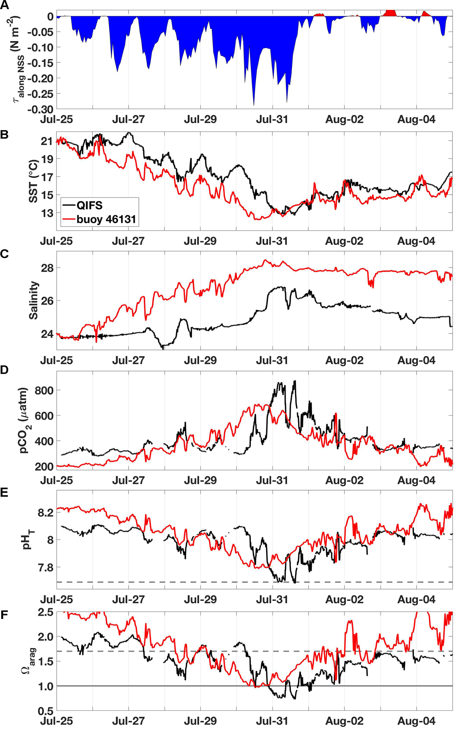
Figure 5. Observations made during the July 2016 high-CO₂ event, including: (A) along-axis wind stress (τ_{along NSS}; N m^-2) from buoy 46131, (B) SST (°C) from QIFS and buoy 46131, (C) salinity from QIFS and buoy 46131, (D) seawater pCO₂ (μatm) from QIFS and buoy 46131, (E) pH_T from QIFS and buoy 46131, and (F) Ω_arag from QIFS and buoy 46131. All QIFS data are black while buoy 46131 data are red. The horizontal line in (E) marks pH_T = 7.69, and the horizontal lines in (F) mark Ω_arag = 1 (solid gray) and Ω_arag = 1.7 (dashed gray).

Anthropogenic CO₂ in NSS Surface Water

Calculations of annual mean anthropogenic CO₂ in NSS surface water show a steady increase since the Industrial Revolution (∼1765) with intensifying growth rates beginning after 1950 (Supplementary Figure S3) that reflects the evolving pace of increasing atmospheric CO₂ levels. Annual minima and maxima of anthropogenic CO₂ values, with variance largely associated with the vertical mixing of sub-surface water with a lower anthropogenic CO₂ content, diverged from the corresponding annual means toward the end of the 21st century. As mentioned previously, these estimates were based on 2017 observations when observations of high-CO₂ were reduced, and hence lack of strongest vertical mixing events that would accompany the lowest anthropogenic CO₂. However, calculations of mean anthropogenic CO₂ were less sensitive than the variance to the year of input data used in the computation. Calculations using 2015 data resulted in a slightly broader range of annual minima and maxima values with no significant difference in mean estimates. Mean anthropogenic CO₂ estimated for 2018 was 49 ± 5 μmol kg^-1. By comparison, the mean value for 2008 was 41 ± 4 μmol kg^-1 and close to the value reported by Feely et al. (2010) for the Main Basin in Puget Sound during summer (36 μmol kg^-1; Supplementary Figure S3). The difference between these two estimates, which is marginally outside of the expected 10% uncertainty, may be related to one or both of the following two factors: (1) the difference between estimating anthropogenic CO₂ using the ΔpCO₂ approach versus the ΔTCO₂ approach (see Supporting Information by Pacella et al., 2018), and (2) building estimations using high-resolution datasets versus data from infrequent research cruises. However, it is important to note that these determinations fall below estimated levels for BC open continental shelf surface water (Feely et al., 2016), and that differences in buffering capacity between the open continental shelf, Puget Sound, and the NSS contribute to driving the expected regional differences in estimated anthropogenic CO₂ (Sabine et al., 2004).

Discussion

CO₂ Dynamics in the NSS

The rigorous evaluation of NSS CO₂ dynamics presented here was reliant on dedicated high-resolution monitoring sites combined with frequent and spatially distributed discrete sample collection by a number of organizations. This combination of assets produced data that highlight perpetually corrosive conditions at depth as well as dynamic variability across a range of time scales at the surface. Continuously corrosive conditions in deep water is an important feature of this setting, as a number of marine organisms have experimentally been shown to exhibit sensitivities, in terms of reduced calcification (Kroeker et al., 2013; Bednarsek et al., 2017) and slower growth (McLaskey et al., 2016), at the currently observed levels. Perpetually corrosive conditions have not been seen on the open continental shelf, where deep water (165 m) Ω_arag can vary from 0.8 to 2.4 (Harris et al., 2013). An Alk_inorganic:TCO₂ near 1 sets the corrosive state of NSS deep water, and high organic carbon input (Johannessen et al., 2014) and annual deep water renewal (Masson, 2002; Pawlowicz et al., 2007) both act to maintain a state of elevated TCO₂ relative to Alk_inorganic. This pattern is consistent with observations made in Puget Sound (Feely et al., 2010) where deep water exchange with the open continental shelf is restricted and corrosive conditions dominate. Such corrosive hot spots likely serve as important areas to gauge organismal and ecosystem response to OA.

Baseline information across a broad range of time scales, afforded by continuous high-resolution datasets such as shown here, is needed to understand current marine CO₂ “weather” conditions and how these might relate to projected CO₂ “climate” scenarios (Waldbusser and Salisbury, 2014). Surface-oriented forcing (i.e., wind-driven vertical mixing, seawater CO₂ drawdown via primary productivity, freshwater addition and stratification) drove large dynamic ranges of surface water CO₂ parameters in the NSS (Figure 4). Such surface dynamics are not unique to this area, and similarly large ranges have been reported for the southern Salish Sea (Feely et al., 2010; Ianson et al., 2016; Fassbender et al., 2018). However, information has been scarce on the importance of high-frequency variability; the summertime wind events shown here in the NSS resulted in CO₂ system “weather” variation in pCO₂, Ω_arag, and pH_T that surpassed the seasonal dynamic ranges of these parameters in less than a week (Figure 4) and likely over the entire domain, as indicated by satellite SST observations (Figure 6).

FIGURE 6

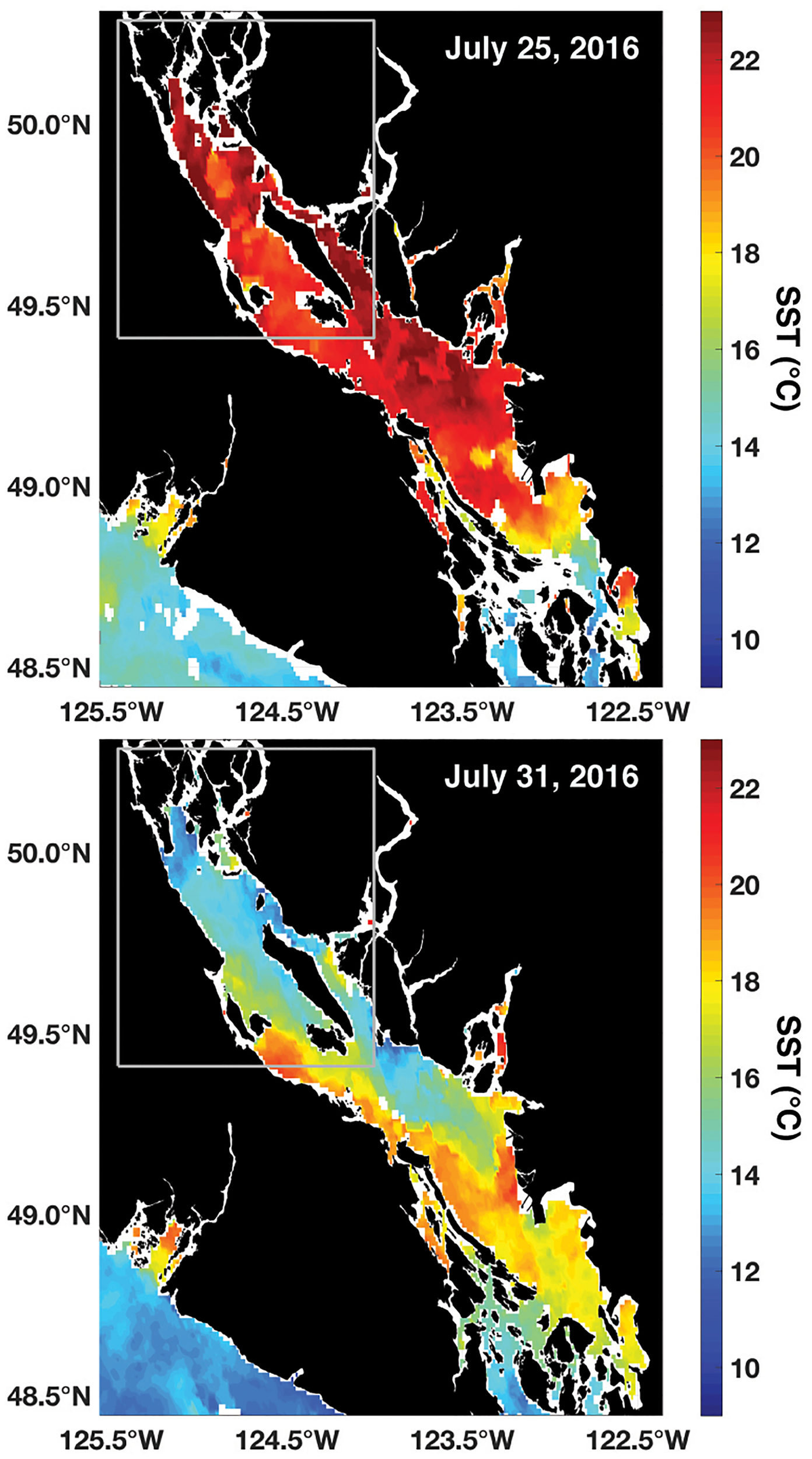
Figure 6. NOAA Polar Operational Environmental Satellite (POES) Advanced Very High Resolution Radiometer (AVHRR) daily average (night and day passes) 1.1 km SST (°C) at the start (top) and peak (bottom) of the July 2016 high-CO₂ event. The gray box marks the NSS as outlined in Figure 1.

Large summer wind-driven variability did not occur each year in the NSS, and this may have far-reaching ecosystem-level implications. For instance, following the 2016 wind event, super-saturated dissolved oxygen levels >60 μmol kg^-1 were observed beginning ∼1 week after the maximum in seawater pCO₂ (Supplementary Figure S4). In addition, the trajectory of SST, salinity, and pCO₂ over the 4 days following the occurrence of maximal seawater pCO₂ during the 2016 event suggests a strong biological response (Figure 5). At buoy 46131 during this interval, salinity was stable while SST warmed by ∼3°C. Driven by solubility alone, this warming should have increased pCO₂ by ∼80 μatm. However, seawater pCO₂ decreased over the 4 days from 700 to 200 μatm. Sea-air CO₂ exchange alone cannot explain this precipitous drop in pCO₂ to undersaturated levels with respect to the atmosphere. Even with a sustained maximal sea-air CO₂ exchange of ∼1 mmol m^-2 hr^-1 (data not shown but observed during the 2016 event), it would take >200 days to equilibrate a 20 m surface layer with the SST, salinity, and pCO₂ levels observed during the event. These biogeochemical lines of evidence suggest a strong primary productivity response to wind-driven high-CO₂ events in the NSS. While this variability may stimulate productivity, with potentially food web implications, it also means short-term exposure to adverse conditions for marine life vulnerable to low-Ω_arag and low-pH_T (Waldbusser and Salisbury, 2014; McLaskey et al., 2016; Bednarsek et al., 2017).

The Lack of High-CO₂ Summertime Conditions in 2017

Important NSS interannual variability was revealed by the lack of high-CO₂ summertime conditions in 2017 that had been observed in 2015 and 2016 associated with strong northwesterly wind events. The drivers of this variability at the regional scale can be assessed by examining the rate of energy transfer from the winds to the surface ocean (Denman and Miyake, 1973) and how this input compares to the potential energy needed to mix the upper water column (Hauri et al., 2013), which is related to the stratification (Supplementary Text 2). The significance of a single summertime wind event equates to the integrated rate of energy transfer over the duration of the event, with an event defined here as wind conditions over 5 m s^-1 that resulted in energy transfer ≥0.19 mJ m^-2 s^-1 at a mean drag coefficient of 0.00128 and an air density of 1.22 kg m^-3. High-CO₂ events in 2015 and 2016 (Supplementary Figures S1, S2 and Figures 5, 6) were each associated with instances where energy from the winds overcame upper ocean stratification (Figure 7), however, these conditions did not occur in 2017. In 2017, wind strength was inadequate to overcome the nearly 50% higher potential energy requirement needed to mix the upper 20 m. While weaker winds in 2017 clearly played a role in not forcing high-CO₂, the energy needed to mix the upper water column, and hence the stratification, was significantly higher (Figure 7). Greater freshwater content in the NSS during 2017 (Figure 8), calculated following the relationship from Proshutinsky et al. (2009), increased the energy needed to mix the surface water column (Figure 7) and halted any potential influence from the weaker winds to drive high-CO₂ conditions. Given that El Niño winters in BC are typically warmer and drier (Shabbar et al., 1997), and that 2015 and 2016 were both warm years, we speculate that there may be a relationship whereby El Niño winters set the stage for reduced freshwater content in the NSS during summer, enabling the upper water column to be more easily mixed by northwesterly winds. Although only tenuously supported by the 3.5 years of data presented here, the growing QIFS dataset will help to further elucidate this potential pattern on summertime surface CO₂ variability.

FIGURE 7

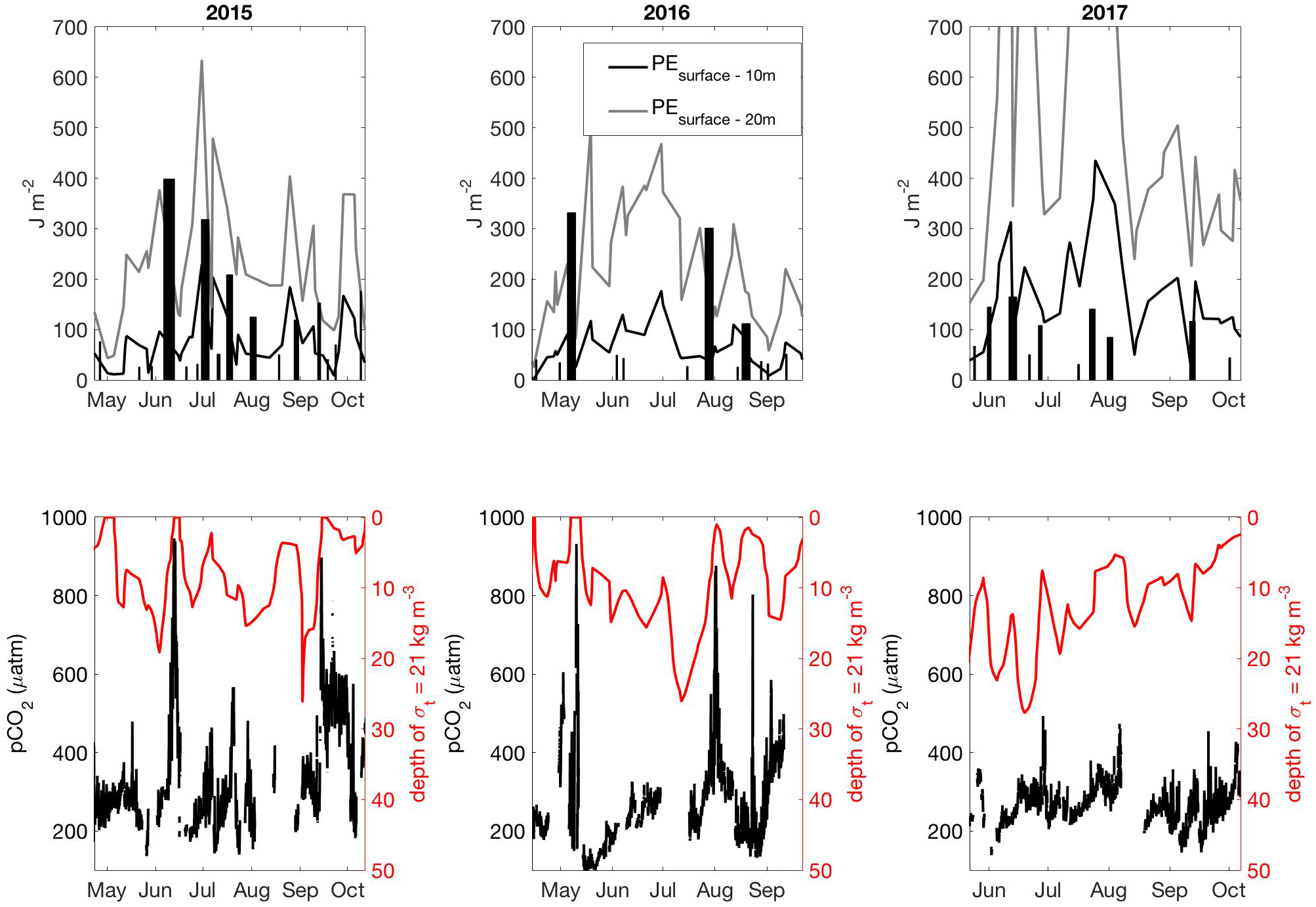
Figure 7. Top row is the integrated rate of energy transfer (J m^-2; bars) over the duration of wind events observed between the spring and fall transitions (Supplementary Figure S5) in 2015 (left), 2016 (middle), and 2017 (right). The width of the bars equates to the duration of the wind event. The top panels also show the potential energy needed to mix the upper water column (surface to 10 m in black, surface to 20 m in gray). Lower panel is surface water pCO₂ from QIFS (black) and the depth of the 21 kg m^-3 density anomaly (σ_t) surface.

FIGURE 8

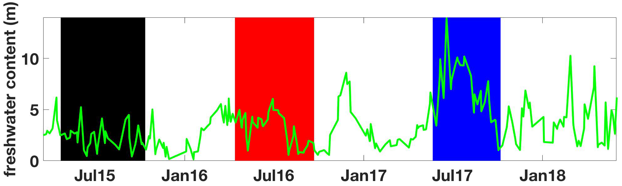
Figure 8. Freshwater content at QU39 from March 18, 2015 to June 1, 2018 computed using a reference salinity of 29.1 following the relationship from Proshutinsky et al. (2009). Vertical shaded areas mark the time periods between spring and fall transitions color-coded to match the years shown in Supplementary Figures S5, S6.

Crossing CO₂ System Thresholds in the NSS

The variability of surface NSS CO₂ parameters was maximal during summer, and year-to-year differences in the drivers of summertime variability were important and linked to the combined influences of northwesterly wind events and freshwater content, as shown above. Increasing anthropogenic CO₂ content (Supplementary Figure S3) under the “business as usual” scenario will shift the system further to less favorable conditions for marine life sensitive to low-Ω_arag and/or low-pH_T exposure. Using TCO₂ estimated for each year in the anthropogenic CO₂ calculation, we derived Ω_arag and pH_T for NSS surface water spanning 1765 to the end of the 21st century (Figure 9). As mentioned above, the calculation is based on data from 2017; therefore the seasonal dynamics are slightly biased toward less variable Ω_arag and pH_T conditions due to the lack of observed summertime wind-driven vertical mixing that year (Figure 4). Nonetheless, our analysis shows that NSS surface water was consistently above the thermodynamic threshold of Ω_arag = 1 at the start of the Industrial Revolution. Observed wintertime surface water Ω_arag < 1 (Figure 4) was shown to have developed only over the last century (Figure 9); a change that has occurred simultaneously with the development of C. gigas culture in BC beginning in ∼1900 (Quayle, 1988).

FIGURE 9

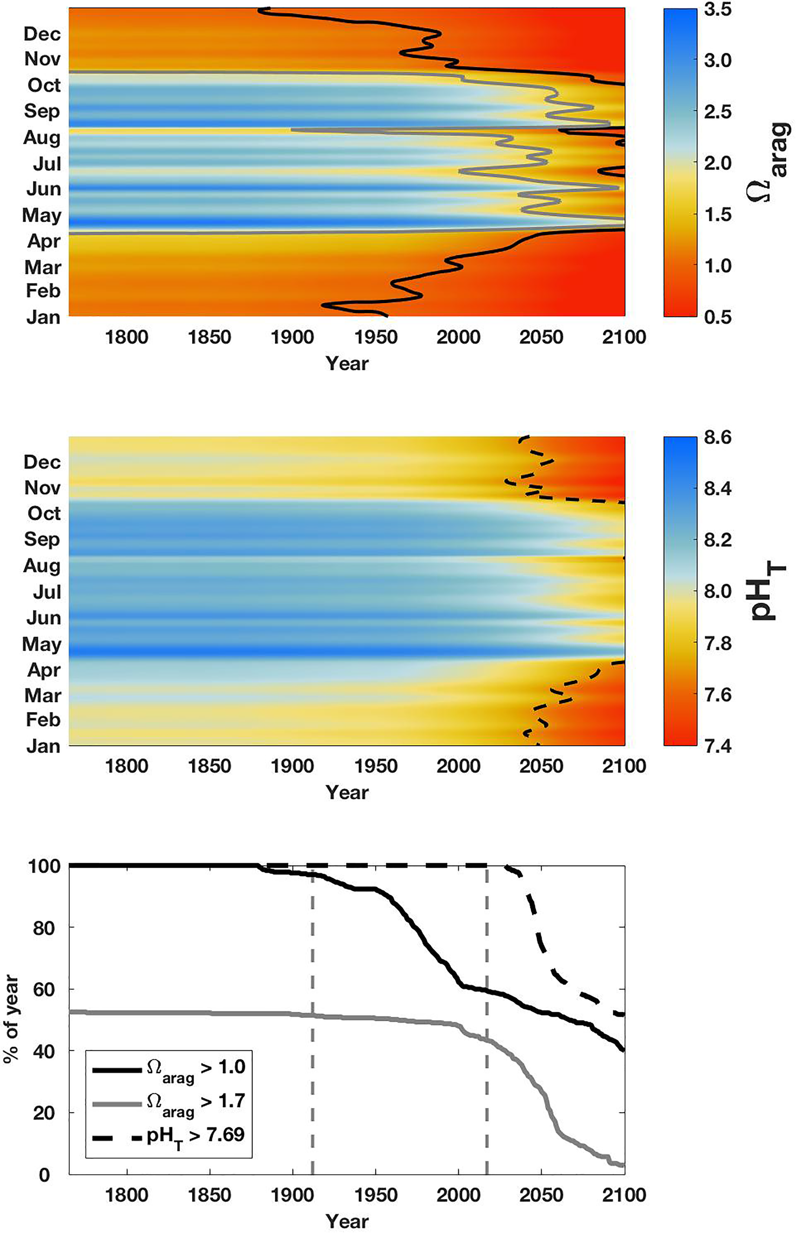
Figure 9. Projections from 1765 to 2100 of surface water Ω_arag (top), pH_T (middle), and the percent of the year with values above key thresholds (bottom): Ω_arag = 1 (black), Ω_arag = 1.7 (gray), and pH_T = 7.69 (dashed black). These thresholds are highlighted in the upper panels. 2017 QIFS data used in these projections were smoothed using a 14-day LOESS filter.

Surface conditions during winter may have always been below the “break-even” point for larval biomass production of Ω_arag = 1.7 (Figure 9), as well as near levels shown experimentally to induce stress in the larvae of C. gigas, M. galloprovincialis, and M. californianus larvae (Waldbusser et al., 2014, 2015). It should be noted that winter periods are generally typified by the absence of larvae and reduced adult shellfish growth (Gosling, 2003). However, crossing the thermodynamic threshold in winter marks the shift toward a seasonal full water column corrosive environment. Spring CO₂ drawdown, which initiates with variable timing, establishes a refugia only in the surface layer that can be disrupted by episodic forcing and then subsequently breaks down in autumn. The biological implications of this contemporary window of non-corrosive conditions are unknown and require immediate further study, albeit point to a reduction in suitable habitat for vulnerable resident prey species (i.e., L. helicina; Bednarsek et al., 2014) and reduced calcification (Kroeker et al., 2013) with potential implications for shell-forming populations.

The shift in winter Ω_arag conditions was shown in our assessment to cross the thermodynamic Ω_arag threshold earlier than the shift in pH_T to levels low enough to potentially slow E. pacifica larval development (McLaskey et al., 2016). Beginning in 2030, the percent of the year above pH_T = 7.69 rapidly decreases (Figure 9), representing the onset of surface conditions that may impact E. pacifica larvae. This increased pressure on E. pacifica survival could subsequently lead to indirect ecosystem effects by way of reducing an important prey item for many species of salmon in the study area (Brodeur et al., 2007). Near the same time as when winter pH_T conditions drop below this threshold for E. pacifica, summertime Ω_arag values above 1.7 also rapidly decline, marking a transition to perennially stressful levels for vulnerable larval shellfish species with potential impacts for population stability and ecosystem structure.

Limitations of Long-Term Assessment

Our estimation of changing NSS surface water Ω_arag and pH_T shows the time scales over which thermodynamic and biological thresholds will be crossed (Figure 9). However, cautionary notes must be made. First, our analysis utilized the “business as usual” emissions trajectory, and would over-estimate shifting Ω_arag and pH_T conditions over the remainder of the century if global CO₂ emissions decrease. Second, the calculations assumed consistency in SST, salinity, and Alk_inorganic variance. In coastal settings, this assumption can be violated, such as seen in the Gulf of Maine (Salisbury and Jönsson, 2018) and Baltic Sea (Müller et al., 2016). While warming in Strait of Georgia surface water has been estimated to be ∼1°C century^-1 (Riche et al., 2014), which would have a ∼1% impact on projected Ω_arag and pH_T, unaccounted for variance in salinity and Alk_inorganic is an unknown and requires further investigation. For comparison, the observed alkalinity increase in the central Baltic Sea compensated CO₂-induced acidification by almost 50% and stabilized Ω_arag over a 2-decade period (Müller et al., 2016). Third, our approach assumed constant seasonality in ΔTCO_2,diseq; an assumption that could be prone to failure in the presence of increasing eutrophication. Fourth, while experimental work has identified some Ω_arag and pH_T thresholds, the combined impact of the projected chemical changes with additional environmental stressors, such as warming, hypoxia, marine pollutants, will be an important determinant for adaptive capacity. The ability for vulnerable marine organisms to adapt will be a function of the rate of environmental change, population plasticity, and genetic selection processes (Sunday et al., 2014). Adaptive capacity will ultimately determine whether the passage of experimentally determined biological Ω_arag and pH_T thresholds negatively impacts vulnerable organisms and the ecosystems they reside in.

Author Contributions

WE, KP, AH, and CW carried out all CO₂ data collection presented in this study. BH provided guidance on analytical system operation. WE and BH established data handling protocols. WE, JJ, and AH analyzed interannual variability in NSS surface CO₂. WE and HG-S initially developed CO₂ observing at QIFS. JM provided the instrumentation as well as the SeaFET used on Environment Canada buoy 46131. WE, SA, and RF conducted data collection from NOAA WCOA2016. WE wrote the manuscript. All authors provided input to the text.

Funding

This work was provided by the Tula Foundation, with some instruments and ship-time provided by partnering agencies including the National Oceanic and Atmospheric Administration.

Conflict of Interest Statement

The authors declare that the research was conducted in the absence of any commercial or financial relationships that could be construed as a potential conflict of interest.

Acknowledgments

We would like to acknowledge that this study occurred within the traditional territories of the Heiltsuk, the Wuikinuxv, the Kwakwaka’wakw, and the Coast Salish peoples. We would like to thank the numerous citizen scientists, Vancouver Island University Deep Bay Marine Field Station staff, and Hakai Institute field technicians who collected many of the seawater samples and CTD data used in this study. We would also like to thank the Pacific Salmon Foundation and Environment Canada for the opportunity to deploy instrumentation on weather buoy 46131. We thank the captain and crew of the NOAA ship Ronald H. Brown used during WCOA2016. We are extremely appreciative of the Tula Foundation for supporting the research presented here. SA and RF thank the NOAA Ocean Acidification Program for their support of this research. We would like to thank two reviewers for their valued and constructive comments that helped to improve this manuscript. Contribution number 4849 from the Pacific Marine Environmental Laboratory of NOAA.

Supplementary Material

The Supplementary Material for this article can be found online at: https://www.frontiersin.org/articles/10.3389/fmars.2018.00536/full#supplementary-material

Footnotes

1. ^http://dx.doi.org/10.21966/1.521066

References

Bakri, T., Jackson, P., and Doherty, F. (2017). A synoptic climatology of strong along-channel winds on the Coast of British Columbia. Canada. Int. J. Climatol. 37, 2398–2412. doi: 10.1002/joc.4853

CrossRef Full Text | Google Scholar

Bandstra, L., Hales, B., and Takahashi, T. (2006). High-frequency measurements of total CO2: method development and first oceanographic observations. Mar. Chem. 100, 24–38. doi: 10.1016/j.marchem.2005.10.009

CrossRef Full Text | Google Scholar

Barton, A., Hales, B., Waldbusser, G., Langdon, C., and Feely, R. A. (2012). The Pacific oyster, Crassostrea gigas, shows negative correlation to naturally elevated carbon dioxide levels: implications for near-term ocean acidification effects. Limnol. Oceanogr. 57, 698–710. doi: 10.4319/lo.2012.57.3.0698

CrossRef Full Text | Google Scholar

Barton, A., Waldbusser, G. G., Feely, R. A., Weisberg, S. B., Newton, J. A., Hales, B., et al. (2015). Impacts of coastal acidification on the Pacific Northwest shellfish industry and adaptation strategies implemented in response. Oceanography 28, 146–159. doi: 10.5670/oceanog.2015.38

CrossRef Full Text | Google Scholar

Bednarsek, N., Feely, R. A., Reum, J. C., Peterson, B., Menkel, J., Alin, S. R., et al. (2014). Limacina helicina shell dissolution as an indicator of declining habitat suitability owing to ocean acidification in the California Current Ecosystem. Proc. Biol. Sci. 281:20140123. doi: 10.1098/rspb.2014.0123

PubMed Abstract | CrossRef Full Text | Google Scholar

Bednarsek, N., Feely, R. A., Tolimieri, N., Hermann, A. J., Siedlecki, S. A., Waldbusser, G. G., et al. (2017). Exposure history determines pteropod vulnerability to ocean acidification along the US West Coast. Sci. Rep. 7:4526. doi: 10.1038/s41598-41017-03934-z

PubMed Abstract | CrossRef Full Text | Google Scholar

Bianucci, L., Long, W., Khangaonkar, T., Pelletier, G., Ahmed, A., Mohamedali, T., et al. (2018). Sensitivity of the regional ocean acidification and carbonate system in Puget Sound to ocean and freshwater inputs. Elem. Sci. Anth. 6:22. doi: 10.1525/elementa.151

CrossRef Full Text | Google Scholar

Brodeur, R., Daly, E. A., Sturdevant, M. V., Miller, T. W., Moss, J. H., Thiess, M. E., et al. (2007). Regional comparisons of juvenile salmon feeding in coastal Marine waters off the West Coast of North America. Am. Fish. Soc. Symp. 57, 183–203.

Google Scholar

Caldeira, K., and Wickett, M. E. (2003). Anthropogenic carbon and ocean pH. Nature 425:365. doi: 10.1038/425365a

PubMed Abstract | CrossRef Full Text | Google Scholar

Chan, F., Barth, J. A., Blanchette, C. A., Byrne, R. H., Chavez, F. P., Cheriton, O., et al. (2017). Persistent spatial structuring of coastal ocean acidification in the California Current System. Sci. Rep. 7:2526. doi: 10.1038/s41598-41017-02777-y

PubMed Abstract | CrossRef Full Text | Google Scholar

Cooley, S. R., and Doney, S. C. (2009). Anticipating ocean acidification’s economic consequences for commercial fisheries. Environ. Res. Lett. 4, 1–8. doi: 10.1088/1748-9326/1084/1082/024007

PubMed Abstract | CrossRef Full Text | Google Scholar

Cooley, S. R., Kite-Powell, H. L., and Doney, S. C. (2009). Ocean acidification’s potential to alter global marine ecosystem services. Oceanography 22, 172–181. doi: 10.5670/oceanog.2009.106

CrossRef Full Text | Google Scholar

Denman, K. L., and Miyake, M. (1973). Behavior of the mean wind, the drag coefficient, and the wave field in the open ocean. J. Geophyis. Res. 78, 1917–1931. doi: 10.1029/JC078i012p01917

CrossRef Full Text

Dickson, A., Wesolowski, D. J., Palmer, D. A., and Mesmer, R. E. (1990). Dissociation constant of bisulfate ion in aqueous sodium chloride solutions to 250 °C. J. Phys. Chem. 94, 7978–7985. doi: 10.1021/j100383a042

CrossRef Full Text | Google Scholar

Doney, S. C., Ruckelshaus, M., Duffy, J. E., Barry, J. P., Chan, F., English, C. A., et al. (2012). Climate change impacts on marine ecosystems. Ann. Rev. Mar. Sci. 4, 11–37. doi: 10.1146/annurev-marine-041911-111611

PubMed Abstract | CrossRef Full Text | Google Scholar

Egleston, E. S., Sabine, C. L., and Morel, F. M. M. (2010). Revelle revisited: buffer factors that quantify the response of ocean chemistry to changes in DIC and alkalinity. Glob. Biogeochem. Cycles 24:GB1002. doi: 10.1029/2008GB003407

CrossRef Full Text | Google Scholar

Ekstrom, J. A., Suatoni, L., Cooley, S. R., Pendleton, L. H., Waldbusser, G. G., Cinner, J. E., et al. (2015). Vulnerability and adaptation of US shellfisheries to ocean acidification. Nat. Clim. Chang. 5, 207–214. doi: 10.1038/nclimate2508

CrossRef Full Text | Google Scholar

Evans, W., Hales, B., Strutton, P. G., and Ianson, D. (2012). Sea-air CO2 fluxes in the western Canadian coastal ocean. Prog. Oceanogr. 101, 78–91. doi: 10.1016/j.pocean.2012.1001.1003

CrossRef Full Text | Google Scholar

Evans, W., Mathis, J. T., Ramsay, J., and Hetrick, J. (2015). On the frontline: tracking ocean acidification in an alaskan shellfish hatchery. PLoS One 10:e0130384. doi: 10.1371/journal.pone.0130384

PubMed Abstract | CrossRef Full Text | Google Scholar

Fassbender, A. J., Alin, S. R., Feely, R. A., Sutton, A. J., Newton, J., Krembs, C., et al. (2018). Seasonal carbonate chemistry variability in marine surface waters of the Pacific Northwest. Earth Syst. Sci. Data 10, 1367–1401. doi: 10.1371/journal.pone.0089619

PubMed Abstract | CrossRef Full Text | Google Scholar

Fassbender, A. J., Alin, S. R., Feely, R. A., Sutton, A. J., Newton, J. A., and Byrne, R. H. (2016). Estimating total alkalinity in the washington state coastal zone: complexities and surprising utility for ocean acidification research. Estuaries Coasts 40, 404–418. doi: 10.1007/s12237-12016-10168-z

CrossRef Full Text | Google Scholar

Feely, R. A., Alin, S. R., Carter, B., Bednarsek, N., Hales, B., Chan, F., et al. (2016). Chemical and biological impacts of ocean acidification along the west coast of North America. Estuarine Coastal Shelf Sci. 183, 260–270. doi: 10.1016/j.ecss.2016.08.043

CrossRef Full Text | Google Scholar

Feely, R. A., Alin, S. R., Newton, J., Sabine, C. L., Warner, M., Devol, A., et al. (2010). The combined effects of ocean acidification, mixing, and respiration on pH and carbonate saturation in an urbanized estuary. Estuarine Coastal Shelf Sci. 88, 442–449. doi: 10.1016/j.ecss.2010.05.004

CrossRef Full Text | Google Scholar

Feely, R. A., Okazaki, R. R., Cai, W. J., Bednarsek, N., Alin, S. R., Byrne, R. H., et al. (2018). The combined effects of acidification and hypoxia on pH and aragonite saturation in the coastal waters of the California current ecosystem and the northern Gulf of Mexico. Cont. Shelf Res. 152, 50–60. doi: 10.1016/j.csr.2017.11.002

CrossRef Full Text | Google Scholar

Feely, R. A., Sabine, C. L., Lee, K., Berelson, W., Kleypas, J., Fabry, V. J., et al. (2004). Impact of anthropogenic CO₂ on the CaCO₃ System in the oceans. Science 305, 362–366. doi: 10.1126/science.1097329

PubMed Abstract | CrossRef Full Text | Google Scholar

Gosling, E. (2003). Bivalve Molluscs: Biology, Ecoogy and Culture. Malden, MA: Blackwell Publishing, Inc. doi: 10.1002/9780470995532

CrossRef Full Text | Google Scholar

Haigh, R., Ianson, D., Holt, C. A., Neate, H. E., and Edwards, A. M. (2015). Effects of ocean acidification on temperature coastal marine ecosystems and fisheries in the Northeast Pacific. PLoS One 10:e0117533. doi: 10.1371/journal.pone.0117533

PubMed Abstract | CrossRef Full Text | Google Scholar

Hales, B., Chipman, D., and Takahashi, T. (2004). High-frequency measurements of partial pressure and total concentration of carbon dioxide in seawater using microporous hydrophobic membrane contactors. Limnol. Oceanogr. 2, 356–364. doi: 10.4319/lom.2004.2.356

CrossRef Full Text

Hales, B., Suhrbier, A., Waldbusser, G. G., Feely, R. A., and Newton, J. A. (2016). The carbonate chemistry of the “Fattening Line,” Willapa Bay, 2011-2014. Estuaries Coasts 40, 173–186. doi: 10.1007/s12237-12016-10136-12237

CrossRef Full Text | Google Scholar

Hales, B., Takahashi, T., and Bandstra, L. (2005). Atmospheric CO2 uptake by a coastal upwelling system. Glob. Biogeochem. Cycles 19:GB1009. doi: 10.1029/2004GB002295

CrossRef Full Text | Google Scholar

Harris, K. E., Degrandpre, M. D., and Hales, B. (2013). Aragonite saturation state dynamics in a coastal upwelling zone. Geophys. Res. Lett. 40, 2720–2725. doi: 10.1002/grl.50460

CrossRef Full Text | Google Scholar

Hauri, C., Winsor, P., Juranek, L. W., Mcdonnell, A. M. P., Takahashi, T., and Mathis, J. T. (2013). Wind-driven mixing causes a reduction in the strength of the continental shelf carbon pump in the Chukchi Sea. Geophys. Res. Lett. 40, 5932–5936. doi: 10.1002/2013GL058267

CrossRef Full Text | Google Scholar

Hsu, S. A., Meindl, E. A., and Gilhousen, D. B. (1994). Determining the power-law wind-profile exponent under near-neutral stability conditions at sea. J. Appl. Meteorol. 33, 757–765. doi: 10.1175/1520-0450(1994)033<0757:DTPLWP>2.0.CO;2

CrossRef Full Text

Ianson, D., Allen, S. E., Moore-Maley, B. L., Johannessen, S. C., and Macdonald, R. W. (2016). Vulnerability of a semienclosed estuarine sea to ocean acidification in contrast with hypoxia. Geophys. Res. Lett. 43, 5793–5801. doi: 10.1002/2016GL068996

CrossRef Full Text | Google Scholar

Johannessen, S. C., Masson, D., and Macdonald, R. W. (2014). Oxygen in the deep strait of Georgia, 1951-2009: the roles of mixing, deep-water renewal, and remineralization of organic carbon. Limnol. Oceanogr. 59, 211–222. doi: 10.4319/lo.2014.59.1.0211

CrossRef Full Text | Google Scholar

Journey, M. L., Trudel, M., Young, G., and Beckman, B. R. (2018). Evidence of depressed growth of juvenile Pacific salmon (Oncorhynchus) in Johnstone and Queen Charlotte Straits, British Columbia. Fish. Oceanogr. 27, 174–183. doi: 10.1111/fog.12243

CrossRef Full Text | Google Scholar

Kroeker, K. J., Kordas, R. L., Crim, R., Hendriks, I. E., Ramajo, L., Singh, G. S., et al. (2013). Impacts of ocean acidification on marine organisms: quantifying sensitivities and interactions with warming. Glob. Chang. Biol. 19, 1884–1896. doi: 10.1111/gcb.12179

PubMed Abstract | CrossRef Full Text | Google Scholar

Landschützer, P., Gruber, N., Bakker, D. C. E., Stemmler, I., and Six, K. D. (2018). Strengthening seasonal marine CO2 variations due to increasing atmospheric CO2. Nat. Clim. Chang. 8, 146–150. doi: 10.1038/s41558-41017-40057-x

CrossRef Full Text | Google Scholar

Laruelle, G. G., Cai, W. J., Hu, X., Gruber, N., Mackenzie, F. T., and Regnier, P. (2018). Continental shelves as a variable but increasing global sink for atmospheric carbon dioxide. Nat. Commun. 9:454. doi: 10.1038/s41467-41017-02738-z

PubMed Abstract | CrossRef Full Text

Lueker, T. J., Dickson, A. G., and Keeling, C. D. (2000). Ocean pCO2 calculated from dissolved inorganic carbon, alkalinity, and equations for K1 and K2: validation based on laboratory measurements of CO2 in gas and seawater at equilibrium. Mar. Chem. 70, 105–119. doi: 10.1016/S0304-4203(00)00022-0

CrossRef Full Text | Google Scholar

Masson, D. (2002). Deep water renewal in the strait of Georgia. Estuarine Coastal Shelf Sci. 54, 115–126. doi: 10.1006/ecss.2001.0833

CrossRef Full Text | Google Scholar

Masson, D., and Cummins, P. F. (2004). Observations and modeling of seasonal variability in the straits of Georgia and Juan de Fuca. J. Mar. Res. 62, 491–516. doi: 10.1357/0022240041850075

CrossRef Full Text | Google Scholar

Masson, D., and Peña, A. (2009). Chlorophyll distribution in a temperature estuary: the strait of Georgia and Juan de Fuca Striat. Estuarine Coastal Shelf Sci. 82, 19–28. doi: 10.1016/j.ecss.2008.12.022

CrossRef Full Text | Google Scholar

Mathis, J. T., Cooley, S. R., Lucey, N., Colt, S., Ekstrom, J., Hurst, T., et al. (2015). Ocean acidification risk assessment for Alaska’s fishery sector. Prog. Oceanogr. 136, 71–91. doi: 10.1016/j.pocean.2014.07.001

CrossRef Full Text | Google Scholar

McLaskey, A. K., Keister, J. E., Mcelhany, P., Brady Olson, M., Busch, D. S., Maher, M., et al. (2016). Development of Euphausia pacifica (krill) larvae is impaired under pCO2 levels currently observed in the Northeast Pacific. Mar. Ecol. Prog. Ser. 555, 65–78. doi: 10.3354/meps11839

CrossRef Full Text | Google Scholar

McLaughlin, K., Weisberg, S., Dickson, A., Hofmann, G., Newton, J., Aseltine-Neilson, D., et al. (2015). Core principles of the california current acidification network: linking chemistry, physics, and ecological effects. Oceanography 25, 160–169. doi: 10.5670/oceanog.2015.39

CrossRef Full Text | Google Scholar

Moore-Maley, B. L., Allen, S. E., and Ianson, D. (2016). Locally driven interannual variability of near-surface pH and ΩA in the strait of Georgia. J. Geophys. Res. 121, 1600–1625. doi: 10.1002/2015JC011118

CrossRef Full Text | Google Scholar

Mucci, A. (1983). The solubility of calcite and aragonite in seawater at various salinities, temperatures, and one atmosphere total pressure. Am. J. Sci. 283, 780–799. doi: 10.2475/ajs.283.7.780

CrossRef Full Text | Google Scholar

Müller, J. D., Schneider, B., and Rehder, G. (2016). Long-term alkalinity trends in the Baltic Sea and their implications for CO2-induced acidification. Limnol. Oceanogr. 61, 1984–2002. doi: 10.1002/lno.10349

CrossRef Full Text | Google Scholar

Newton, J. A., Feely, R. A., Jewett, E. B., Williamson, P., and Mathis, J. (2015). Global Ocean Acidification Observing Network: Requirements and Governance Plan. Available at: http://goa-on.org/documents/resources/GOA-ON_2nd_edition_final.pdf

Google Scholar

Orr, J. C., Epitalon, J.-M., Dickson, A. G., and Gattuso, J.-P. (2018). Routine uncertainty propagation for the marine carbon dioxide system. Mar. Chem. 207, 84–107. doi: 10.1016/j.marchem.2018.10.006

CrossRef Full Text | Google Scholar

Orr, J. C., Fabry, V. J., Aumont, O., Bopp, L., Doney, S. C., Feely, R. A., et al. (2005). Anthropogenic ocean acidification over the twenty-first century and its impact on calcifying organisms. Nature 437, 681–686. doi: 10.1038/nature04095

PubMed Abstract | CrossRef Full Text | Google Scholar

Pacella, S. R., Brown, C. A., Waldbusser, G. G., Labiosa, R. G., and Hales, B. (2018). Seagrass habitat metabolism increases short-term extremes and long-term offset of CO2 under future ocean acidification. Proc. Natl. Acad. Sci. U.S.A. 115, 3870–3875. doi: 10.1073/pnas.1703445115

PubMed Abstract | CrossRef Full Text | Google Scholar

Pawlowicz, R., Riche, O., and Halverson, M. (2007). The circulation and residence time of the strait of georgia using a simple mixing-box approach. Atmos. Ocean 45, 173–193. doi: 10.3137/ao.450401

CrossRef Full Text | Google Scholar

Pierrot, D., Neill, C., Sullivan, K., Castle, R., Wanninkhof, R., Lüger, H., et al. (2009). Recommendations for autonomous underway pCO2 measuring systems and data-reduction routines. Deep Sea Res. II 56, 512–522. doi: 10.1016/j.dsr2.2008.12.005

CrossRef Full Text | Google Scholar

Proshutinsky, A., Krishfield, R., Timmermans, M.-L., Toole, J., Carmack, E., Mclaughlin, F., et al. (2009). Beaufort Gyre freshwater reservoir: state and variability from observations. J. Geophyis. Res. 114:C00A10. doi: 10.1029/2008JC005104

CrossRef Full Text | Google Scholar

Quayle, D. B. (1988). “Pacific oyster culture in British Columbia,” in Canadian Bulletin of Fisheries and Aquatic Sciences 218, ed. Department of Fisheries and Oceans (Ottawa, ON: Department of Fisheries and Oceans).

Google Scholar

Riahi, K., Rao, S., Krey, V., Cho, C., Chirkov, V., Fischer, G., et al. (2011). RCP 8.5 – A scenario of comparatively high greenhouse gas emissions. Clim. Chang. 109, 33–57. doi: 10.1007/s10584-011-0149-y

CrossRef Full Text | Google Scholar

Riche, O., Johannessen, S. C., and Macdonald, R. W. (2014). Why timing matters in a coastal sea: trends, variability and tipping points in the Strait of Georgia, Canada. J. Mar. Syst. 131, 36–53. doi: 10.1016/j.jmarsys.2013.11.003

CrossRef Full Text | Google Scholar

Sabine, C. L., Feely, R. A., Gruber, N., Key, R. M., Lee, K., Bullister, J. L., et al. (2004). The oceanic sink for anthropogenic CO2. Science 305, 367–371. doi: 10.1126/science.1097403

PubMed Abstract | CrossRef Full Text | Google Scholar

Sabine, C. L., Feely, R. A., Key, R. M., Bullister, J. L., Millero, F. J., Lee, K., et al. (2002). Distribution of anthropogenic CO2 in the Pacific Ocean. Glob. Biogeochem. Cycles 16, 30–31. doi: 10.1029/2001GB001639

CrossRef Full Text | Google Scholar

Salisbury, J. E., and Jönsson, B. F. (2018). Rapid warming and salinity changes in the Gulf of Maine alter surface ocean carbonate parameters and hide ocean acidification. Biogeochemistry 141, 401–418. doi: 10.1007/s10533-018-0505-3

CrossRef Full Text | Google Scholar

Seung, C. K., Dalton, M. G., Punt, A. E., Poljak, D., and Foy, R. (2015). Economic impacts of changes in an alaska crab fishery from ocean acidification. Clim. Chang. Econ. 6:1550017. doi: 10.1142/S2010007815500177

CrossRef Full Text | Google Scholar

Shabbar, A., Bonsal, B., and Khandekar, M. (1997). Canadian precipitation patterns associated with the southern oscillation. J. Clim. 10, 3016–3027. doi: 10.1175/1520-0442(1997)010<3016:CPPAWT>2.0.CO;2

CrossRef Full Text

Smith, S. D., Anderson, R. J., Oost, W. A., Kraan, C., Maat, N., Decosmo, J., et al. (1991). Sea surface wind stress and drag coefficients: the HEXOS results. Boundary-Layer Meteorology 60, 109–142. doi: 10.1007/BF00122064

CrossRef Full Text | Google Scholar

Sunday, J. M., Calosi, P., Dupont, S., Munday, P. L., Stillman, J. H., and Reusch, T. B. (2014). Evolution in an acidifying ocean. Trends Ecol. Evol. 29, 117–125. doi: 10.1016/j.tree.2013.11.001

PubMed Abstract | CrossRef Full Text | Google Scholar

Sutton, A. J., Feely, R. A., Maenner-Jones, S., Musielewicz, S., Osborne, J., Dietrich, C., et al. (2018). Autonomous seawater pCO2 and pH time series from 40 surface buoys and the emergence of anthropogenic trends. Earth Syst. Sci. Data Discuss. doi: 10.5194/essd-2018-5177

CrossRef Full Text | Google Scholar

Sutton, A. J., Sabine, C. L., Feely, R. A., Cai, W. J., Cronin, M. F., Mcphaden, M. J., et al. (2016). Using present-day observations to detect when anthropogenic change forces surface ocean carbonate chemistry outside preindustrial bounds. Biogeosciences 13, 5065–5083. doi: 10.5194/bg-13-5065-2016

CrossRef Full Text | Google Scholar

Takahashi, T. (1961). Carbon dioxide in the atmosphere and in atlantic ocean water. J. Geophyis. Res. 66, 477–494. doi: 10.1029/JZ066i002p00477

CrossRef Full Text | Google Scholar

Takeshita, Y., Frieder, C. A., Martz, T. R., Ballard, J. R., Feely, R. A., Kram, S., et al. (2015). Including high-frequency variability in coastal ocean acidification projections. Biogeosciences 12, 5853–5870. doi: 10.1371/journal.pone.0085117

PubMed Abstract | CrossRef Full Text | Google Scholar

Tortell, P. D., Merzouk, A., Ianson, D., Pawlowicz, R., and Yelland, D. R. (2012). Influence of regional climate forcing on surface water pCO2, ΔO2/Ar and dimethylsulfide (DMS) along the southern British Columbia coast. Cont. Shelf Res. 47, 119–132. doi: 10.1016/j.csr.2012.07.007

CrossRef Full Text | Google Scholar

Uppström, L. R. (1974). The boron/chlorinity ratio of deep-sea water from the pacific ocean. Deep Sea Res. Oceanogr. Abstracts 21, 161–162. doi: 10.1016/0011-7471(74)90074-6

CrossRef Full Text | Google Scholar

Van Heuven, S., Pierrot, D., Rae, J. W. B., Lewis, E., and Wallace, D. W. R. (2011). “MATLAB program developed for CO₂ system calculations,” in ORNL/CDIAC-105b, ed. Carbon Dioxide Information Analysis Center (Oak Ridge, TN: Department of Energy).

Google Scholar

Voss, B. M., Peucker-Ehrenbrink, B., Eglinton, T. I., Fiske, G., Wang, Z. A., Hoering, K. A., et al. (2014). Tracing river chemistry in space and time: dissolved inorganic constituents of the Fraser River. Canada. Geochim. Cosmochim. Acta 124, 283–308. doi: 10.1016/j.gca.2013.09.006

CrossRef Full Text | Google Scholar

Waldbusser, G. G., Hales, B., Langdon, C., Haley, B. A., Schrader, P., Brunner, E. L., et al. (2015). Ocean acidification has multiple modes of action on bivalve larvae. PLoS One 10:e0128376. doi: 10.1371/journal.pone.0128376

PubMed Abstract | CrossRef Full Text | Google Scholar

Waldbusser, G. G., Hales, B., Langdon, C. J., Haley, B. A., Schrader, P., Brunner, E. L., et al. (2014). Saturation-state sensitivity of marine bivalve larvae to ocean acidification. Nat. Clim. Chang. 5, 273–280. doi: 10.1038/nclimate2479

CrossRef Full Text | Google Scholar

Waldbusser, G. G., and Salisbury, J. E. (2014). Ocean acidification in the coastal zone from an organism’s perspective: multiple system parameters, frequency domains, and habitats. Ann. Rev. Mar. Sci. 6, 221–247. doi: 10.1146/annurev-marine-121211-172238

PubMed Abstract | CrossRef Full Text | Google Scholar

Wanninkhof, R., and Thoning, K. (1993). Measurement of fugacity of CO2 in surface water using continuous and discrete sampling methods. Mar. Chem. 44, 189–204. doi: 10.1016/0304-4203(93)90202-Y

CrossRef Full Text | Google Scholar