Requirements for an Integrated in situ Atlantic Ocean Observing System From Coordinated Observing System Simulation Experiments

Introduction

Over the past three decades, the development of space-based and in situ observing technologies have significantly increased the number of surface and subsurface ocean observations. However, while satellite observations are coordinated by national and international space-agencies with nearly global coverage, the management and optimization of the in situ networks is more complex and are often the result of mono-disciplinary/national actions. The main difficulty resides in the sampling of ocean processes occurring at different temporal and spatial scales, both vertically and horizontally. The H2020 AtlantOS project brings together scientists, stakeholders and industries from around the Atlantic Ocean, in order to provide a multinational framework for more and better-coordinated efforts in observing, understanding and predicting the Atlantic Ocean (Visbeck et al., 2015). This timely project is part of a larger process recently initiated by the oceanographic community, to define a better-coordinated and sustainable in situ observing system in preparation for the OceanObs’19 conference, similar to what has been done specifically for tropical oceans (e.g., Cravatte et al., 2016).

To support the on-going efforts undertaken by the oceanographic community, a coordinated initiative within the AtlantOS project has been conducted by European ocean forecasting centers, to provide quantitative information of potential impacts of evolved in situ networks on global ocean monitoring and forecasting systems. Several coordinated initiatives are currently handled in the framework of the Global Ocean Data Assimilation Experiment (GODAE) Ocean View (Bell et al., 2015), such as the inter-comparison and validation approaches of the forecasting systems (e.g., Ryan et al., 2015) and reanalysis (e.g., Balmaseda et al., 2015). Over the last two decades, assessments of the impact of observations on ocean forecasts and reanalysis have regularly been made in order (i) to optimize the use of observation information in the analysis step and to improve the assimilation component (e.g., Li et al., 2008), (ii) to quantify the impact of the present observation network on ocean analyses and forecasts (e.g., Storto et al., 2013; Oke et al., 2015; Turpin et al., 2015), (iii) to demonstrate the value of an observation network for operational ocean analyses and forecasts (e.g., Lea et al., 2014; Gasparin et al., 2018), and (iv) to help define and test future observing systems from an integrated system view, involving satellite and in situ observations and numerical models (e.g., Verrier et al., 2017). However, the evolution of observing networks and operational forecasting and analysis systems requires an updated and refined understanding of observations’ impact on numerical models.

The present work is based on numerical experiments, called observing system simulation experiments (OSSEs), and is designed in order to assess the impact of a given observing system on a monitoring system. OSSEs consist first of sampling a “realistic” simulation at the location and time of each observation of a given observing system, and then assimilating these simulated observations into a data assimilation system. The observing systems, that have been considered in this study, result from exchanges and discussions with in situ network experts and mainly concern the global Argo floats and drifter arrays (Roemmich and Gilson, 2009; Lumpkin et al., 2016). Monitoring and forecasting systems provide one of the few tools that allow the exploration of the integrated aspects of the Global Ocean Observing Systems (GOOS), including in situ platforms and satellites. OSSEs are therefore usually performed in order to support the evolution of an integrated global ocean observing system, but they can also help tuning data assimilation schemes in ocean reanalysis and monitoring systems, and prepare operational systems to ingest new observations (e.g., Bonaduce et al., 2018).

The multi-system feature of this study is a crucial point ensuring the robustness of the results, which otherwise can strongly depend on the model and data assimilation scheme used (Halliwell et al., 2014). To our knowledge, this is the first time that a coordinated effort has been made using OSSEs, mainly because these numerical experiments require heavy and dedicated infrastructures. The main objectives of this paper are thus to present the multi-system approach, which involves four European operational centers (Mercator Ocean International, Met Office, CLS, and CMCC), and to demonstrate that such joint work has practical benefits for designing ocean observing systems. It should be noted that the assessment metrics considered here are related to standard procedures for operational centers, to characterize how an observing system impacts operational systems. This paper provides comprehensible elements for scientists, stakeholders, and decision makers, although further investigations using different assessment metrics will be developed later and might include comparisons between integrated quantities or proxies. Thus, this study should be seen as paving the way for future developments of a multi-system OSSE approach, including its implementation as well as skill assessment metrics.

The paper is organized as follows. Section “Methodology” describes the OSSE methodology, including the three data assimilation systems (DAS) and a statistical merging technique. In Section “Results,” the impacts of enhancing the Argo network in Western Boundary Currents (WBC) and along the Equator and extending it below 2,000 m and implementing a global drifter array sampling to 150 m depth, are shown. The conclusions and discussion are then provided in Section “Summary and Conclusion.”

Methodology

OSSE Principle

Firstly, developed for the atmosphere, the procedures of design, calibration and evaluation of atmosphere OSSE have improved over the past three decades (e.g., Atlas et al., 1985; Atlas, 1997). While OSSE techniques have occasionally been applied for ocean studies (e.g., Kuo et al., 1998; Schiller et al., 2004; Ballabrera-Poy et al., 2007), a rigorous framework of strategy and validation techniques has only recently been proposed for ocean OSSEs by Halliwell et al. (2014). The present work follows the OSSE requirements proposed by Halliwell et al. (2014) as much as possible. The multi-system OSSE is thus composed of (i) an unconstrained simulation, named the Nature Run, assumed to provide a good representation of the “true” variability over the space and time scales of interest; (ii) a set of synthetic realistic observations simulating different observing system designs and (iii) four operational systems with different model physics, surface forcing and data assimilation schemes, ingesting the synthetic observations. The major added value of this joint OSSE study is the assimilation of the same set of synthetic observations into different systems. Due to computational costs, such a multi-system OSSE study cannot be performed over a long period, and the present study describes a 6-month common period across the four groups.

The Nature Run Configuration

The Nature Run (NR) corresponds to the free-running version (i.e., without assimilation) of the global high-resolution monitoring and forecasting system, operated in near-real time by the Copernicus Marine Environment Monitoring Service (CMEMS) since October 19, 2016. This unconstrained simulation has been performed with the PSY4V3R1 system, developed at Mercator Ocean International, based on the version 3.1 of the NEMO ocean model (Nucleus for European Modelling of the Ocean, Madec and The NEMO Team, 2008), using a 1/12° ORCA grid (horizontal resolution of 9 km at the equator, 7 km at mid-latitudes and 2 km near the poles). The ocean model is forced at the surface by the operational atmospheric fields from the European Centre for Medium-Range Weather Forecasts-Integrated Forecast System (ECMWF-IFS). The NR was initialized on October 11, 2006, from the EN4 gridded fields of temperature and salinity (Good et al., 2013), averaged for the period October to December 2006. Assuming that the velocity field is zero at the start, the model physics then spins up a velocity field in balance with the density field for 1 year. The NR was run up until the end of 2015, during which the period of 2008 to 2010 was used to generate simulated observations. The recent technical updates of modeling schemes and estimation tools applied to this system are detailed in Lellouche et al. (2018).

The OSSEs from each center cover all or part of the 2008 to 2010 period, which includes important interannual signals such as two winters of opposite North Atlantic Oscillation (NAO) phases (Luo and Cha, 2012) and the 2009/2010 El Niño (Ratnam et al., 2011). To calculate differences between the OSSEs and the NR, the NR high-resolution fields have been interpolated onto a lower resolution grid at 1/4° horizontal resolution and 50 vertical levels, in order to be at a resolution comparable with the four DAS outputs. A detailed large-scale assessment of the NR using observation datasets is provided by Gasparin et al. (2018).

The Three Data Assimilation Systems (DAS) and a Statistical Merging Technique

The multi-system is composed of three DAS (C-GLORS, FOAM, PSY3) and one statistical merging technique (ARMOR-3D). The three DAS use the NEMO ocean model on an eddy-permitting tripolar ORCA025 grid at 1/4° horizontal resolution with 75 vertical levels from the surface to the bottom for FOAM and C-GLORS, and 50 levels for PSY3. The multivariate analysis (ARMOR-3D) provides analyses on a 1/4° horizontal regular grid on 33 levels. PSY3 and C-GLORS are forced by the ERAi atmospheric reanalysis fields from the ECMWF, while FOAM uses the Japanese 55-year Reanalysis (JRA55), produced by the Japan Meteorological Agency. The data assimilation techniques have important differences including scheme (3D-VAR and SEEK), frequency of analysis, assimilation time-window, and specific corrections. Thus, although the three DAS have evident similarities related to the use of the NEMO ocean model, variations in the NEMO version associated with different process parameterizations, the use of different atmospheric forcing, and more importantly, the large differences in the data assimilation procedures, result in three different model configurations (Storto et al., 2018). Based on statistical procedures, the ARMOR-3D system strongly differs from the three DAS, providing a complementary view. Table 1 reports the main characteristics of each member of the multi-system ensemble.

TABLE 1

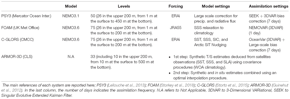
Table 1. Characteristics of the three data assimilation systems (PSY3, FOAM, and C-GLORS) and the statistical merging technique (ARMOR-3D).

The Mercator Ocean International System

The DAS, used to perform OSSEs, is based on the operational monitoring and forecasting system PSY3, which uses the version 3.1 of the NEMO ocean model with a 1/4° ORCA grid type (horizontal resolution of 27 km at the equator, 21 km at mid-latitudes and 6 km poleward). The DAS was initialized on January 09, 2008, using temperature and salinity profiles from the World Ocean Atlas 2013 climatology (Locarnini et al., 2013; Zweng et al., 2013), and was run up until the end of 2010. The ocean model is forced at the surface with the atmospheric fields from the ERA-Interim reanalysis produced by ECMWF (Dee et al., 2011). More details concerning parameterization of the terms included in the momentum, heat and freshwater balances (i.e., advection, diffusion, mixing or surface flux) can be found in Lellouche et al. (2013). Note that, unlike Lellouche et al. (2013), no mean dynamic topography is used for referencing the altimetric sea level anomaly, since the total sea surface height is directly assimilated in the system. In addition to the ocean model, data assimilation procedures based on a reduced-order Kalman filter derived from a SEEK filter (SAM2, Brasseur and Verron, 2006) are used for the assimilation of satellite and in situ observations. A correction for the slowly evolving large-scale error of the model in temperature and salinity is applied. More details on the data assimilation procedures can be found in Lellouche et al. (2013).

The UK Met Office System

The Met Office performed OSSEs using the GO6 configuration of the operational Forecasting Ocean Assimilation Model (FOAM), the model component of which is described by Storkey et al. (2018). The ocean model used here is NEMO at version 3.6 (Madec and The NEMO Team, 2008) in the extended-grid ORCA025 configuration which has a horizontal resolution of approximately 1/4° with 75 levels in the vertical and 1 m vertical resolution near the surface. The ocean model is coupled to the CICE sea-ice model as described in Ridley et al. (2018). The outputs from a multi-decadal free run were used to initialize the OSSEs. In order to produce a simulation which had different characteristics to the NR, the model was forced during the OSSEs by daily fluxes from the Japanese 55-year Reanalysis (JRA55), produced by the Japan Meteorological Agency (JMA, Ebita et al., 2011; Kobayashi et al., 2015) while ERA forcing is usually used. The data assimilation scheme used here is called NEMOVAR (developed collaboratively by CERFACS, ECMWF, INRIA, and the Met Office) and is implemented as a multivariate, incremental 3DVar-FGAT (first-guess-at-appropriate-time) scheme (Waters et al., 2015). No quality control was applied to the simulated observations. OSSEs were run for 2 years from January 2008, with the first 6 months (January–June 2008) as the spin-up period. Both OSSEs and NR outputs were interpolated to a common 1/4° horizontal grid with 50 vertical levels before statistical comparison.

The CMCC System

The OSSEs are run within the framework of the CMCC reanalysis system C-GLORS (Storto et al., 2015). C-GLORS includes the v3.6 of NEMO forced by the ERA-Interim reanalysis and the OceanVar data assimilation system, a 3DVar-FGAT (First Guess at Appropriate Time) scheme (Storto et al., 2011). The experiments are run in a global configuration on the extended ORCA 1/4° grid and 75 vertical levels. The assimilation window is set up to 7 days. The model outputs are provided weekly, from the middle of the assimilation window, to the middle of the assimilation window of the next cycle. Moreover, the possibility of assimilating sea surface temperature maps was switched on. In OceanVar, the background error covariances are modeled through a series of operators. For this study, the OSSEs were performed through an ensemble of six members evolving on their own. To generate the ensemble, three types of perturbations were used: perturbations of the equation of state (Brankart et al., 2015), perturbations of the observations (using the prescribed observation error covariance), and perturbations of the atmosphere forcing fields. In this paper, the mean of the ensemble is given as the CMCC contribution.

The CLS System

The ARMOR3D multivariate analysis system is the Multi Observations component of CMEMS, which relies on the use of statistical methods to combine satellite (sea level anomaly, SLA; sea surface temperature, SST; sea surface salinity, SSS) and in situ temperature and salinity observations (T/S profiles) for an optimal reconstruction of global 3D T/S gridded fields. It is a complementary approach to the DAS presented above. The method, fully described in Guinehut et al. (2012) and recently updated in Verbrugge et al. (2018), starts from the World Ocean Atlas 2013 climatology (Locarnini et al., 2013; Zweng et al., 2013). Satellite data (SLA + SST + SSS) are then projected onto the vertical, using a multiple linear regression method and covariances deduced from historical observations. This step provides synthetic fields from the surface down to 1,500 m depth. These synthetic fields are then combined with T/S in situ profiles using an optimal interpolation method. Analyses are performed at a weekly period on a 1/4° horizontal grid on 24 vertical levels from the surface down to 1,500 m depth. In a final step, the T/S fields are completed from 1,500 to 5,500 m depth (nine additional vertical levels) with the climatology. All parameters such as regression coefficients used in the multiple linear regression method or covariances used in the optimal interpolation method are unchanged compared to the operational ARMOR3D system.

“Design” Experiments

The design experiments used different sets of synthetic observations, which will be introduced in more detail in the following sections. The list of experiments performed by each group is reported in Table 2. For computational resource reasons, the length of the OSSEs period is not identical for all groups, and the present analysis covers a 6-month common period, from January 2009 to June 2009.

TABLE 2

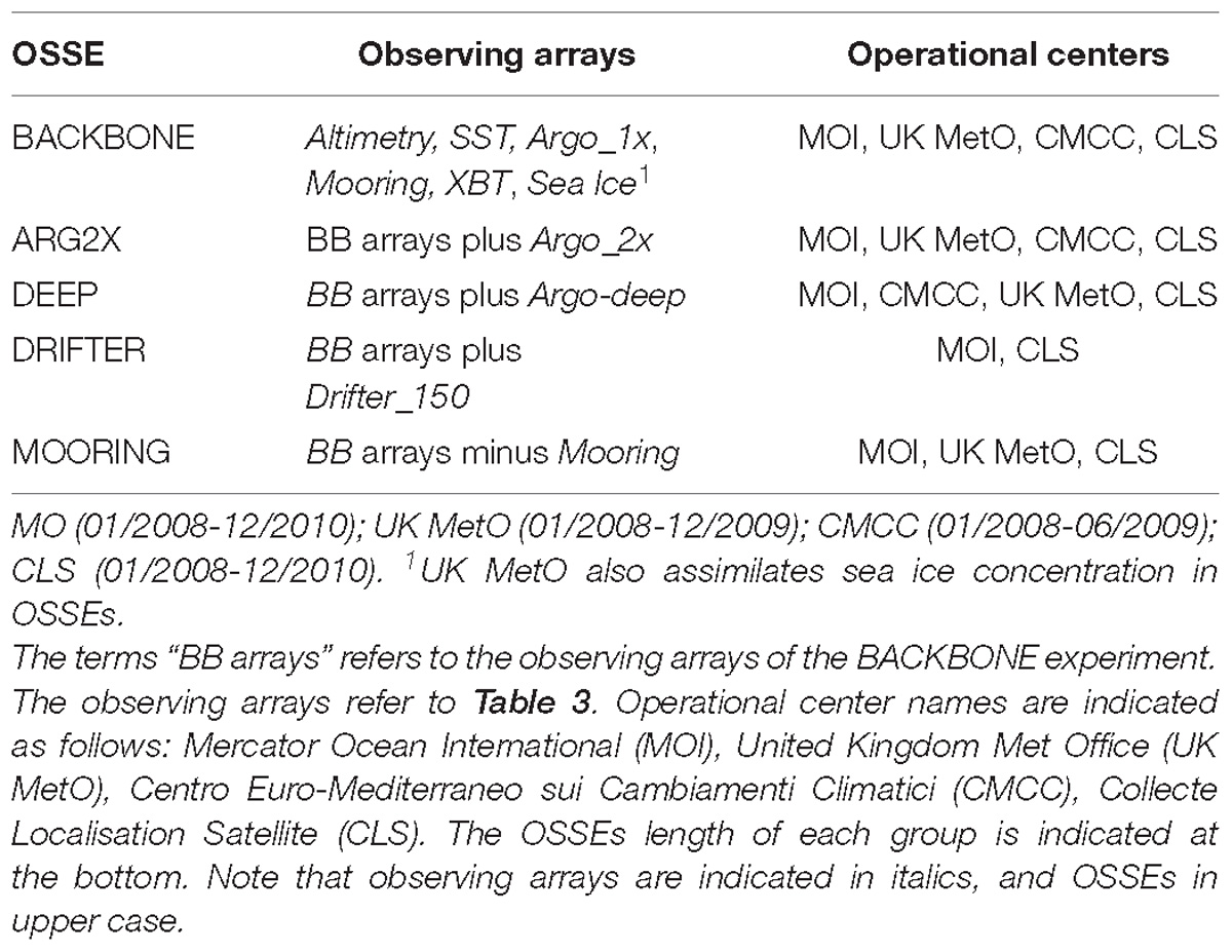
Table 2. List of OSSEs performed by each group.

Construction of the Synthetic Data Sets

The Satellite Component

The generation of the synthetic observations was based on subsampling the daily fields of the NR at the location and date of each observation. In order to deviate from the NR realization, noise was then added to these values – the observation error is discussed later.

The SSH synthetic dataset was built from a constellation of the three satellites Jason-2, Sentinel-3a and Sentinel-3b. The Jason-2 trajectory (longitude, latitude, date) was extracted from CMEMS Sea Level TAC (Thematic Assembly Center) multi-mission along-track L3 altimeter products (as prepared by the DUACS system) for a 3-year period from 2009 to 2011 (10-day repeat cycle; around 13 orbits per day) due to a lack of more than 15 days in the Jason-2 dataset in 2008. The Sentinel-3a/-3b orbits were theoretically determined (27-day repeat cycle: around 14 orbits per day; G. Dibarboure, personal communication). For the ARMOR3D system (CLS), SSH synthetic dataset consist of daily fields on a regular grid at 1/4° horizontal resolution.

For three groups, MOI, CMCC, and CLS, the SST synthetic dataset consisted of daily fields on a regular grid at 1/4° horizontal resolution. The SST and sea ice concentration (SIC) synthetic datasets used for the UK Met Office OSSEs were produced by extracting NR values at the locations of the operational observing networks in 2016. This SST observing network consisted of L2 swat measurements from four infrared satellites (VIIRS onboard Suomi-NPP, and AVHRR onboard MetOp-B and NOAA-18/19), one microwave satellite (AMSR2), and in situ SST measurements (from drifting buoys, moored buoys and ships). The SIC observation locations were from the gridded OSI-SAF product based on retrievals from SSMIS.

The in situ Component

The synthetic in situ datasets consist of subsurface vertical profiles of temperature and salinity from mooring platforms, eXpendable BathyThermograph (XBT, only temperature), and Argo floats, which have been extracted from the CORA 4.1 in situ database distributed by CMEMS In Situ TAC (Cabanes et al., 2013; Szekely et al., 2016). Following discussions with mooring network experts, the mooring sampling during 2015 was chosen to represent the mooring sampling for the 3-year OSSE period (Bourles and Cravatte, personal communication) as one of the most representative periods of the Global Tropical Moored Buoy Array¹. The 2013–2015 drifters sampling was used for the OSSE (Poli, personal communication). The synthetic Argo designs were built considering the time, date and location of Argo profiles during the 2009–2011 period. In order to design a “homogeneous” Argo sampling, approaching one float per 3° × 3° box, float trajectories were removed in the well-sampled Kuroshio region (close to two floats per 3° × 3° box), or were added in the low-sampled Tropical/South Atlantic region. More concretely, trajectories from floats deployed in the Kuroshio region (10°N–45°N; 120°E–150°E) in 2010–2011 were arbitrarily removed. In the Tropical/South Atlantic region (south of 20°N), for a given date, half of the Argo distribution of the day of the following year was added (i.e., the OSSE Argo trajectories of January 01, 2009 are equivalent to the actual Argo trajectories of January 01, 2010, plus half of the floats of the actual Argo trajectories of January 01, 2011 in the tropical/south Atlantic). The advantage of using a homogeneous rather than a non-homogeneous distribution for the observing system designs is that results can more easily be interpreted, in the sense that they are less regionally and temporally dependent.

In Figure 1 (bottom panel), the time-averaged number of Argo floats, expressed as equivalent number per 3° × 3° box, is shown for the actual period of 2014–2015 and in the synthetic backbone configuration (assimilating synthetic data from observation types that exist in the current observing network). The zonally averaged number of floats for each basin demonstrates the more “homogeneous” feature of the synthetic design compared to the actual one in 2014–2015. The in situ component of the Backbone design is composed of moorings, XBT, and Argo floats (Table 2).

FIGURE 1

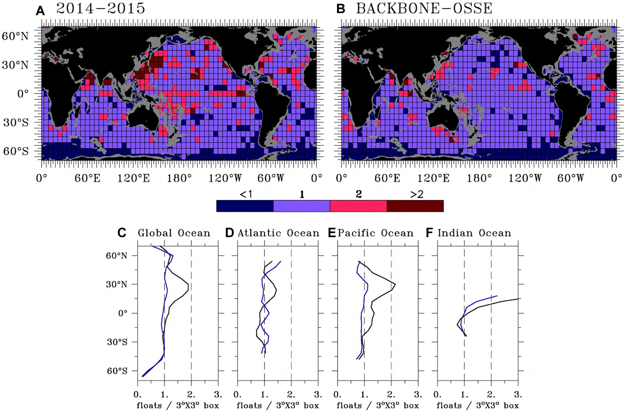
Figure 1. Time-averaged number of floats per 6°× 6° box (A) from the CORA4.1 dataset for the period 2014–2015, and (B) from the synthetic BACKBONE Argo design for the period 2009–2010. Unit is equivalent float number per 3° × 3° box. In (C–F), the zonally averaged number of floats is indicated for each basin, with (C) the global Ocean, (D) the Atlantic Ocean, (E) the Pacific Ocean, and (F) the Indian Ocean. The black and blue lines indicate the 2014–2015 CORA4.1 and the 2009–2010 synthetic BACKBONE quantities, respectively.

One of the extensions of the Argo array consists of doubling the number of Argo floats in the western boundary currents (WBC) and in the equatorial regions (3°S–3°N, source JCOMMOPS), i.e., two floats per 3° × 3° box. For these regions, we added profiles of year N+1, except in regions of the Tropical/south Atlantic where profiles of years N+1 and N+2 were added (Figure 2A). A second extension consisted of implementing a monthly 5° × 5° deep Argo array, i.e., one float per 5° × 5° box (∼1200 floats, Johnson et al., 2015) (Figures 2B,C). 1/3 of the Argo floats from the backbone were monthly (every three profiles) extended to the bottom (5,500 m). Below 2,000 m, these “deep-Argo” floats were extracted at the NR model depths.

FIGURE 2

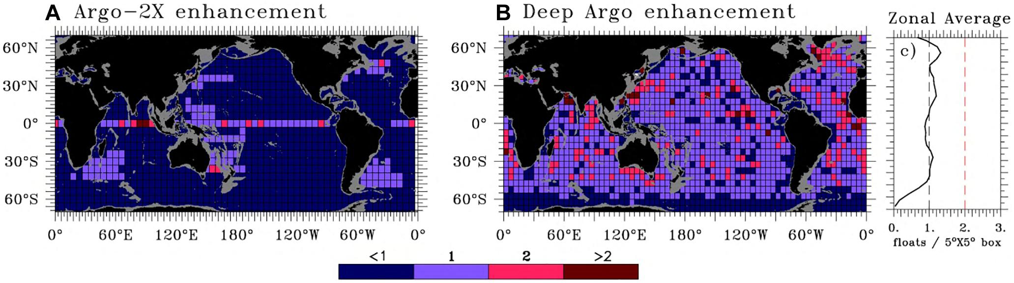
Figure 2. Synthetic Argo enhancements for the (A) Argo-2x and (B) Argo-deep designs additionally to the Backbone Argo design (Argo-1x). The number of floats is calculated for the upper-ocean (0–2000 m) in Argo-2x per 6° × 6° box, and for the deeper ocean (below 2000 m) in Argo-deep per 5° × 5° box. In (C), the zonally averaged number of floats of the Argo-deep design is indicated for the global Ocean. Note that unit in (A) is equivalent float number per 3°× 3° box.

Introduction of Realistic Errors

The reliability of an OSSE system to correctly provide observation impact assessment partly lies in defining appropriate errors, which were included in the synthetic observations. This includes two types of errors: (i) a representation error, which is vertically and horizontally correlated and mostly related to variability due to unresolved or poorly resolved processes of the analysis and forecast system or the statistical merging technique (e.g., inertial waves); and (ii) a random instrumental error, which is due to the uncertainty of measurement. In practice, these additional errors have been obtained as follows. First, for each observation position (longitude, latitude, and date), the NR fields is randomly shifted by ±3 days (following a uniform distribution, either 3 days before or 3 days after the given date). This time-shifting technique, largely used for the atmosphere (e.g., Huang and Wang, 2018), allows for the consideration of correlated errors resulting from small-scale processes at a weekly scale, and thus account for the representativeness error. Then, the synthetic observations are extracted from the time-shifted NR fields, which are at a higher horizontal resolution (at 1/12° resolution) than the data assimilation systems (at 1/4° resolution). In addition to the weekly variability included by the time-shifting technique, the higher resolution of the NR also includes small-scale variability embedded in eddy-resolving systems, but not in eddy-permitting systems. Finally, uncorrelated instrumental errors are added to each observation depending on the observation type, following a Gaussian distribution with the standard deviation given by the instrumental uncertainty (Table 3).

TABLE 3

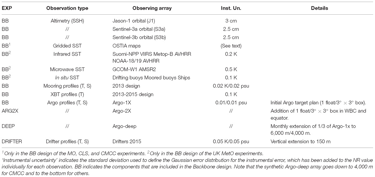
Table 3. Observation types and observation systems, which have been used for subsampling the NR at the space and time location of each observation and assimilated in the OSSEs.

Figure 3 shows the error variance on the synthetic observations per 4° × 4° box, calculated for the 3-year period. In order to illustrate the spatial variability, this is shown for the 100-m temperature and 10-m salinity only, based on pairs of differences between the synthetic observations of the Argo-1x observing array (Table 3) and its equivalent Nature Run values. The two maps show that the error is higher in areas of high variability (i.e., in the western boundary current and along the tropical thermocline for both the 100-m temperature and 10-m salinity), as confirmed in the zonal averages (Figures 3B,D). To assess the impact of only considering errors due to a higher resolution NR compared with the DAS (i.e., no time-shifting, no instrumental error), the zonal average error variance is shown, based on pairs of differences between synthetic observations extracted from the 1/12° fields, with and without spatial smoothing to fit the 1/4° grid (Figure 3). Given the amplitude of the instrumental error of the order of O (0.01°C) for temperature and O (0.01 psu) for salinity for Argo measurement, it clearly appears that the time-shifting procedure dominates the added error, both in temperature and salinity. Note that large instrumental error, such as for XBT, implies a stronger contribution to the total error than other observation types.

FIGURE 3

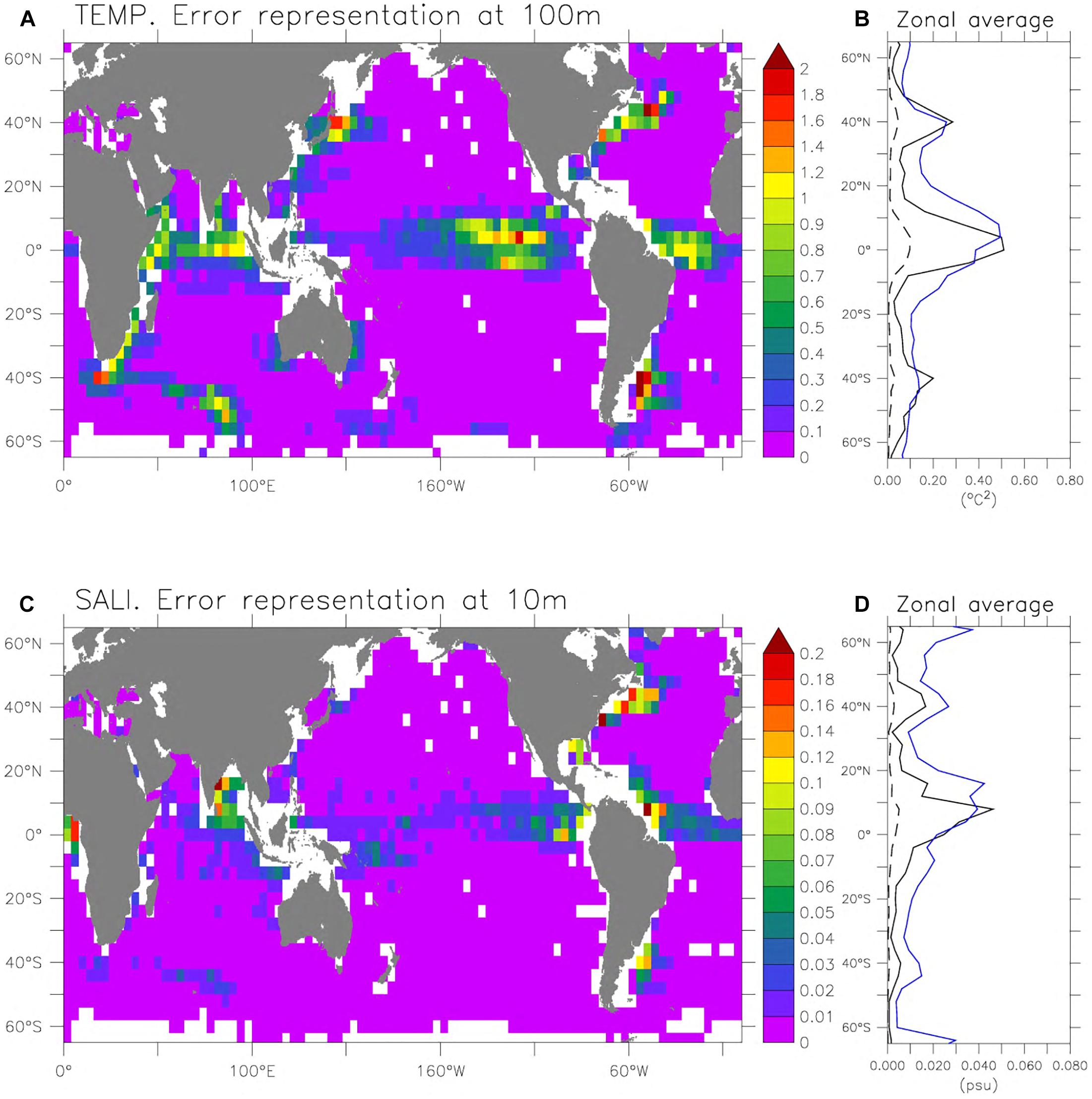
Figure 3. Total error variance on synthetic observations per 4° × 4° box for (A,B) the 100-m temperature and (C,D) the 10-m salinity, based on differences between the synthetic observations of the Argo-1x design and its equivalent Nature Run values. In (B,D), the zonal averages of (A) and (C) (full black lines) are compared with the error variance based on pairs of differences between synthetic observations extracted from the 1/12 fields, with and without spatial smoothing to fit the 1/4 grid (dashed black lines), and from the operational representation error used in the 1/4° MOI system (blue lines, Lellouche et al., 2013).

Figures 3B,D, also shows, for illustrative purpose, the zonally averaged representation error considered in the operational MOI system at 1/4° horizontal resolution for the 100-m temperature and 10-m salinity (blue lines). This error is deduced from a long numerical experiment (free run without assimilation) with respect to a running mean and represents an estimate of the 7-day scale error (Lellouche et al., 2013). For the 100-m temperature and 10-m salinity, the operational representation error shows a similar latitude dependence to that of the synthetic observation error and results from a complex mixture of unresolved or poorly resolved processes due to physics approximations (e.g., inertial waves), numerical issues (e.g., grid resolution), or atmospheric forcing uncertainty. In addition, the representation error is strongly dependent on the representation of the ocean variability by numerical models, affecting model parameterization and assimilation procedures. The accuracy of this prescribed error will continue to improve with a better knowledge of the ocean variability, such as in the deep ocean.

Results

In order to demonstrate that the errors in the OSSEs were consistent with those of the operational systems, the temperature and salinity root mean square error (RMSE), with respect to the NR, were calculated with the BACKBONE experiment for the four systems. The assessment metrics of the present work were based on area averages for the Atlantic Ocean (South of 70°N, and north of line Ushuaia-Cape Town) and in the Gulf Stream region (80°W–30°W; 36°N–51°N). In Figure 4, the RMSE pattern is similar between the four systems, both in temperature and salinity for the Atlantic Ocean. The temperature RMSE was largest at 100 m, with an amplitude of around 1°C (1.2°C for the CMCC, and 0.8°C for the others) and decreases to 0.1°C at 1,500 m and below. The salinity RMSE was largest at the surface (>0.3 psu) and decreased in the deeper ocean to around 0.02 psu. This vertical dependency of the errors mostly reflects the global oceanic variability dominated by the tropical fluctuations (Roemmich and Gilson, 2011). In the following section, the ability of a given ocean observing system, OSi, designed to represent the ocean state, is assessed by quantifying the Mean Square Error (MSE) reduction of the OSi from the BACKBONE observing system design, i.e., MSE_{OSi_red.} = (MSE_BACKBONE - MSE_OSi)/MSE_BACKBONE, calculated in the model space on a 6-month common period, from January 2009 to June 2009. These four simulations constitute an ensemble, which will be characterized by its mean and standard deviation.

FIGURE 4

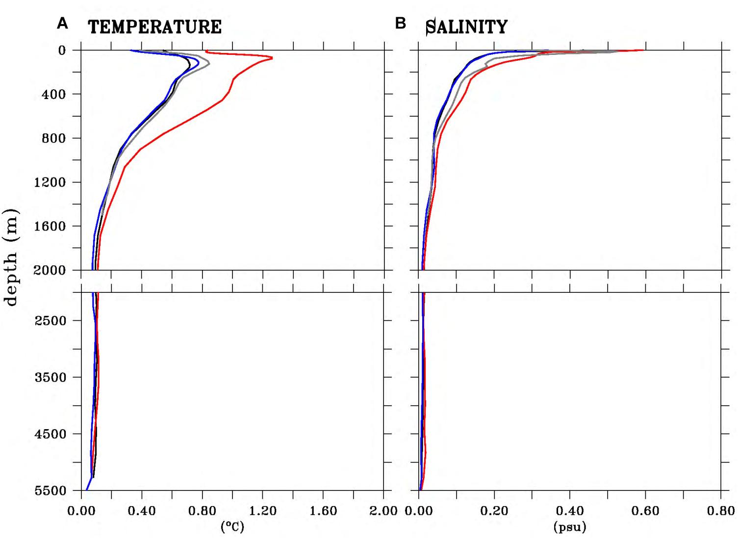
Figure 4. Temperature (A) and salinity (B) RMSE with respect to the NR for the period January 2009 to June 2009, area-averaged in the Atlantic Ocean, from MOI (black), the Met-Office (blue), the CLS (gray), and the CMCC (red) systems.

It should be noted that, in addition to experiments dedicated to global Lagrangian arrays, such as the Argo or Drifter programs, three groups (Mercator Ocean International, UK Met Office and CLS) have performed a dedicated experiment focusing on the contribution of the current global tropical mooring arrays, by withholding fixed-point mooring from the BACKBONE design. Consistently with Xue et al. (2017), the impact of moorings was localized around mooring sites (not shown). Several studies have investigated the role of tropical moorings in ocean monitoring systems and reanalysis, especially in the tropical Pacific (e.g., Fujii et al., 2015; Xue et al., 2017). Even if most state that the quality of the analyses was improved due to the assimilation of moorings, the quantification of the relative contribution of each component of the observing system (e.g., fixed-points versus Lagrangian floats) remains an important challenge for operational centers. It should be mentioned that the high temporal frequency/sampling of moorings is not exploited by construction in current 3D data assimilation systems. With 4D ones, the impact could be potentially larger, as several profiles from moorings could be assimilated. In this study, the metrics used focus on the entire Atlantic and Gulf Stream regions, which might not be appropriate for a regional fixed-point array. Thus, this experiment is not presented in this study and further investigations and appropriately adapted metrics are therefore needed in order to assess the contribution of tropical moorings to the representation of the ocean state in the current forecasting and analysis systems.

Doubling Argo in the WBC and Along the Equator

Characterized by strong air-sea interactions, the WBC and equatorial regions have been identified as key elements of climate variability contributing to global budgets of heat, moisture, and carbon. However, the representation of the ocean state in these two types of regions remains relatively complex, due to the presence of strong currents, intense frontal structures, and a strong atmospheric synoptic variability (Cronin et al., 2012). Consequently, it has been recommended by the Argo program to improve the Argo float coverage in these dynamical regions (Roemmich and Gilson, 2009).

In Figure 5, the ensemble mean MSE reduction of temperature and salinity from the four DAS in the upper 2,000 m, area-averaged in the Atlantic Ocean and the Gulf Stream regions, indicates that enhancing the Argo coverage in WBC and equatorial regions would provide a better representation of the temperature and salinity variability in operational models. On average, doubling Argo in the WBC and along the equator would improve the temperature and salinity representation of around 5–10% for the entire Atlantic. The small standard deviation indicates statistical significance of the results and demonstrates that the four systems are consistent. Focusing on the enhanced regions, such as the Gulf Stream region, shows a higher improvement (up to 20%) for the four groups. However, the shape of the error reduction profile can differ between the members of the ensemble. While the maximum improvement is found around 1,000 m for the Met Office, MO, and CLS DAS, the maximum is around 300 m for CMCC (not shown). This is illustrated by the larger standard deviation in the Gulf Stream region compared to the entire Atlantic Ocean, stating that differences between the four members can be important (e.g., for salinity).

FIGURE 5

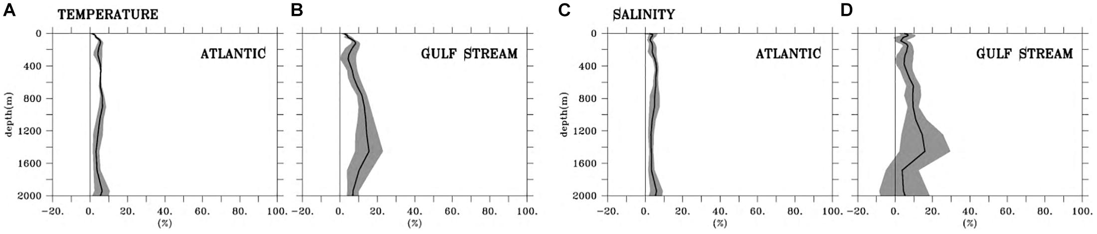
Figure 5. 0–2,000 m temperature and salinity profiles of MSE reduction as compared with the BACKBONE experiment for the ARG2X experiment, area-averaged in (A,C) the Atlantic Ocean and (B,D) the Gulf Stream. The black line is the ensemble mean. Gray indicates the standard deviation of the four members. The unit is in percentage of the MSE from the BACKBONE experiment.

Thus, the four systems agreed, showing a significant decrease of the RMSE, when the Argo coverage was enhanced in WBC and equatorial regions. As expected, the impact was stronger in these specific regions where the sampling was doubled, but the associated standard deviation of the ensemble was also higher. Further investigations will be developed in future studies based on quantitative metrics focusing on processes of interest in the specific regions, or on the ability of resolving specific space and time scales (e.g., impact on eddy detection). It should be noted that the ensemble spread can also be affected by systematic errors embedded in the assimilation models.

Implementing a Deep Argo Array

Due to its contribution to rising sea levels and the Earth’s energy budget, the deep ocean is a crucial component of the ocean variability (Purkey and Johnson, 2010). However, the performance of numerical models are limited by the lack of sufficient deep ocean observations. Such data are required for model initialization and assimilation, and are presently limited to sparsely repeated hydrographic sections embedded in international programs (e.g., WOCE and GO-SHIP). The need for intense observations in the deep ocean, below 2,000 m, has been recognized by the scientific community. A deep Argo array is therefore expected to be deployed to carry out deep ocean sampling at a global scale (Johnson et al., 2015), with the aim to achieve similar success than the core-Argo array, which has been sampling the upper-ocean (0–2,000 m) for more than 15 years (Riser et al., 2016).

In order to illustrate how the implementation of a deep Argo array would impact ocean analyses, Figure 6 shows the temperature and salinity MSE reduction from the surface to the bottom of the Atlantic Ocean and Gulf Stream regions. Compared to the BACKBONE design (no deep observations), a deep Argo array significantly improves the temperature and salinity from 1,500 m to the bottom. With respect to the spread, the improvement on salinity is significant below 2,000 m of depth, while on temperature, although large on average, only at selected depth levels. The four members showed some improvements below 2,000 m, although one member (CMCC) had a weaker impact (less than 10%) than that of the other three members (not shown). In general, the ensemble mean demonstrates an improvement of 20% for temperature and salinity below 2,000 m but can reach 50% for salinity for the Gulf Stream region. As for the Argo doubling experiment, the associated standard deviation of the ensemble ranged between 20 and 30%. This demonstrates that, even if the four members show general improvement in the deep ocean, they might differ quantitatively. Another point is that the assimilation of additional deep observations induces a degradation of the systems at shallower depths (between 400 and 1,000 m). This highlights the need for further investigations of the observation error and its impact on the observing network.

FIGURE 6

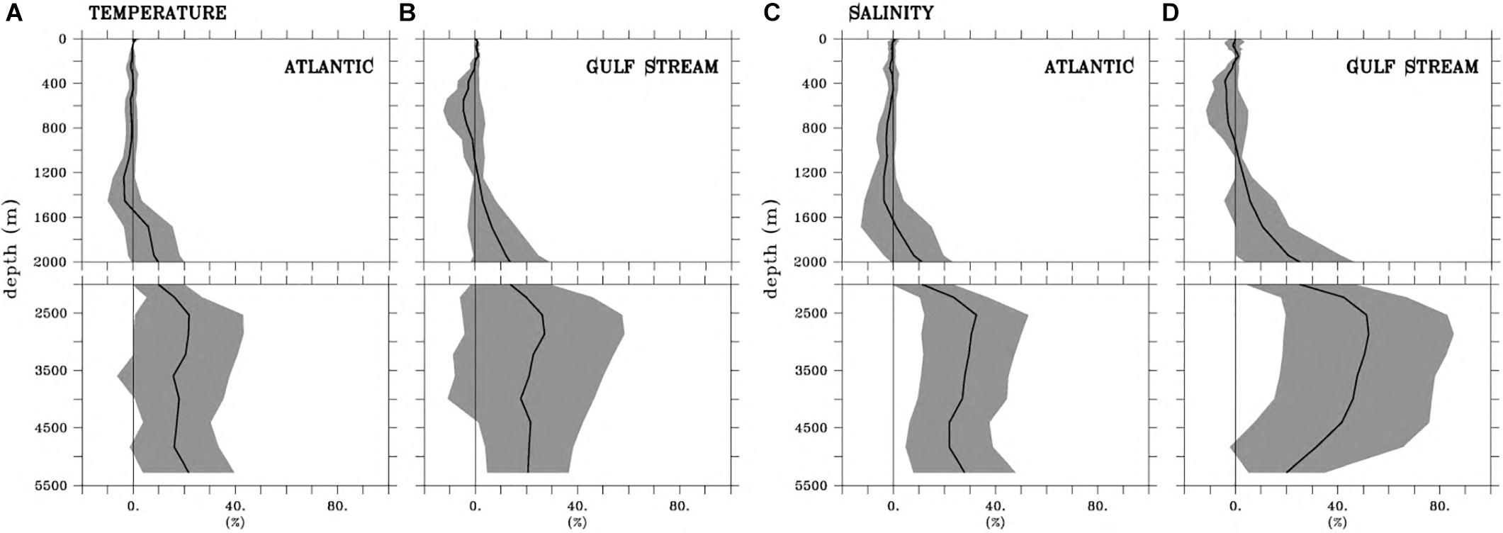
Figure 6. Same as Figure 5, but for the top-to-bottom profiles of MSE reduction for the DEEP experiment as compared with the BACKBONE experiment.

Although, as mentioned previously, these results might depend on differences in model representation parameterization, these experiments suggest that the deep Argo observations would be complementary to the upper ocean observing system, mostly by controlling the deep-water mass properties. Even if the added value of deep observations appears clearly in temperature and salinity, other diagnostics are necessary to evaluate the gain of deep Argo arrays on integrated quantities (e.g., heat and freshwater contents, transports) and on deep ocean processes, and multi-annual experimental periods are most likely required to maximize the impact of such observations.

Extending the Depth of the Drifter Array

In addition to surface velocity derived from trajectories, the global drifter array plays an essential role in providing in situ sea surface temperature measurements (Lumpkin et al., 2017), which are critical for calibrating and reducing biases in satellite-derived temperatures (e.g., Emery et al., 2001) and thus for depicting long term variations in the earth’s surface temperature. At the ocean-atmosphere interface, the sea surface temperature can directly affect atmospheric forecasts and analysis (Maloney and Chelton, 2006). By equipping the current drifter array with a thermistor chain instrumented from the surface to 150 m (with both temperature and salinity), the objective of the DRIFTER experiment, seen as an idealized case study, is to provide an upper limit to the benefit of extending all or part of the current drifter array.

Unlike previous experiments, only two groups (MOI and CLS) have performed the DRIFTER experiment. Following the same diagnostics, the implementation of a drifter array equipped with a thermistor chain would improve the temperature and salinity representation by 5% to 15% for the entire Atlantic and the Gulf Stream region, respectively (Figure 7).

FIGURE 7

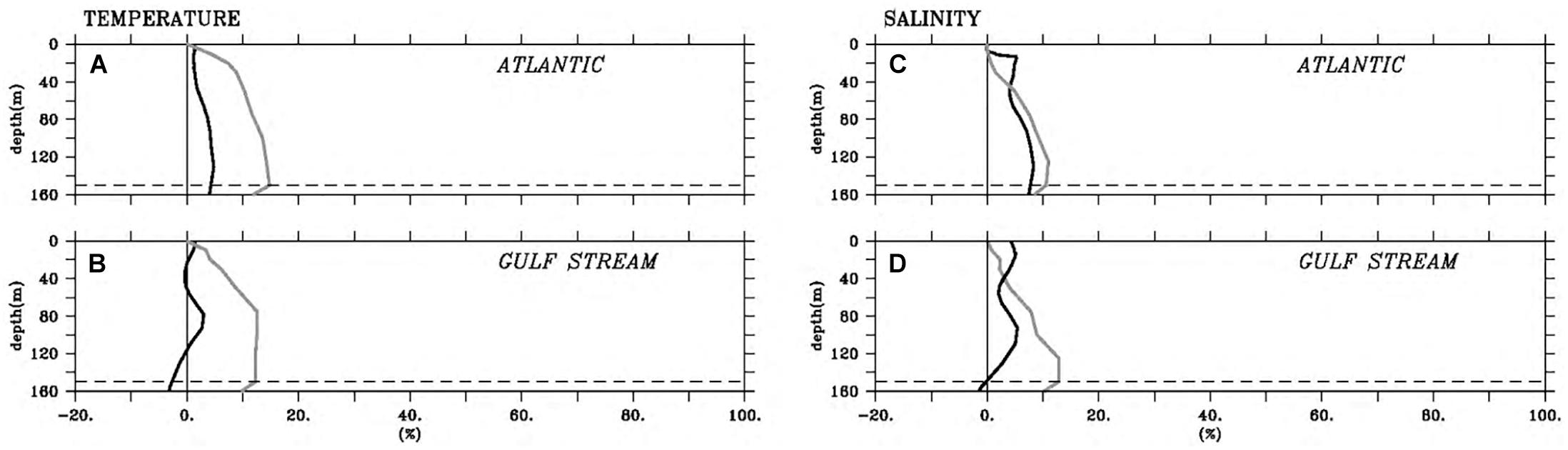
Figure 7. Same as Figure 5, but for the DRIFTER experiment as compared with the BACKBONE experiment from MOI (black), and the CLS (gray) systems in the upper 160 m. The horizontal dashed line indicates the maximum depth of the synthetic drifter observations.

Based on the area-averaged error reduction, the implementation of a drifter array equipped with a thermistor chain would benefit the ocean state representation, mostly in subsurface. The amplitude of the improvement reaches up to 10–15% for both the entire Atlantic and the Gulf Stream region. The enhanced sampling of the 0–150 m layer clearly allows a better constrain of the mixed layer characteristics that is driven by ocean atmosphere exchanges. Further investigation are required to identify which process representation is affected by this enhanced sampling in the surface layer.

Summary and Conclusion

Based on numerical experiments, further evolutions of the in situ component of the GOOS have been assessed by using four global eddy-permitting systems, including three analyses and forecasting systems and one statistical analysis system. The originality of this study lies in the assimilation of exactly the same synthetic in situ data sets, which are deduced by sub-sampling the Nature Run (1/12° unconstrained system at Mercator Ocean International) in space and time for each observation of a given observing system design, and the use of this ensemble of simulations to get a ‘confidence interval’ on the impact of these evolutions. For each observing system evolution, at least two groups assessed the impacts of the integrated observing system on the monitoring and forecasting systems and have generally shown improvements in the representation of temperature and salinity fields.

Compared to the Nature Run, the doubling of Argo in the WBCs and along the equator demonstrated an improvement of both temperature and salinity for the entire Atlantic Ocean between 5 and 10% compared to the BACKBONE design. Stronger improvements were found in the WBCs and, less evidently, along the equator, in which Argo was doubled (not shown). These results are consistent with Oke et al. (2015) and Turpin et al. (2015), who have investigated the impacts of removing half of the existing Argo floats in real time ocean forecasting systems. However, further investigation could study how the impact could be improved by focusing on the Kuroshio region, where current sampling is already around 2 floats per 3° × 3° box.

The implementation of a deep Argo array (1 float every 5° × 5° square), which reports monthly measurements of the water column down to 4,000 m or to the bottom, shows a significant impact in controlling the temperature and salinity biases in the deep ocean basins. Three systems have shown significant improvement of the temperature and salinity representation with 20–40% of error reduction. The fourth system showed an improvement of up to 20% in a limited area. These encouraging results should be confirmed by performing experiments on a longer period (around a decade) to assess the reduction in error of the long-term trends in the deep ocean due to the deep Argo array. It is noteworthy that the deep Argo horizontal sampling is based on a sub-set of the core-Argo sampling, and consequently, the deep Argo sampling is lower than the target in the Southern Ocean. This questions the simulation of the synthetic observations, i.e., using current or simulated Argo trajectories. Some work, using Observing System Experiments, is needed for investigating how the current deep Argo pilot arrays would impact the monitoring systems.

The extension of the drifter array to 150 m, which today remains an optimistic perspective, has to be seen as an idealized case study. The improvement of the temperature and salinity representation is significant in the surface layer (10–20% of error reduction), and the major areas with the strongest impact are yet to be identified. The impact of the current mooring array on the monitoring and forecasting systems is localized near the moorings and does not significantly affect the large-scale structures, as mentioned by Fujii et al. (2015). Several points can explain this. The decorrelation scales might not be adapted to these high-resolution fixed-point data, and the current assimilation schemes might not be sufficiently progressed to extract the maximum information from moorings.

Overall, this original study has demonstrated a positive impact of the different simulated extra observation networks. These impacts are quite consistent despite the use of different analysis systems, although the CMCC system provides weaker positive impacts for the deep Argo OSSE (probably due to differences in prescribed representation error). However, the interest of this work resides also in identifying the limitations of the method in order to overcome these issues in future OSSEs. As mentioned previously, the results are model-dependent (e.g., due to systematic errors), and the multi-system approach has been identified as a potential way to overcome this limitation. It was also assumed that impacts of the observing system components evolved following the development of monitoring and forecasting systems, including time and space resolution. Improvements in the assimilation schemes (e.g., from 3D-VAR to 4D-VAR) have also been identified as contributing to changes in impacts of an observation (Usui et al., 2015), e.g., high sampling of data (moorings, radars, day-time satellite measurements) could be better exploited with 4D-VAR.

Although the three DAS use the NEMO ocean model or similar atmospheric forcing, there are remarkable differences in the systems (e.g., initialization, bulk formulas, and surface restoring) for which the ensemble spread tends to be reliable. It is, however, important to recognize that the higher the multi-system ensemble, using different systems and methods, the more robust the results are likely to be. Multi-model, multi-forcing ensembles could thus be envisaged in the future. Moreover, the experiments relied on the performance of the Nature Run, and any improvement of the free simulation, especially below the surface layer, should improve the results. The systems are tuned for a specific observation network and require time to adapt to a new one (e.g., representation error in the deep ocean). A longer period of OSSE is thus required to obtain more significant and robust statistics, especially in the deeper ocean. All these aspects could be addressed in a future study.

In conclusion, a coordinated effort from the European forecasting centers carried out within the H2020 AtlantOS project has provided consistent information about observation impact on monitoring and forecasting systems concerning the evolution of the in situ component of the GOOS. In the continuity of the GODAE Ocean View activities, this work tackles the assessment of observation impact in monitoring and forecasting systems and can be seen as a step further toward the guidance of a sampling strategy in the preparation of the Oceanobs’19 conference. However, the present work is a first step toward future coordinated impact studies, in which the development of assimilation schemes and progress in numerical models should significantly improve the robustness of results, together with the routine use of ensemble statistics and should enable the use of more sophisticated process-based assessment metrics.

Data Availability

All datasets generated for this study are included in the manuscript and/or the supplementary files.

Author Contributions

FG decided the structure of the manuscript and coordinated the writing team. FG contributed to introduction, OSSE principle, the nature run configuration, and the Mercator Ocean International system sections. CM, RR, RK, and MM contributed to the UK Met Office system section. IM, AS, and SM contributed to the CMCC system section. SG contributed to the CLS system section. FG, ER, MH, RK, MM, IM, RR, and PLT contributed to “Design” experiments section. FG, SG, IM, CM, ER, RK, and MH contributed to results and summary and conclusion sections. The manuscript is edited by FG with the support of SG, CM, IM, ER, RK, RR, AS, MM, SM, and PLT.

Funding

This project received funding from the European Union’s Horizon 2020 Research and Innovation Program under grant agreement no. 633211 (AtlantOS).

Conflict of Interest Statement

SG was employed by company Collecte Localisation Satellites.

The remaining authors declare that the research was conducted in the absence of any commercial or financial relationships that could be construed as a potential conflict of interest.

Acknowledgments

This study was conducted using Copernicus Marine Service Products. This paper used data collected and made freely available by programs that constitute the Global Ocean Observing System and the national programs that contribute to it (http://www.ioc-goos.org/), i.e., the Argo data collected and made freely available by the International Argo Project and the national programs that contribute to it (http://argo.jcommops.org), the surface drifter data supplied by the Global Drifter Program, the TAO-PIRATA-RAMA (PMEL-NOAA) and the OceanSITES initiative for various data sets. We thank two reviewers for their helpful comments.

Footnotes

1. ^ www.pmel.noaa.gov/gtmba

References

Atlas, R. (1997). Atmospheric observations and experiments to assess their usefulness in data assimilation. J. Meteorol. Soc. Jpn. 75, 111–130. doi: 10.2151/jmsj1965.75.1B_111

CrossRef Full Text | Google Scholar

Atlas, R., Kalnay, E., Baker, W. E., Susskind, J., Reuter, D. C., and Halem, M. (1985). “Simulation studies of the impact of future observing systems on weather prediction,” in Proceedings of the 7th Conference on Numerical Weather Prediction, Montreal, QC, 145–151.

Google Scholar

Ballabrera-Poy, J., Hackert, E., Murtugudde, R., and Busalacchi, A. J. (2007). An observing system simulation experiment for an optimal moored instrument array in the tropical Indian Ocean. J. Clim. 20, 3249–3268. doi: 10.1175/JCLI4149.1

CrossRef Full Text | Google Scholar

Balmaseda, M. A., Hernandez, F., Storto, A., Palmer, M. D., Alves, O., Shi, L., et al. (2015). The ocean reanalyses intercomparison project (ORA-IP). J. Operat. Oceanogr. 8(Suppl. 1), s80–s97. doi: 10.1080/1755876X.2015.1022329

CrossRef Full Text | Google Scholar

Bell, M. J., Schiller, A., Le Traon, P. Y., Smith, N. R., Dombrowsky, E., and Wilmer- Becker, K. (2015). An Introduction to GODAE OceanView. Abingdon: Taylor & Francis.

Google Scholar

Bonaduce, A., Benkiran, M., Remy, E., Le Traon, P. Y., and Garric, G. (2018). Contribution of future wide swath altimetry missions to ocean analysis and forecasting. Ocean Sci. 14, 1405–1421. doi: 10.5194/os-2018-58

CrossRef Full Text | Google Scholar

Brankart, J. M., Candille, G., Garnier, F., Calone, C., Melet, A., Bouttier, P. A., et al. (2015). A generic approach to explicit simulation of uncertainty in the NEMO ocean model. Geosci. Model Dev. 8, 1285–1297. doi: 10.5194/gmd-8-1285-2015

CrossRef Full Text | Google Scholar

Brasseur, P., and Verron, J. (2006). The SEEK filter method for data assimilation in oceanography: a synthesis. Ocean Dyn. 56, 650–661. doi: 10.1007/s10236-006-0080-3

CrossRef Full Text | Google Scholar

Cabanes, C., Grouazel, A., von Schuckmann, K., Hamon, M., Turpin, V., Coatanoan, C., et al. (2013). The CORA dataset: validation and diagnostics of in-situ ocean temperature and salinity measurements. Ocean Sci. 9, 1–18. doi: 10.5194/os-9-1-2013

CrossRef Full Text | Google Scholar

Cravatte, S., Kessler, W. S., Smith, N., Wijffels, S. E., and Contributing Authors (2016). First Report of TPOS 2020. GOOS-215, 200. Available at: http://tpos2020.org/first-report/

Google Scholar

Cronin, M. F., Nicholas, B., Talley, L. D., Booth, J., Joyce, T. M., Ichikawa, H., et al. (2012). “Monitoring ocean–atmosphere interactions in western boundary current extensions,” in Proceedings of OceanObs’09: Sustained Ocean Observations and Information for Society, Venice.

Google Scholar

Dee, D. P., Uppala, S. M., Simmons, A. J., Berrisford, P., Poli, P., Kobayashi, S., et al. (2011). The ERAInterim reanalysis: configuration and performance of the data assimilation system. Q. J. R. Meteorol. Soc. 137, 553–597. doi: 10.1002/qj.828

CrossRef Full Text | Google Scholar

Ebita, A., Kobayashi, S., Ota, Y., Moriya, M., Kumabe, R., Onogi, K., et al. (2011). The Japanese 55-year Reanalysis ”JRA-55”: an interim report. SOLA 7, 149–152. doi: 10.1016/j.scitotenv.2018.10.126

PubMed Abstract | CrossRef Full Text | Google Scholar

Emery, W. J., Baldwin, D. J., Schlussel, P., and Reynolds, R. W. (2001). Accuracy of in situ sea surface temperatures used to calibrate infrared satellite measurements. J. Geophys. Res. 106, 2387–2405. doi: 10.1029/2000JC000246

CrossRef Full Text | Google Scholar

Fujii, Y., Cummings, J., Xue, Y., Schiller, A., Lee, T., Balmaseda, M. A., et al. (2015). Evaluation of the tropical Pacific observing system from the ocean data assimilation perspective. Q. J. R. Meteorol. Soc. 141, 2481–2496. doi: 10.1002/qj.2579

CrossRef Full Text | Google Scholar

Gasparin, F., Garric, G., Remy, E., Drillet, Y., Drevillon, M., Greiner, E., et al. (2018). A large-scale view of oceanic variability from 2007 to 2015 in the global high-resolution monitoring and forecasting system at Océan. J. Mar. Syst. 187, 260–276. doi: 10.1016/j.jmarsys.2018.06.015

CrossRef Full Text | Google Scholar

Good, S. A., Martin, M. J., and Rayner, N. A. (2013). EN4: quality controlled ocean temperature and salinity profiles and monthly objective analyses with uncertainty estimates. J. Geophys. Res. 118, 6704–6716. doi: 10.1002/2013JC009067

CrossRef Full Text | Google Scholar

Guinehut, S., Dhomps, A., Larnicol, G., and Le Traon, P.-Y. (2012). High resolution 3-D temperature and salinity fields derived from in situ and satellite observations. Ocean Sci. 68, 845–857. doi: 10.5194/os-8-845-2012

CrossRef Full Text | Google Scholar

Halliwell, G. R., Srinivasan, A., Kourafalou, V., Yang, H., Willey, D., Le Hénaff, M., et al. (2014). Rigorous evaluation of a fraternal twin ocean OSSE system for the open Gulf of Mexico. J. Atmos. Ocean. Technol. 31, 105–130. doi: 10.1175/JTECH-D-13-00011.1

CrossRef Full Text | Google Scholar

Huang, B., and Wang, X. (2018). On the use of cost-effective valid-time-shifting (VTS) method to increase ensemble size in the GFS Hybrid 4DEnVar system. Mon. Weather Rev. 146, 2973–2998. doi: 10.1175/MWR-D-18-0009.1

CrossRef Full Text | Google Scholar

Johnson, G. C., Lyman, J. M., and Purkey, S. C. (2015). Informing deep Argo array design using Argo and full-depth hydro- graphic section data. J. Atmos. Ocean. Technol. 32, 2187–2198. doi: 10.1175/JTECH-D-15-0139.1

CrossRef Full Text | Google Scholar

Kobayashi, S., Ota, Y., Harada, Y., Ebita, A., Moriya, M., Onoda, H., et al. (2015). The JRA-55 reanalysis: general specifications and basic characteristics. J. Meteorol. Soc. Jpn. 93, 5–48. doi: 10.2151/jmsj.2015-001

CrossRef Full Text | Google Scholar

Kuo, T. H., Zou, X., and Huang, W. (1998). The impact of global positioning system data on the prediction of an extratropical cyclone: an observing system simulation experiment. Dyn. Atmos. Oceans 27, 439–470. doi: 10.1016/S0377-0265(97)00023-7

CrossRef Full Text | Google Scholar

Lea, D. J., Martin, M. J., and Oke, P. R. (2014). Demonstrating the complementarity of observations in an operational ocean forecasting system. Q. J. R. Meteorol. Soc. 140, 2037–2049. doi: 10.1002/qj.2281

CrossRef Full Text | Google Scholar

Lellouche, J. M., Greiner, E., Le Galloudec, O., Garric, G., and Regnier, C. (2018). Re- cent updates on the Copernicus marine service global ocean monitoring and forecasting real-time 1/12 high-resolution system. Ocean Sci. Discuss. 2018, 1–70. doi: 10.5194/os-2018-15

CrossRef Full Text | Google Scholar

Lellouche, J. M., Le Galloudec, O., Drevillon, M., Régnier, C., Greiner, E., Garric, G., et al. (2013). Evaluation of global monitoring and forecasting systems at Mercator Océan. Ocean Sci. 9:57. doi: 10.5194/os-9-57-2013

CrossRef Full Text | Google Scholar

Li, Z., Chao, Y., McWilliams, J. C., and Ide, K. (2008). A three-dimensional variational data assimilation scheme for the regional ocean modeling system: implementation and basic experiments. J. Geophys. Res 113:C0500. doi: 10.1029/2008JC004928

CrossRef Full Text | Google Scholar

Locarnini, R. A., Mishonov, A. V., Antonov, J. I., Boyer, T. P., Garcia, H. E., Baranova, O. K., et al. (2013). NOAA Atlas NESDIS 73 World Ocean Atlas 2013 Volume 1: Temperature, ed. S. Levitus (Silver Spring, MD: NOAA Printing Officce), 40.

Google Scholar

Lumpkin, R., Centurioni, L., and Perez, R. (2016). Fulfilling observing system implementation requirements with the global drifter array. J. Atmos. Ocean. Technol. 33, 685–695. doi: 10.1175/JTECH-D-15-0255.1

CrossRef Full Text | Google Scholar

Lumpkin, R., Özgökmen, T., and Centurioni, L. (2017). Advances in the applications of surface drifters. Ann. Rev. Mar. Sci. 9, 59–81. doi: 10.1146/annurev-marine-010816-060641

PubMed Abstract | CrossRef Full Text | Google Scholar

Luo, D., and Cha, J. (2012). The North Atlantic Oscillation and North Atlantic jet variability: precursors to NAO regimes and transitions. J. Atmos. Sci. 69, 3763–3787. doi: 10.1175/JAS-D-12-098.1

CrossRef Full Text | Google Scholar

Madec, G., and The NEMO Team (2008). NEMO Ocean Engine: Note du Pole de Modelisation. Paris: Institut Pierre-Simon Laplace (IPSL).

Google Scholar

Maloney, E. D., and Chelton, D. B. (2006). An assessment of the sea surface temperature influence on surface wind stress in numerical weather prediction and climate models. J. Clim. 19, 2743–2762. doi: 10.1175/JCLI3728.1

CrossRef Full Text | Google Scholar

Oke, P. R., Larnicol, G., Fujii, Y., Smith, G. C., Lea, D. J., Guinehut, S., et al. (2015). Assessing the impact of observations on ocean forecasts and re- analyses: part 1, Global studies. J. Operat. Oceanogr. 8, s49–s62. doi: 10.1080/1755876X.2015.1022067

CrossRef Full Text | Google Scholar

Purkey, S. G., and Johnson, G. C. (2010). Warming of global abyssal and deep southern ocean waters between the 1990s and 2000s: contributions to global heat and sea level rise budgets. J. Clim. 23, 6336–6351. doi: 10.1175/2010JCLI3682.1

CrossRef Full Text | Google Scholar

Ratnam, J., Behera, S., Masumoto, Y., Takahashi, K., and Yamagata, T. (2011). Anomalous climatic conditions associated with the El Niño Modoki during boreal winter of 2009. Clim. Dyn. 39, 227–238. doi: 10.1007/s00382-011-1108-z

CrossRef Full Text | Google Scholar

Ridley, J. K., Blockley, E. W., Keen, A. B., Rae, J. G. L., West, A. E., and Schroeder, D. (2018). The sea ice model component of HadGEM3-GC3.1. Geosci. Model Dev. 11, 713–723. doi: 10.5194/gmd-11-713-2018

CrossRef Full Text | Google Scholar

Riser, S. C., Freeland, H. J., Roemmich, D., Wijffels, S., Troisi, A., Belboech, M. et al. (2016). Fifteen years of ocean observations with the global Argo array. Nat. Climate Change 6, 145–153. doi: 10.1038/nclimate2872

CrossRef Full Text | Google Scholar

Roemmich, D., and Gilson, J. (2009). The 2004–2008 mean and annual cycle of temperature, salinity, and steric height in the global ocean from the Argo Program. Prog. Oceanogr. 82, 81–100. doi: 10.1016/j.pocean.2009.03.004

CrossRef Full Text | Google Scholar

Roemmich, D., and Gilson, J. (2011). The global ocean imprint of ENSO. Geophys. Res. Lett. 38. doi: 10.1029/2011GL047992

CrossRef Full Text | Google Scholar

Roemmich, D., Johnson, G. C., Riser, S., Davis, R., Gilson, J., Owens, W. B., et al. (2009). The Argo program observing the global ocean with profiling floats. Oceanography 22, 34–43. doi: 10.5670/oceanog.2009.36

CrossRef Full Text | Google Scholar

Ryan, A., Regnier, C., Divakaran, P., Spindler, T., Mehra, A., Smith, G., et al. (2015). GODAE OceanView 26, Class 4 forecast verification framework: global ocean inter-comparison. J. Operat. Oceanogr. 8, s98–s111. doi: 10.1080/1755876X.2015

CrossRef Full Text | Google Scholar

Schiller, A., Wijffels, S. E., and Meyers, G. A. (2004). Design requirements for an Argo float array in the Indian ocean inferred from observing system simulation experiments. J. Atmos. Ocean. Technol. 21, 1598–1620. doi: 10.1175/1520-0426(2004)021<1598:DRFAAF>2.0.CO;2

CrossRef Full Text | Google Scholar

Storkey, D., Blaker, A. T., Mathiot, P., Megann, A., Aksenov, Y., Blockley, E. W., et al. (2018). UK Global Ocean GO6 and GO7: a traceable hierarchy of model resolutions. Geosci. Model Dev. 11, 3187–3213. doi: 10.5194/gmd-2017-263

CrossRef Full Text | Google Scholar

Storto, A., Dobricic, S., Masina, S., and Di Pietro, P. (2011). Assimilating along-track altimetric observations through local hydrostatic adjustments in a global ocean reanalysis system. Mon. Weather Rev. 139, 738–754. doi: 10.1175/2010MWR3350.1

CrossRef Full Text | Google Scholar

Storto, A., Masina, S., and Dobricic, S. (2013). Ensemble spread-based assessment of observation impact: application to a global ocean analysis system. Q. J. R. Meteorol. Soc. 139, 1842–1862. doi: 10.1002/qj.2071

CrossRef Full Text | Google Scholar

Storto, A., Masina, S., and Navarra, A. (2015). Evaluation of the CMCC eddy-permitting global ocean physical reanalysis system (C-GLORS, 1982-2012) and its assimilation components. Q. J. R. Meteorol. Soc. 142, 738–758. doi: 10.1002/qj.2673

CrossRef Full Text | Google Scholar

Storto, A., Masina, S., Simoncelli, S., Iovino, D., Cipollone, A., Drevillon, M., et al. (2018). The added value of the multi-system spread information for ocean heat content and steric sea level investigations in the CMEMS GREP ensemble reanalysis product. Clim. Dyn. 1–26. doi: 10.1007/s00382-018-4585-5

CrossRef Full Text | Google Scholar

Szekely, T., Gourrion, J., Pouliquen, S., and Reverdin, G. (2016). CORA, Coriolis Ocean Dataset for Reanalysis. SEANOE, doi: 10.17882/46219

CrossRef Full Text | Google Scholar

Turpin, V., Remy, E., and Le Traon, P. Y. (2015). How essential are Argo observations to constrain a global ocean data assimilation system. Ocean Sci. 12, 257–274. doi: 10.5194/os-12-257-2016

CrossRef Full Text | Google Scholar

Usui, N., Fujii, Y., Sakamoto, K., and Kamachi, M. (2015). Development of a four-dimensional variational assimilation system toward coastal data assimilation around Japan. Mon. Weather Rev. 143, 3874–3892. doi: 10.1175/MWR-D-14-00326.1

CrossRef Full Text | Google Scholar

Verbrugge, N., Mulet, S., Guinehut, S., Buongiorno Nardelli, B., and Droghei, R. (2018). Global Observed Ocean Physics Temperature Salinity Heights MLD and Geostrophic Currents Processing (MULTIOBS_GLO_PHY_NRT_015_001). Available at: http://marine.copernicus.eu/documents/QUID/CMEMS-MOB-QUID-015-002.pdf

Google Scholar

Verrier, S., Le Traon, P.-Y., and Remy, E. (2017). Assessing the impact of multiple altimeter missions and Argo in a global eddy-permitting data assimilation system. Ocean Sci. 13, 1077–1092. doi: 10.5194/os-13-1077-2017

CrossRef Full Text | Google Scholar

Visbeck, M., Deory, E., Horsbugh, K., Karstensen, J., Waldman, C., Araujo, M., et al. (2015). More integrated and more sustainable atlantic ocean observing system (AtlantOS). CLIVAR Exchanges 67, 18–20.

Google Scholar

Waters, J., Lea, D. J., Martin, M. J., Mirouze, I., Weaver, A., and While, J. (2015). Implementing a variational data assimilation system in an operational 1/4 degree global ocean model. Q. J. R. Meteorol. Soc. 687, 333–349. doi: 10.1002/qj.2388

CrossRef Full Text | Google Scholar

Xue, Y., Wen, C., Kumar, A., Balmaseda, M., Fujii, Y., Alves, O., et al. (2017). A real-time ocean reanalysis intercomparison project in the context of tropical pacific observing system and ENSO monitoring. Clim. Dyn. 49, 3647–3672. doi: 10.1007/s00382-017-3535-y

CrossRef Full Text | Google Scholar

Zweng, M. M., Reagan, J. R., Antonov, J. I., Locarnini, R. A., Mishonov, A. V., Boyer, T. P., et al. (2013). NOAA Atlas NESDIS 74 World Ocean Atlas 2013, Volume 2: Salinity, ed. S. Levitus (Silver Spring, MD: NOAA Printing Officce), 39. doi: 10.1073/pnas.1303904110

PubMed Abstract | CrossRef Full Text | Google Scholar