Habitat Delineation in Highly Variable Marine Environments

Introduction

The role of physical and chemical factors in shaping marine phytoplankton communities and in generating distinct marine biogeographic provinces has long been recognized (Sverdrup et al., 1942; Platt et al., 1991; Longhurst et al., 1995; Sathyendranath et al., 1995). One of the most comprehensive efforts to date to define the biogeochemical provinces of marine life partitioned the global seascape based on physical ocean processes and on seasonal cycles of production and consumption (Longhurst, 1995; Sathyendranath et al., 1995). The resulting provinces can be used to summarize and extrapolate sparse measurements to larger oceanic regions and were defined with geographically malleable boundaries that reflect seasonal and climactic fluctuations, though challenges remain in objectively achieving this categorization (e.g., Oliver and Irwin, 2008; Reygondeau et al., 2013).

Multiple studies have demonstrated the biological relevance of these provinces at regional and larger scales (e.g., Honjo et al., 2008; Rouyer et al., 2008; Reygondeau et al., 2012), but work over the last several decades has shown the importance of mesoscale and submesoscale processes in driving biological productivity and population growth in some of the most productive and diverse regions of the world's oceans, including upwelling areas, fronts and mesoscale eddies, and coastal regions. Studying phytoplankton community structure in these highly dynamic and variable environments poses unique challenges due to the confluence of physical, chemical, and biological processes operating on multiple spatial and temporal scales. The resulting interactions are often nonlinear and manifest as emergent properties at the community or ecosystem level.

A common approach when working with highly variable aquatic systems is to use conservative tracers like salinity to resolve the physical framework that underlays the chemistry and biology. This strategy is very powerful in identifying water masses and quantifying their mixing but may fail to address processes directly relevant to phytoplankton growth and community structure. Additionally, complex (i.e., nonlinear) interactions are very difficult to capture using single- or double-parameter tracers such as salinity and temperature.

For example, much of the recent work in the offshore Amazon River plume in the Western Tropical North Atlantic (WTNA) has used a defined salinity range to categorize habitats and to evaluate phytoplankton biogeography and community structure (Subramaniam et al., 2008; Goes et al., 2014; Weber et al., 2017; Gomes et al., 2018). The prevalence of diatom diazotroph associations (DDAs) in “mesohaline” waters (surface salinity of 30–35) is a particularly interesting emergent property of this system, where DDAs contribute significantly to nitrogen fixation and carbon export (Subramaniam et al., 2008; Loick-Wilde et al., 2016). It is unlikely that salinity itself is the primary determinant of DDA distributions (Subramaniam et al., 2008), since not all mesohaline regions of the plume have significant DDA populations (Goes et al., 2014; Weber et al., 2017), but rather that DDA distributions reflect biogeochemical conditions and their variability (Goes et al., 2014; Stukel et al., 2014; Weber et al., 2017; Gomes et al., 2018). Additionally, the chemical composition of the Amazon River changes with season (DeMaster et al., 1996); thus, salinity alone may not provide a consistently reliable indicator of biogeochemical conditions (Subramaniam et al., 2008).

Another example involves work in the South China Sea (SCS), a region influenced by both the outflow of the Mekong River and seasonal upwelling. Recently, Loick-Wilde et al. (2017) used a water-mass-based approach to evaluate phytoplankton communities. In their study, the water masses [defined by Dippner and Loick-Wilde (2011)] provided a means of both categorizing large phytoplankton datasets and evaluating the impact of water mass movements and interactions on community composition in a larger regional and multiyear climatic context. This approach, however, groups phytoplankton communities based solely on physical water properties and does not explicitly address other environmental factors known to influence phytoplankton distributions (e.g., the availability of nutrients, light, etc.).

Such efforts to use water mass analysis to define phytoplankton habitats have enhanced our understanding of marine systems and have set the stage for alternative approaches. Here, we present a complementary method for delineating habitat space in regions influenced by features such as river plumes and filaments of upwelled water with very high variability at small space and time scales. Our method extends the biogeochemical provinces concept to scales relevant to shipboard measurements and includes upper water column properties in addition to surface properties. Ultimately, our method produces dynamic habitat definitions based on factors directly relevant to phytoplankton. In this paper, we present this robust method for habitat delineation and demonstrate its utility in two heterogeneous systems, where the derived habitats and the variables that define them are used to interpret phytoplankton community composition.

The first test system is the Amazon River plume-influenced region of the WTNA (Figures 1A,C,E), and the second is the Mekong River–influenced region of the SCS off the coast of Vietnam (Figures 1B,D,F). While these systems are both important tropical river–ocean ecosystems, they differ greatly in their scale, seasonality, and regional physicochemical characteristics, providing an ideal testbed for assessing the generality of this approach.

FIGURE 1

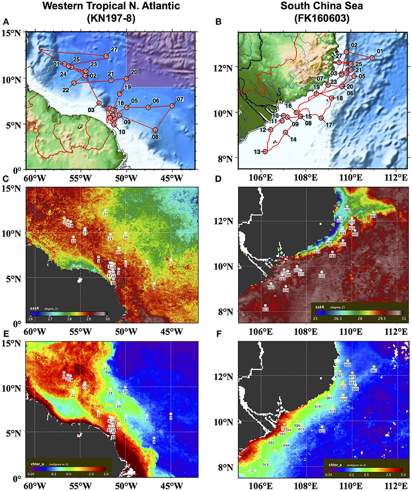
Figure 1. Station maps of (A) cruise KN197-8 in May–June 2010 in the Western Tropical North Atlantic (WTNA) off the coast of northern South America and (B) cruise FK160603 in June 2016 in the South China Sea (SCS) off the coast of Vietnam. Composite satellite images of MODIS-Aqua SST (C,D) and Chl a (E,F) for the month of June 2010 in the WTNA and for the month of June 2016 in the SCS, respectively. Note that the shaded inset at the top right of (A) corresponds to the area mapped in (B).

Comparison of Study Systems

Phytoplankton community structure in the WTNA is highly variable at small spatial and temporal scales due to the dynamic nature of the influence of the Amazon River plume. The Amazon River is the largest river in the world in terms of discharge, at peak flow delivering freshwater at a rate over 200 × 10³ m³s⁻¹ to the Atlantic Ocean (Geyer et al., 1996). As a result of its size, the river produces a large plume that can extend up to several thousand kilometers into the WTNA (Muller-Karger et al., 1995; Coles et al., 2013) and cover over a million square kilometers during the peak flow months between May and August (Subramaniam et al., 2008). Here, we apply the habitat type approach to data from a cruise during the peak flow season in May–June 2010, when the North Equatorial Current carried the Amazon River plume northward along the coast of South America (Figures 1A,C). The area investigated does not include the river mouth but includes extensive sampling of the sizeable offshore plume.

In the SCS, the phytoplankton community is influenced by the outflow of the Mekong River as well as seasonal coastal upwelling (Nguyen-Ngoc personal communication; Voss et al., 2006). This combination sets up sharp spatial and temporal gradients in physical and chemical properties. During the summer southwest monsoon (SWM) season, monsoonal rains intensify the outflow of the Mekong River, accounting for 85% of total annual discharge (Snidvongs and Teng, 2006), and local currents carry the river plume northward along the coast of Vietnam before it is deflected eastward at ~12°N by an offshore jet (Wu et al., 1998; Dippner et al., 2007). Between roughly 11° and 16°N, the SWM also drives coastal upwelling (Wyrtki, 1961; Xie et al., 2003). In our analysis, we used data from a cruise during the early SWM season in June 2016 (Figure 1B), the year after an El Niño Southern Oscillation (ENSO) event. ENSO events are known to cause a substantially weakened SWM (Chao et al., 1996; Zhang et al., 1996) and, in turn, low outflow of the Mekong River (Ha et al., 2018) and reduced coastal upwelling (Dippner et al., 2013). The timing of the cruise relative to both the SWM season and the 2015 ENSO event meant that the river outflow and upwelling were partially suppressed, though present and identifiable, during the sampling campaign (Figures 1D,F).

Materials and Methods

Generation of Habitat Types

Our general approach is to combine a principal component analysis (PCA) with a hierarchical cluster analysis to examine relationships among a defined set of environmental variables. The resulting analysis partitions the stations into statistically robust groups, which we call “habitats.” Our method is flexible and widely applicable, producing habitat types that reflect the biologically relevant physical and chemical drivers of each system to which it is applied. In order to make this approach both straightforward and general, we used the following criteria to identify environmental (or habitat-defining) variables:

1. Use variables that stem from common oceanographic measurements

2. Include biologically relevant variables that are sensitive to both physical and biological processes

3. Include both surface and upper water column properties that can be measured either directly or through proxies

4. Include both measurements that reflect instantaneous processes and others that integrate over time scales relevant to phytoplankton communities

A set of five variables together meet these criteria: sea surface temperature (SST) and salinity (SSS), mixed layer depth (MLD), depth of the chlorophyll a maximum (ChlMD), and nitrate availability to surface waters, which is represented here as a nitrate availability index (NAI). SST and SSS are properties that explicitly address the identity of surface waters, aiding in water mass identification and capturing the influence of water mass mixing. To extend this approach beyond classical water mass analyses, we also included three integrative parameters (MLD, ChlMD, and NAI) derived from vertical profiles.

We defined the MLD as the depth of the buoyancy frequency maximum, which reflects the location of maximum stratification and is particularly sensitive to gradients in water density. Among other things, MLD is sensitive to vertical advection from upwelling and the interaction of waters of varying density (e.g., a river plume spreading across marine waters). The thickness of the mixed layer is also relevant to phytoplankton as it governs their exposure to both light and nutrients.

The depth of the chlorophyll maximum (ChlMD) is an emergent ecosystem property influenced by multiple factors, including nutrient availability, light availability, and phytoplankton physiology and motility—all of which are modulated by hydrodynamics and food web interactions [summarized in Cullen (2015)]. In open ocean environments, the ChlMD generally occurs around the 1% light level and is an emergent property reflecting the interaction between nutrient availability from below and light availability from above. However, in upwelling systems and river plumes where nutrients are transported to the surface, the chlorophyll maximum may be at or near the surface.

Nutrient availability plays a critical role in shaping phytoplankton habitats. We focused on nitrate since nitrogen is often the limiting nutrient in coastal and oligotrophic marine ecosystems (Dugdale, 1967; Ryther and Dunstan, 1971; Falkowski, 1997; Howarth and Marino, 2006) and because of its role in regulating the abundance of diazotrophs.

One challenge in using nutrient concentration in our analysis is that surface concentrations of nitrate can vary from undetectable in offshore oligotrophic waters to several micromolar in areas affected by upwelling and river plumes. Although the nitracline depth can provide insight into nutrient availability in surface waters, the combination of coarse sampling, complex physical and chemical structure of profiles in dynamic systems, and the frequent occurrence of shallow water column depths creates real challenges in unambiguously defining the nitracline. To address this complexity, we developed an NAI as a proxy for nutrient availability in surface waters. NAI is defined as

$\text{NAI}=\left\{\begin{array}{ll}\left[{\text{NO}}_{2/3}\right],\hfill & \text{if }{\left[{\text{NO}}_{2/3}\right]}_{\text{surface}}\ge 0.5\text{μM}\hfill \\ -Z_{\left[{\text{NO}}_{2/3}\right]}=2\text{μM},\hfill & \text{if }{\left[{\text{NO}}_{2/3}\right]}_{\text{surface}}<0.5\text{μM}\hfill \\ -Z_{\text{bottom}},\hfill & \text{else}\hfill \end{array}\right\}$

where [NO_2/3] is the sum of the concentrations of nitrate and nitrite and Z is the water column depth, positive downward. This definition produces an index that scales directly with nutrient availability for surface phytoplankton. Specifically, positive NAI values reflect significant surface [NO_2/3], indicating a relief from nitrate limitation. In contrast, negative NAI values reflect a lack of nitrate at the surface, and NAI becomes increasingly negative as the depth of the nitracline increases in the absence of surface nitrate (see Figure S1).

The NAI cases, as well as the boundary values that define these cases, can be adjusted to fit the specifics of the system being analyzed. In this study, the Case 1 boundary value of 0.5 μM NO_2/3 was used because it is comparable to K_s values for nitrate uptake in marine phytoplankton and so will support appreciable rates of uptake (Eppley and Thomas, 1969). We used 2 μM NO_2/3 as the target value in Case 2 since it is high enough to be reliably interpolated in sparsely sampled profiles and provides a balance between registering influential features in the near surface and significant shifts in the nitracline.

Study Systems and Data Collection

The data presented here were obtained from two separate cruises: cruise KN197-8 was carried out in the WTNA aboard the R/V Knorr (22 May−25 June 2010; Figures 1A,C,E) and cruise FK160603 in SCS occurred aboard the R/V Falkor (3–19 June 2016; Figures 1B,D,F). On both cruises, we used Sea-Bird Electronics CTD-rosette systems equipped with fluorometers to measure the water column properties that form the basis of the habitat-defining variables. Samples for water column NO_2/3 concentrations were collected using Niskin bottles mounted on the CTD rosette and then measured using a Lachat QuikChem 8000 flow-injection analysis system. On cruise KN197-8, unfiltered nutrient samples were run immediately at sea. On cruise FK160603, nutrient samples were first filtered through 0.2 cellulose acetate filters and then frozen for analysis ashore.

On both cruises, every CTD cast with a measured nutrient profile was included in the habitat-type analysis, resulting in the analysis of 40 casts from 23 stations in the WTNA and 30 casts from 21 stations in the SCS. Each cast is identified by a “station.event” code (e.g., Figures 2C, 5C), where the digits to the left of the decimal are the station number and the digits to the right identify a specific sampling event at that station.

FIGURE 2

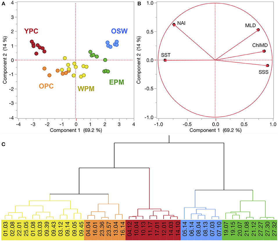
Figure 2. (A,B) Principal component analysis (PCA) of KN197-8 CTD casts from the WTNA based on the habitat-type defining variables (see text for explanation). The score plot (A) is a scatter plot of each cast's score according to the first two principal components, where colors correspond to habitat types. % variation explained by PC1 and PC2 is listed on their respective axes. The loading plot (B) shows the unrotated loading matrix between the analyzed variables and the first two principal components. The closer a variable's loading value is to 1, the greater the effect of the variable on that component. (C) Wards-mean hierarchical cluster analysis based on the habitat-defining variables. Habitat types are identified by color: young plume core (YPC), old plume core (OPC), western plume margin (WPM), eastern plume margin (EPM), and oceanic seawater (OSW).

Statistical Approach and Data Analysis

To generate the habitat types, we performed PCAs on covariances and hierarchical cluster analyses of the standardized habitat-defining variables (JMP Pro 14 software, SAS Institute Inc., Cary, USA). We tested for significant differences in variables among habitat types for both regions by performing one-way ANOVAs. All tests were significant (p < 0.0001); hence, we additionally ran post hoc Tukey–Kramer tests to identify significant differences among habitats (α = 0.05; Figures S2, S3).

Phytoplankton Community Structure

To test the utility of the habitat types, we compared them to surface measurements of phytoplankton community composition from the two cruises. In the WTNA, the community structure was delineated using a cluster diagram generated by Goes et al. (2014) on the Bray–Curtis dissimilarities of phytoplankton, which were determined fluorometically using an advanced laser fluorometer (ALF) during cruise KN197-8. Briefly, the ALF quantifies Chl a, chromophoric dissolved organic material (CDOM), and three classes of phycoerythrin (PE) pigments corresponding to blue water cyanobacteria (e.g., Trichodesmium spp. and Synechococcus spp.; PE-1), green water cyanobacteria (e.g., DDA symbionts; PE-2), and cryptophytes common in fresh and brackish waters (PE-3; Chekalyuk and Hafez, 2008; Chekalyuk et al., 2012).

For the SCS, we assessed surface phytoplankton communities using both diagnostic phytoplankton pigments and microscopic cell counts. Phytoplankton pigments were measured and analyzed using high-performance liquid chromatography as described in Van Heukelem and Thomas (2001). One to two liters of water collected from the surface using the CTD rosette was filtered through a GF/F filter. The filters were frozen in liquid nitrogen until analysis. Seven pigment classes were evaluated in this study: divinyl chlorophyll a + b (DvChla+b) was used as a proxy for prochlorophytes, 19′ butanoyloxyfucoxanthin (19′BF) was used for pelagophytes and haptophytes, 19′ hexanoyloxyfucoxanthin (19′HF) was used for haptophytes, alloxanthin (Allo) was used for cryptophytes, zeaxanthin (Zea) was used for cyanobacteria, peridinin (Peri) was used for dinoflagellates, and fucoxanthin (Fuco) was used for diatoms [according to Jeffrey et al. (1997) and Vidussi et al. (2001) and references therein].

Direct cell counts were drawn from Doan-Nhu (unpublished data) and are plotted here for comparison with the habitat-type analysis. Our analysis includes 135 species or groups of phytoplankton collected from the top 5 m of the water column.

Both the SCS pigment and cell count datasets were analyzed statistically to assess how well the habitat type groupings are reflected in the phytoplankton communities. The following analyses were done using PRIMER-6 with PERMANOVA+ add-on software (Primer-E Ltd., Plymouth, UK). We first generated resemblance matrices of both datasets: for the pigment data, we generated chi-squared distances in order to mitigate the effect of large-scale differences between habitats (e.g., Faith et al., 1987); for the species-specific cell counts, we followed the classical approach of generating Bray–Curtis dissimilarities on log(x + 1)-transformed abundances. A PERMANOVA was then performed on the resemblance matrices of both datasets to test for significant differences in phytoplankton communities between habitat types. Since both tests were significant (p < 0.001), a canonical analysis of principal coordinates (CAP) was then performed. CAP is a constrained ordination technique that maximizes the explained variance between a priori groups and estimates error rates using leave-one-out cross-validation (Anderson and Robinson, 2003; Anderson and Willis, 2003). Canonical correlations are based on 999 permutations (p < 0.001 for both analyses). The individual pigments or species that are likely responsible for the observed differences between habitats were identified using the Pearson correlations of the pigment concentrations and cell abundances with their respective canonical axes. The correlations were calculated on the standardized pigment concentrations and on the untransformed cell abundances.

Results

The habitat-type approach produced appreciable separation of stations from both the WTNA and SCS systems into distinct habitat types.

Habitats in the Western Tropical North Atlantic

In the WTNA, the first two principal components of the PCA described a total of 83.2% of the overall variation in the system (Figure 2). PC1 alone accounted for 69.2% and was driven rather strongly by SST, SSS, and ChlMD. NAI and MLD contributed roughly equally to both PCs, but were the primary drivers of PC2, which accounted for 14.0% of the total variation.

The combination of the PCA and cluster analysis generated five habitat types (Figure 2), which we have termed young plume core (YPC), old plume core (OPC), western plume margin (WPM), eastern plume margin (EPM), and oceanic seawater (OSW), names that reflect general habitat locations (Figure 3A) and properties. The PCA (Figure 2) and summary of environmental variables by habitat type (Table 1, Figure S2) indicate that the habitat types are arrayed along a continuum of the habitat-defining variables, with the nearshore Amazon River water (YPC) at one extreme and oceanic waters (OSW) at the other. Along this continuum, SST decreases whereas SSS, MLD, and ChlMD all increase. In contrast, NAI is similar across all but the YPC habitat, where nitrate availability is much higher due to rather shallow nitraclines. Note that nitrate availability is important in differentiating the YPC and OPC habitat types.

FIGURE 3

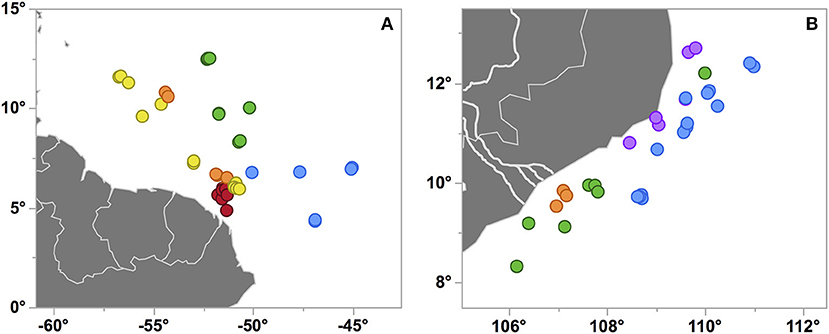
Figure 3. Station maps of cruises KN197-8 in the WTNA (A) and FK160603 in the SCS (B) where each marker corresponds to a CTD cast. Markers are colored by habitat types as in Figures 2, 5, respectively, and are slightly jittered to reveal some of the overlapping markers. The Mekong River in panel (B) is represented by the bold white lines.

TABLE 1

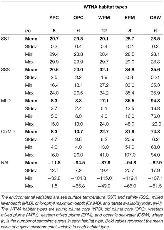
Table 1. Summary of environmental variables used to define habitat types in the Western Tropical North Atlantic (WTNA).

The WTNA habitat types are largely distinct geographically (Figure 3A), with YPC nearest the river mouth and OSW offshore to the east and well out of the path of the river plume. OPC and WPM habitats overlap geographically and in PCA space, though OPC is distinct from WPM based on its much fresher surface waters (Figure S2). The EPM habitat is located farther offshore and to the east of the OPC and WPM habitats. EPM waters are generally similar to OSW except for EPM's much shallower MLDs.

Relating Habitats to Phytoplankton Communities in the Western Tropical North Atlantic

To explore the biological relevance of the habitat types, we compared our habitat divisions to the surface phytoplankton populations characterized by Goes et al. (2014), who evaluated community diversity using a cluster analysis of ALF fluorescence measurements. They then overlaid SSS-based “water-type” categories onto their cluster diagram, where oceanic (OC) waters had SSS > 35, coastal mesopelagic (CM) had SSS between 30 and 35, and estuarine (ES) had SSS < 28 (see our modified version as Figure 4, where we have also relabeled Stn 21 as “CM” instead of “OC” based on its SSS).

FIGURE 4

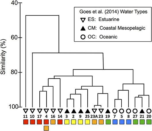
Figure 4. Modified dendrogram from Goes et al. (2014) based on the Bray–Curtis similarities of ALF fluorescence data measured on surface station samples from KN197-8. The water types defined by Goes et al. (2014) are shown with the black and white symbols and are labeled with the station number. Below the station labels, we have added colored squares corresponding to our habitat-type categorizations in Figure 2.

We compared our habitat-type divisions to the cluster diagram and SSS-based water types of Goes et al. (2014) by placing colored markers corresponding to our habitat types below a replotted version of their dendrogram (Figure 4). This visual comparison shows that our habitat types correspond quite well to both the dendrogram and the water types of Goes et al. (2014). For example, our WPM (yellow) habitat matches very well with the primary “CM” cluster. There are, however, a few important differences: The habitat-type definition produces finer distinctions in the Goes et al. (2014) “OC” waters. These distinctions are also reflected in the dendrogram itself, where OC waters are divided between our EPM (green) and OSW (blue) habitat types. The habitat-type analysis additionally did a better job of classifying Stn 21 according to its phytoplankton community, as evidenced by the dendrogram clustering (Figure 2C). Conversely, the habitat-type analysis differentiates stations in the lower-salinity, more plume-influenced region in a way that is not obviously supported by the dendrogram.

Habitats in the South China Sea

The region sampled in the SCS exhibited a similar degree of habitat-type separation. The first two PCs explained 86.8% of the variance, where PC1 explained 54.3% and was primarily driven by the emergent properties MLD, ChlMD, and NAI (Figure 5). PC2 captured 32.5% of the variation and was driven primarily by the surface properties of SST and SSS. Combined, the PCA and cluster analysis generated four habitat types, which we have termed Mekong River water (MRW), onshore or continental shelf waters (OnSW), upwelled waters (UpW), and OSW based on their properties and locations. PC1 accounted for most of the separation between MRW, OnSW, and OSW habitats, whereas PC2 was important in distinguishing UpW from OnSW and MRW habitats.

FIGURE 5

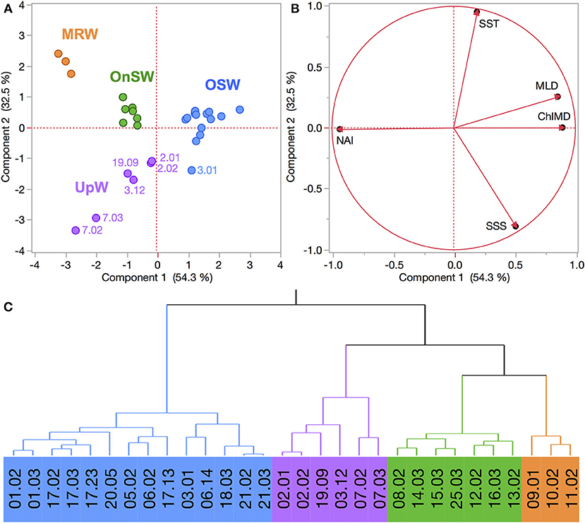
Figure 5. (A,B) PCA of FK160603 CTD casts from the SCS based on the habitat-type defining variables. See Figure 2 for explanation of plots. (C) Wards-mean hierarchical cluster analysis based on the habitat-defining variables. Habitat types are identified by color: Mekong River water (MRW), on-shelf water (OnSW), upwelled water (UpW), and oceanic seawater (OSW).

Altogether MRW stations were located near the mouth of the Mekong River (Figure 3B) and were characterized by the combination of shallow MLDs and Chl a maxima, high NAI, and fresh, warm surface waters (Table 2, Figure S3). In contrast, OSW stations were located farther offshore and had the deepest MLDs and Chl a maxima, the lowest NAI, and SST and SSS typical of surface oceanic waters in the region. UpW stations varied in their properties, but had generally shallow MLDs and ChlMDs, higher nutrient availability than OSW stations, but were saltier and cooler at the surface than either MRW or OnSW waters. These stations were located along the northern coast of our sampling area, consistent with the typical location of the monsoon upwelling. The OnSW stations, like those belonging to OSW, appear to have been minimally influenced by either the Mekong River or upwelled waters, but were located near shore and had shallower MLDs, ChlMDs, and nitraclines than OSW.

TABLE 2

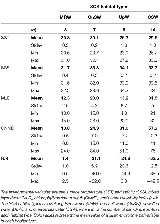
Table 2. Summary of environmental variables used to define habitat types in the South China Sea (SCS).

Relating Habitats to Phytoplankton Communities in the South China Sea

We used two metrics of community composition, diagnostic pigments and species-specific cell counts, to assess the relevance of our habitat types to the surface phytoplankton communities. Using CAP, this is achieved both visually with ordination plots and through error analysis with cross-validation. The ordination plots of both community metrics (Figures 6A,B) reveal appreciable separation of the habitat types, particularly between the MRW, OnSW, and OSW habitats, whereas the UpW habitat is less well defined. In both analyses, CAP 1 primarily separated MRW from OnSW and OSW (correlation coefficients of δ² = 0.81 and 0.94 for pigments and cell counts, respectively), whereas CAP 2 chiefly separated OnSW from MRW and OSW (δ² = 0.75 and 0.73, respectively).

FIGURE 6

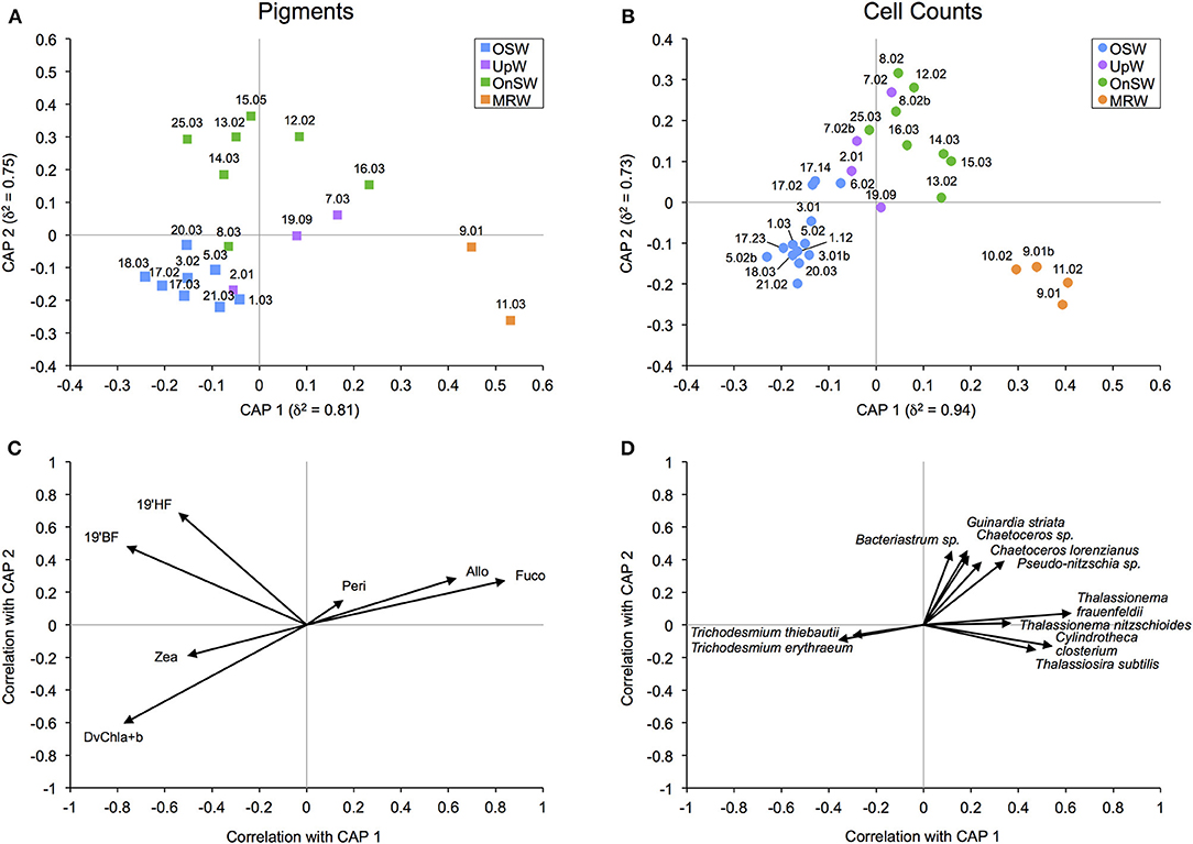
Figure 6. Canonical analysis of principal coordinates (CAP) ordination for diagnostic pigment (A) and species-specific cell count (B) community data. δ² is the canonical correlation of a given axis. The biplots display the correlations of phytoplankton pigments (C) and species (D) with their respective canonical axes. The species plot (D) shows only the phytoplankton with a Pearson correlation of |r| ≥ 0.3 that also comprised ≥2% of the total abundance of the habitat with which they best correlate. For example, the four species correlating most strongly and positively with CAP 1 made up ≥2% of the abundance sampled at the four MRW casts. Given the poor separation of UpW from OSW and OnSW habitats (see also Table 3), UpW was not explicitly considered in the abundance calculations.

Cross-validation supports the ordination results given the 80% success rate by the analysis to correctly classify pigment samples into their predetermined habitat types and the 72.4% success rate for cell count samples (Table 3). The majority of the error in both analyses derived from the UpW habitat, with only 33.3 and 25% of samples from this habitat correctly assigned for the pigment and cell count datasets, respectively. On closer inspection, there were distinct differences between the habitat-type classification and the phytoplankton communities found at Stns 2, 7, and 14 (Table 4). Pigment and cell count samples from Stns 2 and 14 derived from the same CTD casts and were misclassified consistently: the habitat-type analysis classified cast 2.01 as UpW and cast 14.03 as OnSW, whereas the phytoplankton communities as defined by both pigments and cell counts indicated that the casts belonged to OSW and UpW, respectively.

TABLE 3

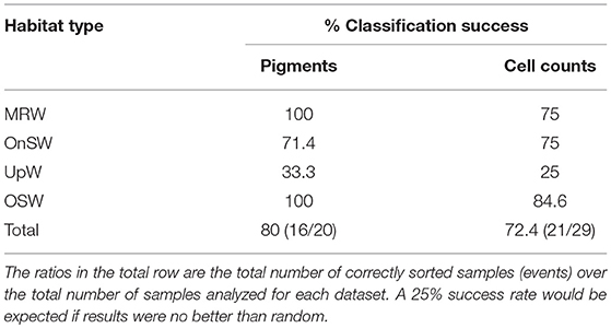
Table 3. Classification success of pigment and cell count community samples to their predefined habitat types.

TABLE 4

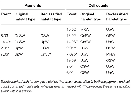
Table 4. Events that were misclassified during the canonical analysis of principal coordinates (CAP) cross-validation routine.

The biplot of the diagnostic pigments (Figure 6C) indicates that DvChla+b and Zea correlated negatively with both CAP 1 and 2, whereas 19′BF and 19′HF correlated negatively with CAP 1 but positively with CAP 2. Fuco, Allo, and, to some extent, Peri correlated positively with both axes. For the species biplot (Figure 6D), only the most prominent species in terms of correlation strength and abundance are shown for clarity. Two species of the cyanobacteria Trichodesmium correlated negatively with primarily CAP 1, whereas the diatoms Thalassiosira subtilis, Cylindrotheca closterium, and two species of Thalassionema correlated positively. The remaining five phytoplankton, all of which are diatoms (Bacteriastrum sp., Guinardia striata, Chaetoceros sp., Chaetoceros lorenzianus, and Pseudo-nitzschia sp.), correlated roughly equally and positively with CAP 1 and 2.

Discussion

Our goal with the habitat-type analysis was to use an integrative method to complement and extend a purely physical approach for evaluating dynamic marine regions and to gain insights into the biogeography and community structure of phytoplankton in these regions. Our method partitions habitat space using biologically relevant environmental variables that integrate over varying time and space scales. We have applied this method to regions in the WTNA and SCS that differ substantially in their scale, nutrient sources/sinks, and hydrographic complexity, providing a robust test of the applicability of our concept.

Despite the significant differences between our two systems, our approach performed very well in both cases. The first two principal components in our PCAs using the five habitat-defining variables accounted for 83.2 and 86.8% of total system variances in the WTNA and SCS, respectively (Figures 2, 5). Interestingly, the five variables contributed roughly equally to the total explained variance of the first two PCs in both cases, as indicated by the variable loadings in Figures 2B, 5B. These results demonstrate that our variable set is comprehensive and that all variables are highly relevant to both the WTNA and SCS systems.

Importantly, the habitat-type analysis also partitioned the CTD casts from each cruise into coherent habitats, though the divisions of these habitats reflect different drivers of physical and chemical variability within the two systems.

Habitats in the Western Tropical North Atlantic

In the WTNA, the sampled region is effectively a two-end-member system defined by mixing of the Amazon River plume with oceanic waters. The resulting habitat types defined by the analysis form a continuum of river water age and mixing history. As described previously (Goes et al., 2014; Weber et al., 2017), the fresh/warm “core” of the plume extending northwest into the research area can easily be identified using salinity alone. Two of the defined habitats fall within the core plume, where a sharp drop in surface nitrate availability (NAI) distinguishes the YPC from the older plume core (OPC) waters (Table 1, Figure S2).

Farther offshore, the habitat analysis clearly delineated regions west and east of the plume axis, which we accordingly termed WPM and EPM. In the overall physical and biogeochemical context of the WTNA, our habitats show a clear trend of decreasing river plume influence from the plume core (YPC and OPC) to WPM to EPM to OSW habitats, where OSW conditions reflect the surrounding oligotrophic waters in the region.

Relative to OSW, greater direct inputs of plume water or more frequent exposure to plume filaments will increase SST, reduce SSS, and cause prominent shoaling in the MLD (as at WPM stations). The depth of the chlorophyll maximum (ChlMD) will also be shallower due to a combination of fertilization within the near-surface plume and sustained shading of deeper waters, limiting the formation of a deeper chlorophyll maximum (Lu et al., 2010). Where river plume exposure is less intense or frequent, SST and SSS may be only slightly different from oceanic values. The MLD and ChlMD, however, may respond differently under these conditions: whereas the MLD is sensitive to even weak plume infringement, the ChlMD is a time-integrative property dependent on both phytoplankton biomass (Cullen, 2015 and references therein) and physiology (Steele, 1964; Fennel and Boss, 2003). In consequence, changes in a variable such as irradiance may not have an immediate effect on either the position or intensity of ChlMD.

In practical terms for the WTNA, this means that weak exposure to the surface river plume (in terms of either intensity or duration) may not appreciably affect ChlMD (e.g., in the EPM habitat), whereas extended presence of a surface plume will attenuate light strongly enough and long enough to alter the ChlMD (e.g., in the WPM habitat). The environmental variables thus indicate that the EPM habitat experienced less intense/frequent plume influence than the WPM habitat. More generally, this contrast demonstrates how a consideration of environmental variables with differing sensitivities and characteristic time scales can elucidate causes of regional habitat variability.

Relating Habitats to Phytoplankton Communities in the Western Tropical North Atlantic

To continue our assessment of the applicability of our habitat analysis, we compared our results to those of a previous study that fluorometrically characterized the phytoplankton communities from this same cruise (Goes et al., 2014). Through this comparison, we find that our habitat types correlate quite well with their SSS-based water-type groupings and with their fluorescence-based cluster diagram of community composition (Figure 4), particularly for the more offshore stations. With the exception of Stn 19, the EPM and OSW habitats fall neatly within a single cluster but revealed a finer distinction in the ALF community data since these habitats map onto two distinct subclusters within the “OC” water type of Goes et al. (2014). The EPM habitat is distinguished from OSW based on its slightly warmer/fresher surface waters and significantly shallower MLDs, indicative of more recent river plume influence and greater nutrient availability. Although the signal of the offshore plume is rather weak in these waters (compared to WPM), the cluster division between EPM and OSW suggests that even a weak influence of the aged offshore plume is enough to modify surface phytoplankton communities.

Interestingly, the comparison revealed little biological distinction between the young (YPC, red) and old (OPC, orange) plume core habitats, suggesting that nitrate availability (NAI), the primary distinguishing variable between YPC and OPC habitats (Figure 2), is not a critical factor shaping these communities. Even though nitrate is not present in surface waters at the OPC stations, the plume phytoplankton communities may be sustained through regenerated production, which can be significant in offshore plumes of large rivers (Wawrik et al., 2004). Station 4 within this same cluster provides an additional example of the high variability in this river plume system. During 7.5 h of sampling at this location, the upper water column changed enough to drive a shift in habitat type from OPC to YPC. Such rapid changes in physical and chemical conditions are likely due to advection and illustrate the inherent challenges in working in such environments.

The habitat types generated by our approach are clearly biologically relevant and can provide insights into the spatial and temporal coupling between environmental drivers and the response of the phytoplankton community. Specifically, the phytoplankton community characteristic of each habitat type must have time to grow in, and phytoplankton community composition will always lag behind shifts in environmental conditions. As a result, mismatches between the phytoplankton community and habitat type at a station can provide a tool for identifying recent and/or rapid changes in the physical and chemical environment.

Finally, this approach can be used to generate hypotheses about the phytoplankton community type at stations where the variables needed for habitat classification are available but direct measurements of the phytoplankton community are lacking. That is, our approach can help fill gaps in phytoplankton datasets by placing spatially and temporally sparse biological information in a larger, more robust set of physical and chemical measurements. The WTNA dataset includes five casts from five stations (Stns 1, 6, 12, 13, and 22) that were included in our habitat analysis, but which lacked ALF data, making them ideal for an assessment of the potential use of this analysis in predicting phytoplankton communities (Figure 4). We used a natural breakpoint in the ALF dendrogram to group the casts with ALF data into phytoplankton community groups (signified by the cluster color in Figure 7A) and then mapped these community groups onto corresponding casts in the habitat-type PCA (Figure 7B). In Figure 7B, the habitat types are distinguished from the community groups based on the colors of marker borders and fillings: border color corresponds to the habitat type and filling color corresponds to the ALF-based phytoplankton community group. As such, the five casts without ALF data have markers with border colors matching their habitat types, but they lack filling since they were not in the dendrogram. Our approach reveals good general agreement between the ALF groupings and our habitat types. Specifically, four of the five test casts fall neatly into regions where the two categorizations agree, implying that the habitat types we assigned provide an indication of the phytoplankton communities likely to be found at these stations. The one case where the habitat types did not map definitively onto a single ALF-based community (Station 12) reflects a mismatch between the resolution of ALF groupings and habitat types within the plume core waters.

FIGURE 7

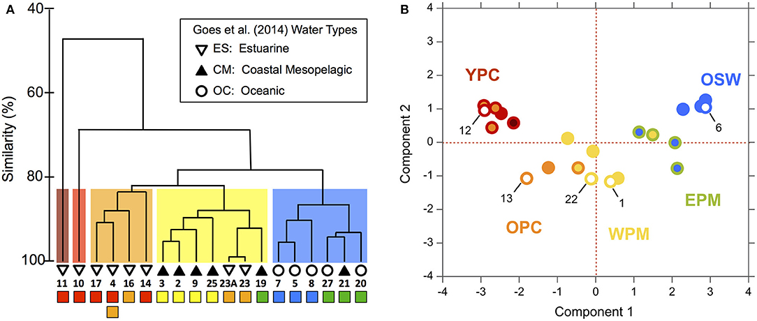
Figure 7. (A) Dendrogram of ALF data from Goes et al. (2014) where clusters have been grouped at ~83% similarity according to the colored boxes behind the clusters and are referred to as “cluster groupings” in the main text. The colored squares below the station numbers correspond to our habitat-type categorizations. See Figure 4 for additional information. (B) PCA of habitat-defining variables from Figure 2 comparing the ALF cluster groupings to the habitat types, where the marker border color has been kept the same so as to match habitat types, whereas the marker fill color was changed to match that of the ALF cluster groupings (A). Markers filled with white represent CTD casts from stations that had no corresponding ALF dataset. Only one CTD cast per station is shown (see section Materials and Methods); note that the marker of Station 25 is nearly fully eclipsed by that of Station 22.

Habitats in the South China Sea

The habitat-type analysis for the SCS dataset also achieved a high degree of separation among habitats, which largely reflect the three primary end members in the sampling area: the Mekong River (MRW), coastal upwelling (UpW), and oceanic waters (OSW). The fourth habitat type, OnSW, is not an end member per se but is composed of shelf waters that are transported from the Gulf of Thailand and mixed in differing proportions with the other three end members (Dippner and Loick-Wilde, 2011). The dynamic nature of this system is seen in the high degree of spatial and temporal variability, including significant changes in the physical properties of the water column at short scales (h/km). Thus, in the discussion below, we focus on individual CTD casts rather than using stations, since properties could change significantly between repeated samplings at a geographic location.

Both the Mekong River and coastal upwelling were geographically restricted but clearly discernable in the region (Figures 3, 5), with limited expressions that likely reflect the combination of the post-ENSO (Dippner et al., 2013; Ha et al., 2018) and early-season SWM timing of our cruise. Whereas the influence of the Mekong River was rather coherent across the affected stations, the expression of upwelling was both patchy and variable in the PCA space, as seen in the distribution of the UpW CTD casts within the PCA score plot (Figure 5A). In combination with the vectors mapped in the loading plot (Figure 5B), the relative positions of the casts in the PCA score plot reflect the environmental variables driving the casts' distributions. The UpW subgroup farthest from the other casts (corresponding to two casts from Stn 7) has the strongest upwelling signal from the youngest/least altered upwelled waters sampled (coolest SST and shallowest MLD and ChlMD). The remaining UpW casts (Stns 2, 3, and 19) extend toward the center of the PCA plot with properties more similar to those of OSW and OnSW stations. This pattern suggests that the upwelled waters at these stations are characterized by relatively greater age/mixing compared to Station 7.

In addition to geographic heterogeneity, we also see clear evidence of temporal variability in the expression of upwelling. At Station 3, two casts (3.01 and 3.12) sampled within 9 h and 1 km of one another were classified into different habitat types (Figure 5). Cast 3.01 is an edge case whose properties place it uniquely on the border between OSW and UpW habitats (Figure 5A). The SST and SSS of both casts are nearly identical and indicative of aged/altered upwelled water, whereas all of the integrated properties differ such that cast 3.01 is more similar to OSW waters (deeper MLD and ChlMD and a negative NAI).

Relating Habitats to Phytoplankton Communities in the South China Sea

We can now assess the relevance of these habitats to surface phytoplankton distributions. For the SCS, we have both diagnostic pigments and species-specific cell counts, which provide complementary measures of phytoplankton community composition. Diagnostic pigments offer a coarser assessment of community composition in terms of higher taxonomic groups (Vidussi et al., 2001). Though some of the diagnostic pigments occur in multiple groups of phytoplankton [e.g., Zeaxanthin, indicative of cyanobacteria, is also a common photo-protectant in eukaryotic phytoplankton (Kana et al., 1988)], they offer a broad overview of community composition that importantly includes prochlorophytes (DvChla+b), which are notoriously difficult to quantify with traditional microscopy. Complementing this high-level assessment, microscopy-based cell counts provide an extremely detailed view of the larger (>2 μm) phytoplankton community.

Despite their differences in resolution and coverage, these two community metrics had strikingly similar CAP results, both of which showed that the habitat-type groupings were largely relevant to the phytoplankton communities. Both metrics showed particularly clear contrasts among the MRW, OnSW, and OSW habitats. The community of the UpW habitat, however, did not show a clean separation from the OnSW and OSW communities (Figures 6A,B) and consequently had very poor classification success rates (Tables 3, 4), with that of the cell count analysis no better than random. These results indicate that there is no single, distinct UpW community, though this is not altogether surprising since we know from the habitat analysis that there is considerable heterogeneity in the expression of upwelling at UpW stations (Figure 5A) and that the upwelling signal itself was fairly weak at the time of sampling. As a result, the lag between changing environmental conditions and phytoplankton community responses likely prevented the development of a characteristic UpW community.

The high error rates associated with the UpW habitat due to a lack of a coherent community make it difficult to draw definitive conclusions about the specific events that were misclassified during cross-validation, particularly those that were reclassified as UpW. We do note, however, that some of the same UpW stations were misclassified in both datasets (Table 4). For example, Stn 2.01, which was consistently reclassified as OSW, was also the most OSW-like out of the UpW casts in the habitat analysis (Figure 5A). It is plausible that at this station, the upwelling was so weak and/or recent that the resulting changes in the physical/chemical conditions of the waters had not significantly altered the (already-present) oceanic phytoplankton community. Similarly, we may see evidence of lags in community response to changing conditions at Stns 8.03 and 13.02, where the habitat-type analysis classified them as OnSW but their phytoplankton communities are more similar to that of OSW communities (Table 4).

CAP easily separated the remaining three habitats, of which MRW and OSW received the highest classification success rates (Figures 6A,B, Table 3). Unlike OnSW, these two habitats reflect distinct end members in the SCS, and phytoplankton in these waters likely experience stronger or more consistent selective pressures on the basis of nutrient availability (among other things). For example, according to our NAI, the OSW surface waters are very limited in nitrate. The biplots identified two groups of phytoplankton that correlated strongly with these nitrate-limited OSW waters: prochlorophytes (DvChla+b; Figure 6C) and Trichodesmium spp. (Figure 6D)—both of which contain Zea. These phytoplankton, which are known to thrive in “blue” waters, possess adaptations for oligotrophic conditions (e.g., large surface-area-to-volume ratio and the ability to fix N₂, respectively), making them well suited to the OSW habitat.

Conversely, species with a broader salinity-range tolerance and that are well adapted to nutrient-replete environs correlated with the MRW habitat (e.g., Thalassionema spp., Cy. closterium, and Thalassiosira subtilis; Figure 6D). Though MRW phytoplankton formed their own distinct communities, they also shared many similarities with the OnSW communities (e.g., Thalassionema spp.; Figure 6D), likely due to the higher nutrient availability that often occurs in coastal waters. This is also seen in a broader sense with the pigment biplot, where diatoms (Fuco) and cryptophytes (Allo) appear to correlate strongly with both habitats (Figures 6A,C). Despite these commonalities, there were a handful of neritic species common to the SCS [summarized in Voss et al. (2014)] that were particularly abundant in the OnSW waters, including Bacteriastrum sp., G. striata, Chaetoceros spp., and Pseudo-nitzschia sp. (Figures 6B,D). Importantly, these results in particular and those of the CAP analyses in general further support distinguishing the OnSW waters as a distinct habitat, even though it represents a mix of the system's end members.

Somewhat similar to the situation in the WTNA, we can use our statistically significant habitat types as an aid to frame hypotheses about the habitat type and phytoplankton community structure when some of the necessary data are missing. In the case for the SCS, there are three casts (Stns 23.02, 23.03, and 27.01) that had to be excluded from the habitat analysis due to a lack of nutrient data necessary to calculate NAI. At both of these stations, samples for phytoplankton cell counts were collected, and at Stn 23, pigment samples were also gathered. Since the habitat types were shown to be statistically significant with CAP, we can use their phytoplankton communities to infer their habitat types.

Using the sample add-in routine (in PRIMER), the samples were placed in ordination space and their distance to the nearest habitat-type centroid was used to determine their likely habitat. The routine placed the casts from Stn 23 closest to the OnSW centroid in both analyses (Figures 8A,B), whereas Stn 27.01 was placed nearest the UpW centroid in the cell count analysis (Figure 8B). The consistency between both add-in routines for Stn 23 is encouraging, though the result is somewhat surprising given that the other available environmental data place it neatly into the OSW habitat (SST: 30.2°C, SSS: 33.5°C, MLD: 42 m, ChlMD: 48 m). This may reflect a transition from OnSW to OSW, meaning that even though the waters physically and chemically look oceanic, species like Trichodesmium spp. have not yet grown in.

FIGURE 8

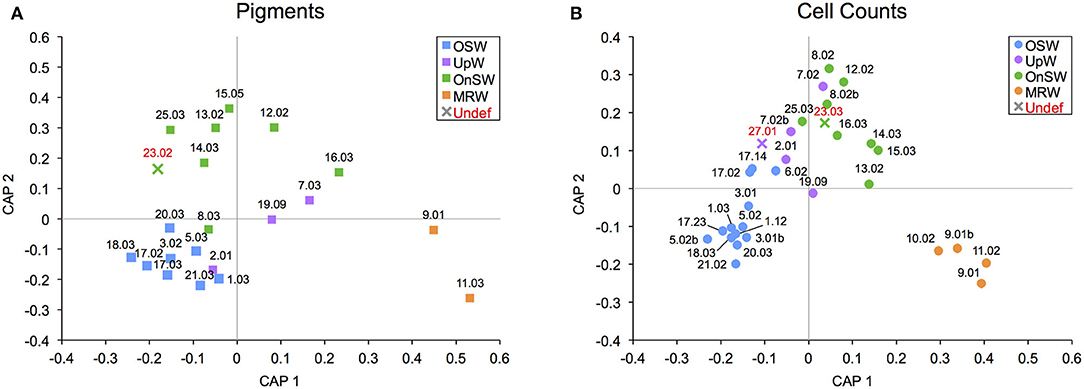
Figure 8. Addition of samples with undefined habitat types into canonical analysis of principal coordinates (CAP) ordination plots for diagnostic pigment (A) and species-specific cell count (B) community data. Samples that were added are labeled in red, and their marker color matches that of the closest habitat.

As for Stn 27.01, despite the high classification error rates for this UpW habitat (Table 3), this result is consistent with the proximity of the station to the northern coastline where upwelling was observed (Figure 1D) and with the environmental data we do have (SST: 25.9°C, SSS: 34.3°C, MLD: 5 m, ChlMD: 47 m), which would place Stn 27.01 well within the UpW habitat.

Conclusions

In this manuscript, we have demonstrated a straightforward and powerful approach for interpreting and understanding environmental and biological datasets in highly variable marine environments. In essence, we generated a framework for evaluating phytoplankton communities based on five biologically relevant and commonly measured environmental variables. These variables are derived from standard oceanographic measurements that span both conservative and emergent properties of a system, meaning that this approach is both simple to implement and widely applicable.

We have tested this approach on two systems of very different size and end member complexity. For both systems, the analysis generated statistically robust habitat classifications that were largely relevant to surface phytoplankton communities. A more careful analysis of the habitat-defining variables themselves led to insights into the processes acting on the systems and shaping phytoplankton communities within them. For example, by evaluating variables that are differentially sensitive and that integrate over varying time scales, it is possible to infer the frequency/intensity of major system forcings. In addition, situations where the local phytoplankton community is atypical for the derived habitat type can result from a mismatch between the rates of change in physical and chemical characteristics of the water and the phytoplankton community response, providing a marker of recent change in the system. Overall, our habitat types captured the major patterns of phytoplankton distribution in two complex ocean margin systems regardless of how community composition was measured.

Data Availability

The datasets generated for this study are available on request to the corresponding author.

Author Contributions

SW, AS, and JM conceived and designed the research. All authors contributed to the collection and compilation of data. SW, AS, JM, and HD-N analyzed the data. SW, AS, and JM wrote the manuscript. All authors contributed to content revisions and approved the final text.

Funding

SW and MV were supported by the German Research Foundation grant DFG VO 487/13-1. AS was supported by the Gordon and Betty Moore Foundation grant #4886, NASA grant NNX16AJ08G, and National Science Foundation grant NSF-OCE-1737128. HD-N, LN-N, and SW were supported by the National Foundation for Science and Technology Development (NAFOSTED) grant DFG 106-NN.06-2016.78. SW and JM were supported by grant NSF-ETBC-0934025. JM was supported by grant NSF-OCE-1737078. Shiptime in the South China Sea was supported by a grant from the Schmidt Ocean Institute. LDEO contribution #8282.

Conflict of Interest Statement

The authors declare that the research was conducted in the absence of any commercial or financial relationships that could be construed as a potential conflict of interest.

Acknowledgments

We thank the officers and crew of the R/V Knorr and R/V Falkor for their help and support at sea. We also thank Dr. Natalie Loick-Wilde for her constructive feedback, Ms. Nguyen Thi Mai Anh for her technical assistance with the SCS phytoplankton data, and two reviewers for their comments and helpful suggestions.

Supplementary Material

The Supplementary Material for this article can be found online at: https://www.frontiersin.org/articles/10.3389/fmars.2019.00112/full#supplementary-material

Abbreviations

19′BF, 19′ butanoyloxyfucoxanthin; 19′HF, 19′ hexanoyloxyfucoxanthin; ALF, advanced laser fluorometer; Allo, alloxanthin; CAP, canonical analysis of principal coordinates; CDOM, chromophoric dissolved organic material; ChlMD, chlorophyll maximum depth; CM, coastal mesopelagic; CTD, conductivity temperature depth; DDA, diatom diazotroph associations; DvChla+b, divinyl chlorophyll a + b; ENSO, El Niño Southern Oscillation; EPM, eastern plume margin; ES, estuarine; Fuco, fucoxanthin; MLD, mixed layer depth; MRW, Mekong River water; NAI, nitrogen assimilation index; NO2/3, nitrate + nitrite; OC, oceanic; OnSW, onshore seawater; OPC, old plume core; OSW, oceanic seawater; PC, principal component; PCA, principal component analysis; PE, phycoerythrin; Peri, peridinin; SCS, South China Sea; SSS, sea surface salinity; SST, sea surface temperature; SWM, southwest monsoon; UpW, upwelled water; WPM, western plume margin; WTNA, Western Tropical North Atlantic; YPC, young plume core; Zea, zeaxanthin.

References

Anderson, M. J., and Robinson, J. (2003). Generalized discriminant analysis based on distances. Aust. N.Z. J. Stat. 45, 301–318. doi: 10.1111/1467-842X.00285

CrossRef Full Text | Google Scholar

Anderson, M. J., and Willis, T. J. (2003). Canonical analysis of principal coordinates: a useful method of constrained ordination for ecology. Ecology 84, 511–525. doi: 10.1890/0012-9658(2003)084[0511:CAOPCA]2.0.CO;2

CrossRef Full Text | Google Scholar

Chao, S-Y., Shaw, P-T., and Wu, S. Y. (1996). El Niño modulation of the South China Sea circulation. Progr. Oceanogr. 38, 51–93. doi: 10.1016/S0079-6611(96)00010-9

CrossRef Full Text | Google Scholar

Chekalyuk, A., and Hafez, M. (2008). Advanced laser fluorometry of natural aquatic environments. Limnol. Oceanogr. Methods 6, 591–609. doi: 10.4319/lom.2008.6.591

CrossRef Full Text | Google Scholar

Chekalyuk, A. M., Landry, M. R., Goericke, R., Taylor, A. G., and Hafez, M. A. (2012). Laser fluorescence analysis of phytoplankton across a frontal zone in the California Current ecosystem. J. Plankton Res. 34, 761–777. doi: 10.1093/plankt/fbs034

CrossRef Full Text | Google Scholar

Coles, V. J., Brooks, M. T., Hopkins, J., Stukel, M. R., Yager, P. L., and Hood, R. R. (2013). The pathways and properties of the Amazon River Plume in the tropical North Atlantic Ocean. J. Geophys. Res. Oceans 118, 6894–6913. doi: 10.1002/2013JC008981

CrossRef Full Text | Google Scholar

Cullen, J. J. (2015). Subsurface chlorophyll maximum layers: enduring enigma or mystery solved? Ann. Rev. Mar. Sci. 7, 207–239. doi: 10.1146/annurev-marine-010213-135111

CrossRef Full Text | Google Scholar

DeMaster, D. J., Smith, W. O., Nelson, D. M., and Aller, J. Y. (1996). Biogeochemical processes in Amazon shelf waters: chemical distributions and uptake rates of silicon, carbon and nitrogen. Cont. Shelf Res. 16, 617–643. doi: 10.1016/0278-4343(95)00048-8

CrossRef Full Text | Google Scholar

Dippner, J. W., Bombar, D., Loick-Wilde, N., Voss, M., and Subramaniam, A. (2013). Comment on “Current separation and upwelling over the southeast shelf of Vietnam in the South China Sea” by Chen et al. J. Geophys. Res. Oceans 118, 1618–1623. doi: 10.1002/jgrc.20118

CrossRef Full Text | Google Scholar

Dippner, J. W., and Loick-Wilde, N. (2011). A redefinition of water masses in the Vietnamese upwelling area. J. Mar. Syst. 84, 42–47. doi: 10.1016/j.jmarsys.2010.08.004

CrossRef Full Text | Google Scholar

Dippner, J. W., Nguyen, K. V., Hein, H., Ohde, T., and Loick, N. (2007). Monsoon-induced upwelling off the Vietnamese coast. Ocean Dyn. 57, 46–62. doi: 10.1007/s10236-006-0091-0

CrossRef Full Text | Google Scholar

Dugdale, R. C. (1967). Nutrient limitation in the sea: dynamics, identification, and signficance. Limnol. Oceanogr. 12, 685–695. doi: 10.4319/lo.1967.12.4.0685

CrossRef Full Text | Google Scholar

Eppley, R. W., and Thomas, W. H. (1969). Comparison of half-saturation constants for growth and nitrate uptake of marine phytoplankton. J. Phycol. 5, 375–379. doi: 10.1111/j.1529-8817.1969.tb02628.x

PubMed Abstract | CrossRef Full Text | Google Scholar

Faith, D. P., Minchin, P. R., and Belbin, L. (1987). Compositional dissimilarity as a robust measure of ecological distance. Vegetation 69, 57–68. doi: 10.1007/BF00038687

CrossRef Full Text | Google Scholar

Falkowski, P. G. (1997). Evolution of the nitrogen cycle and its influence on the biological sequestration of CO₂ in the ocean. Nature 387, 272–275. doi: 10.1038/387272a0

CrossRef Full Text | Google Scholar

Fennel, K., and Boss, E. (2003). Subsurface maxima of phytoplankton and chlorophyll: steady-state solutions from a simple model. Limnol. Oceanogr. 48, 1521–1534. doi: 10.4319/lo.2003.48.4.1521

CrossRef Full Text | Google Scholar

Geyer, R. W., Beardsley, R. C., Lentz, S. J., Candela, J., Limeburner, R., Johns, W. E., et al. (1996). Physical oceanography of the Amazon shelf. Cont. Shelf Res. 16, 575–616. doi: 10.1016/0278-4343(95)00051-8

CrossRef Full Text | Google Scholar

Goes, J. I., Gomes, H. R., Chekalyuk, A. M., Carpenter, E. J., Montoya, J. P., Coles, V. J., et al. (2014). Influence of the Amazon River discharge on the biogeography of phytoplankton communities in the western tropical north Atlantic. Progr. Oceanogr. 120, 29–40. doi: 10.1016/j.pocean.2013.07.010

CrossRef Full Text | Google Scholar

Gomes, H. d. R., Xu, Q., Ishizaka, J., Carpenter, E. J., Yager, P. L., and Goes, J. I. (2018). The influence of riverine nutrients in niche partitioning of phytoplankton communities—a contrast between the Amazon River Plume and the Changjiang (Yangtze) River diluted water of the East China Sea. Front. Mar. Sci. 5:373. doi: 10.3389/fmars.2018.00343

CrossRef Full Text | Google Scholar

Ha, D. T., Ouillon, S., and Vinh, G. V. (2018). Water and suspended sediment budgets in the lower Mekong from high-frequency measurements (2009–2016). Water 10:846. doi: 10.3390/w10070846

CrossRef Full Text | Google Scholar

Honjo, S., Manganini, S. J., Krishfield, R. A., and Francois, R. (2008). Particulate organic carbon fluxes to the ocean interior and factors controlling the biological pump: a synthesis of global sediment trap programs since 1983. Progr. Oceanogr. 76, 217–285. doi: 10.1016/j.pocean.2007.11.003

CrossRef Full Text | Google Scholar

Howarth, R. W., and Marino, R. (2006). Nitrogen as the limiting nutrient for eutrophication in coastal marine ecosystems: evolving views over three decades. Limnol. Oceanogr. 51, 364–376. doi: 10.4319/lo.2006.51.1_part_2.0364

CrossRef Full Text | Google Scholar

Jeffrey, S. W., Mantoura, R. F. C., and Wright, S. W. (1997). Phytoplankton pigments in Oceanography: Guidelines to Modern Methods (Paris: UNESCO Publishing).

Google Scholar

Kana, T. M., Glibert, P. M., Goericke, R., and Welschmeyer, N. A. (1988). Zeaxanthin and ß-carotene in Synechococcus WH7803 respond differently to irradiance. Limnol. Oceanogr. 33, 1623–1626.

Google Scholar

Loick-Wilde, N., Bombar, D., Doan, H. N., Nguyen, L. N., Nguyen-Thi, A. M., Voss, M., et al. (2017). Microplankton biomass and diversity in the Vietnamese upwelling area during SW monsoon under normal conditions and after an ENSO event. Progr. Oceanogr. 153, 1–15. doi: 10.1016/j.pocean.2017.04.007

CrossRef Full Text | Google Scholar

Loick-Wilde, N., Weber, S. C., Conroy, B. J., Capone, D. G., Coles, V. J., Medeiros, P. M., et al. (2016). Nitrogen sources and net growth efficiency of zooplankton in three Amazon River plume food webs. Limnol. Oceanogr. 61, 460–481. doi: 10.1002/lno.10227

CrossRef Full Text | Google Scholar

Longhurst, A. (1995). Seasonal cycles of pelagic production and consumption. Progr. Oceanogr. 36, 77–167. doi: 10.1016/0079-6611(95)00015-1

CrossRef Full Text | Google Scholar

Longhurst, A., Sathyendranath, S., Platt, T., and Caverhill, C. (1995). An estimate of global primary production in the ocean from satellite radiometer data. J. Plankton Res. 17, 1245–1271. doi: 10.1093/plankt/17.6.1245

CrossRef Full Text | Google Scholar

Lu, Z., Gan, J., Dai, M., and Cheung, A. Y. Y. (2010). The influence of coastal upwelling and a river plume on the subsurface chlorophyll maximum over the shelf of the northeastern South China Sea. J. Mar. Syst. 82, 35–46. doi: 10.1016/j.jmarsys.2010.03.002

CrossRef Full Text | Google Scholar

Muller-Karger, F. E., Richardson, P. L., and Mcgillicuddy, D. (1995). On the offshore dispersal of the Amazon's plume in the North Atlantic: comments on the paper by A. Longhurst, “Seasonal cooling and blooming in tropical oceans”. Deep Sea Res. Part I Oceanogr. Res. Pap.42, 2127–2137.

Google Scholar

Oliver, M. J., and Irwin, A. J. (2008). Objective global ocean biogeographic provinces. Geophys. Res. Lett. 35:C07S04. doi: 10.1029/2008GL034238

CrossRef Full Text | Google Scholar

Platt, T., Caverhill, C., and Sathyendranath, S. (1991). Basin-scale estimates of oceanic primary production by remote sensing: The North Atlantic. J. Geophys. Res. Oceans 96, 15147–15159. doi: 10.1029/91JC01118

CrossRef Full Text | Google Scholar

Reygondeau, G., Longhurst, A., Martinez, E., Beaugrand, G., Antoine, D., and Maury, O. (2013). Dynamic biogeochemical provinces in the global ocean. Glob. Biogeochem. Cycle 27, 1046–1058. doi: 10.1002/gbc.20089

CrossRef Full Text | Google Scholar

Reygondeau, G., Maury, O., Beaugrand, G., Fromentin, J. M., Fonteneau, A., and Cury, P. (2012). Biogeography of tuna and billfish communities. J. Biogeogr. 39, 114–129. doi: 10.1111/j.1365-2699.2011.02582.x

CrossRef Full Text | Google Scholar

Rouyer, T., Fromentin, J. M., Stenseth, N. C., and Cazelles, B. (2008). Analysing multiple time series and extending significance testing in wavelet analysis. Mar. Ecol. Progr. Ser. 359, 11–23. doi: 10.3354/meps07330

CrossRef Full Text | Google Scholar

Ryther, J. H., and Dunstan, W. M. (1971). Nitrogen, phosphorus, and eutrophication in the coastal marine environment. Science 171, 1008–1013. doi: 10.1126/science.171.3975.1008

PubMed Abstract | CrossRef Full Text | Google Scholar

Sathyendranath, S., Longhurst, A., Caverhill, C. M., and Platt, T. (1995). Regionally and seasonally differentiated primary production in the North Atlantic. Deep Sea Res. Part I Oceanogr. Res. Pap. 42, 1773–1802. doi: 10.1016/0967-0637(95)00059-F

CrossRef Full Text | Google Scholar

Snidvongs, A., and Teng, S-K. (2006). Global International Waters Assessment Mekong River, GIWA Regional Assessment, 75.

Steele, J. H. (1964). A study of production in the Gulf of Mexico. J. Mar. Res. 22, 211–222.

Google Scholar

Stukel, M. R., Coles, V. J., Brooks, M. T., and Hood, R. R. (2014). Top-down, bottom-up and physical controls on diatom-diazotroph assemblage growth in the Amazon River plume. Biogeosciences 11, 3259–3278. doi: 10.5194/bg-11-3259-2014

CrossRef Full Text | Google Scholar

Subramaniam, A., Yager, P. L., Carpenter, E. J., Mahaffey, C., Björkman, K., Cooley, S., et al. (2008). Amazon River enhances diazotrophy and carbon sequestration in the tropical North Atlantic Ocean. Proc. Natl. Acad. Sci. U.S.A. 105, 10460–10465. doi: 10.1073/pnas.0710279105

PubMed Abstract | CrossRef Full Text | Google Scholar

Sverdrup, H. U., Johnson, M. W., and Fleming, R. H. (1942). The Oceans: Their Physics, Chemistry, and General Biology. New York, NY: Prentice-Hall.

Google Scholar

Van Heukelem, L., and Thomas, C. S. (2001). Computer-assisted high-performance liquid chromatography method development with applications to the isolation and analysis of phytoplankton pigments. J. Chromatogr. A 910, 31–49.

PubMed Abstract | Google Scholar

Vidussi, F., Claustre, H., Manca, B. B., Luchetta, A., and Marty, J-C. (2001). Phytoplankton pigment distribution in relation to upper thermocline circulation in the eastern Mediterranean Sea during winter. J. Geophys. Res. Oceans 106, 19939–19956. doi: 10.1029/1999JC000308

CrossRef Full Text | Google Scholar

Voss, M., Bombar, D., Dippner, J. W., Hai, D. N., Lam, N. N., and Loick-Wilde, N. (2014). “The Mekong River and its influence on the nutrient chemistry and matter cycling in the Vietnamese coastal zone,” in Biogeochemical Dynamics at Major River-Coastal Interfaces: Linkages With Global Change, eds T. Bianchi, M. Allison, and W.-J. Cai (New York, NY: Cambridge University Press), 296–320.

Google Scholar

Voss, M., Bombar, D., Loick, N., and Dippner, J. W. (2006). Riverine influence on nitrogen fixation in the upwelling region off Vietnam, South China Sea. Geophys. Res. Lett. 33:L07604. doi: 10.1029/2005GL025569

CrossRef Full Text | Google Scholar

Wawrik, B., Paul, J. H., Bronk, D. A., John, D., and Gray, M. (2004). High rates of ammonium recycling drive phytoplankton productivity in the offshore Mississippi River plume. Aquat. Microb. Ecol. 35, 175–184. doi: 10.3354/ame035175

CrossRef Full Text | Google Scholar

Weber, S. C., Carpenter, E. J., Coles, V. J., Yager, P. L., Goes, J., and Montoya, J. P. (2017). Amazon River influence on nitrogen fixation and export production in the western tropical North Atlantic. Limnol. Oceanogr. 62, 618–631. doi: 10.1002/lno.10448

CrossRef Full Text | Google Scholar

Wu, C-R., Shaw, P-T., and Chao, S-Y. (1998). Seasonal and interannual variations in the velocity field of the South China Sea. J. Oceanogr. 54, 361–372. doi: 10.1007/BF02742620

CrossRef Full Text | Google Scholar

Wyrtki, K. (1961). Physical Oceanography of the Southeast Asian Waters. La Jolla, CA: The University of California; Scripps Institution of Oceanography.

Google Scholar

Xie, S-P., Xie, Q., Wang, D., and Liu, W. T. (2003). Summer upwelling in the South China Sea and its role in regional climate variations. J. Geophys. Res. Oceans 108:3261. doi: 10.1029/2003JC001867

CrossRef Full Text | Google Scholar

Zhang, R. H., Sumi, A., and Kimoto, M. (1996). Impact of El Nino on the East Asian monsoon: a diagnostic study of the ‘86/87 and ‘91/92 events. J. Meteorolog. Soc. Jpn. 74, 49–62.

Google Scholar