Spatio-Temporal Pattern of Dinoflagellates Along the Tropical Eastern Pacific Coast (Ecuador)

Introduction

The Equatorial Pacific region is characterized by a unique complex oceanographic variability with a well-defined Equatorial Front where El Niño Southern Oscillation (ENSO) events eventually occur (Santos, 2006; Gierach et al., 2012). The Ecuadorian coast is divided in two biogeographical regions, a northern “Bay of Panama” ecoregion from Azuero Peninsula to Bahía de Caráquez and a southern “Guayaquil” ecoregion from Bahía de Caráquez to the Illescas peninsula in Perú (Sullivan and Bustamante, 1999). The northern coast of Ecuador is influenced by the warm current of Panama and the current of El Niño, while the Humboldt current brings cold water to the southern Ecuadorian coast which contributes to outcrops formation in the area (Cucalon, 1989). The southern sector is the most productive area regarding fisheries and shrimp production (Pennington et al., 2006). Due to the variability found in oceanographic conditions over the Ecuadorian coast, there is a noticeable heterogeneity concerning physical, chemical, and biological parameters which leads to a high diversity in phytoplankton communities (Smayda, 2008) and the potential formation of harmful algae blooms (HABs).

The oceanographic conditions identified as drivers of HABs, are linked to those conditions associated to upwelling systems (cold nutrient-rich waters), high column water stratification (mostly associated to ENSO conditions), and long-term sea surface temperature (SST) increase due to climate change (Hallegraeff, 2010; McCabe et al., 2016; Kudela et al., 2017). Those studies that have related the particular oceanographic conditions with the occurrence of HABs in the Pacific Ocean (Brown et al., 2003; Franco-Gordo et al., 2004; Moore et al., 2010), have shown that those factors module the phytoplankton community and dynamics. In general, the phytoplankton community on the Eastern Tropical Pacific (ETP) region is characterized by relatively low levels of biomass, with the dominance of small species and rare large bloom-forming diatoms (Brown et al., 2003). Diatoms and dinoflagellates are two major groups of phytoplankton that flourish in the oceans (Abate et al., 2017), mostly registered in the south-eastern Equatorial Front (Jimenez-Bonilla, 1980; Torres and Tapia, 2002), and upwelling systems (Shulman et al., 2012). Particularly, dinoflagellates exhibit environmentally induced adaptation and survival to changing environmental conditions (Kudela et al., 2010).

Among the dinoflagellate community, there are some toxin producer dinoflagellates which may impact negatively marine ecosystems causing massive marine organism mortality, cause economic damage in coastal locations and affect human health by seafood consumption (Li et al., 2014). In addition, ballast waters contribute to the transfer of phytoplankton in commercial and oil tankers resulting in the dispersion of non-native phytoplankton species, increasing the risk of phytoplankton proliferation (Hallegraeff, 2003). Moreover, physiological changes may affect phytoplankton communities in response to climate change (Poloczanska et al., 2016) with consequences in their distribution and abundances worldwide. In that sense, it is important to perform studies related to phytoplankton biodiversity characterization and its spatio-temporal variability to guarantee an optimal integrated coastal management, contributing to future decisions from policy-makers to optimize waters vigilance.

Some countries of Latin America, such as Chile or Mexico, have implemented HABs monitoring regarding seafood production safety (Daguer et al., 2018; León-Muñoz et al., 2018). However, in Ecuador there is a lack of a national regulation plan, related to phytoplankton observations. Nevertheless, the Oceanographic Institute of Ecuador (INOCAR) has performed periodic monitoring since 1989 along the Ecuadorian coast. Torres (2015) observed the presence of algal proliferations along the Ecuadorian coast, which were more frequent in the Gulf of Guayaquil, where most aquaculture activities are located. Therefore, through the analysis of the INOCAR data bases, this study aims to provide information related to dinoflagellates abundances dynamic across a broad latitudinal area from 2013 to 2017 that constitute a base-line for future investigations.

Materials and Methods

Study Area and Samples Collection

The study area was located between 0°89 North and 03°036 South, in the ETP Ocean. Along the study area, four geographic points were settled as sampling stations: three of them located 10 miles from the coast: (1) Esmeraldas (Galera San Francisco), (2) Manta, (3) La Libertad (Santa Elena Peninsula), and (4) Puerto Bolívar (Figure 1). All stations have an approximate depth of 100 m. except for Puerto Bolívar station, which is located approximately 27 miles, inside the submarine platform in a pit that is 9 m deep, northeast of Santa Clara Island in the Gulf of Guayaquil.

FIGURE 1

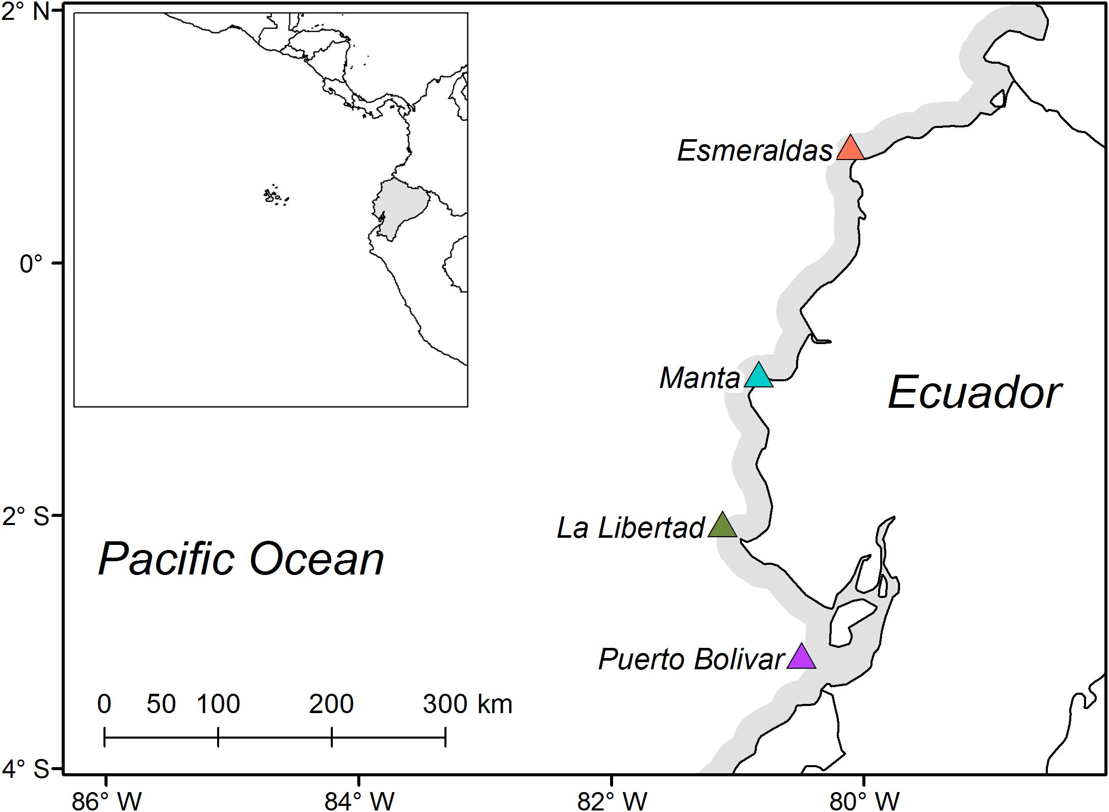
Figure 1. Sampling sites; Esmeraldas (00°55′16.0″N; 80°06′24.0″O); Manta (00°52′45.0″S; 80°50′05.2″O); La Libertad (02°03′55.0″ S; 81°07′15.0″O); Puerto Bolivar (03°06′10.0″S; 80°29′47.0″O).

At each sampling station, 200 mL water samples were collected in plastic bottles from surface, 10, 20, 30, 40, 50, and 75 m depth using a 3 Liter volume Vand Dorn bottle, then preserved in neutral Lugol’s solution (final concentration 0.4%). Samplings were performed monthly from February 2013 to December 2017, between 09h00 to 12h00 am.

Phytoplankton Identification and Abundance Estimation

Water samples were settled in 25 mL volume Utermöhl chambers (Utermöhl, 1958), and observed in a Leica (ML) inverted microscope after 24 h. Cell abundance estimation was performed in horizontal transects of the chamber at 400× magnification. Results are reported in cell. L⁻¹. The validity of names of the different taxa was checked on the World Register of Marine Species (Horton et al., 2018). Dinoflagellate species identification was based on Steidinger and Jangen (1997); Hoppenrath et al. (2009)Hoppenrath et al. (2014); Omura et al. (2012), and Lassus et al. (2016). The list of toxic species was checked on the Taxonomic Reference List of Harmful Micro Algae (Moestrup et al., 2009).

In Esmeraldas and Puerto Bolívar no sampling was performed during February to December 2016 due to economic issues.

Environmental Variables

Temperature and salinity vertical profiles were obtained using a SBE 19plus V2 SeaCAT Profiler CTD, at each sampling site. Data was processed using the SEABIRD software. Water samples for dissolved oxygen and nutrient estimation were collected with Van Dorn bottles at same depths as for phytoplankton analysis. Determination of dissolved oxygen for each sample was carried out in situ following the protocol for Dissolved Oxygen Test PEE/LAB-DOQ/01-INOCAR based on Apha (2005). Water samples for nutrient analysis were filtered with 0.45 μm millipore filters and kept at −20°C. Nitrate, silicate and total phosphate were analyzed by techniques described in Test PEE/LAB-DOQ/01-INOCAR based on Strickland and Parsons (1972). For phosphates, as values in Equatorial Pacific waters are below 3 μmol. L⁻¹, the analysis followed is detailed in Part II of the protocol cited above. In Esmeraldas and Puerto Bolívar there is no data for dissolved oxygen and nutrients from February to December 2016 due to economic issues. In this study N/P is the ratio between Nitrate and Phosphate.

Data Analysis

Before any formal statistical analysis, an exploratory data analysis (EDA) was conducted to both, environmental and biological databases in order to avoid further statistical problems (i.e., proper family distribution of the variable, homoscedasticity, independence of the values), as suggested by Zuur et al. (2010). Beside this, the environmental variables were inspected in order to avoid collinearity (i.e., correlation among explanatory variables), thus all variables who showed a Pearson correlation coefficient (rho) higher than 0.7 were dropped from the analysis (Supplementary Figure S1). Community analysis considered the calculation of the common Shannon-Weaver diversity index and its spatio-temporal variability. From an ecological perspective those species with a percentage of occurrence higher than 2% were related with the environmental variables using a canonical correspondence analysis (CCA) for each year (ter Braak and Verdonschot, 1995) through the “cca” function of the vegan package (Oksanen et al., 2018). The significance of the models were achieved through the function “anova.cca” (from the vegan package, op.cit) which performs an ANOVA like permutation test using 999 permutations (Borcard et al., 2018). All the statistical analysis were conducted under the R software (R Core Team, 2018; version 3.4.4) and supervised by OneMind-DataScience¹.

Results

Dinoflagellate Community

Dinoflagellate Occurrence

During the studied period, a total of 102 dinoflagellate taxa were identified, corresponding to 8 orders, 22 families and 31 genera (Table 1). The genera Tripos and Protoperidinium were the most diverse, comprising 22 and 16 species, respectively (Table 1).

TABLE 1

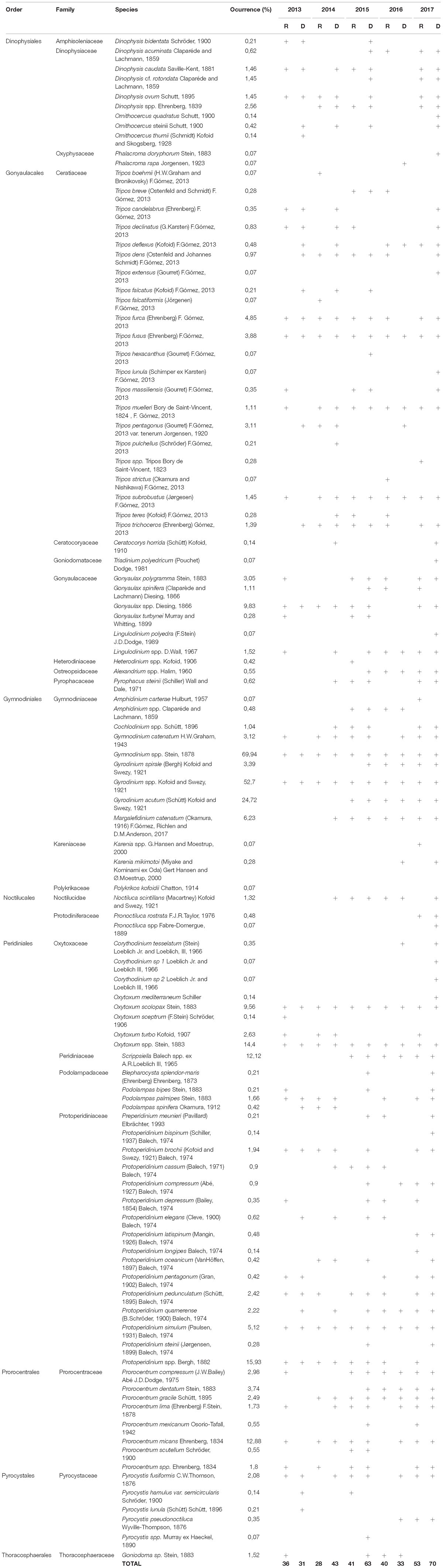
Table 1. Occurrence of dinoflagellates taxa (D, dry season; R, rainy season; + presence).

The most dominating taxa were Gymnodinium sp (70% occurrence), Gyrodinium sp (53%), and Gyrodinium acutum (21%). Other representative genera were Protoperidinium spp (16%), Oxytoxum spp (14%), Prorocentrum micans (13%), Scripsiella spp (12%), Gonyaulax spp (10%), and Oxytoxum scolopax (9.5%). The rest of the taxa presented lower percentage of occurrence (Table 1).

With respect to the temporal variability of the species mentioned above (most representative in terms of occurrence), Gymnodinium sp, Gyrodinium sp, Oxytoxum spp, and O. scolopax were present during the entire study period (Table 1). Gonyaulax spp was present also for both seasons (wet and dry seasons) and all years except 2016, which was not observed (Table 1). Gyrodinium acutum and Scripsiella spp was found in both wet and dry seasons, but only for the 2015 to 2017 period (Table 1).

Protoperidinium spp was found also in both wet and dry seasons but for the 2013–2015 period (Table 1). Instead, for the years 2016 and 2017, Protoperidinium spp was only observed during the dry season. P. micans was only found in dry season for 2013 and for wet season in 2016; instead during the period 2015–2017, P. micans was present in both seasons (Table 1).

Spatio-Temporal Variability

The two most dominant species, Gymnodinium sp and Gyrodinium sp, were more abundant in Manta, with bloom formation up to 1.2 × 10⁶ cell. L⁻¹ for Gymnodinium sp in April 2017 (Figure 2A) and 5.4 × 10⁴ cell. L⁻¹ for Gyrodinium sp in February 2016 (Figure 2B).

FIGURE 2

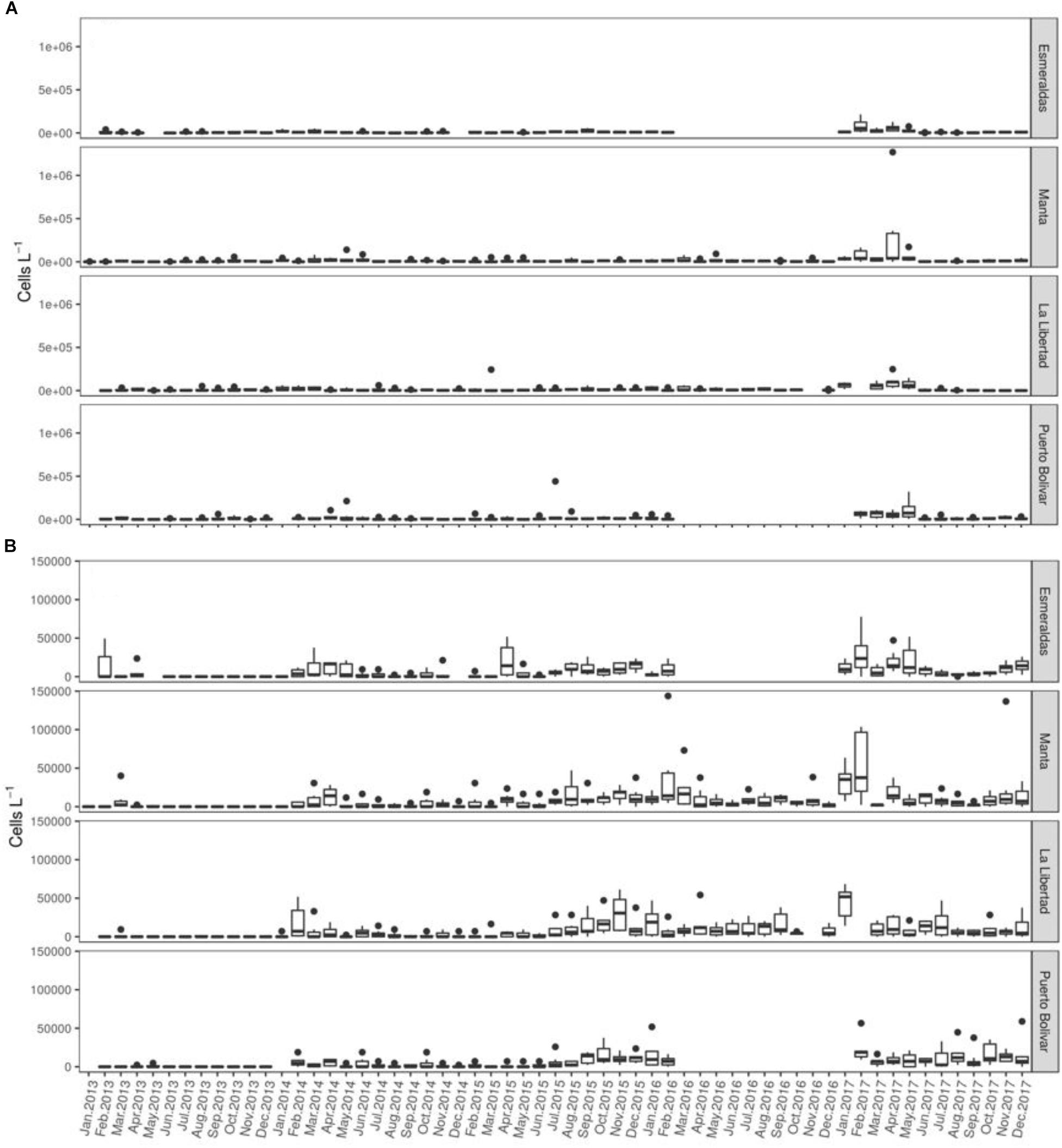
Figure 2. Dinoflagellate cell abundance estimation (cell. L⁻¹). Spatio-temporal variability of (A) Gymnodinium spp. (B) Gyrodinium spp. Abundance are expressed as cells L⁻¹.

Regarding cell abundance estimation, 2013 registered for the entire water column studied (0–75 m depth) the lowest abundances comparing with the rest of the years (Figure 3). For 2013, the maximum values were found at surface in La Libertad (mostly corresponding to March (2.8 × 10⁵ cell. L⁻¹) and at 10 m depth in Puerto Bolívar (mostly in February, 2.0 × 10⁵ cell. L⁻¹). In 2014, abundances were higher in the first 10 m of the water column except for Esmeraldas where abundances were similar in the first 30 m, being lower comparing with the other sampling sites for the same year (Figure 3). The maximum abundances in 2014, were observed at 10 m in Manta and at surface in Puerto Bolivar (with the maximum value corresponding to May, with 2.9 × 10⁵ cell. L⁻¹ and 3.8 × 10⁵ cell. L⁻¹, respectively). In 2015, Esmeraldas registered again the lowest concentrations in the first layers, comparing with the other sampling sites for the same year. The same vertical pattern was observed, as in 2014, with similar abundances from surface until 30 m (Figure 3). Maximum of the year occurred in La Libertad at surface, in March (1.1 × 10⁶ cell. L⁻¹) and at 20 m depth in Puerto Bolívar in July (maximum value of 4.5 × 10⁵ cell. L⁻¹). No peaks were registered during the year 2016, but data is not available for Esmeraldas and Puerto Bolivar. Thus, the maximum concentrations registered were observed in the first 20 m for Manta and La Libertad sites (Figure 3). The maximum abundances were found at surface and at 75 m depth for Manta (in February with 1.7 × 10⁵ cell. L⁻¹ and 1.4 × 10⁵ cell. L⁻¹, respectively) and at surface for La Libertad site (with maximum value for March with 1.0 × 10⁵ cell. L⁻¹). The highest concentrations of the sampling period were reported in 2017 (Figure 3), mostly between January and June. The maximum abundance was found in Manta, in April at surface, 1.5 × 10⁶ cell. L⁻¹ and at 10 m depth in Manta with an abundance of 4.0 × 10⁵ cell. L⁻¹. In February, at the first 10 m layer, Manta and Esmeraldas sites registered also high abundance values (∼3.5 × 10⁵ cell. L⁻¹ and ∼ 2.5 × 10⁵ cell. L⁻¹, respectively). The pattern of decreasing dinoflagellate concentration with depth, (very significant from 20 m onward) observed in the vertical abundances’ distribution for the rest of the study period, in 2017 is not so marked (Figure 3). In 2017, high abundances are observed in more deep layers (30–40 m) respecting to the other years (Figure 3) (i.e., at 30 m in May in Puerto Bolivar with 3.8 × 10⁵ cell. L⁻¹ and at 50 m in April in Manta with 3.9 × 10⁵ cell. L⁻¹).

FIGURE 3

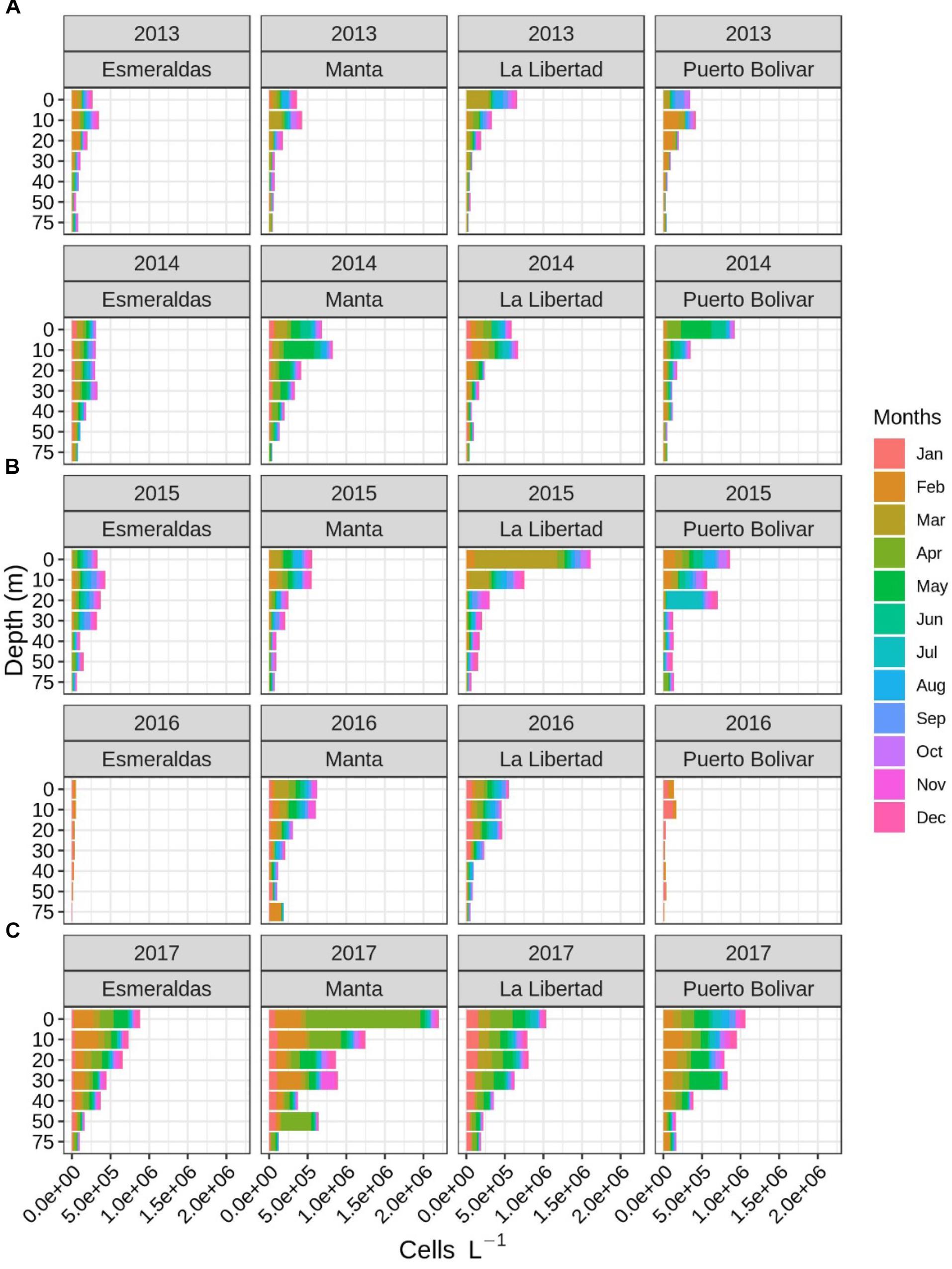
Figure 3. Spatial (horizontal and vertical) and temporal distribution of the dinoflagellate’s abundance (cell. L⁻¹) across the years (rows), sampling sites (columns), and seasonality represented by the sampling month (color bar).

Species Richness

Species richness values ranged from zero to a maximum of 21 species recorded in Puerto Bolivar during 2015 (August). Higher values were found in 0 m with a negative trend with depth (Figure 4). At surface waters (0 m) Manta and Puerto Bolívar showed the highest average values (median value of 5 for both sites), followed by Esmeraldas and La Libertad (median value of 4 for both sites). At 10 m depth the pattern is the same, except Puerto Bolívar that showed lower values (median of 4 species). Respect to the temporal variability, there is a general increase pattern along the study period, visualized as a predominance of observations above the average value across the time span of the study. In addition, along time series there are several periods were the species richness values showed the highest values. Those periods were between July to September 2013; the period between April to June 2014; February and March of 2015 in La Libertad; April and May of 2015 in Puerto Bolivar and Esmeraldas; the period of August and October in Puerto Bolivar where its maximum value was recorded; beginning of 2016, particularly for Puerto Bolivar and Manta and finally, most notably a general increase in richness values during 2017 starting in February and ending during May for the northern sites (Esmeraldas and Manta) and ending in September for southern sites (La Libertad and Puerto Bolívar). A new increase at the end of the study period (November – December) was evident for all sites. maximum richness was found in August 2015 in Puerto Bolivar at 10 and 75 m depth (20 and 21 taxa, respectively). Richness above 10 taxa were also observed the same year at same depths in La Libertad (February and March) and in 2017 at surface and 10 m in Manta (April), Puerto Bolivar (April, May, July and August) and Esmeraldas (May) (Figure 4).

FIGURE 4

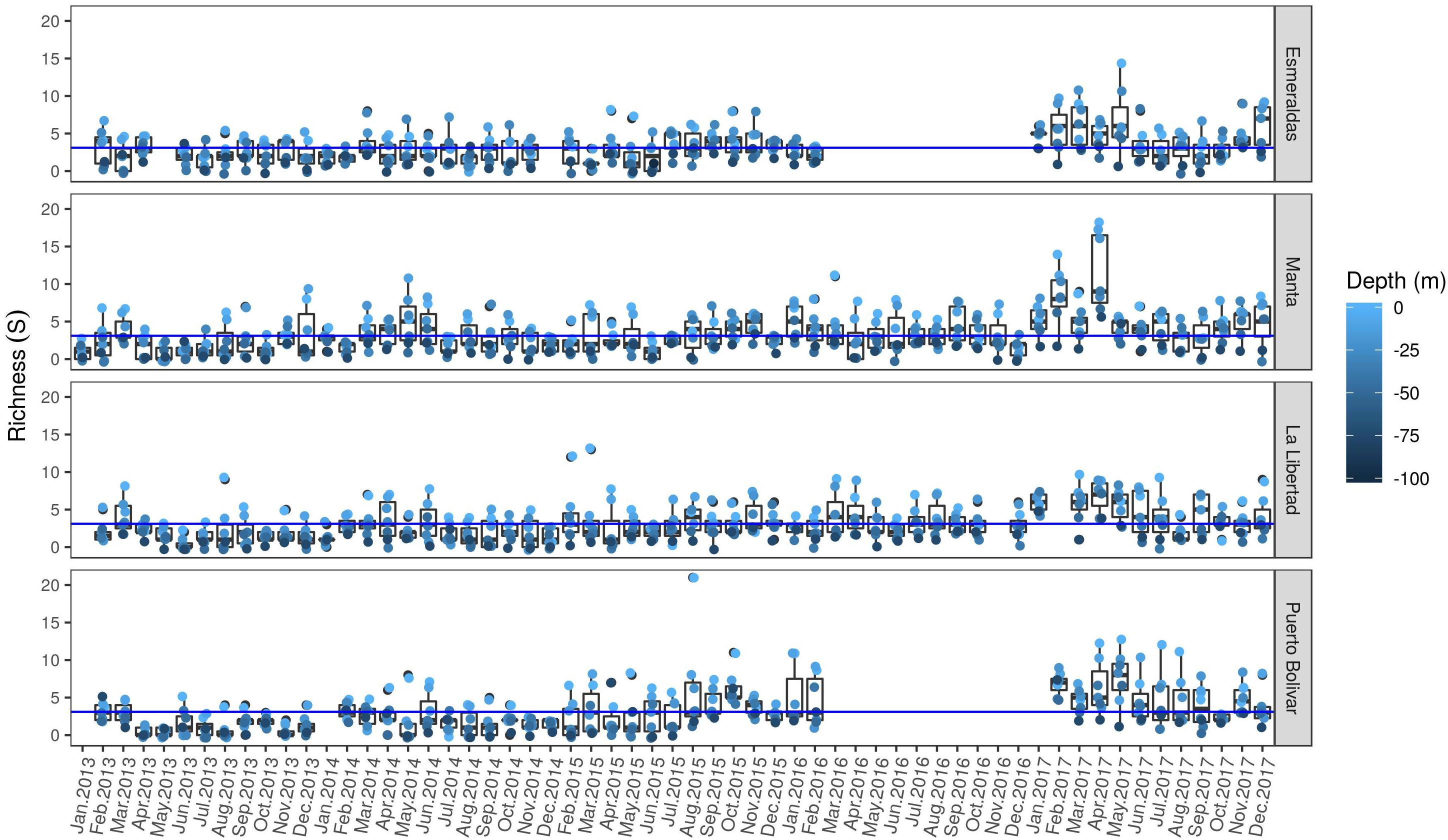
Figure 4. Spatio-temporal variability of dinoflagellates community richness. Color gradient scale represents the sampling depth. Horizontal (blue) line represents the average value for the whole study coverage.

Dinoflagellate Diversity

Diversity (Shannon–Wiener index) values ranged from 0 to 2.35 with southern stations (Puerto Bolívar and La Libertad) showing the highest values (2.21 and 2.35, respectively). In addition, higher richness values were found in surface waters across sampling stations (probably influenced by the richness gradient, see previous section) and along the sampling period. However, in some occasions high richness values were found in deeper waters during February to March 2013 (mostly for Manta and Puerto Bolivar), during the period between February to May of 2014 (except for Manta), between February to May 2015, between August to October 2015 and since the year 2017 where a general increase in diversity index was found. This general increase for 2017 showed a maximum for all sites during April – May (Supplementary Figure S2).

Harmful Algae

A total of 8 potential harmful dinoflagellate species were observed in low abundances belonging to 4 orders and 6 families, Alexandrium sp, Cochlodinium catenatum, Dinophysis acuminata, Dinophisis ovum, Gymnodinium cf. catenatum, Karenia sp., Prorocentrum lima and Prorocentrum mexicanum. The taxa that showed the highest occurrence were C. catenatum and G. cf. catenatum (6 and 3%, respectively).

The highest cell abundance was recorded by C. catenatum in May and June 2014 (7.5 × 10⁴ and 9.6 × 10⁴ cell. L⁻¹) in Puerto Bolivar. In general, the species was present in southern stations. Contrary, G. cf. catenatum was registered more times in northern stations, mainly in Esmeraldas, maximum abundances were observed in February 2013 (4 × 10⁴ cell. L⁻¹). P. lima had an occurrence of 1.5%, the highest abundance was recorded in February – March 2015 at Puerto Bolívar at surface (9.1 × 10⁴ cell. L⁻¹). Alexandrium spp, Karenia spp, P. mexicanum, D. acuminata, D. ovum, recorded the lowest occurrences (<1%) (Table 1).

Environmental Variables

Temperature and Salinity

In general, water temperature was higher in Esmeraldas compared to the rest of the stations during the studied period with a maximum in surface of 28.86°C in May 2017 (Figure 5A).

FIGURE 5

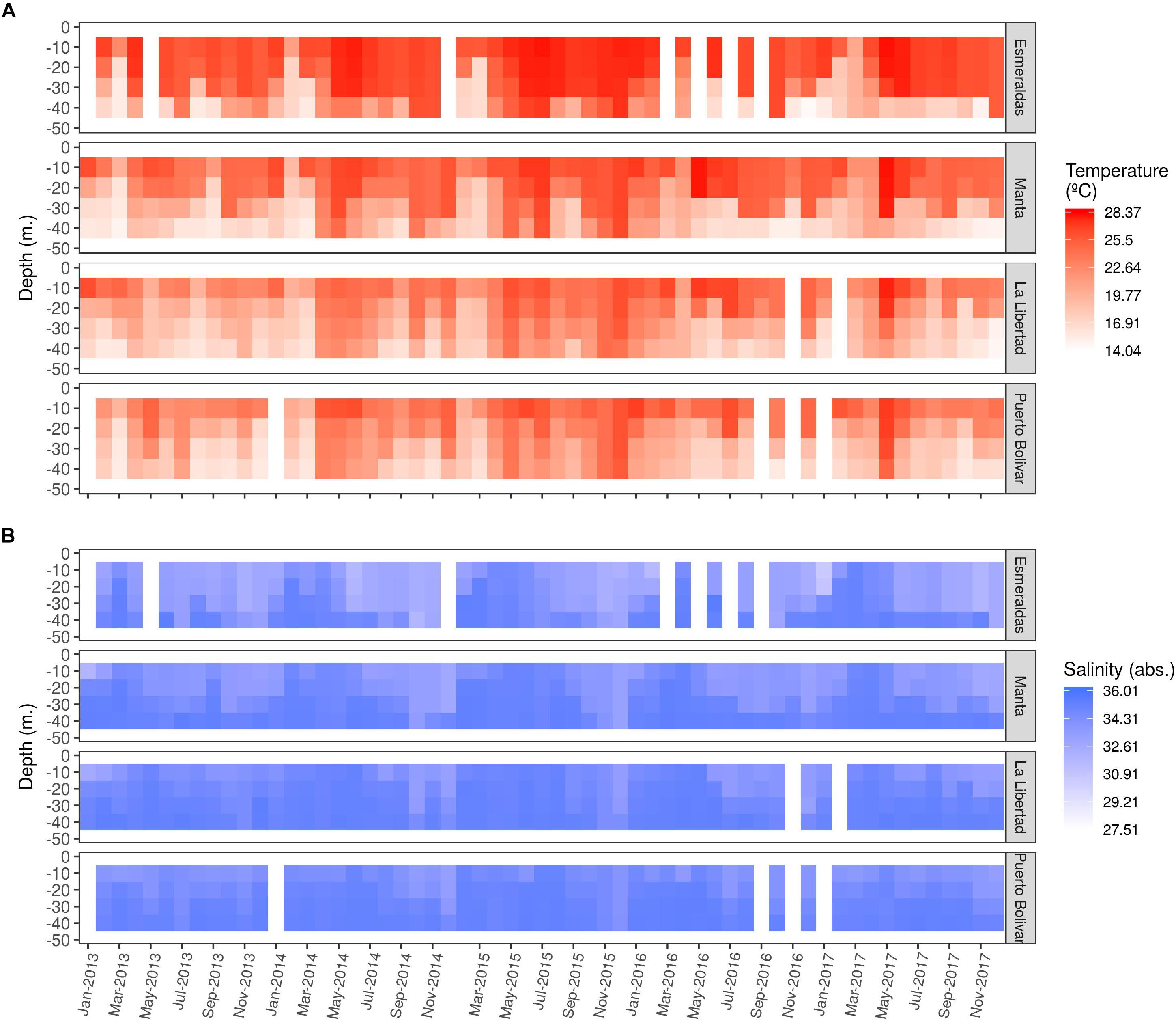
Figure 5. Spatio-temporal variability of (A) Temperature and (B) Salinity.

Concerning temporal variability, lowest temperatures (<22°C) registered in the first 10 m of the water column, occurred in 2013 from June to August in Puerto Bolivar, August and November in La Libertad, March and September in Manta and March in Esmeraldas (Figure 5A).

The next 2 years, 2014 and 2015, lowest temperatures were observed in February and March in Puerto Bolivar and La Libertad in surface and 10 m while in Esmeraldas and Manta there were also present at 20 m. In Puerto Bolivar and La Libertad the lowest values occurred in September in all depths of the water column (Figure 5A).

In 2016, lowest temperatures were reported in March in Manta for the first 20 m and in April in Puerto Bolívar from 10 m (Figure 5A).

During 2017, lowest temperatures were registered in February and March for Esmeraldas, Manta and La Libertad, while in Puerto Bolivar there were also registered in April (Figure 5A).

Contrary, higher temperatures (>25°C) registered in 2013 occurred from April to December in the first 40 m in Esmeraldas and Manta, however, in La Libertad and Puerto Bolívar, warmer waters were limited to the first layers, 20 and 10 m, respectively (Figure 5A).

In 2014 and 2015, Esmeraldas and Manta registered warmer waters in the 50 m of the water column from April to December, evident in La Libertad and Puerto Bolivar (Figure 5A).

The thermocline was deeper in northern stations, Esmeraldas and Manta (between 30 and 50 m), while in La Libertad and Puerto Bolivar it was between 10 and 30 m (Figure 5A). Annual vertical profiles of monthly mean temperature are available in Supplementary Figure S3.

Lower salinity values (<32) were observed mainly in Esmeraldas in 2013, 2014, and 2017. In the other stations, values were between 33 and 34 during the studied period in the first 30–40 m of the water column. Saltier water layers (>35.00) were present in deeper layers (between 40 and 100 m) with the exception in 2015 and 2016 where in February, April, August and October, higher salinities were observed up to 20 m (Figure 5B). Annual vertical profiles of monthly mean salinity are available in Supplementary Figure S4.

Nutrients and Dissolved Oxygen

Regarding nutrients, highest nitrate concentrations (5 a 27.6 μg-at⋅L⁻¹) were registered from 20 to 50 m, mainly during the warm season (February and March) and dry season (From July to October) in all sampling sites (Figure 6A). Lowest nitrate concentrations (<1 μg-at⋅L⁻¹) were observed in surface, up to 30 m and there was not a seasonal trend among sampling sites. In general, Esmeraldas registered lowest values compared with the rest of sampling sites. Annual vertical profiles of monthly mean nitrate are available in Supplementary Figure S5.

FIGURE 6

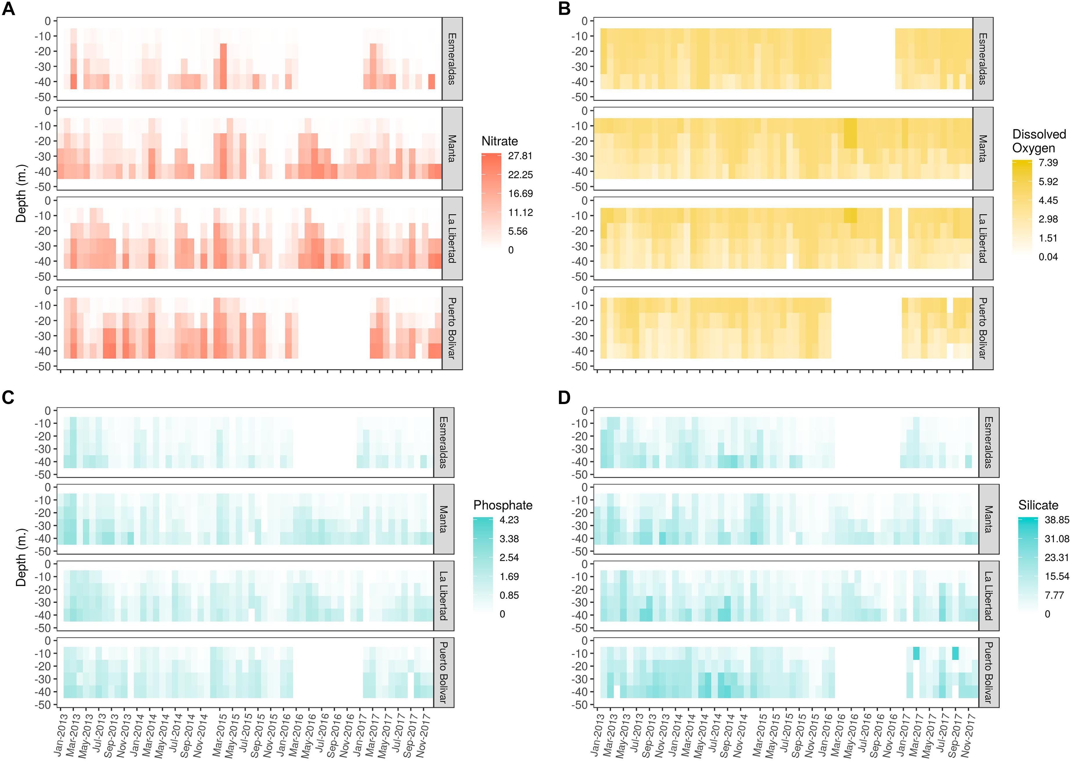
Figure 6. Spatio-temporal variability of (A) Nitrate, (B) Phosphate, (C) Dissolved oxygen, and (D) Silicate.

Concerning phosphates, highest concentrations (>1 μg-at⋅L⁻¹) were registered in 2013 in Manta and Esmeraldas in the first 50 m of the water column in February and March and between 30 and 50 m from May to September. For the rest of the years, higher values decreased between 0.3 and 1.9 ug.at/l and no seasonal pattern was observed among stations (Figure 6B).

Lowest phosphate concentrations (<0.2 μg-at⋅L⁻¹) were mainly observed in Esmeraldas without a particular pattern. Manta also registered low values but less frequency. Annual vertical profiles of monthly mean phosphate are available in Supplementary Figure S6.

Moreover, high silicate concentrations (>5 μg-at⋅L⁻¹) were registered in 2013, 2014, and 2017, with a slightly variability among sampling sites (Figure 6C). Annual vertical profiles of monthly mean silicates are available in Supplementary Figure S7.

Concerning dissolved oxygen, values in all sampling sites were between 4 and 5 mL. L⁻¹ in the first 30–40 m approximately in Esmeraldas and Manta, while in the southern sites, this layer was found in higher depth (between 20 and 30 m). More oxygenic waters (>5 mL. L⁻¹) were found occasionally in surface and 10 m layer in February and March 2013 and 2017, between April and June 2016. Lower values of dissolved oxygen (<2.5 mL⋅L⁻¹) were observed between 40 and 50 m (Figure 6D). Annual vertical profiles of monthly mean silicates are available in Supplementary Figure S8.

Relationship With Environmental Variables

For those species with a percentage of occurrence higher than 2.8% the association between the environmental variables and the structure of dinoflagellates was inspected through CCA per year. Results showed for year 2013 a significant proportion of total constrained inertia (TCI) explained by the environmental variables (TCI = 8%, p-value < 0.05) with the first two axis explaining more than 80% of this constrained inertia (Table 2). Permutation showed that salinity, phosphate and temperature significantly affected the community structure for this year (Table 3). The community composition (CCA analysis) showed that the species, Protoperidinium simulum and Prorocentrum compressum, were positively correlated with salinity and with N/P (this last being non-significant). The taxa Oxytoxum sp and Protoperidinium sp. were positively associated with high values of nitrite. The group formed by Gymnodinium cf. catenatum, Oxytoxum turbo and P. micans were positively associated with high values of temperature and negatively with salinity and N/P values. N/P is the ratio between nitrate and phosphate in this study, low N/P ratio have been associated to HAB occurrence. In relation with salinity the species O. scolopax, Gyrodinium sp and Gonyaulax polygramma showed a negative association with this variable. Finally, the group formed by the species Gonyaulax sp, Gymnodinium sp, Tripos fusus and Tripos furca were negatively associated with nitrite and phosphate, but showed an unimodal response with the rest of the variables (a central position in the CCA-Triplot, Figure 7A).

FIGURE 7

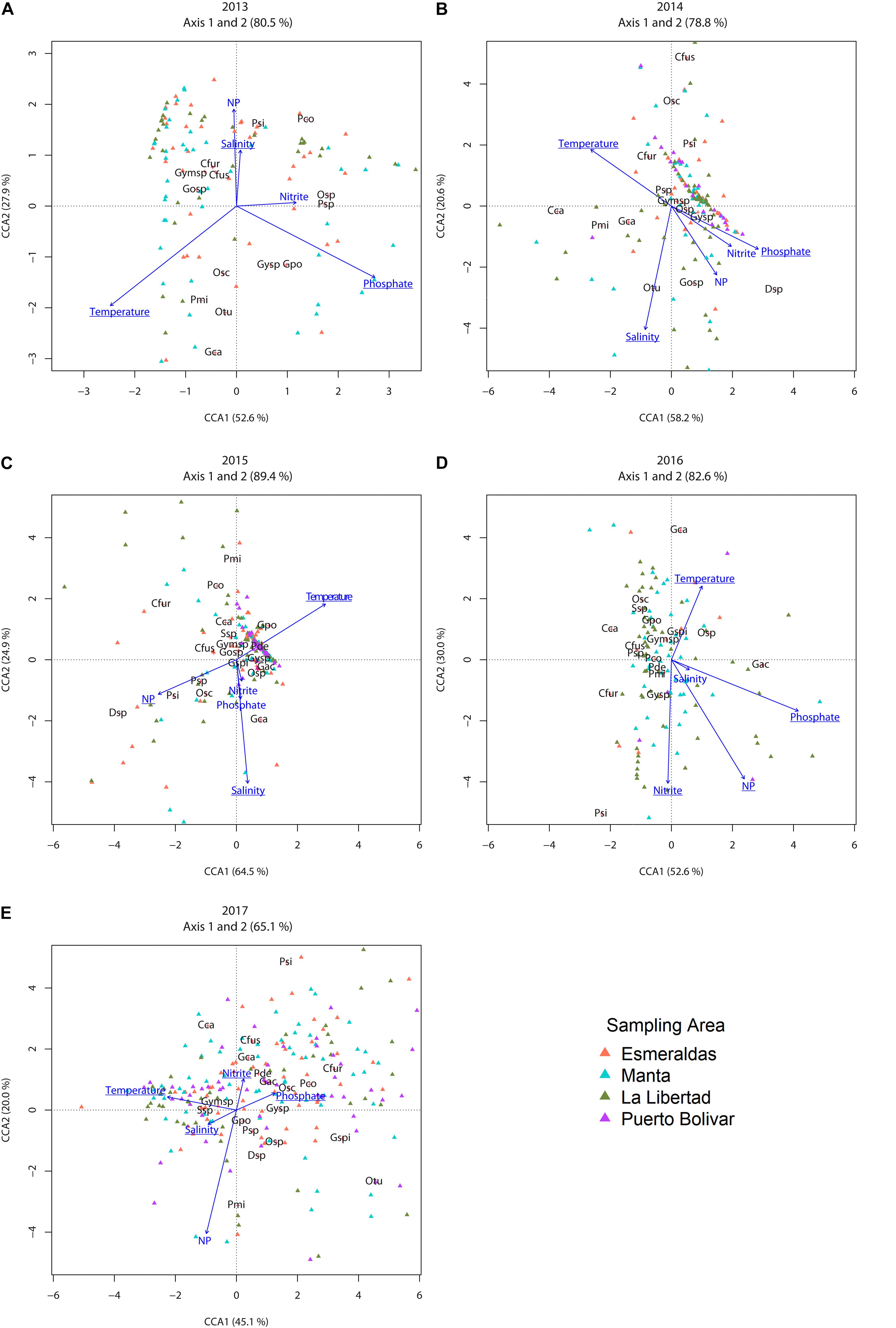
Figure 7. Canonical correspondence analysis triplot for (A) 2013, (B) 2014, (C) 2015, (D) 2016, and (E) 2017. Sampling stations are shown as triangles with color-code according to the sampling area (figure legend). The species (with occurrence >2%) present in the community CCA analysis follows: Otu, Oxytoxum turbo; Pco, Prorocentrum compressum; Gpo, Gonyaulax polygramma; Gca, Gymnodinium cf. catenatum; Gspi, Gyrodinium spirale; Pde, Prorocentrum dentatum; Cfus, Tripos fusus; Cfur, Tripos furca; Psi, Protoperidinium simulum; Cca, Cochlodinium catenatum; Osc, Oxytoxum scolopax; Gosp, Gonyaulax sp; Ssp, Scripsiella sp; Pmi, Prorocentrum micans; Osp, Oxytoxum sp; Psp, Protoperidinium sp; Gac, Gyrodinium acutum; Gysp, Gyrodinium sp; Gymsp, Gymnodinium sp. Environmental (explanatory) variables are indicated in blue [“Temperature anomaly” (abbreviated in the figure as “Temperature,” °C), “Absolute salinity anomaly” (abbreviated in the figure as “Salinity,” “Nitrite,” “Phosphate,” and the ratio nitrate – phosphate (abbreviated in the figure as “N/P”); bold underline correspond to significant explanatory variables according to permutation test (see methods)]. The percentage of variability (inertia) explained is indicated on each axis.

TABLE 2

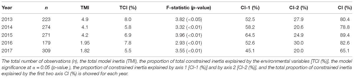
Table 2. Summary table of canonical correspondence analysis (CCA) statistics per year.

TABLE 3

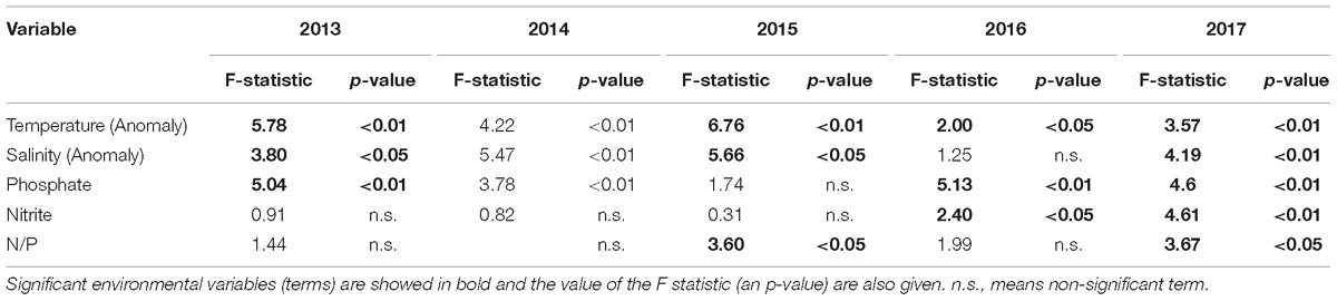
Table 3. Summary table of the permutation tests over the CCA results.

For year 2014 a lower than previous year, but still significant proportion of TCI explained by the environmental variables (TCI = 5.8%, p-value < 0.05) with the first two axis explaining 78.8% of this constrained inertia (Table 2). For this year (same as 2013) salinity, temperature and phosphate significantly affected the community structure (Table 3). Moreover, a clear positive correlation between phosphate with nitrite and N/P (both being non-significant) and those three variables showed a negatively association with temperature (Figure 7B). The association of species with environmental variables showed that Dinophysis sp was positively associated with N/P and nitrite – phosphate variables. With respect to salinity Oxytoxum turbo was positively associated whereas T. fusus, O. scolopax and P. simulum were negatively associated. T. furca and C. catenatum (in a lesser extent) showed a positive association with temperature. The rest of the species showed a central position in the CCA-Triplot representing unimodal response to the environmental variables (Figure 7B).

For year 2015 the proportion of TCI explained by the environmental variables was also significant (TCI = 5.8%, p-value < 0.05) with the first two axis explaining the highest amount of this constrained inertia along the study period (89.4%, Table 2). During 2015 the temperature, the N/P ratio and salinity were those variables which significantly explained the dinoflagellate’s community structure (Table 3). A positive relationship was observed among salinity and nitrite and phosphate and a negative association between temperature and N/P (Figure 7C). From the species-specific relationship, the CCA analysis revealed a positive association between Dinophysis sp and P. simulum with N/P ratio and negatively with temperature. The species Gymnodinium cf. catenatum was associated with positive values of nitrite and phosphate and in a lesser extent, showing a non-linear response, with salinity. Finally, the species P. micans, P. compressum and T. furca were associated to low values of salinity (negative relationship) (Figure 7C). Interestingly, this year none species was associated with high, but low temperature values.

For year 2016 and 2017 a decrease in the TCI from 7.8% to 5.5 was evident. However, for both years the model was able to significantly explain this constrained inertia with the first two axes explaining 82.6% and 65.1% of this constrained inertia, respectively (Table 2). Particularly during 2016 the environmental variables who were significantly associated with the structure of the dinoflagellate community were temperature, nitrite and phosphate (Table 3). Salinity and phosphate were positively correlated and temperature and nitrite were negatively correlated. The CCA analysis for this year showed that Gymnodinium cf. catenatum was correlated positively with salinity and negatively with nitrite. The species Gyrodinium acutum was associated with high values of phosphate with a non-lineal response (center position of the species related with the environmental vector). The species C. catenatum, O. scolopax, Scripsiella sp, G. polygramma, T. furca, Protoperidinium sp and Gymnodinium sp. showed a negative association with phosphate and Oxytoxum sp, Gyrodinium spirale, G. polygramma, Scripsiella sp, O. scolopax, and Gymnodinium sp a negatively association with nitrite (Figure 7D). During 2017 all the environmental variables were significant when related to the observed dinoflagellate community structure (Table 3). Among the environmental variables, a negative association was evident for salinity and phosphate (Figure 7E). From the community composition perspective, the species P. simulum, T. fusus, Gymnodinium cf. catenatum, and Prorocentrum dentatum showed a clear positive relationship with nitrite and negatively with salinity and with the N/P ratio. The species T. fusus, P. compressum, O. scolopax, and Gyrodinium sp were positively associated with phosphate and negatively with salinity. For this year, non-species were related positively with temperature, but some species showed a negative association with this environmental variable (e.g., Oxytoxum turbo, Gyrodinium spirale, Oxytoxum sp, and Gyrodinium sp).

Interestingly, the total model inertia (TMI), which represents the total variability n-dimensional inside the model, remained more or less constant for the first 3 years (2013–2015) ranging from 4.1 to 4.9. However, during years 2016 and 2017 this TMI was significant lower with values for 2016 of 1.95 and for 2017 a TMI of 1.82 (Table 2).

Discussion

Dinoflagellate Community

In this study, there were reported a total of 97 taxa, corresponding to 8 orders, 22 families, and 31 genera during the sampling period from 2013 to 2017 in 4 stations in the coast of Ecuador at different depths. Phytoplankton dynamics across the ETP coast is more characterized in other countries and there is a lack of information in the central area corresponding to the Ecuadorian coast. Interestingly, recent studies regarding phytoplankton distribution in response to ENSO events have been published (Conde and Prado, 2018; Conde et al., 2018), but, unfortunately, species identification is not indicated as a result. Another recent study explored the oceanography of red tides using remote sensing data from 1997 to 2017, confirmed that potential HABs have been dominated by dinoflagellates during wet season mostly at the Gulf of Guayaquil (Borbor-Cordova et al., 2019). Furthermore, dinoflagellates abundance reported in the present study was not high and the number of proliferations was low, only Gymnodinium sp exceeded 10⁶ cell. L⁻¹ in April 2017. In the coast of Ecuador, INOCAR and other researchers have reported blooms of dinoflagellates, for example Gymnodinium sp was reported in 2003, 2004, 2005 reaching high concentrations (1 × 10⁵ cell. L⁻¹ – 1.1 × 10⁷ cell. L⁻¹) in the Gulf of Guayaquil both in wet and dry season (Torres and Tapia, 2002; Torres et al., 2017).

It is important to mention that species identification resulted difficult to perform without specific equipment and adequate formation. In that sense, some of the taxa found in the area were not identified at species level. Dinoflagellates identification under inverted microscope based on morphological features constitutes a challenge since some species from several genera share the same plate pattern and overlap in size (e.g., the genus Ostreopsis – Carnicer et al., 2016). In the last decades, molecular techniques have allowed to perform accurate identifications in dinoflagellates using rDNA sequences (Litaker et al., 2007). Unfortunately, there is no molecular characterization of marine dinoflagellates in the Ecuadorian coasts, with the exception of Ostreopsis cf. ovata (Carnicer et al., 2016). It is important for Ecuadorian institutions to invest in the implementation of molecular techniques for future investigations, especially important to identify potentially toxic species.

Higher species richness in the water column was observed in surface layers, with a maximum of 21 taxa. These results are in agreement with a study performed in 2015 at the southern coast of the country, in El Oro province, where they reported species richness average between 28 and 23 dinoflagellates in surface samples (Prado et al., 2015; Conde et al., 2018). The time series length of the present study avoids us to conduct a formal time series analysis to statistically prove this increase pattern observed. In addition, some oscillatory behavior is evident and probably associated with the interannual variability pattern (Conde et al., 2018).

In 2015, associated with El Niño ENSO event, higher dinoflagellate species richness values were registered during the wet season in La Libertad, Puerto Bolivar and Esmeraldas, reaching a maximum of 28 species in dry season in Puerto Bolivar, that could be linked with upwelling and higher nutrients concentrations (Borbor-Cordova et al., 2019). In 2017, higher values are also observed in each station with the highest found in Puerto Bolivar in agreement with Prado et al. (2015), associating the event with the presence of the Humboldt current. The higher amount of species during El Niño ENSO events can be linked with the transport of species from the advected waters due to the current, as well as upwellings occurring in the equatorial region (Pennington et al., 2006; Gierach et al., 2012).

Regarding potential harmful dinoflagellates, a total of 8 taxa were observed, Alexandrium sp, Cochlodinium sp., D. acuminata, D. ovum, Gymnodinium cf. catenatum, Karenia sp., P. lima and P. mexicanum but not HABs were observed. In Torres (2015), a total of 131 HABs were registered from 1968 to 2009 in the same sampling sites as the present study, where toxic dinoflagellate community was similar to the species listed above. Unfortunately, no statistics analysis was performed in Torres (2015), however, they concluded that during wet-warm season the highest number of HABs events occurred, being more abundant in the Gulf of Guayaquil, southern station. Due to the low abundances registered in the present study, CCA analysis was not possible to perform with toxic species, which do not allow to confirm this hypothesis. Furthermore, an historical reconstruction of blooms from 1997 to 2017 in the Ecuadorian coast, highlighted the presence of toxic species such as Gymnodinium cf. catenatum, P. micans, C. catenatum and Dinophysis caudata among others. As for the present study, lower abundances were registered for toxic species, slightly higher in the Gulf of Guayaquil than in La Libertad and Manta (Borbor-Cordova et al., 2019). Unfortunately, Esmeraldas was not considered in the study and data corresponded only to wet season.

During these studies performed by the INOCAR, no toxic analysis has been performed in water samples due to a lack of specialized laboratory. This fact highlights the necessity of specific equipment acquisition by the government in order to control the presence of toxins in the productive areas, not only limited to monitoring phytoplankton abundances.

Environmental Variables and Seasonality

Overall, in this study, SST and salinity anomalies, nutrients, as well as the N/P ratio were strongly associated to the spatio-temporal distribution of dinoflagellate community (Figure 7). Studies elsewhere have found that HAB have been related during positive anomalies of SST, stratification with a deeper thermocline, pulses of upwelling during summer or dry season and the biological interaction among phytoplankton community (Hallegraeff, 2010; Díaz et al., 2016), some of these conditions were found in this analysis.

The environmental variables presented in this study confirm the main patterns of current systems on the ETP, which are driven by cold Humboldt Current in the central and south coast of Ecuador (La Libertad and Puerto Bolivar), associated with the equatorial upwelling (EU) system and the warm Panama current toward the north of Ecuador (Esmeraldas), these oceanographic settings drives the biogeochemical conditions that may promote extensive phytoplankton growth and potential HABs (Cucalon, 1989; Pennington et al., 2006). The north of the Ecuadorian coast is under the influence of the inter-tropical convergence zone (ITCZ), receiving higher levels of precipitation as well as runoff from Panama Gulf generating a low salinity and warmer temperatures which lead to stratified conditions, shallow halocline-nutricline (30–40 m), and low nutrients concentration (Pennington et al., 2006). Those conditions are reflected in the northern station of Esmeraldas, where minimum dinoflagellate abundances were reported (Figure 2 and Supplementary Figure S2) compared to other stations, highlighting the influence of the oceanographic characteristics and strong seasonality of the ETP (Chavez et al., 2002).

Oceanographic studies have established the seasonal pattern of the coastal EU at the center of Ecuador, and the upwelling from the Humboldt Current on the south of the Ecuadorian Coast (Pennington et al., 2006). Seasonality of those upwelling system are reflected in all stations (based on higher nutrient concentrations and lower temperatures) except at Esmeraldas, being deeper and high nutrient concentration during wet season (December to May) but also between August to September. It is expected that Manta is mostly influenced by the EU while at La Libertad and Puerto Bolivar it is the upwelling of Humboldt Current, considered one of the most productive of the world (Chavez et al., 2002; Pennington et al., 2006; Oyarzún and Brierley, 2018). In this study, highest concentrations of dinoflagellates were found in Manta (April 2017), La Libertad (March 2015), and Puerto Bolivar (May 2014 and May 2017), during wet season. During this period, there is a large amount of nutrients coming with the intense runoff from the agricultural Guayas Basin (Borbor-Cordova et al., 2006) and interestingly, in the present study it is reported higher levels of nutrients, mainly nitrate and phosphate (Supplementary Figures S5, S6), coming from deeper water, suggesting advection from the coastal Humboldt Upwelling in dry season with peaks on August. Thus, data on this study suggests that a combination of extreme hydrodynamic conditions, climate variability associated to the warm phase of the Pacific Decadal Oscillation (PDO) and ENSO in the coast of Ecuador (2015–2016), influencing salinity and SST anomalies and nutrient limitation conditions, led to shifts in the phytoplankton community and maybe to HABs.

In this region phytoplankton productivity and growth are influenced by the upwelling dynamics which can be associated to the pycnoline-nutricline-oxycline depth, and their variability along the coast is driven by local specific conditions of coastal waves, seasonality and inter-annual variability of ENSO cycle (Montecino and Lange, 2009). The thermo-nutricline determines the supply of limiting nutrients (related to N/P ratio) to the euphotic zone and influencing the phytoplankton community assemblage during each ENSO event. This is evidenced in the present study with the inter-annual variability of dinoflagellates associated to ENSO events which is characterized by high positive anomaly of SST, changes on the timing of seasonality and strengthening (cold phase) or weakening (warm phase) the coastal upwelling (Pizarro and Montecinos, 2004; Pennington et al., 2006; Montecino and Lange, 2009). Similar dynamics have been reported in North and ETP during ENSO events (Chavez et al., 2002; Jacox et al., 2016). Previous ENSO studies pointed out that southwest winds weakness lead to a coastal upwelling decline which diminish phytoplankton blooms occurrence (Tam et al., 2008; Wang et al., 2008; Montecino and Lange, 2009). However, during warm phase ENSO event in 2015 occurred anomalous conditions related with sustained wind stress, intermittent coastal upwelling, that could be the reason why dinoflagellates were able to persist even in a nutrient limited environment, and warm stratified conditions (Smayda and Reynolds, 2001; Du et al., 2015; McCabe et al., 2016; McKibben et al., 2017; Conde and Prado, 2018).

During the period of this study (2013–2017), 2013 is considered a normal year with the lower abundances of dinoflagellates of the study, a weak ENSO warm phase in 2014, followed by a strong warm phase ENSO in 2015–2016 (with a different seasonality of the one in 1997–1998) beginning a transition to cold phase ENSO during the dry season 2016 is extended to 2017 characterized by abundance of dinoflagellates (see Figure 3). Each year of the study develop specific environmental conditions; however, SST anomalies, salinity and nutrients persistently drove the dinoflagellates community for all the study period (see Figure7).

In 2013 a normal year with a slightly cold SST anomaly (see Supplementary Figure S9), lower salinities, and nutrients were the drivers for the dinoflagellates. Gymnodinium cf catenatum, Oxytoxum turbo and P. micans were associated to less saline, low nutrients and warm waters typical conditions during wet season in Esmeraldas influenced by the Panama Current. While P. simulum, P. compressum, Oxytoxum sp, and Protoperidinium sp are positively related to nutrient and salinity which are characteristics of upwelled waters, suggesting a preference of nutrient-rich water along the coast of Ecuador (Figure 7A).

In 2014, considered a weak ENSO year with ONI strong anomalies (>1.5) during wet season decreasing rapidly toward December 2014 (see Supplementary Figure S9). T. fusus, O. scolopax and P. simulum were associated to low salinity conditions mostly on Esmeraldas, Manta and La Libertad suggesting iN/Put of freshwater runoff and precipitation. While Dinophysis sp was associated to nutrients from upwelled waters from EU system at the Esmeraldas station, the upwelling process is related with the nitrate distribution at 30–50 m (Supplementary Figure S5). T. furca and C. catenatum were associated to positive anomalies of temperature, suggesting that have adapted to the warm conditions on the Esmeraldas site.

Although the SST anomalies of ENSO events in 2015 were of similar magnitude to those in 1997–1998, the responses were diverse in relation to the oceanographic characteristic of the equatorial front (Conde et al., 2018). By April 2015, the thermocline deepened to 40–75 m until December 2015 generating stable thermal stratification, but nutrients were sustained by a weak upwelling and a pycnocline-nutricline between 30–50 m. Even though the nutrients were reduced at the surface layer (see Figures 6, 7), surprisingly the abundance levels of dinoflagellates in La Libertad and Puerto Bolivar where high between 10–30 m (see Figure 3). By August 2015, nutrients (nitrate, and phosphate) were upwelled between 30 and 50 m at La Libertad, and Puerto Bolivar. These conditions of thermal stratification, deepened thermocline, slightly upwelling, light for growth and ciliate prey (Mesodinium rubrum) appear to establish the optimal combination for the development of potential HABs such as Dinophysis sp and P. simulum (Reguera et al., 2012; Díaz et al., 2013). G. catenatum have affinity for the nitrate and phosphate and less with salinity, bloom of this specie has been related to advected vegetative populations to the coasts during the relaxation of coastal upwelling (Bravo and Figueroa, 2014). P. micans, P. compressum, and T. furca were associated to less saline water characteristic of the Panama current or influenced by precipitation at the northern stations of Esmeraldas and Manta. Considered an extreme ENSO year and warm PDO, expecting a limited algal growth, surprisingly there was a relative high abundance of dinoflagellate and higher richness reflexed in the diversity of species (21). If this increase in richness is a pattern of the ENSO need to be verified in other years.

Year 2016 shows the transition between a warm ENSO to cold and normal conditions, with ONI decreasing from 2.5 in January to – 0.7 in September in the dry season (see Supplementary Figure S9). In this year, Gymnodinium cf. catenatum appeared during dry season associated with salinity and inversely with nitrite at the Manta and La Libertad, unfortunately no data in Esmeraldas and Puerto Bolivar are available. Gymnodinium cf. catenatum has been recognized to cause paralytic shellfish poisoning across regions and as a survivor by using strategies based on its motile forms and cysts in plankton assemblages and in surface sediments (Yamamoto et al., 2004; Bravo and Figueroa, 2014). Gymnodinium cf. catenatum is also identified as one of ten most damaging potential domestic target species, considering the environmental and economic impact in aquaculture and also in human health (Hallegraeff, 2003). C. catenatum is another specie that seems to be associated to the upwelling at La Libertad in dry season.

During 2017, persistent negative SST anomalies associated to upwelling and water nutrients richness lead to an increase in the productivity of the region in all the ETP (Brown et al., 2015). Concentrations of dinoflagellates increased and reached their maximum in all the stations due to conditions of a persistent upwelling specially in Puerto Bolivar station. Some of the species that were associated with upwelled nutrients were P. simulum, T. furca, Gymnodinium cf. catenatum and P. dentatum.

In the present study, the most abundant species were Gymnodinium sp and Gyrodinium sp which were present every year in both seasons of the studied period and registered up to 40 m depth. Those species correspond to free living large cell dinoflagellates, ubiquitous in the Pacific Ocean, previously registered in México, California and Ecuador (Gomez, 2005; Meave-del Castillo et al., 2012; Torres, 2015). Both species appeared in all coastal stations during the seasonal transition in the weak ENSO in 2014 and strong ENSO in 2015 (Figure 2 and Table 1) indicating their capacity to adjust to warm and deeper thermo-nutricline.

Even though some microalgae exhibit a rapid adaptability to high temperatures in short-term experiments, the physiological plasticity and genetic response of many microalgae under future environmental conditions is unknown (Hallegraeff, 2010). Organism size and elemental composition of the phytoplankton community will influence processes at the level of individuals, populations, communities and ecosystems (Finkel et al., 2010). Some researchers have found that dinoflagellates are species with a smaller surface and have the ability to grow and sustain during ENSO, ocean heatwaves, stratified conditions, and nutrient poorer waters (Smayda and Reynolds, 2003; Glibert et al., 2005). However, there is also evidence that nutrient enriched waters can stimulate dinoflagellates blooms (Glibert et al., 2005), therefore, dinoflagellates are considered strategist and survivors either in extreme conditions.

The contrasting behavior of Tripos species in divergent lake types (with different climatic, morphometric, geological, hydrological, and trophic features) explains the existence of ecotypes of these species adapted to diverse environmental conditions and exhibiting high intra- and inter-population and morphological variability (Cavalcante et al., 2016). T. furca is also known to perform active vertical migration, depending on nutrients and water temperature in both natural and laboratory conditions, which means that different species of dinoflagellates have different ecological abilities. These abilities are possibly linked with their ecological responses for surviving under local environmental conditions. T. furca has a competitive advantage because of physiological adaptations to low nutrient concentration waters (Baek et al., 2011). Therefore, dinoflagellates can alter their vertical position in the water column by swimming, which allows them to maintain an optimal depth in terms of light or nutrients. Consequently, the actual duration of high irradiance in the coastal bays is considered to regulate the maintenance of the bloom (Baek et al., 2011).

In general, under N or P limitation or some specific N/P ratio, some toxic dinoflagellates are probably outcompeted, and toxin production may be an adaption strategy to offset the ecological disadvantages of dinoflagellates with low nutrient affinity (Smayda, 1997). How these biochemical shifts shape phytoplankton community structure and the presence of potentially toxic species need to be explored in Ecuador.

Montecino and Lange (2009) proposed that during warm ENSO as 2015, there is microbial trophic web path mostly dominated by small-sized phytoplankton, in this study taxa such as Gonyaulax polygrama, P. dentatum and Gynmodinum spp. were characterized to be trophic web dominated. Still it is not very clear which are the main ecological drivers to explain interannual variability of phytoplankton community structure, including toxin producer species. In addition, mixotrophy relationships need to be explored because many of the motile bloom formers are mixotrophic protists (Stoecker et al., 2017). Some argued that PDO is a good indicator to explain those shifts on the community structure and potential toxins generation (Du et al., 2015). Unfortunately, in this study only dinoflagellates community was considered, so it is not possible to confirm this ascertain. An effort in future works need to be done in order to encompass more taxa to better understand phytoplankton distribution in the area.

Conclusion

Dinoflagellates abundances reported in the present study were not elevated, and no HABs were observed in the studied period. The taxa presented in this study represents a base-line in which future work may referred in order to understand certain dinoflagellate dynamics. In synthesis, the environmental variables and the oceanographic ENSO index served to understand how the current system of the ETP, their thermocline dynamics, and the coastal upwelling affect euphotic zone nutrient supply and hence, dinoflagellates abundance and richness along the coast of Ecuador.

Moreover, toxic species were detected and, considering that in future decades it is predicted an increase in seawater temperature and extreme events frequency (IPCC, 2014), phytoplankton dynamics may be influenced. In order to be able to predict future scenarios of HABs, it is important to study their distribution in relation to environmental variables in areas where extreme events may affect their proliferations. Thus, it is crucial to involve policy-makers and stakeholders in the implementation of environmental policies and climate change adaptation strategies involving long-term monitoring and sanitary programs, not covered at present.

Author Contributions

GT, SR, RN, and EP made substantial contributions to conception and design of the work and conducted the sampling, nutrient, and dinoflagellates analysis. OC, GT, MB-C, PDLF, and AC made substantial contributions in data analysis and interpretation and participated in drafting the article. MB-C gave the final approval of the version to be submitted.

Funding

This research has been developed as an international and inter-institutional collaboration among different research institutes and universities. We would like to acknowledge the following projects and institutional support: Project “Oceanic Early Warning System,” funded by National Secretary of Science and Technology (SENESCYT) and INOCAR, Project T2-DI-2014 “Climate Variability and Harmful Algae Bloom Interaction and their impact on human health on the coast of Ecuador,” funded by the Escuela Superior Politecnica del Litoral (ESPOL).

Conflict of Interest Statement

The authors declare that the research was conducted in the absence of any commercial or financial relationships that could be construed as a potential conflict of interest.

Supplementary Material

The Supplementary Material for this article can be found online at: https://www.frontiersin.org/articles/10.3389/fmars.2019.00145/full#supplementary-material

FIGURE S1 | Collinearity analysis of the environmental variables measured in the study. The Pearson’s correlation coefficients for each pair of variables are shown in the upper-right panel with the size of the text proportional to its value. Significance code represents: ^∗∗∗p-value < 0.001. Additionally, the density histogram of each variable is represented in the diagonal and a scatter plot with a smoothing spline (in red) is shown in the left-lower panel.

FIGURE S2 | Spatio-temporal variability of dinoflagellates community Shannon-Wiener (H) index. Color gradient scale represents the sampling depth. Horizontal (blue) line represents the average value for the whole study coverage.

FIGURE S3 | Annual vertical profiles of monthly mean temperature (°C) for (A) Esmeraldas, (B) Manta, (C) Libertad, and (D) Puerto Bolívar.

FIGURE S4 | Annual vertical profiles of monthly mean salinity for (A) Esmeraldas, (B) Manta, (C) Libertad, and (D) Puerto Bolívar.

FIGURE S5 | Annual vertical profiles of monthly mean nitrate for (A) Esmeraldas, (B) Manta, (C) Libertad, and (D) Puerto Bolívar.

FIGURE S6 | Annual vertical profiles of monthly mean phosphate for (A) Esmeraldas, (B) Manta, (C) Libertad, and (D) Puerto Bolívar.

FIGURE S7 | Annual vertical profiles of monthly mean silicate for (A) Esmeraldas, (B) Manta, (C) Libertad, and (D) Puerto Bolívar.

FIGURE S8 | Annual vertical profiles of monthly mean dissolved oxygen for (A) Esmeraldas, (B) Manta, (C) Libertad, and (D) Puerto Bolívar.

FIGURE S9 | Temporal series of ENSO index (A) ONI (1+2), (B) ONI 3.4, and (C) MEI index.

Footnotes

1. ^ https://onemind-datascience.com/

References

Abate, R., Gao, Y., Chen, C., Liang, J., Mu, W., Kifile, D., et al. (2017). Decadal variations in diatoms and dinoflagellates on the inner shelf of the east china sea. Chin. J. Ocean. Limnol. 35, 1374–1386. doi: 10.1007/s00343-017-6029-1

CrossRef Full Text | Google Scholar

Apha. (2005). Standard Methods for the examination of Water and Wasterwater, 21 Edn. Washington, D.C: American Public Health Association.

Google Scholar

Baek, S. H., Shin, H. H., Choi, H.-W., Shimode, S., Hwang, O. M., Shin, K., et al. (2011). Ecological behavior of the dinoflagellate Ceratium furca in jangmok harbor of jinhae Bay. Korea. J. Plankton Res. 33, 1842–1846. doi: 10.1093/plankt/fbr075

CrossRef Full Text | Google Scholar

Borbor-Cordova, M., Boyer, E. W., McDowell, W. H., and Hall, A. S. (2006). Nitrogen and phosphorus budgets for a tropical agricultural watershed: guayas. ecuador. Biogeochemistry 79, 135–161. doi: 10.1007/s10533-006-9009-7

CrossRef Full Text | Google Scholar

Borbor-Cordova, M., Torres, G., Mantilla-Saltos, G., Casierra-Tomala, A., Bermudez, R., Renteria, W., et al. (2019). Oceanography of harmful algal blooms on the ecuadorian coast (1997-2017): integrating remote sensing and biological data. Front. Mar. Sci. 6:13. doi: 10.3389/fmars.2019.00013

CrossRef Full Text | Google Scholar

Borcard, D., Gillet, F., and Legendre, P. (2018). Numerical Ecology with R, 2nd Edn. New York, NY: Springer International Publishing. doi: 10.1007/978-3-319-71404-2

CrossRef Full Text | Google Scholar

Bravo, I., and Figueroa, R. I. (2014). Towards an ecological understanding of dinoflagellate cyst functions. Microorganisms 2, 11–32. doi: 10.3390/microorganisms2010011

PubMed Abstract | CrossRef Full Text | Google Scholar

Brown, J. N., Langlais, C., and Gupta, A. S. (2015). Projected sea surface temperature changes in the equatorial Pacific relative to the warm Pool edge. Deep Sea Res. Part 2 Top. Stud. Oceanogr. 113, 47–58. doi: 10.1016/j.dsr2.2014.10.022

CrossRef Full Text | Google Scholar

Brown, S. L., Landry, M. R., and Neveux, J. (2003). Microbial community abundance and biomass along a 180 transect in the equatorial pacific during an el niño-southern oscillation cold phase. J. Geophys. Res. Oceans 108, 1–15. doi: 10.1029/2001JC000817

CrossRef Full Text | Google Scholar

Carnicer, O., García-Altares, M., Andree, K. B., Diogène, J., and Fernández-Tejedor, M. (2016). First evidence of Ostreopsis cf. ovata in the eastern tropical Pacific Ocean. Ecuadorian coast. Bot. Mar. 59, 267–274. doi: 10.1515/bot-2016-0022

CrossRef Full Text | Google Scholar

Cavalcante, K. P., Cardoso, L. S., Sussella, R., and Becker, V. (2016). Towards a comprehension of Ceratium (Dinophyceae) invasion in brazilian freshwaters: autecology of C. furcoides in subtropical reservoirs. Hydrobiologia 771, 265–280. doi: 10.1007/s10750-015-2638-x

CrossRef Full Text | Google Scholar

Chavez, F. P., Pennington, J. T., Castro, C. G., Ryan, J. P., Michisaki, R. P., Schlining, B., et al. (2002). Biological and chemical consequences of the 1997–1998 El Nino in central california waters. Prog. Oceanogr. 54, 205–232. doi: 10.1016/S0079-6611(02)00050-2

CrossRef Full Text | Google Scholar

Conde, A., Hurtado, M., and Prado, M. (2018). Phytoplankton response to a weak El Niño event. Ecol. Indic. 95, 394–404. doi: 10.1016/j.ecolind.2018.07.064

CrossRef Full Text | Google Scholar

Conde, A., and Prado, M. (2018). Changes in phytoplankton vertical distribution during an El Niño event. Ecol. Indic. 90, 201–205. doi: 10.1016/j.ecolind.2018.03.015

CrossRef Full Text | Google Scholar

Cucalon, E. (1989). “Oceanographic Characteristics of the Coast of Ecuador,” in A Sustainable Shrimp Mariculture Industry for Ecuador, eds S. Olsen and L. Arriaga (Narragansett, RI: Coastal Resources Center, University of Rhode Island).

Google Scholar

Daguer, H., Hoff, R. B., Molognoni, L., Kleemann, C. R., and Felizardo, L. V. (2018). Outbreaks, toxicology, and analytical methods of marine toxins in seafood. Curr. Opin. Food Sci. 24, 43–55. doi: 10.1016/j.cofs.2018.10.006

PubMed Abstract | CrossRef Full Text | Google Scholar

Díaz, P., Ruiz-Villarreal, M., Pazos, Y., Moita, T., and Reguera, B. (2016). Climate variability and Dinophysis acuta blooms in an upwelling system. Harmful Algae 53, 145–153. doi: 10.1016/j.hal.2015.11.007

PubMed Abstract | CrossRef Full Text | Google Scholar

Díaz, P. A., Reguera, B., Ruiz-Villarreal, M., Pazos, Y., Velo-Suárez, L., Berger, H., et al. (2013). Climate variability and oceanographic settings associated with interannual variability in the initiation of Dinophysis acuminata blooms. Mar. Drugs 11, 2964–2981. doi: 10.3390/md11082964

PubMed Abstract | CrossRef Full Text | Google Scholar

Du, X., Peterson, W., and O’Higgins, L. (2015). Interannual variations in phytoplankton community structure in the northern california current during the upwelling seasons of 2001-2010. Mar. Ecol. Prog. Ser. 519, 75–87. doi: 10.3354/meps11097

CrossRef Full Text | Google Scholar

Finkel, Z., Beardall, J., Flynn, K., Quigg, A., Ress, T., and Raven, J. (2010). Phytoplankton in a changing world: cell size and elemental stoichiometry. J. Plankton Res. 32, 119–137. doi: 10.1093/plankt/fbp098

CrossRef Full Text | Google Scholar

Franco-Gordo, C., Godímez-Domínguez, E., Filonov, A., Tereshchenko, I., and Freire, J. (2004). Plankton biomass and larval fish abundace prior to and during the El Niño period of 1997-1998 along the central pacific coast of méxico. Prog. Oceanogr. 63, 99–123. doi: 10.1016/j.pocean.2004.10.001

CrossRef Full Text | Google Scholar

Gierach, M. M., Lee, T., Turk, D., and McPhaden, M. J. (2012). Biological response to the 1997–98 and 2009–10 El Niño events in the equatorial Pacific Ocean. Geophys. Res. Lett. 39:L10602. doi: 10.1029/2012GL051103

CrossRef Full Text | Google Scholar

Glibert, P. M., Anderson, D. M., Gentin, P., Granéli, E., and Sellner, K. G. (2005). The global complex phenomena of harmful algal blooms. Oceanography 18, 137–147. doi: 10.5670/oceanog.2005.49

CrossRef Full Text | Google Scholar

Gomez, F. (2005). A list of free-living dinoflagellate species in the world’s oceans. Acta Bot. Croat. 64, 129–212.

Google Scholar

Hallegraeff, G. M. (2003). “Harmful Algal Blooms: A Global Overview,” in Manual on Harmful Marine Microalgae. Monogr. Oceanogr. Methodol, 2nd Edn, eds M. Hallegraeff, D. M. Anderson, and A. D. Cembella (Paris: IOC-UNE-SCO).

Google Scholar

Hallegraeff, G. M. (2010). Ocean climate change, phytoplankton community responses, and harmful algal blooms: a formidable predictive challenge. J. Phycol. 46, 220–235. doi: 10.1111/j.1529-8817.2010.00815.x

CrossRef Full Text | Google Scholar

Hoppenrath, M., Elbrächter, M., and Debres, G. (2009). Marine Phytoplankton. Stuttgart: Schweizerbart Science Publishers.

Google Scholar

Hoppenrath, M., Murray, S. A., Chomérat, N., and Horiguchi, T. (2014). Marine Benthic Dinoflagellates - Unveiling Their Worldwide Biodiversity. Stuttgart: Schweizerbart Science Publishers.

Google Scholar

Horton, T., Kroh, A., Ahyong, S., Bailly, N., Boury-Esnault, N., Brandão, S. N., et al. (2018). World Register of Marine Species. Available at: http://www.marinespecies.org

Google Scholar

Ipcc. (2014). in Climate Change 2014: Synthesis Report. Contribution of Working Groups I, II and III to the Fifth Assessment Report of the Intergovernmental Panel on Climate Change, eds R. K. Pachauri and L. A. Meyer (Geneva: IPCC).

Google Scholar

Jacox, M. G., Hazen, E. L., Zaba, K. D., Rudnick, D. L., Edwards, C. A., Moore, A. M., et al. (2016). Impacts of the 2015–2016 el niño on the california current system: early assessment and comparison to past events. Geophys. Res. Lett. 43, 7072–7080. doi: 10.1002/2016GL069716

CrossRef Full Text | Google Scholar

Jimenez-Bonilla. (1980). Composicion distribucion de biomasa plancton frente costa ecuatorial. Acta Oceanográ. Del Pac. 1, 19–64.

Google Scholar

Kudela, R., Berdalet, E., Enevoldsen, H., Pitcher, G., Raine, R., and Urban, E. (2017). GEOHAB-the global ecology and oceanography of harmful algae “bloom” program: motivation, goals and legacy. Oceanography 30, 12–21. doi: 10.5670/oceanog.2017.106

CrossRef Full Text | Google Scholar

Kudela, R., Seeyave, M. S., and Cochlan, W. P. (2010). The role of nutrients in regulation and promotion of harmful algal blooms in upwelling systems. Prog. Oceanogr. 85, 122–135. doi: 10.1016/j.pocean.2010.02.008

CrossRef Full Text | Google Scholar

Lassus, P., Chomérat, N., Hess, P., and Nézan, E. (2016). “Toxic and harmful microalgae of the World Ocean,” in Micro-algues Toxiques Et Nuisibles De l’Océan Mondial. IOC Manuals and guides, 68 (Bilingual English/French), (Copenhagen: International Society for the Study of Harmful Algae).

Google Scholar

León-Muñoz, J., Urbina, M. A., Garreaud, R., and Iriarte, J. L. (2018). Hydroclimatic conditions trigger record harmful algal bloom in western patagonia (summer 2016). Sci. Rep. 8:1330. doi: 10.1038/s41598-018-19461-4

PubMed Abstract | CrossRef Full Text | Google Scholar

Li, H., Tang, H., Shi, X., Zhang, C., and Wang, X. (2014). Increased nutrient loads from the changiiang (yangtze) river have led to increased harmful algal blooms. Harm. Algae 39, 92–101. doi: 10.1016/j.hal.2014.07.002

CrossRef Full Text | Google Scholar

Litaker, W. R., Vandersea, M. W., Kibler, S. R., Reece, K. S., Stokes, N. A., Lutzoni, F. M., et al. (2007). Recognizing dinoflagellate species using ITS rDNA sequences. J. Phycol. 43, 344–355. doi: 10.1111/j.1529-8817.2007.00320.x

PubMed Abstract | CrossRef Full Text | Google Scholar

McCabe, R. M., Hickey, B. M., Kudela, R. M., Lefebvre, K. A., Adams, N. G., Bill, B. D., et al. (2016). An uN/Precedented coastwide toxic algal bloom linked to anomalous ocean conditions. Geophys. Res. Lett. 43, 366–310. doi: 10.1002/2016GL070023

PubMed Abstract | CrossRef Full Text | Google Scholar

McKibben, S. M., Peterson, W., Wood, A. M., Trainer, V. L., Hunter, M., and White, A. E. (2017). Climatic regulation of the neurotoxin domoic acid. Proc. Natl. Acad. Sci. U.S.A. 114, 239–244. doi: 10.1073/pnas.1606798114

PubMed Abstract | CrossRef Full Text | Google Scholar

Meave-del Castillo, M. E., Zamudio-Resendiz, M. E., and Castillo-Rivera, M. (2012). Riqueza fitoplanctonica de la bahia de acapulco y zona costera aledana, guerrero, mexico. Acta Bot. Mex. Núm. 100, 405–487. doi: 10.21829/abm100.2012.41

CrossRef Full Text | Google Scholar

Moestrup, Ø, Akselmann, R., Fraga, S., Hoppenrath, M., Iwataki, M., Komárek, J., et al. (2009). IOC-UNESCO Taxonomic Reference List of Harmful Micro Algae. Available at: http://www.marinespecies.org/hab

Google Scholar

Montecino, V., and Lange, C. (2009). The humboldt current system: ecosystem components and processes, fisheries, and sediment studies. Prog. Oceanogr. 83, 65–79. doi: 10.1016/j.pocean.2009.07.041

CrossRef Full Text | Google Scholar

Moore, S. K., Mantua, N. J., Hickey, B. M., and Trainer, V. L. (2010). The relative influences of el niño – southern oscillation and pacific decadal oscillation on paralytic shellfish toxin accumulation in pacific northwest shellfish. Limnol. Oceanograp. 55, 2262–2274. doi: 10.4319/lo.2010.55.6.2262

CrossRef Full Text | Google Scholar

Oksanen, J., Blanchet, F. G., Friendly, M., Kindt, R., Legendre, P., McGlinn, D., et al. (2018). Community Ecology PackageR package version 2.5-2. Available at: https://CRAN.R-project.org/package=vegan.

Google Scholar

Omura, T., Iwataki, M., Borja, V. M., Takayama, H., and Fukuyo, Y. (2012). Marine Phytoplankton of the Western Pacific. Tokyo: Koseishakoseikaku.

Google Scholar

Oyarzún, D., and Brierley, C. M. (2018). The future of coastal upwelling in the humboldt current from model projections. Clim. Dyn. 52, 599–615. doi: 10.1007/s00382-018-4158-7

CrossRef Full Text | Google Scholar

Pennington, J. T., Mahoney, K. L., Kuwahara, V. S., Kolber, D. D., Calienes, R., and Chavez, F. P. (2006). Primary production in the eastern tropical Pacific: a review’. Prog. Oceanogr. 69, 285–317. doi: 10.1016/j.pocean.2006.03.012

PubMed Abstract | CrossRef Full Text | Google Scholar

Pizarro, O., and Montecinos, A. (2004). Interdecadal variability of the thermocline along the west coast of south america. Geophys. Res. Lett. 31:L20307. doi: 10.1029/2004GL020998

CrossRef Full Text | Google Scholar

Poloczanska, E. S., Burrows, M. T., Brown, C. J., García Molinos, J., Halpern, B. S., Hoegh-Guldberg, O., et al. (2016). Responses of marine organisms to climate change across oceans. Front. Mar. Sci. 3:62. doi: 10.3389/fmars.2016.00062

CrossRef Full Text | Google Scholar

Prado, M., Trocholli, L., and Moncayo, E. (2015). Cambios estructurales del microfitoplancton en la zona costera de la provincia el oro-ecuador en temporada seca. Bol. Inst. Oceanogr. Venezuela 54, 139–152.

Google Scholar

R Core Team (2018). R: A Language and Environment for Statistical Computing. Vienna: R Foundation for Statistical Computing. Available at: https://www.R-project.org/

Google Scholar

Reguera, B., Velo-Suárez, L., Raine, R., and Park, R. G. (2012). Harmful Dinophysis species: a review. Harm. Algae 14, 87–106. doi: 10.1016/j.hal.2011.10.016

CrossRef Full Text | Google Scholar

Santos, J. L. (2006). The impact of el niño - southern oscillation events on south america. Adv. Geosci. 6, 221–225. doi: 10.5194/adgeo-6-221-2006

CrossRef Full Text | Google Scholar

Shulman, I., Penta, B., Moline, M. A., Haddock, S. H. D., Anderson, S., Oliver, M. J., et al. (2012). Can vertical migrations of dinoflagellates explain observed bioluminescence patterns during an upwelling event in Monterey Bay, California? J. Geophys. Res. 117:C01016. doi: 10.1029/2011JC007480

CrossRef Full Text | Google Scholar

Smayda, T. J. (1997). What is a bloom? A commentary. Limnol. Oceanogr. 42, 1132–1136. doi: 10.4319/lo.1997.42.5_part_2.1132

CrossRef Full Text | Google Scholar

Smayda, T. J. (2008). Complexity in the eutrophication-harmful algal bloom relationship, with comment on the importance of grazing. Harm. Algae 8, 140–151. doi: 10.1016/j.hal.2008.08.018

CrossRef Full Text | Google Scholar

Smayda, T. J., and Reynolds, C. S. (2003). Strategies of marine dinoflagellate survival and some rules of assembly. J. Sea Res. 49, 95–106. doi: 10.1016/S1385-1101(02)00219-8

CrossRef Full Text | Google Scholar

Smayda, T. J., and Reynolds, C. S. (2001). Community assembly in marine phytoplankton: application of recent models to harmful dinoflagellate blooms. J. Plankton Res. 23, 447–461. doi: 10.1093/plankt/23.5.447

CrossRef Full Text | Google Scholar

Steidinger, K. A., and Jangen, K. (1997). “Chapter 3 - Dinoflagellates,” in Identifying Marine Phytoplankton, ed. C. R. Tomas (San Diego: Academic Press) doi: 10.1016/B978-012693018-4/50005-7

CrossRef Full Text | Google Scholar

Stoecker, D., Hansen, P., Caron, D., and Mitra, A. (2017). Mixotrophy in the marine plankton. Ann. Rev. Mar. Sci. 9, 311–335. doi: 10.1146/annurev-marine-010816-060617

PubMed Abstract | CrossRef Full Text | Google Scholar

Strickland, J. D. H., and Parsons, T. R. (1972). A Practical Hand Book of Seawater Analysis, 2nd Edn. Ottawa: Fisheries Research Board of Canada.

Google Scholar

Sullivan, S. K., and Bustamante, G. (1999). Setting Geographic Priorities for Marine Conservation in Latin America and the Caribbean. Arlington: The Nature Conservancy.

Google Scholar

Tam, J. J., Taylor, M. H., Blaskovic, V., Espinoza, P., Ballón, R. M., Díaz, E., et al. (2008). Trophic modeling of the northern humboldt current ecosystem, part i: comparing trophic linkages under la niña and el niño conditions. Prog. Oceanogr. 79, 352–365. doi: 10.1016/j.pocean.2008.10.007

CrossRef Full Text | Google Scholar

ter Braak, C. J. F., and Verdonschot, P. F. M. (1995). Canonical correspondence analysis and related multivariate methods in aquatic ecology. Aqu. Sci. 57:255. doi: 10.1007/BF00877430

CrossRef Full Text | Google Scholar

Torres, G. (2015). Evaluación de mareas rojas durante 1968-2009 en ecuador. Acta Oceanograì. Del Paciìfico 20, 89–98.

Google Scholar

Torres, G., Recalde, S., Narea, R., Renteria, W., Troccoli, L., and Tinoco, O. (2017). Variabilidad espacio-temporal del fitoplancton y variables oceanográficas en el golfo de guayaquil durante 2013-15. Rev. Del Inst. De Invest. 20, 70–79.

Google Scholar

Torres, G., and Tapia, M. (2002). Distribución del fitoplancton en la región costera del mar ecuatoriano, durante diciembre 2000. Acta Oceanográ. Del Pacífico 11, 63–72.

Google Scholar

Utermöhl, H. (1958). Zur vervollkomnung der quantitativen phytoplankton-meth-odik mitteilungen. Int. Ver. Theor. Ange-w. Limnol. 9, 1–38.

Google Scholar

Wang, S., Tang, D., He, F., Fukuyo, Y., and Azanza, R. V. (2008). Occurrences of harmful algal blooms (HABs) associated with ocean environments in the South China Sea. Hydrobiologia 596, 79–93. doi: 10.1007/s10750-007-9059-4

CrossRef Full Text | Google Scholar

Yamamoto, T., Oh, S. J., and Kataoka, Y. (2004). Growth and uptake kinetics for nitrate, ammonium and phosphate by the toxic dinoflagellate Gymnodinium catenatum isolated from Hiroshima Bay, Japan. Fish. Sci. 70, 108–115. doi: 10.1111/j.1444-2906.2003.00778.x

CrossRef Full Text | Google Scholar

Zuur, A. F., Ieno, E. N., and Elphick, C. S. (2010). A protocol for data exploration to avoid common statistical problems. Methods Ecol. Evol. 1, 3–14. doi: 10.1111/j.2041-210X.2009.00001.x

CrossRef Full Text | Google Scholar