Habitat Model of Eelgrass in Danish Coastal Waters: Development, Validation and Management Perspectives

Introduction

Benthic primary producers such as seagrasses play important ecological roles as hotspots for production, storage and export of organic carbon (Duarte et al., 2013; Duarte and Krause-Jensen, 2017) in addition to efficiently retaining nutrients, stabilizing sediments and stimulating biodiversity in shallow coastal ecosystems (Hemminga and Duarte, 2000). They also form important habitats for epifauna, fish and birds (Bostrom et al., 2014). Reductions in water clarity of shallow coastal waters, mostly due to eutrophication, have caused global losses and reduced depth colonization of seagrass meadows (Short and Wyllie-Echeverria, 1996; Orth et al., 2006). Historically, most of the Danish estuaries were dominated by the seagrass Zostera marina (eelgrass), but following the wasting disease in the 1930s, and partial recovery thereafter, the extent and depth distribution of eelgrass decreased markedly, as eutrophication reduced water clarity (Nielsen et al., 2002; Krause-Jensen et al., 2012; Bostrom et al., 2014). The distribution of eelgrass is central in coastal water management, partly because of the ecosystem functions and services it provides (Orth et al., 2006; McGlathery et al., 2012), but also because of relatively strong relationships between depth distribution and nutrient loading driven mostly by reductions in light availability (Nielsen et al., 2002). Eelgrass is therefore a key indicator species for the assessment of marine water quality in Europe (Guidance, 2009). Besides being sensitive to eutrophication, eelgrass meadows reflect and integrate changes in water quality over longer time periods making them an ideal indicator species (Krause-Jensen et al., 2008). A recent study shows that seagrass recovery is longer in systems with a long history of eutrophication altering several growth conditions (O’Brien et al., 2017). Despite large reductions in nutrient loadings and improved water quality in Danish coastal waters, eelgrass meadows are not as widely distributed as expected (Riemann et al., 2016). This indicating the importance of other environmental conditions delaying the recovery and growth of eelgrass. Besides light availability, eelgrass distribution is also related to oxygen and temperature conditions (Koch, 2001; Pulido and Borum, 2010; Raun and Borum, 2013), salinity and nutrient regime (Krause-Jensen et al., 2000; Carstensen et al., 2013). Wave and current exposure and sediment conditions are also important controlling factors (Short et al., 2002; Rasmussen et al., 2009; Yang et al., 2013; Kuusemäe et al., 2016). In addition, overgrowth by epiphytes stimulated by nutrients (Sand-Jensen, 1977; Borum, 1985) the negative physical impact from drifting macroalgae (Canal-Verges et al., 2014), burial of seeds and seedlings by the bioturbation generated by lugworm (Valdemarsen et al., 2011), substrate competition from pacific oyster (Tallis et al., 2009) and a range of anthropogenic activities including dredging and fisheries (Hilary et al., 2005) may affect eelgrass distribution and performance.

Recently, in some local Danish areas, detailed models have been set up to evaluate the importance of such regulating factors (Canal-Vergés et al., 2016; Flindt et al., 2016; Kuusemäe et al., 2016). However, a nationwide map demonstrating the eelgrass distribution and density in Danish coastal waters is still lacking. To provide such nationwide information, we applied a spatial modeling approach, which combines information from different spatial layers available on the important regulating environmental conditions mentioned above. The aims of this Geographical Information System (GIS) model are to provide a tool that enables a nationwide description of the potential spatial distribution and density of eelgrass. Furthermore, the GIS tool aims to enable and evaluate the importance of key environmental conditions regulating eelgrass distribution, to identify limiting factors for the expansion of current eelgrass populations and thereby guide sustainable management of the meadows. In this study we describe the data layers applied in the nationwide GIS model, and how we combine these to provide a map of the potential distribution of eelgrass. By potential, we mean the most likely distribution, given the status of a number of key environmental conditions known to represent habitat requirements of eelgrass. To evaluate the GIS model output, we compared the output with spatial eelgrass distribution data obtained from summer ortho photos (SOP) and in situ eelgrass monitoring data from the Danish nationwide marine monitoring program (NOVANA). We tested for possible differences in environmental conditions between areas where the GIS model and observations both agree and disagree. Finally, we performed a sensitivity analysis of the available data layers to evaluate their relative importance and discuss future management and optimization perspectives of the model.

Materials and Methods

Study Area

The study area covers all Danish coastal waters including the Kattegat, the Danish straits and the Wadden Sea as well as estuaries, lagoons, bays and open stretches along the coastline. In total, more than 7000 km of coastline of shallow waters (<11 m depth) corresponding to 13125 km² seafloor are included in this study (Supplementary Figure S1). Although the various water bodies are very different, they are almost all characterized as eutrophic with turbid waters, organic enriched sediments, with some of them exposed to increased risks of anoxia (Riemann et al., 2016).

Environmental Data

Environmental parameters were selected a priori based on existing knowledge on eelgrass habitat requirements and constraints on growth and distribution. These variables included bathymetry (depth), bottom water temperature, salinity and oxygen concentrations, light attenuation, sediment characteristics and physical exposure to waves and tides (Table 1). While other biotic and abiotic conditions have proven to be relevant (Figure 1), we had to simplify our model approach to the availability of data on a national scale. Data for estimating the pelagic variables (temperature, salinity, oxygen, light attenuation, and Secchi depth) were provided by the NOVANA monitoring program for the period 1994–2010. Pelagic variables represent sampling biweekly to monthly throughout the year by local departments of the Danish Nature Agency and the results are reported to a national database¹ maintained by the Danish Center for Energy and Environment (DCE) at Aarhus University. Data on temperature, light attenuation and salinity were averaged over the summer season (April to October), except for oxygen where we extracted information on the frequency of low oxygen concentrations to assess the potential impact of hypoxia/anoxia on eelgrass distribution. To provide bottom temperature, bottom salinity and frequency of low oxygen concentrations (<2 mg/L) for the geographic area relevant for eelgrass, we applied a geographically weighted regression tool in ArcMap, with the depths information of the observations as explanatory variable. In the extrapolation analysis we separated the coastal zone into open waters and fjords. A similar approach was used to estimate light attenuation (K_D) at shallow depth. To improve the number of light attenuation observations K_D was estimated both from light profiles and Secchi depths observations as described in the section on light index. Afterward we combined the data into a single raster layer per parameter.

TABLE 1

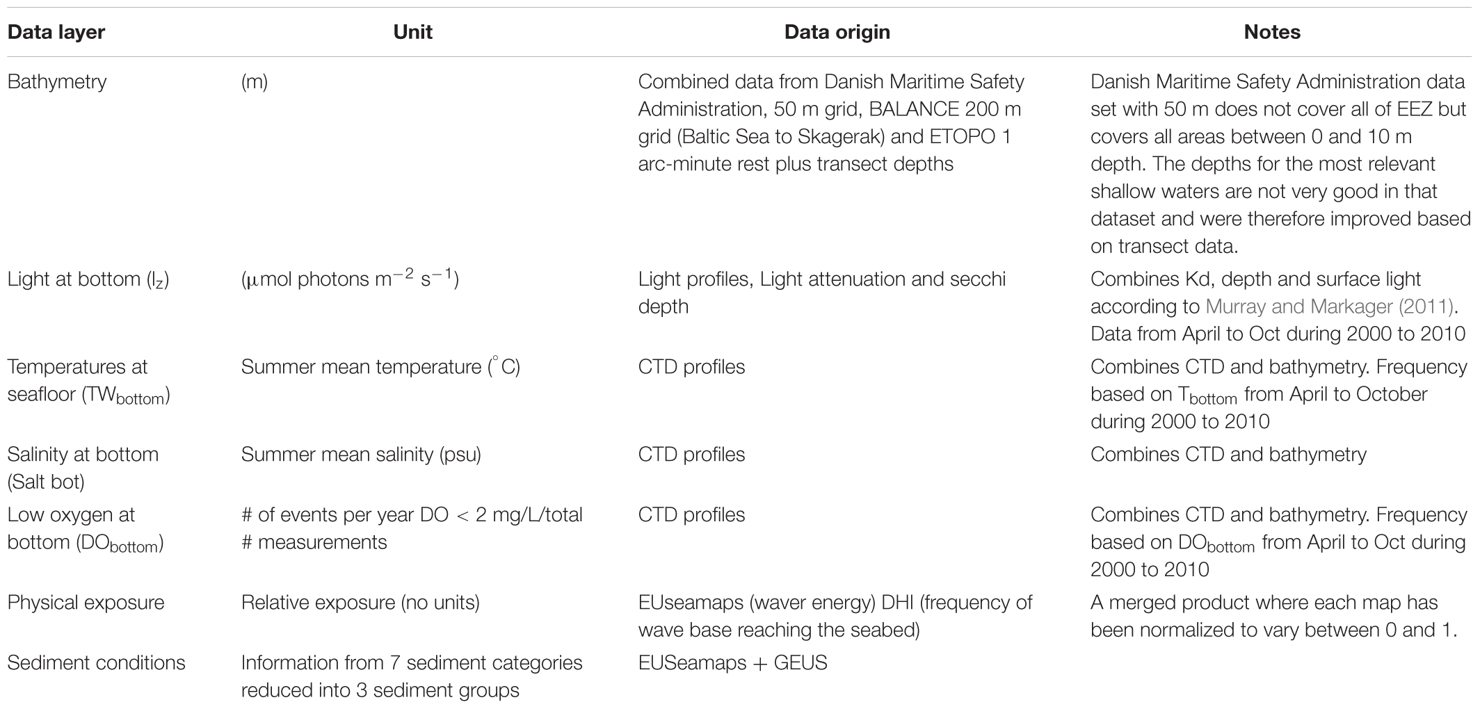
Table 1. Description of GIS data layers used to model the probability of eelgrass with a spatial resolution of 100 m × 100 m.

FIGURE 1

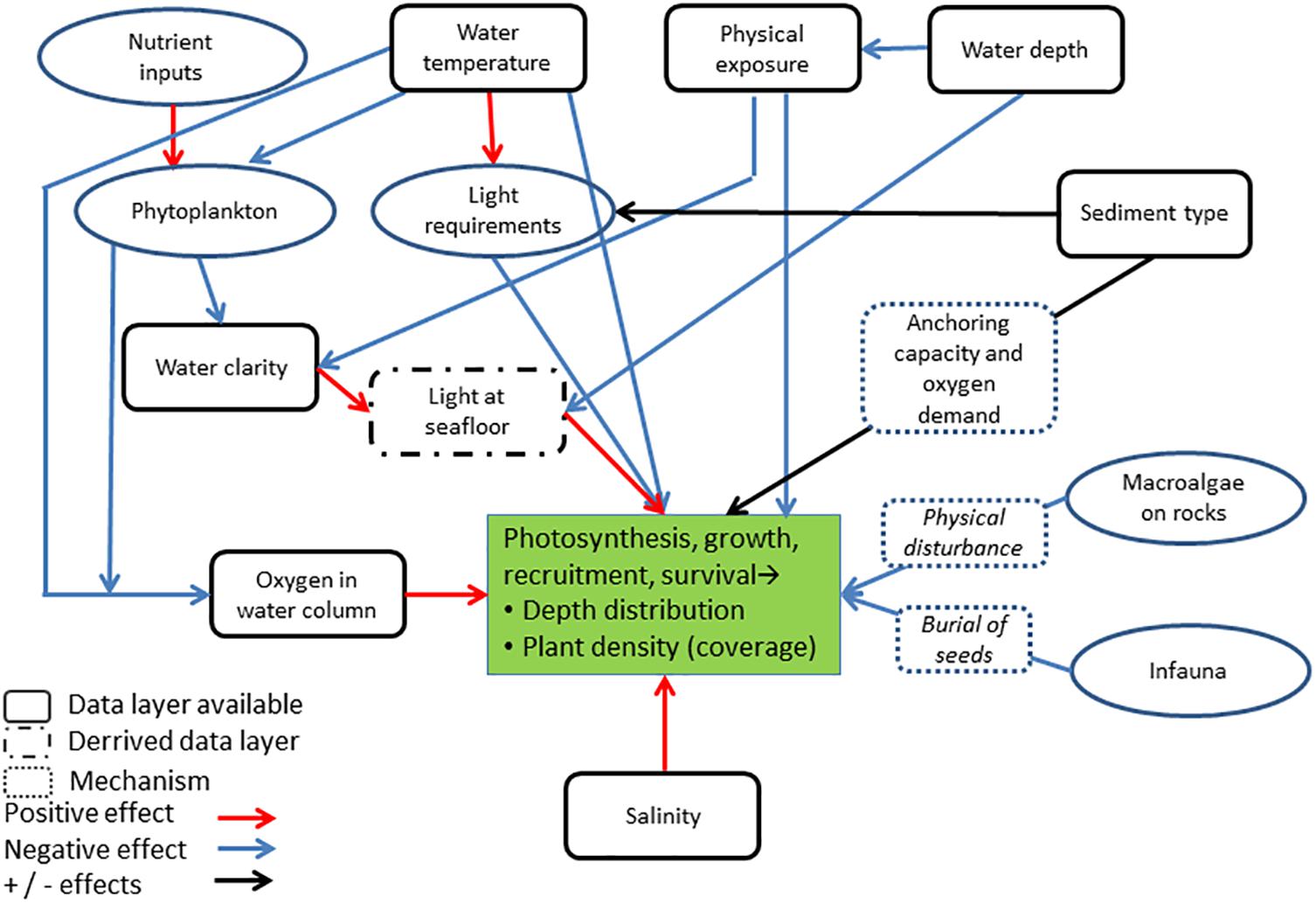
Figure 1. Conceptual model of linkages between abiotic and biotic conditions influencing the distribution of eelgrass plants in coastal waters. Increase in e.g., water clarity, oxygen concentration and salinity are expected to stimulate eelgrass distribution, whereas increases in e.g., physical exposure and water temperature are expected to limit eelgrass distribution. Conditions, for which we have access to nationwide data layers are marked as full black squares.

The GIS data layer on sediment characteristics was provided by the Geological Survey of Denmark and Greenland (GEUS) and consists of seven sediment classes: bedrock, hard bottom complex, gravel, sand, hard clay, muddy sand and mud. The sediment map has a scale of 1:250000. The coverage of the seafloor features varies within the area depending on the resolution of the different surveys (Cameron and Askew, 2011). The bathymetric maps for the Kattegat, inner Danish waters Danish estuaries and coastal zones were provided by the Danish Maritime Safety Administration at a nominal resolution of 50 m. Data on wave exposure and current velocities in the Wadden Sea and Western coastline of Jutland were provided by a hydrodynamic North Sea model (MIKE, DHI), whereas wave and current energy at the seafloor (hereafter named exposure) for the inner Danish waters and estuaries were provided from EUseamaps. Finally, as the spatial layers varied in resolution we aggregated data and exported these as gridded files with a spatial resolution of 100 m × 100 m.

Model Approach

Our modeling approach largely follows the recommendation by Hirzel and Le Lay (2008) for habitat suitability models. The model assumes that the coverage of eelgrass to a large extent reflects the suitability of the coastal habitats for eelgrass growth and survival. In addition, we assume that this overall suitability can be evaluated based on spatial information on a number of key environmental conditions for which we used the most suitable data.

The model consists of spatial data layers with environmental parameters (input data), which are either used directly in the eelgrass model or used to generate derived data layers, which are important for eelgrass growth (Figure 1). For each of the six environmental parameters we explored the relationship with in situ measured eelgrass coverage observed along transects. For a given spatial layer (e.g., bottom temperature) we extracted data on eelgrass coverage and the environmental value (here bottom temperature) on a pixel (50 × 50 m) level. The eelgrass coverage within the pixel was calculated as a mean value within the range of 0–100% coverage.

Correlations between eelgrass coverage and each of the six environmental conditions were modeled using relations derived from statistical analysis of the present data in combination with information from the literature on important thresholds, if available. The resulting data layers were then transformed into continuous index functions with a value between 0 (i.e., eelgrass growth/survival is impossible) and 1 (i.e., the parameter is not limiting eelgrass). Below, we briefly present the individual index functions. A detailed description of the index functions is available in the Supplementary Material.

Although habitat suitability models can be derived from discrete functionalities (Brooks, 1997), continuous non-linear functionalities (or smoothened threshold functions) are commonly used (Hirzel and Le Lay, 2008). Non-linear functions were chosen as these provided better fits and commonly used to estimate threshold values (Andersen et al., 2009).

Light Index

To develop a light index we used both light extinction coefficient (K_D) derived from light profiles and from Secchi depth converted to K_D following the method of Murray and Markager (2011). Here we parameterized the importance of the actually available light reaching the seafloor, rather than different indices of water clarity. First, we applied a standard equation (Beer’s law) to model bottom light levels (I_z) from measured light attenuation coefficients (K_D), light at the Sea surface (I_surface) and water column depth as:

$${\text{I}}_{\text{z}}={\text{I}}_{\text{surface}}\cdot {\text{e}}^{-{\text{K}}_{\text{D}}\cdot \text{depth}}\mathrm{\left(}\mathrm{1}\mathrm{\right)}$$

For I_surface, a constant value (384 μmol photons m^-2 s^-1), calculated as the mean daily light reaching the sea surface during summer (April to October) based on a 10 years data set from a measurement station at Højbakkegaard, Denmark. Rather than an arbitrary percent of surface light, we choose to evaluate the importance of light by comparing I_Z with the eelgrass coverage (in pct) observed at depth during a period from 1994 to 2010. This resulted in a data set of 7750 observations of pct cover and I_z (Supplementary Figure S2A). Data on light at depth represents cell sizes of 50 × 50 m compared to the mean eelgrass cover within the associated transects.

To deduce a pattern from the scattered cover vs. light data set (Supplementary Figure S2A), we calculated percent cover for a range of binned light data. This resulted in a bell shaped curve, which we then normalized to 1 (Figure 2). The light index model (red line in Supplementary Figure S2B) was parameterized using a combination of a polynomial function shown as a dotted blue line. Also, we included a threshold for the minimum light required for eelgrass plants to have a net positive growth (I_C). A first condition was therefore that I_Z should be >I_C for eelgrass to occur. The critical light level is known to vary as a function of water temperature and to display a strong seasonal variation, reflecting physiological acclimation of plants to prevailing light, temperature and nutrient conditions (Staehr and Borum, 2011). However, to simplify our light model we choose to apply an I_C value of 25 μmol photons m^-2 s^-1, which represents light requirements when summer mean water temperature ranges between 11 and 17°C with a median of 15°C (Staehr and Borum, 2011). Data show an apparent negative effect of high light levels (Supplementary Figure S2A), which we assume is an artifact driven by effects of other factors, such as physical exposure at shallow depth. Therefore, above the peak of the polynomial model (140 μmol photons m^-2 s^-1) we assigned a light index value of 1. Below the I_C value of 25 μmol photons m^-2 s^-1, the index value was set to zero. The light index model is described in Equation (2):

FIGURE 2

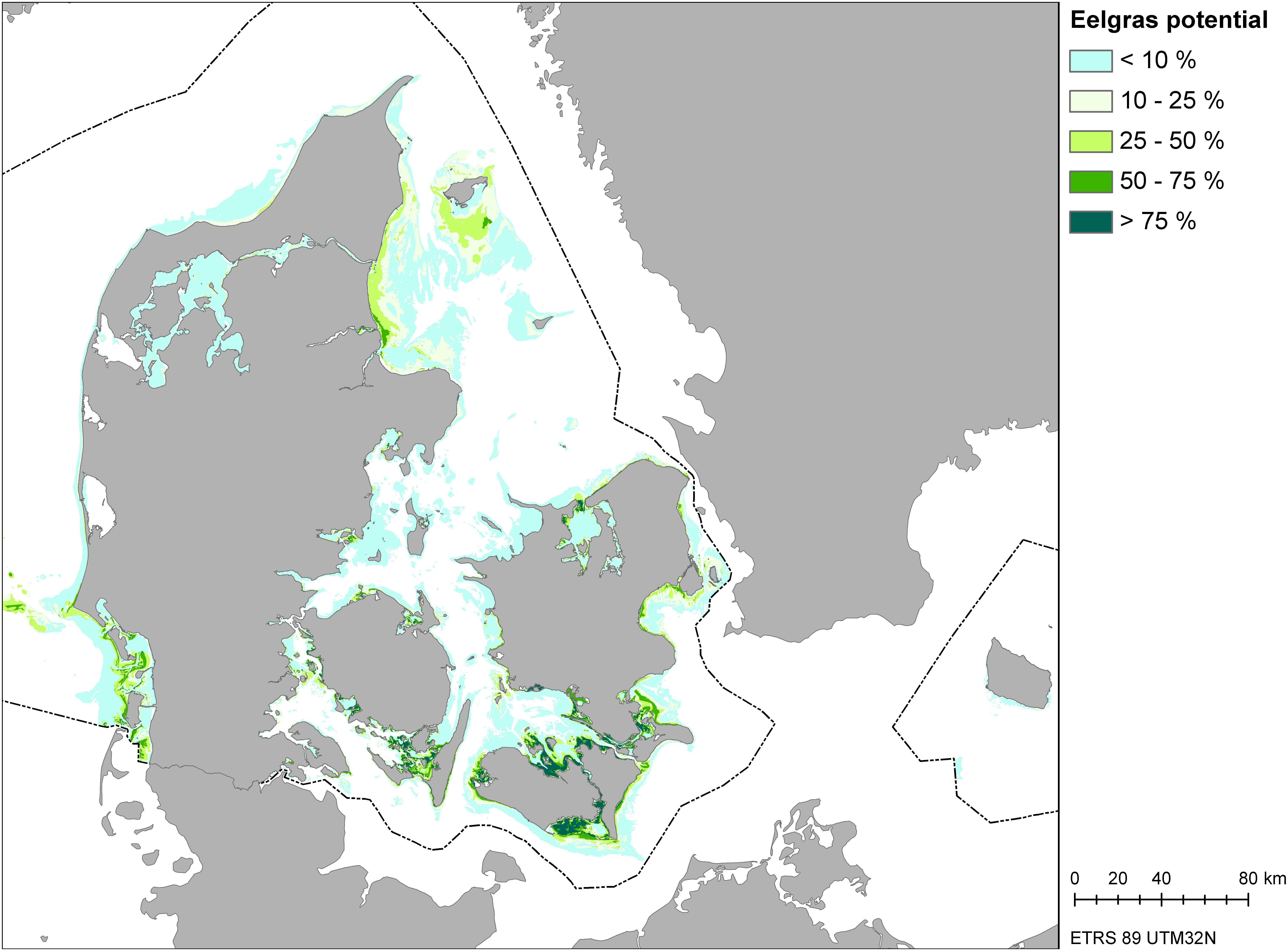
Figure 2. Map of eelgrass distribution potential area derived from spatial habitat modeling.

$$\begin{array}{ll}{\text{Light}}_{\text{index}}\text{=}\hfill & {\text{IF(I}}_{\text{Z}}{\text{ > 140 THEN 1, ELSEIF(140 > I}}_{\text{Z}}\text{ > 25}\hfill \\ \hfill & \text{THEN (0}{\text{.000000047*I}}_{\text{Z}}{}^{\text{3}}\text{-0}\text{.0000515}*{\text{I}}_{\text{Z}}{}^{\text{2}}\hfill \\ \hfill & \text{+ 0}{\text{.0135*I}}_{\text{Z}}),{\text{ELSEIF I}}_{\text{Z}}<\text{25 THEN 0))}\hfill \end{array}\mathrm{\left(}\mathrm{2}\mathrm{\right)}$$

Sediment Suitability Index

Sea bottom characteristics such as organic matter content affect the ability for eelgrass to become established, as well as the suitability for anchoring, growth and seed survival (Krause-Jensen et al., 2011; Flindt et al., 2016). In this GIS model, we applied a national wide sediment map with information on seven sediment categories (Cameron and Askew, 2011), which we merged into three substrate groups: (1) Mud, sandy mud, muddy sand and bedrock, (2) Sand (3) Hard bottom complex and gravel and coarse sand. To include information on sediment conditions as a determining factor for eelgrass distribution we assigned the following sediment index values ranging between 0 and 1 (unsuitable to suitable): Mud, sandy mud, muddy sand and bedrock (grp1) = 0.1; Hard bottom complex and gravel and coarse sand (grp3) = 0.5; Sand (grp2) = 1. The eelgrass coverage in these three groups is shown in Supplementary Figure S3. The final sediment index model is described in Equation (3)

$$\begin{array}{ll}{\text{Sediment}}_{\text{index}}\text{ =}\hfill & \text{IF (grp = 1THEN 0}\text{.1, ELSE}\hfill \\ \hfill & \text{(IF GRP = 2 THEN 1, ELSE 0}\text{.5))}\hfill \end{array}\mathrm{\left(}\mathrm{3}\mathrm{\right)}$$

Physical Exposure Index

Waves and tides limit eelgrass distribution especially in shallow waters where bottom exposure is most pronounced. To parameterize the effect of the physical exposure on eelgrass cover, we combined two data sources which both have weaknesses or data gaps in sub regions: (1) a map of the frequency with which the wave base reaches the bottom; produced by DHI covering the Danish waters without Limfjorden and (2) an EUSeaMap wave energy map (Log transformed) covering the North Sea including Limfjorden and the southwestern Baltic Sea but not the waters around Bornholm. Before combining the two layers, they were normalized.

Comparing the modeled exposure levels with eelgrass coverage on a pixel basis (5505 observations), showed that eelgrass coverage declined strongly when the normalized physical exposure exceeded a value around 0.2 (Supplementary Figure S4A). To parameterize the effect of physical exposure we applied a function, which represents the red line in Supplementary Figure S4B. Below the cut off value of 0.2, exposure levels are considered to be sufficiently low to enable full coverage of eelgrass, providing an index value of 1. In parallel to the reasoning conducted for eelgrass cover as a function of light, we interpreted that the apparent decline in eelgrass cover at low levels of physical exposure is largely due to deeper water where light levels limit distribution. The final exposure index model is described by Equation (4).

$$\begin{array}{ll}{\text{Exposure}}_{\text{index}}\text{ =}\hfill & \text{IF ((exposure > }0.2\text{) THEN}\hfill \\ \hfill & \text{(20 * EXP (}-\text{15 * exposure)), ELSE 1)}\mathrm{\left(}\mathrm{4}\mathrm{\right)}\hfill \end{array}$$

Temperature Index

To develop a temperature index, we made a map of summer mean (April to October) bottom water temperatures by interpolating data from CTD profiles. These modeled bottom temperature data were then combined with the gridded transect observation values (7006 observations). A comparison of eelgrass cover and bottom temperatures in the gridded cells are shown in Supplementary Figure S5A. This resulted in a bell shaped curve somewhat similar in shape to what has previously been shown in experimental studies (Nejrup and Pedersen, 2008; Staehr and Borum, 2011). To deduce a pattern from the scattered cover vs. water temperature plot (Supplementary Figure S5A) we calculated percent cover for a range of binned temperature data, which we then normalized to range between 0 and 1 (Supplementary Figure S5B). The temperature index model was parameterized using a polynomial function (Equation (5)):

$$\begin{array}{ll}{\text{Temp}}_{\text{index}}\text{ =}\hfill & -0.006079{\text{ * Tw}}^{\text{4}}\text{ + }0.3074*{\text{ Tw}}^{\text{3}}\hfill \\ \hfill & -5.7604{\text{ * TW}}^2\text{ + }47.587\text{ * Tw}-146.49\hfill \end{array}\mathrm{\left(}\mathrm{5}\mathrm{\right)}$$

where Tw is the mean summer bottom water temperature.

Oxygen Index

We compared eelgrass coverage at local sites with corresponding oxygen concentrations, obtained from oxygen depth profile measurements within the national monitoring program. As we did not have high frequency continuous oxygen data available, we used monitoring data to determine the frequency of low oxygen concentrations (<2 mg/L) at the sea floor during the summer growth season (April to October). These frequencies of low oxygen data were then combined with the gridded transect observation values providing 5576 observations (Supplementary Figure S6A). We interpret the low oxygen frequency data as an information layer reflecting the sensitivity of eelgrass to low oxygen conditions. According to this, we expect low coverage of eelgrass due to mortality and poor performance in areas with high occurrence/frequency of low oxygen.

The negative impact of low oxygen conditions was included in the model by an oxygen index function (Equation (6)):

$${\text{Oxygen}}_{\text{index}}=\text{ 1 }-\text{ ((}1\text{/(}1\text{ + EXP( }-{\text{(DO}}_{\text{Low}}\text{ * }20\text{) + }6\text{))))}\mathrm{\left(}\mathrm{6}\mathrm{\right)}$$

Where DO_Low is the relative frequency (ranging between 0 to 1) of days per summer (May to September) with observed DO at depth below 2 mg/L (Supplementary Figure S6B).

Salinity Index

An experimental study of the effect of salinity on several eelgrass performance parameters showed that optimal salinities range between 10 and 25 psu, with increased mortality and lowered performance at low salinities and moderate effects at high salinities (Nejrup and Pedersen, 2008). The potential success of eelgrass is therefore expected to be reduced in areas of low salinity, but remains only weakly affected by high salinities. To evaluate this further, we compared eelgrass cover at 7750 sites with summer mean bottom salinities (Supplementary Figure S7A). The comparison does suggest a somewhat bell shaped dependency/effect of salinity. Since no experimental evidence exists for the apparent negative effect of high salinities, we expect that this arises from other confounding factors such as higher levels of exposure in high saline waters and lower light levels at larger depths where salinities usually increase during stratification.

The effect of low salinity on plant performance and survival was included in the model by a salinity index function (Equation (7); Supplementary Figure S7B):

$${\text{salinity}}_{\text{index}}=\text{ IF ((salt < }7\text{ THEN (EXP(}1\text{ * (salt-}7\text{))), ELSE 1))}\mathrm{\left(}\mathrm{7}\mathrm{\right)}$$

Where salt is the bottom water salinities determined from CTD profiles and interpolated to the corresponding eelgrass monitoring sites.

Eelgrass Habitat Model

We tested different combinations of the six environmental index maps to produce a national map of the potential habitat occupied by eelgrass plants in Danish coastal waters. In all cases the environmental index maps were combined to produce an eelgrass habitat map with values ranging from 0 to 1, reflecting 0–100% expected presence of eelgrass. As suggested by Hirzel and Le Lay (2008) we tested different combination of the data layers in our GIS model. These varied in the prioritization of the importance of the different data layers, especially light and physical exposure which we expected to be of greater importance. However, a comparison between the measured and modeled cover showed that a simple multiplicative model, which gives equal importance to each data layer (Equation (8)), was best:

$$\begin{array}{ll}{\text{Eelgrass}}_{\text{index}}\text{ =}\hfill & {\text{Light}}_{\text{index}}{\text{ * Exposure}}_{\text{index}}{\text{ * Temp}}_{\text{index}}\hfill \\ \hfill & {\text{*Oxygen}}_{\text{index}}{\text{ * Sediment}}_{\text{index}}\hfill \\ \hfill & {\text{* salinity}}_{\text{index}}\hfill \end{array}\mathrm{\left(}\mathrm{8}\mathrm{\right)}$$

Conversion of parameter layers to index layer and calculation of the eelgrass model index was done on the 100 m × 100 m resolution raster layers with arcpy in ArcGIS 10.3.

Model Performance

To assess the performance of the GIS probability map (Zost GISmodel), we performed a validation using independent datasets of eelgrass cover from recent years (Table 2). One data set (Zost Map2012) covered three selected study areas encompassing 292 km² within 0–5 m depth. The areas were Nibe-Gjøl Bredning in Limfjorden, Saltholm including the Zealand coast facing Saltholm, and the South Funen Archipelago. The eelgrass coverage in these three areas were derived from a pixel based supervised image analysis of aerial SOP from 2012 performed with linear discriminant analysis of color bands (red, green, blue) involving two classes, ‘eelgrass’ and ‘bare sand’ (Ørberg et al., 2018). Indeed, other marine vegetation was most likely classified as eelgrass, but the mapping was performed in areas with eelgrass as the dominant vegetation type. A second data set used to validate the GIS modeled distribution was based on NOVANA monitoring transects from 2012 covering Nibe-Gjøl Bredning, Saltholm, South Funen (Zost Moni2012) and all Danish coastal waters also in 2012 (Tot Zost Moni2012). Finally, we used a high-resolution ground truth data set from Mariager Fjord (Zost Obs2009) (Clausen et al., 2015).

TABLE 2

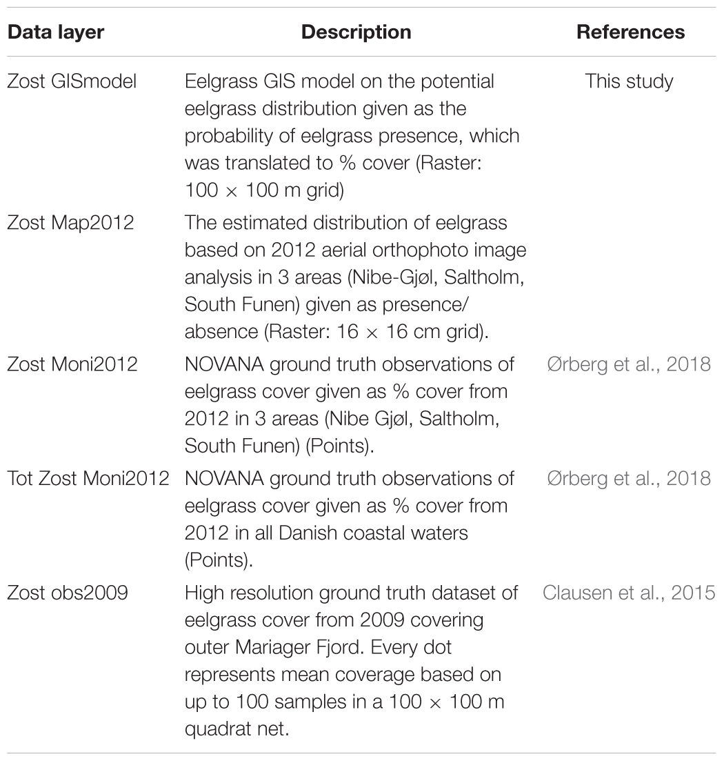
Table 2. Data layers used in the validation of the map derived from the GIS model predicting potential distribution of eelgrass in Danish coastal waters.

Prior to validation of the GIS model coverage with SOPs and monitoring data points, all data layers were converted into raster’s, matching the bathymetry grid size (50 m × 50 m). Hence, the Zost Map2012 values (presence = 100, absence = 0) were averaged within each grid, resulting in values ranging between 0 and 100. Similarly, the Zost Moni2012 and Tot Zost Moni2012 data points (pct cover) were averaged within each grid and the Zost GISmodel was converted from a 100 m × 100 m grid to a 50 m × 50 m grid. We did not average the Zost Obs2009 data within each grid because there was approximately one data point per pixel.

With equal grid sizes of 50 m × 50 m, we translated the reshaped data layers into presence/absence data by the following rules: Values <10 define the absence of eelgrass, and values ≥10 define the presence of eelgrass. Hereafter, we calculated the accuracy of the Zost GISmodel displayed in confusion matrices. To identify areas of particularly low/high accuracy compared to the Zost Map2012, we created maps displaying the agreement/disagreement between Zost GISmodel and Zost Map2012 for the three selected areas with shallow water. Similar to recent evaluations of eelgrass distributions, we used 10% cover of eelgrass as a threshold for defining areas where eelgrass meadows are present (Bostrom et al., 2014).

Importance of Environmental Conditions

We applied two different approaches to evaluate the importance of variations in the applied environmental conditions. These consisted of a statistical analysis and a sensitivity analysis. The statistical analysis investigated the importance of environmental variables for areas showing disagreement between predicted and measured eelgrass cover. Here we defined three groups of data: Agreement (grp 0) between predicted (Zost GISmodel) and observed (Zost Map2012); Prediction of eelgrass presence while Zost Map2012 show no eelgrass (-1) or vice versa (1). We applied a non-parametric Kruskal–Wallis test and a multiple comparison post hoc test (nemenyi from Desctools) in R to test whether environmental parameters differed significantly between the three groups. We only studied parameters for which eelgrass habitat requirements and thereby thresholds are less understood (physical exposure, oxygen, temperature, and salinity) compared to the basic requirements, such as light and sediment type.

To investigate the sensitivity of the eelgrass distribution (km²) calculated by the GIS model, we performed a series of model runs where each input data layer (except the sediment map) was varied separately between -20 and + 20%. To gain information about possible regional differences in the sensitivity of the selected variables, we divided the Danish waters into three regions, covering Limfjorden, the Kattegat and the Eastern Baltic Sea (Supplementary Figure S8).

Results

Based on the eelgrass spatial habitat model, we produced a nationwide map (Zost GISmodel) of the potential distribution area of Danish eelgrass meadows (Figure 2). From this map, we calculated the total potential eelgrass distribution area in Danish waters to be 2204 km² (probability >10% × pixel size × pixel numbers). Furthermore, we compared the Zost GISmodel with ground truth observations and orthophoto mapping of eelgrass cover from recent years.

Model Validation With Monitoring Data and SOP

As an initial step, we calculated the accuracy of the Zost GISmodel and the SOP based map (Zost Map2012) compared to in situ observations (Zost Moni2012) on eelgrass cover in three shallow areas (a total of 538 pixels). The GIS modeled distribution showed an accuracy of 67.1% (Table 3A). In comparison, the Zost Map2012 displayed a higher accuracy (80.3%) (Table 3D), thereby serving as a relevant map to validate Zost GISmodel on a larger spatial scale (Table 3B). While the accuracy of Zost Map2012 varied between the three areas (Figures 3B–D) the level of agreement with in situ data was overall high and stable across all depth intervals (Figure 3A). In comparison, the level of agreement of the Zost GISmodel was lower and tended to increase with depth (Figure 4A). The low accuracy, caused by the Zost GISmodel underestimating eelgrass distribution at shallower depths, was most pronounced in Nibe-Gjøl Bredning (Figure 4B). In comparison, both the Zost GISmodel and the SOP map overestimated eelgrass distribution compared to in situ observations in the very shallow areas (0–1 m) at Saltholm and South Funen (Figures 3C,D, 4C,D).

TABLE 3

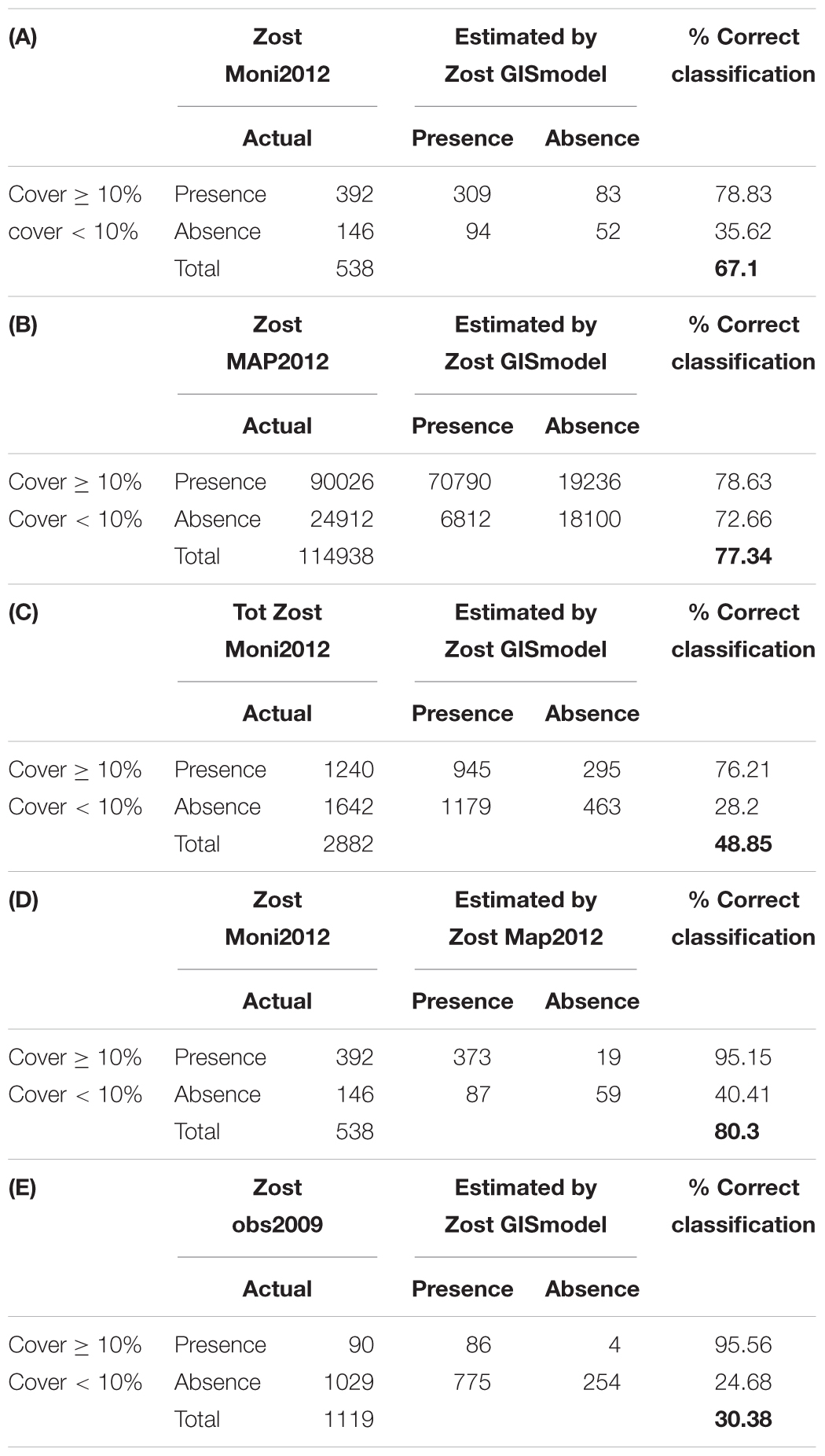
Table 3. Confusion matrices comparing classification results of the GIS model (Zost GISmodel) with (A) in situ monitoring data in three smaller areas (Zost Moni2012); (B) 2012 aerial orthophoto image analysis in three smaller areas (ZOST MAP2012); (C) in situ monitoring data in all monitored areas in 2012 (Tot Zost Moni2012). In (D) we compare results from in situ monitoring and orthophotos in 2012 and finally in (E) we evaluate the GIS model performance against high-resolution from Mariager fjord in 2009. For each pixel, data were categorized into presence or absence of eelgrass, while less than 10% cover was considered as absence. Correct classification gives the % of pixels classified correctly to each category and in total.

FIGURE 3

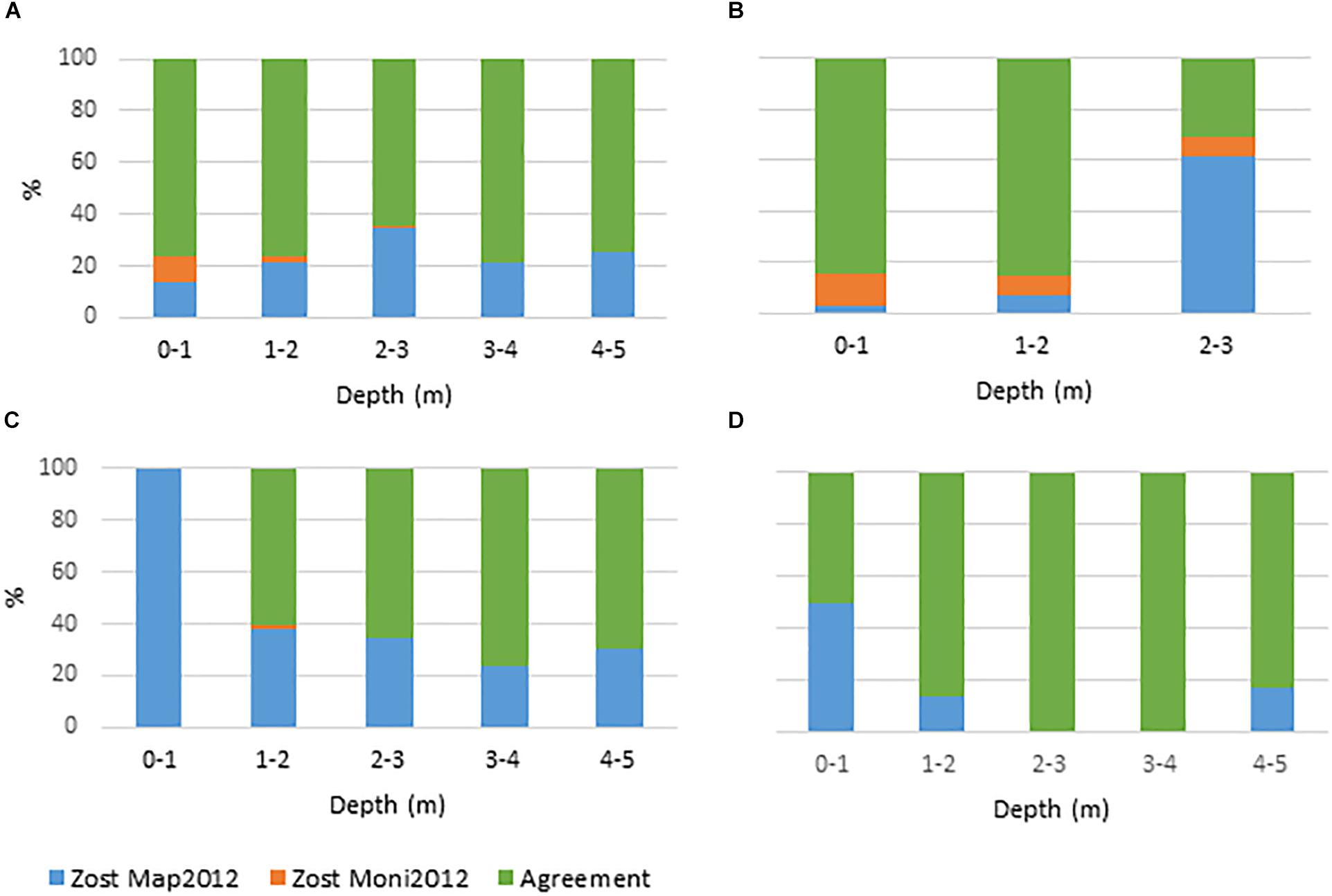
Figure 3. Agreement and disagreement (%) between Zost Map2012 and Zost Moni2012 across depth intervals for Nibe Gjøl bredning, Saltholm, and South Funen. (A) All areas combined, (B) Nibe Gjøl bredning, (C) Saltholm, and (D) South Funen. Green displays the percentage of all pixels where the models agree. Orange and blue display the disagreement between models. Blue show the percentage of pixels where Zost Map2012 displays the presence of eelgrass when Zost Moni2012 displays the absence of eelgrass. Orange is vice versa.

FIGURE 4

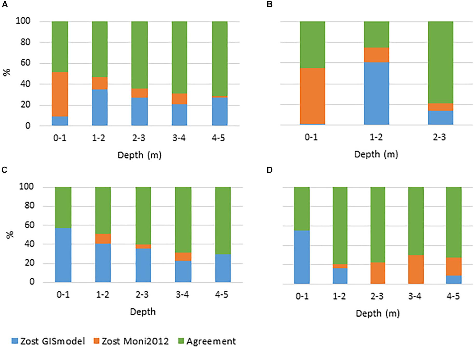
Figure 4. Agreement and disagreement (%) between GIS habitat model (Zost GISmodel) and Monitoring data (Zost Moni2012) across depth intervals for Nibe Gjøl bredning, Saltholm, and South Funen. (A) All areas combined, (B) Nibe Gjøl bredning, (C) Saltholm and (D) South Funen. Green displays the percentage of all pixels where the models agree. Orange and blue display the disagreement between models. Blue shows the percentage of pixels where Zost GISmodel displays the presence of eelgrass when Zost Moni2012 displays the absence of eelgrass. Orange is vice versa.

A direct comparison of the eelgrass distribution between the Zost GISmodel and the SOP map resulted in an overall agreement of 77.3% (a total of 114938 pixels) in the three case study areas (Table 3B and Figures 5A–D). Disagreements between the Zost GISmodel and the SOP maps in 2012 were highest in the very shallow areas (38%). However, this decreased with depth, suggesting that the Zost GISmodel mainly underestimated eelgrass presence in the 0–1 m depth interval (Figure 5A), particularly around Saltholm (Figure 5C). The level of agreement/disagreement between the GIS modeled, SOP mapped and in situ monitored distribution of eelgrass were visualized in maps representing the three case study areas (Figure 6). While agreement between GIS and SOP maps dominate all three areas, they all have deeper zones where only in situ monitoring data indicate the presence of eelgrass.

FIGURE 5

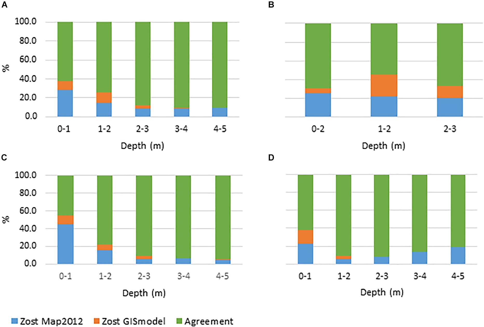
Figure 5. Agreement and disagreement (%) between GIS habitat model Zost GISmodel and the summer orthophoto map from 2012 (Zost Map2012) across depth intervals for Nibe Gjøl bredning, Saltholm and South Funen. (A) All areas combined, (B) Nibe Gjøl bredning, (C) Saltholm and (D) South Funen. Green displays the percentage of all pixels where the models agree. Orange and blue display the disagreement between models. Blue show the percentage of pixels where Zost Map2012 displays the presence of eelgrass when Zost GISmodel displays the absence of eelgrass. Orange is vice versa.

FIGURE 6

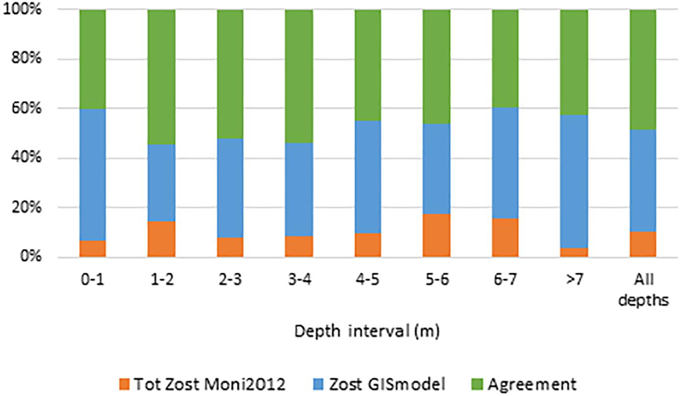
Figure 6. Agreement and disagreement (%) between Zost GISmodel and Tot Zost Moni2012 across depth intervals for all Danish coastal waters. Green displays the percentage of all pixels where the models agree. Orange and blue display the disagreement between models. Blue show the percentage of pixels where Zost GISmodel displays the presence of eelgrass when Tot Zost Moni2012 displays the absence of eelgrass. Orange is vice versa.

In addition to the three case study areas, we evaluated the nationwide accuracy of the Zost GISmodel against an in situ data set representing all Danish coastal waters (Tot Zost Moni2012). We found an overall accuracy of 48.9% of the modeled eelgrass cover (a total of 2882 pixels) (Table 3C). While there was a high agreement (76.2%) in areas where in situ data show presence of eelgrass, the agreement was much lower (28.2%) in areas where in situ data show less than 10% coverage of eelgrass (Table 3C), suggesting that the Zost GISmodel most often overestimates the eelgrass cover. The level of disagreement between in situ observations and the Zost GISmodel was consistent throughout all depths (Figure 7). A similar comparison with high-resolution in situ observations from Mariager fjord 2009 (Zost Obs2009, Supplementary Figure S9) gave an overall accuracy of the Zost GISmodel of 30.4%, which also highlights that the agreement is lowest in areas where in situ data show less than 10% coverage of eelgrass (Table 3E).

FIGURE 7

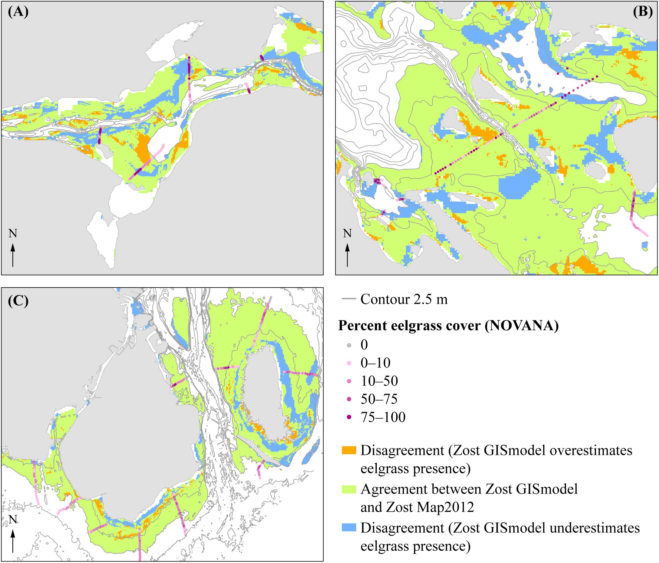
Figure 7. Map of areas of agreement and disagreement between the summer orthophoto maps (Zost Map2012) and the GIS habitat map (Zost GISmodel). (A) Nibe Gjøl bredning, (B) South Funen and (C) Saltholm. Green displays where the models agree. Orange and blue display the disagreement between models. Blue shows where Zost Map2012 displays the presence of eelgrass when Zost GISmodel displays the absence of eelgrass. Orange is vice versa. Ground truth data from NOVANA 2012 of eelgrass cover are annotated with points grading from gray to dark purple, where gray = 0% cover and dark purple = 100% cover. Gray line marks 2.5 m depth contour line.

Importance of Environmental Conditions

Comparing monitored eelgrass data with the geographically interpolated environmental data layers, showed that eelgrass coverage was higher in areas characterized by high light levels, shallow depth, high wave exposure, low frequency of oxygen depletion and higher temperatures (Table 4). Although the dependency of eelgrass cover was far from linear (see Supplementary Material), we expect the GIS model to perform overall well in such areas. As a first approach to investigate the importance of environmental conditions for the accuracy of the GIS model, we calculated the levels of three of the selected environmental parameters (exposure level, mean summer temperature and salinity) in areas with agreement and disagreement with the orthophoto mapped eelgrass areas in 2012. For areas of disagreement, we found that we found that mean exposure level, mean summer temperature and mean salinity were all significantly higher (p < 0.0001) higher compared to areas of agreement between the Zost GISmodel and SOP validation data. In areas of disagreement, exposure was higher by 0.063 exposure units, mean summer temperature was higher by 0.17°C, and mean salinity was higher by 1.16 psu. As disagreement may also depend on habitat characteristics, we further tested whether all three possible outcomes [i.e., 0 = Agreement, 1 = the orthophoto map (Zost Map2012) predict eelgrass while the GIS model does not, -1 = GIS model predict eelgrass while Zost Map2012 does not] differed in level/intensity of each environmental parameter. The exposure level differed between all groups with significantly higher exposure level in areas where the GIS model underestimated eelgrass coverage (Supplementary Table S1). Small, but significant differences in mean summer bottom temperature and salinity between the three groups were also apparent. This suggests that the GIS model is currently less reliable in areas where exposure levels are higher than 0.33 on the exposure scale, where mean summer temperatures are higher than 14.7°C and where salinity is higher than 15.1 psu. The correlation analysis of relationships between the applied environmental variables suggested that the high levels of wave exposure prevailed at shallow depths in both Kattegat, Limfjorden and the Baltic Sea regions (Table 4). Moreover, temperatures tend to increase toward shallow waters (except Limfjorden), while salinities increased with depth. Areas associated with higher light levels were, as expected, associated with shallower depth, and higher wave exposure, but lower frequency of low oxygen conditions.

TABLE 4

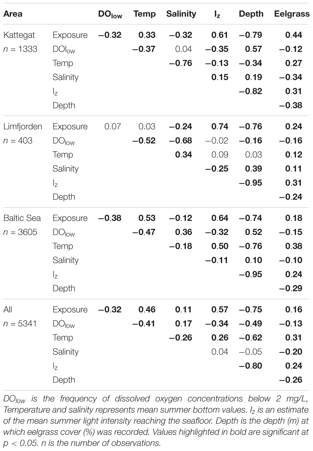
Table 4. Spearman correlation analysis of relationships between environmental variables used in the GIS model to estimate eelgrass coverage.

Varying the value of each environmental variable in each pixel between -20% and +20% relative to baseline conditions, provided a simple sensitivity assessment of the GIS model to the applied data layers and their parameterization of eelgrass suitability except for the sediment conditions. Comparing three regions, the Kattegat, Limfjorden and the Baltic Sea (Figure 8), we found a strong sensitivity in all areas to variations in light conditions. The modeled eelgrass area was also quite sensitive to changes in wave exposure, low oxygen conditions and low bottom water temperatures, while salinity did not appear to have any influence. Limfjorden was the most sensitive area for changes in light and wave exposure, but less sensitive to low oxygen conditions. All three regions were surprisingly sensitive to changes in temperature. However, while higher temperatures had a negative impact on eelgrass coverage in Limfjorden and the Baltic Sea, the sensitivity analysis suggested that the coverage would increase significantly in the Kattegat area with increasing temperatures (Figure 8).

FIGURE 8

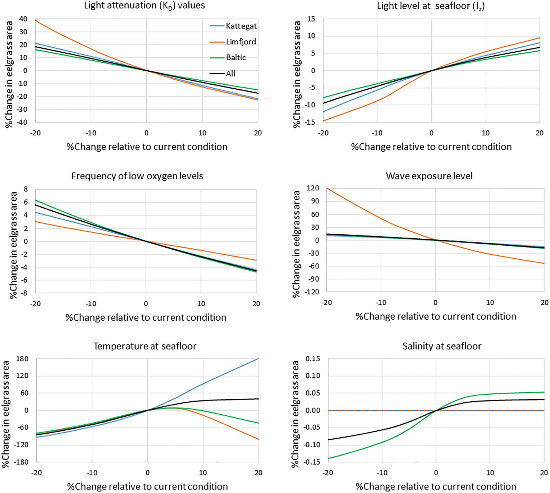
Figure 8. Assessment of the sensitivity of the GIS modeled eelgrass area to changes in environmental conditions. We compare three regions, the Kattegat, Limfjorden and the Baltic Sea region (see Supplementary Figure S8). The input value in each pixel was varied between -20% to +20% relative to baseline conditions. Sensitivity was assessed from changes in the potential eelgrass area relative to baseline.

Discussion

Model Performance

Applying different independent data sets (in situ monitoring data and SOPs) to validate the GIS model showed overall good agreement with the GIS model. In addition, the GIS model performance seems reasonable when comparing with previous modeling efforts (Krause-Jensen et al., 2003; Bekkby et al., 2008). However, model performance varied greatly between geographical areas, and the model did not perform well in predicting small-scale distribution patterns. It should be noted that the GIS model aims to provide estimates of the potential distribution and cover of eelgrass given a combination of key environmental conditions, for which we have spatial data available at the national scale. The overall (national scale) good agreement between model results and data indicate that the model contains the main controlling parameters determining eelgrass distribution, whereas factors not included in the model (e.g., drifting macroalgae, epiphytes and bioturbation) locally may play a significant role for eelgrass growth and distribution.

The GIS model estimated a total area of eelgrass with 10% coverage or more to be 2204 km^2, which is close to the range recently estimated by Bostrom et al. (2014) (ca. 1400–2100 km²). In agreement with the empirical data on which the GIS model was parameterized, our model validation provided high eelgrass coverage in areas characterized by shallow sheltered waters such as the South Funen area. This area is also know to host many water birds which depend on eelgrass as a food source (Clausen, 2000).

Under-estimation of eelgrass presence at shallower depth in some areas such as Nibe-Gjøl Bredning suggests that the environmental thresholds for eelgrass presence in the GIS model may be too conservative. However, in other areas such as Saltholm, both the GIS model and the SOP maps indicated higher eelgrass distribution compared to in situ monitoring. While higher estimates of eelgrass cover by the GIS model may indicate potential areas of near future colonization, deviations may also reflect inaccuracies in the in situ data or simply inadequacies in the GIS model. Interestingly, the shallow areas around Saltholm (0–1.5 m) are known to be dominated by other rooted macrophytes such as Ruppia sp. rather than eelgrass (Noer and Petersen, 1993; Krause-Jensen and Christensen, 1999). Concerning inaccuracies in the in situ data, our comparison of the GIS model with a high-resolution data set from Mariager Fjord, showed that the GIS model overestimated the current distribution of eelgrass. However, similar to Saltholm, the vegetation at shallow depths in Mariager Fjord was dominated by Ruppia species (Clausen et al., 2015). Overestimation of eelgrass cover by both the GIS model and the SOP maps at shallow depth suggest that they are not capable of distinguishing between different rooted macrophytes such as Ruppia sp. and eelgrass. Future work should investigate specific habitat requirements and possibilities to distinguish RGB signals of different species. Incorporating biotic parameters, such as interspecific competition and foraging, would likely improve the GIS model. Currently, we must acknowledge that both the SOP maps and the GIS model to some extent estimate coverage of not just eelgrass, but rooted macrophytes in general. While the GIS model compares reasonably well with the overall trends in eelgrass cover, the current coarse resolution makes it inadequate to thoroughly investigate conditions determining the distribution and size of eelgrass patches. Such analysis would be possible with the detailed SOP’s which gives information at 10–20 cm scales in shallow waters. While this would be interesting, this was outside the scope of this current study, which primarily focuses on developing a model that enable us to understand changes at the landscape scale.

Perhaps a large source of uncertainty and error in our GIS habitat suitability model is the use of extrapolation of pelagic data (oxygen, temperature, salinity, light attenuation) from central stations in deeper waters into the nearshore shallow waters. Unfortunately, there are very limited datasets available for Danish waters for the required parameters. Aggregation of a new nationwide coastal dataset was therefore only possible by extrapolation. One key thing to be noted is that the central stations are not really deep, as Danish waters are quite shallow in general with depths typically of less than 20 m at the central sampling stations. Comparisons with a limited data set from the shallow Roskilde Fjord suggests that measurements in the upper part of the water column represented conditions in the shallow sites reasonably well (data not shown). In addition, the station grid is quite dense and as the calibration of the GIS model was done with the extrapolated values, the actual values have less importance. Furthermore, the morphometry and environmental conditions vary substantially in the Danish coastal zone (Conley et al., 2000), hence any error associated with extrapolation will not be systematic.

Importance of Environmental Conditions

In agreement with recent spatial predictive probability models, our GIS model also predicts that the probability of finding eelgrass is highest in shallow and sheltered areas (Bekkby et al., 2008), where light conditions are within the optimal range for the species (Canal-Vergés et al., 2016; Flindt et al., 2016; Kuusemäe et al., 2016). These areas were also highly represented by independent data sets based on in situ monitoring and SOP’s. Comparing levels of the environmental variables in areas with agreement and disagreement with the independent validation data sets indicated that disagreement was higher in areas with elevated levels of exposure, as well as temperature and salinity, although the latter were significantly less important. Underestimation by the GIS model therefore mostly occurred in areas with high exposure levels, suggesting a high sensitivity to this variable. A recent model of eelgrass coverage in two Danish fjords, similarly showed that physical exposure, in terms of waves has a strong negative impact on eelgrass growth and distribution (Kuusemäe et al., 2016). The physical exposure data layer applied in our analysis had to be merged from two normalized data sets to cover the entire Danish area. This disabled us from using a physical unit which would have been preferable. However, as the GIS model was calibrated with the derived data, the actual values have less importance. Our highest concern was to obtain a homogeneous data set. A nationwide detailed map of physical exposure should be developed for future models of eelgrass habitats.

A sensitivity analysis of environmental variables underlines that light is a strong determinant of the depth distribution of eelgrass in the Danish coastal waters. This agrees well with the established statistical relationship between maximum eelgrass colonization depth and water transparency, as measured by K_D or Secchi depth (Nielsen et al., 2002; Carstensen et al., 2013). The applied light dependency in our GIS model included a minimum light requirement threshold value which is known to exist for eelgrass (Staehr and Borum, 2011). However, our data set did not support the importance of such a clear minimum light threshold for the coverage of eelgrass. Rather, eelgrass coverage decreased gradually toward zero as light approached zero. Different studies have shown that seagrass light requirements depend on the environmental conditions and are higher in turbid waters (Duarte et al., 2007) and in areas with higher sediment organic matter content (Kenworthy et al., 2014) compared to seagrasses growing in clearer waters. The apparent absence of such a minimum threshold limit, indicated by our data, suggests that we have underestimated the in situ light levels at the depth limits. Alternatively, interpolating over a large pixel size (100 × 100 m) caused an overestimation of eelgrass coverage.

Both the correlation and sensitivity analysis suggested high importance of temperature for regulating the cover of eelgrass in Danish waters. Temperature affects eelgrass performance directly via effects on photosynthesis, respiration (Staehr and Borum, 2011), growth and survival (Nejrup and Pedersen, 2008), hence affecting eelgrass distribution through several processes (Bostrom et al., 2014). All enzymatic processes related to plant metabolism are temperature dependent (Drew, 1978), and specific life cycle events, such as flowering and germination, are often strongly dependent on temperature (De Cock, 1981; Phillips et al., 1983; Blok et al., 2018). In addition, biogeochemical processes are also affected by temperature, thereby influencing the interaction between plant, sediment and water column. Furthermore, temperature impacts seagrass performance by lowering water column oxygen content, increasing the oxygen diffusion coefficient, increasing respiration (Borum et al., 2006) and greatly reducing plant tolerance to anoxia (Pulido and Borum, 2010). Effects of temperature on eelgrass performance have previously been described by a bell shaped temperature dependency with optimum temperatures around 20°C (Nejrup and Pedersen, 2008; Staehr and Borum, 2011). In this study, we also applied a bell shaped curve, but by setting a much lower optimum temperature (15°C). This is because we used the mean summer temperatures at the local sites, calculated as a mean of ca.10–20 measurements during April to October at each eelgrass site. The fact that our data suggests maximum coverage at 5°C below the normal temperature optimum, implies that high mean temperatures are related to much higher maximum temperatures, which can extend beyond 20°C. The sensitivity analysis showed surprisingly high sensitivity to changes in the temperature layer. Lowering the bottom temperatures compared to current conditions were all associated with lower cover, and except for the Kattegat area, elevating the temperatures resulted in substantial declines in eelgrass. Given the ability of eelgrass to grow successfully in waters with significantly lower and higher temperatures (Bostrom et al., 2014), we find it unlikely that the occurring increases in summer water temperatures (Riemann et al., 2016) per se will cause major shifts in eelgrass coverage in Danish waters. While temperature is undoubtedly an important parameter affecting growth and distribution of eelgrass, the high sensitivity documented by our model, indicates that the temperature parameterization should be optimized by including better data on the high temperature conditions experienced by the plants. We recommend that future spatial modeling of large-scale eelgrass coverage applies data on frequency of temperatures above optimum. This should reduce the co-variation of mean summer temperatures with other important regulating factors (depth, light, salinity, exposure).

The effects of salinity on eelgrass performance have received relatively little attention despite its potential relevance particularly in estuarine environments, which typically are strongly affected by variations in freshwater inputs from precipitation, rivers and surface run-off (Conley et al., 2000). Coastal waters and estuaries, in particular, are prone to large and sometimes rapid changes in salinity. Eelgrass is a euryhaline species, and is found in both low saline systems (2–5%) such as rivers mouths, the inner estuaries and in waters of high salinity (35–40%) (Nejrup and Pedersen, 2008; Bostrom et al., 2014). It could therefore be argued that salinity is a relatively “unimportant” factor for the distribution of eelgrass, as also suggested by the sensitivity analysis in this study. However, eelgrass does not thrive equally well at all salinities and previous studies have shown that both survival and growth, as well as reproduction and seed germination are affected at extreme salinity (Phillips et al., 1983; Bostrom et al., 2014).

Low oxygen concentrations are also known to reduce growth and increase eelgrass mortality and have been associated with low coverage of eelgrass (Krause-Jensen et al., 2011; Canal-Vergés et al., 2016). Even short periods (12 h) of exposure to anoxic conditions reduce eelgrass performance whereas 24 h reduces the growth and kills eelgrass leaves (Pulido and Borum, 2010). The effect of anoxia is exacerbated when temperatures reach 25°C and severe at 30°C (Pulido and Borum, 2010). As temperature itself affects oxygen levels through changes in solubility of oxygen and anabolic oxygen demand, some covariation between temperature and oxygen can be expected, which we have currently not taken into account in our sensitivity analysis. In our study, we included information on oxygen sensitivity through a data layer representing the summer mean frequency of oxygen conditions below 2 mg/L. The applied oxygen index allowed us to exclude areas with too frequent anoxic events as previously done in other studies (Canal-Vergés et al., 2016; Flindt et al., 2016). As expected, eelgrass coverage showed a decreasing trend with increasing frequency of low oxygen in all areas. In addition, the sensitivity analysis suggested a significant influence of improved oxygen conditions for areal coverage of eelgrass suggesting that our parameterization was useful.

The long history of eutrophication has led to organically enriched sediments with low critical shear stress, which is easy to resuspend, providing poor anchoring for eelgrass (Krause-Jensen et al., 2011; Canal-Vergés et al., 2016). For our large-scale model, we applied a data layer that originally included seven sediment groups. However, the resolution is rather coarse and the seven categories do not contain specific information for eelgrass suitability, such as organic matter content, and furthermore are not exclusive but include areas dominated by other substrate types. Accordingly, the group defined as mud and bedrock contains significant areas with, e.g., sand and gravel which are suitable for eelgrass plants. Considering these limitations, we reduced the original seven sediment groups into three surrogate sediment groups, which differed in the observed coverage of eelgrass (Supplementary Figure S3). While sediment conditions are most likely very important for determining the possible coverage of eelgrass, limitations in the current classification and the coarse resolution of the data restricted our ability to fully evaluate the importance of sediment conditions. Future analysis will undoubtedly benefit from better information on this data layer, including higher spatial resolution and information relevant for eelgrass performance (Canal-Vergés et al., 2016).

Management Perspectives

The GIS model has several obvious perspectives as a management tool. One aspect is, as highlighted above, to identify key distribution areas of eelgrass at a national scale, which is of obvious interest with respect to generating awareness of the vast overall distribution as well as to hotspots of eelgrass associated ecosystem functions. Awareness of the presence of the meadows and their functions is a first step toward appreciation of the meadows which inspire incentives for protection and restoration and, hence, sustainable management. In addition, the model provides a tool to identify the conditions which are currently restricting nationwide recovery of eelgrass. Recent experiences from eelgrass restoration projects show that recolonization in Danish waters will be from both sexual and vegetative reproduction. Along the shallow edge of the meadow, recolonization is primarily maintained by vegetative recruitment whereas the deep edge to larger extent relies on sexual recruitment. The intermediate depth zone may act as a buffer zone supporting the maintenance of shallower and deeper eelgrass through seed supply and vegetative expansion, thereby stabilizing the meadow by increasing its resilience toward disturbances and its recovery potential upon disturbances (Olesen et al., 2017). In relation to this, the developed habitat model and the potential eelgrass map can highlight areas where eelgrass restoration efforts are likely to be successful because habitat conditions are documented fulfilled while monitoring data show that natural colonization has not yet happened.

Scenarios, such as effects on eelgrass distribution through changes in light availability (Figure 9), is a way to quantify the potential effect of actions to further improve water quality and clarity. The model can, thereby, in several ways directly help guide management interventions to protect and restore eelgrass meadows. Absence of eelgrass in validation data sets compared to the GIS model may accordingly indicate areas where there is a potential for establishment of eelgrass, given that environmental conditions remain favorable. Moreover, with some modifications, the GIS model also provides a useful tool to evaluate different climate scenarios by applying maps of high summer temperatures and low oxygen conditions.

FIGURE 9

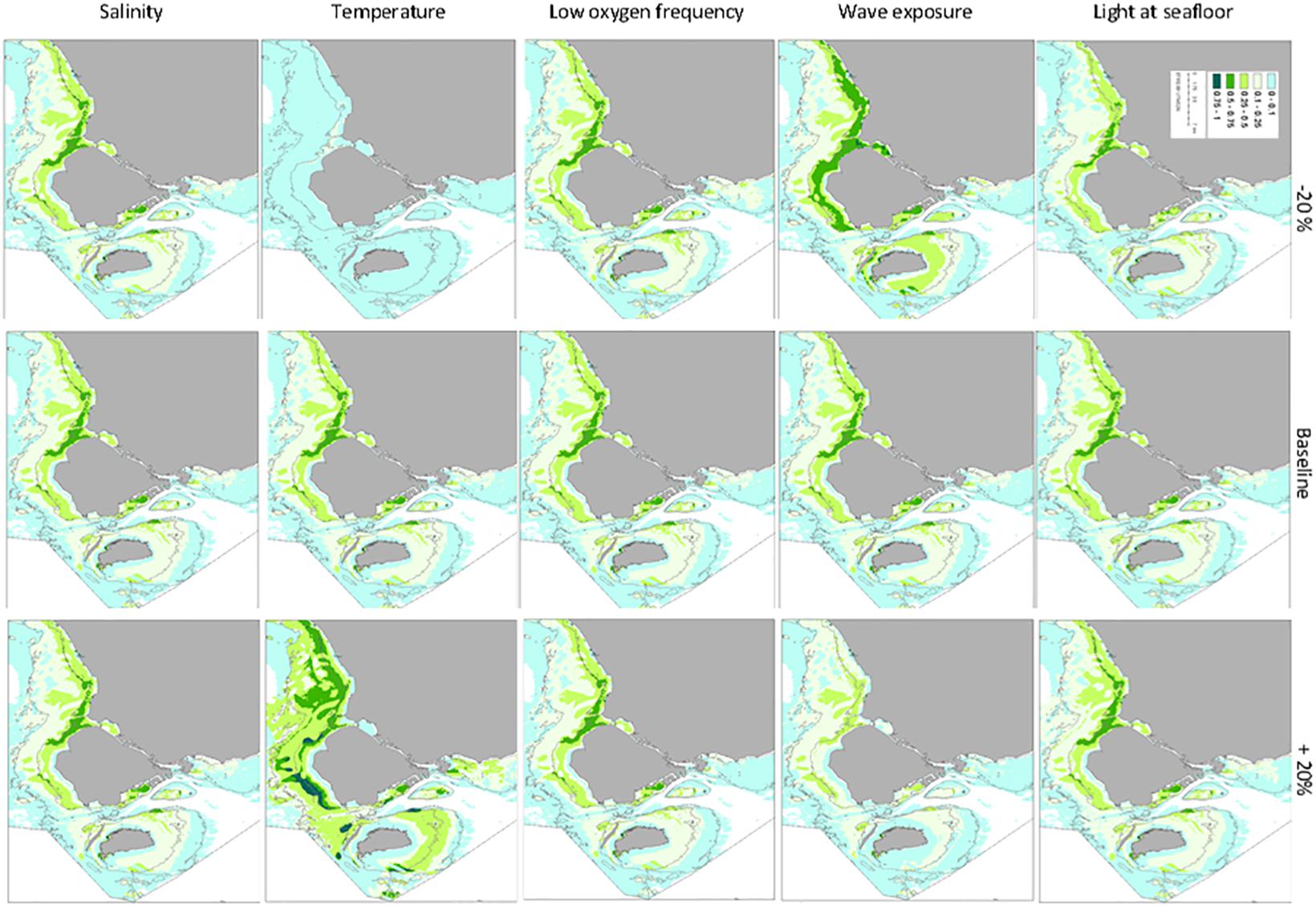
Figure 9. Sensitivity of modeled eelgrass coverage to changes in input values. The input value in each pixel was varied between -20% to +20% relative to baseline conditions.

The limitations of the current model should, however, be kept in mind. The GIS model applies data with a rather coarse resolution (100 × 100 m), implying that not all subareas are well represented by the model, simply due to absence of some of the key input data. In addition, the quality of the input data layers will largely determine the quality and predictability of the output from the GIS map. These limitations also indicate how the model can be improved in the future. Firstly, there is potential for improving the quality of the different data layers once better data are available at a national level. The physical exposure layer is an obvious candidate here. Also, as data layers representing additional potential stressors become available at a national scale, this will also help to better account for and explain local differences in regulating factors. For example, compared with local modeling in Odense fjord by Kuusemäe et al. (2016), the GIS model displays a good resemblance to scenario zero that exclude stressors such as resuspension and lugworm burial of seeds. We should also take note that the transect data, which the GIS model was fitted by, do not represent all Danish coastal waters equally. This may bias the model toward higher suitability and accuracy in areas with more observations. For example, we see that the visual fit between in situ eelgrass depth limits from 2012 and the GIS model seems better in areas with more transects and worse in areas with fewer transects. Moreover, the algorithms used to combine the GIS data layers can be improved. For example, adjustment of the applied sensitivity to water temperature could probably reduce overestimation of eelgrass presence at depth, particularly in the Kattegat region. Similarly, adjustment of the sensitivity to wave exposure could probably improve predictions in shallow waters such as Limfjorden. However, since our model aimed at a national scale, such local adjustment has not been undertaken in the current exercise. Adjustment of the individual weights of the applied indices in the combined index model could also be considered, although initial trials did not indicate improved model performance when the light and exposure indices were weighted higher. Finally, reiterating the fact that the outcome of the eelgrass model is strongly dependent on the quality of the GIS data layers used, the GIS model described here will be strengthened as new and better data layers become available. While some of these concern higher spatial resolution (e.g., sediment characteristics), others involve higher temporal resolution capable of discerning the duration of periods unfavorable (e.g., low oxygen and high temperatures) for eelgrass growth.

Conclusion

Despite limitations and precautions, the developed GIS model provides a highly useful and long-needed estimate of the current potential distribution of eelgrass in Danish waters as well as an overview of key factors regulating the national distribution of these important meadows. The model thereby constitutes a very important tool to guide the sustainable management of eelgrass meadows at a national scale.

Author Contributions

PS and KT conceived the study. PS, CG, SØ, and SU analyzed the data. PS was responsible for writing with manuscript but got considerable help from all authors.

Funding

This work was supported by the Velux Foundation through the project, Havets skove (#18530) and Storm impacts (#18538).

Conflict of Interest Statement

The authors declare that the research was conducted in the absence of any commercial or financial relationships that could be construed as a potential conflict of interest.

Supplementary Material

The Supplementary Material for this article can be found online at: https://www.frontiersin.org/articles/10.3389/fmars.2019.00175/full#supplementary-material

Footnotes

1. ^ https://oda.dk/main.aspx

References

Andersen, T., Carstensen, J., Hernandez-Garcia, E., and Duarte, C. M. (2009). Ecological thresholds and regime shifts: approaches to identification. Trends Ecol. Evol. Ecol. Evol. 24, 49–57. doi: 10.1016/j.tree.2008.07.014

PubMed Abstract | CrossRef Full Text | Google Scholar

Bekkby, T., Rinde, E., Erikstad, L., Bakkestuen, V., Longva, O., Christensen, O., et al. (2008). Spatial probability modelling of eelgrass (Zostera marina) distribution on the west coast of Norway. ICES J. Mar. Sci. 65, 1093–1101. doi: 10.1093/icesjms/fsn095

CrossRef Full Text | Google Scholar

Blok, S. E., Olesen, B., and Krause-Jensen, D. (2018). Life history events of eelgrass Zostera marina L. populations across gradients of latitude and temperature. Mar. Ecol. Prog. Ser. 590, 79–93. doi: 10.3354/meps12479

CrossRef Full Text | Google Scholar

Borum, J. (1985). Development of epiphytic communities on eelgrass (Zostera marina) along a nutrient gradient in a Danish estuary. Mar. Biol. 87, 211–218. doi: 10.1007/BF00539431

CrossRef Full Text | Google Scholar

Borum, J., Sand-Jensen, K., Binzer, T., Pedersen, O., and Greve, T. (2006). “Oxygen movent in seagrasses,” in Seagrasses: Biology, Ecology and Concervation, eds A. W. D. Larkum, R. J. Orth, and C.M. Duarte (Dordrecht: Springer),255–270.

Google Scholar

Bostrom, C., Baden, S., Bockelmann, A. C., Dromph, K., Fredriksen, S., Gustafsson, C., et al. (2014). Distribution, structure and function of Nordic eelgrass (Zostera marina) ecosystems: implications for coastal management and conservation. Aquat. Conserv. Mar. Freshw. Ecosyst. 24, 410–434. doi: 10.1002/aqc.2424

PubMed Abstract | CrossRef Full Text | Google Scholar

Brooks, R. P. (1997). Improving habitat suitability index models. Wildlife Soc. Bull. (1973-2006) 25, 163–167.

Google Scholar

Cameron, A., and Askew, N. (eds). (2011). EUSeaMap-Preparatory Action for Development and Assessment of A European Broad-Scale Seabed Habitat Map Final Report, 240. Available at: http://jncc.gov.uk/euseamap

Google Scholar

Canal-Vergés, P., Petersen, J. K., Rasmussen, E. K., Erichsen, A., and Flindt, M. R. (2016). Validating GIS tool to assess eelgrass potential recovery in the Limfjorden (Denmark). Ecol. Modell. 338, 135–148. doi: 10.1016/j.ecolmodel.2016.04.023

CrossRef Full Text | Google Scholar

Canal-Verges, P., Potthoff, M., Hansen, F. T., Holmboe, N., Rasmussen, E. K., and Flindt, M. R. (2014). Eelgrass re-establishment in shallow estuaries is affected by drifting macroalgae – Evaluated by agent-based modeling. Ecol. Modell. 272, 116–128. doi: 10.1016/j.ecolmodel.2013.09.008

CrossRef Full Text | Google Scholar

Carstensen, J., Krause-Jensen, D., Markager, S., Timmermann, K., and Windolf, J. (2013). Water clarity and eelgrass responses to nitrogen reductions in the eutrophic Skive Fjord, Denmark. Hydrobiologia 704, 293–309. doi: 10.1007/s10750-012-1266-y

CrossRef Full Text | Google Scholar

Clausen, P. (2000). Modelling water level influence on habitat choice and food availability for Zostera feeding brent geese Branta bernicla in non-tidal areas. Wildlife Biol. 6, 75–87. doi: 10.2981/wlb.2000.003

CrossRef Full Text | Google Scholar

Clausen, P., Clausen, K., Holm, T. E., and Fredshavn, J. R. (2015). Ændret Forekomst af Lysbuget Knortegås ved Mariager Fjord og Randers Fjord. Roskilde: DCE – Danish Centre for Environment and Energy, Aarhus University, 10 (in Danish).

Google Scholar

Conley, D. J., Kaas, H. M., F., Rasmussen, B., and Windolf, J. (2000). Characteristics of danish estuaries. Estuaries 23, 820–837. doi: 10.2307/1353000

CrossRef Full Text | Google Scholar

De Cock, A. (1981). Influence of temperature and variations in temperature on flowering in Zostera marina L. under laboratory conditions. Aquat. Bot. 10, 125–131. doi: 10.1016/0304-3770(81)90015-2

CrossRef Full Text | Google Scholar

Drew, E. A. (1978). Factors affecting photosynthesis and its seasonal variation in the seagrasses Cymodocea nodosa (Ucria) Aschers, and Posidonia oceanica (L.) Delile in the Mediterranean. J. Exp. Mar. Biol. Ecol. 31, 173–194. doi: 10.1016/0022-0981(78)90128-4

CrossRef Full Text | Google Scholar

Duarte, C. M., Kennedy, H., Marba, N., and Hendriks, I. (2013). Assessing the capacity of seagrass meadows for carbon burial: current limitations and future strategies. Ocean Coastal Manage. 83, 32–38. doi: 10.1016/j.ocecoaman.2011.09.001

CrossRef Full Text | Google Scholar

Duarte, C. M., and Krause-Jensen, D. (2017). Export from seagrass meadows contributes to marine carbon sequestration. Front. Mar. Sci. 4:13. doi: 10.3389/fmars.2017.00013

CrossRef Full Text | Google Scholar

Duarte, C. M., Marbà, N., Krause-Jensen, D., and Sánchez-Camacho, M. (2007). Testing the predictive power of seagrass depth limit models. Estuar. Coasts 30:652. doi: 10.1007/BF02841962

CrossRef Full Text | Google Scholar

Flindt, M. R., Rasmussen, E. K., Valdemarsen, T., Erichsen, A., Kaas, H., and Canal-Verges, P. (2016). Using a GIS-tool to evaluate potential eelgrass reestablishment in estuaries. Ecol. Modell. 338, 122–134. doi: 10.1016/j.ecolmodel.2016.07.005

CrossRef Full Text | Google Scholar

Guidance, W. C. E. (2009). Common Implementation Strategy for the Water Framework Directive (2000/60/EC). Guidance document (23). Available at: http://ec.europa.eu/environment/water/water-framework/objectives/pdf/strategy2.pdf

Google Scholar

Hemminga, M. A., and Duarte, C. M. (2000). Seagrass Ecology. Cambridge: Cambridge University Press. doi: 10.1017/CBO9780511525551

CrossRef Full Text | Google Scholar

Hilary, A. N., Frederick, T. S., Seth, B., and Blaine, S. K. (2005). Disturbance of eelgrass Zostera marina by commercial mussel Mytilus edulis harvesting in Maine: dragging impacts and habitat recovery. Mar. Ecol. Prog. Ser. 285, 57–73. doi: 10.3354/meps285057

CrossRef Full Text | Google Scholar

Hirzel, A. H., and Le Lay, G. (2008). Habitat suitability modelling and niche theory. J. Appl. Ecol. 45, 1372–1381. doi: 10.1111/j.1365-2664.2008.01524.x

CrossRef Full Text | Google Scholar

Kenworthy, W. J., Gallegos, C. L., Costello, C., Field, D., and di Carlo, G. (2014). Dependence of eelgrass (Zostera marina) light requirements on sediment organic matter in Massachusetts coastal bays: implications for remediation and restoration. Mar. Pollut. Bull. 83, 446–457. doi: 10.1016/j.marpolbul.2013.11.006

PubMed Abstract | CrossRef Full Text | Google Scholar

Koch, E. W. (2001). Beyond light: physical, geological, and geochemical parameters as possible submersed aquatic vegetation habitat requirements. Estuaries 24, 1–17. doi: 10.2307/1352808

CrossRef Full Text | Google Scholar

Krause-Jensen, D., Carstensen, J., Nielsen, S. L., Dalsgaard, T., Christensen, P. B., Fossing, H., et al. (2011). Sea bottom characteristics affect depth limits of eelgrass Zostera marina. Mar. Ecol. Prog. Ser. 425, 91–102. doi: 10.3354/meps09026

CrossRef Full Text | Google Scholar

Krause-Jensen, D., and Christensen, P. (1999). Myndighedernes kontrol-og overvågningsprogram for Øresundsforbindelsens kyst-til-kyst anlæg: Interkalibrering af havgræs (Ruppia spp.) undersøgelser 1998.

Google Scholar

Krause-Jensen, D., Markager, S., and Dalsgaard, T. (2012). Benthic and pelagic primary production in different nutrient regimes. Estuaries Coasts 35, 527–545. doi: 10.1007/s12237-011-9443-1

CrossRef Full Text | Google Scholar

Krause-Jensen, D., Pedersen, M. F., and Jensen, C. (2003). Regulation of eelgrass (Zostera marina) cover along depth gradients in Danish coastal waters. Estuaries 26, 866–877. doi: 10.1007/BF02803345

CrossRef Full Text | Google Scholar

Krause-Jensen, D., Sagert, S., Schubert, H., and Boström, C. (2008). Empirical relationships linking distribution and abundance of marine vegetation to eutrophication. Ecol. Indic. 8, 515–529. doi: 10.1016/j.ecolind.2007.06.004

CrossRef Full Text | Google Scholar

Krause-Jensen, D., Middelboe, A. L., Sand-Jensen, K., and Christensen, P. B. (2000). Eelgrass, Zostera marina, growth along depth gradients: upper boundaries of the variation as a powerful predictive tool. Oikos 91, 233–244. doi: 10.1034/j.1600-0706.2001.910204.x

CrossRef Full Text | Google Scholar

Kuusemäe, K., Rasmussen, E. K., Canal-Vergés, P., and Flindt, M. R. (2016). Modelling stressors on the eelgrass recovery process in two Danish estuaries. Ecol. Modell. 333, 11–42. doi: 10.1016/j.ecolmodel.2016.04.008

CrossRef Full Text | Google Scholar

McGlathery, K. J., Reynolds, L. K., Cole, L. W., Orth, R. J., Marion, S. R., and Schwarzschild, A. (2012). Recovery trajectories during state change from bare sediment to eelgrass dominance. Mar. Ecol. Prog. Ser. 448, 209–221. doi: 10.3354/meps09574

CrossRef Full Text | Google Scholar

Murray, C., and Markager, S. (2011). “Relationship between Secchi depth and the diffuse light attenuation coefficient in Danish estuaries,” in Proceedings of the Baltic Sea Science Conference, St. Petersburg.

Google Scholar

Nejrup, L. B., and Pedersen, M. F. (2008). Effects of salinity and water temperature on the ecological performance of Zostera marina. Aquat. Bot. 88, 239–246. doi: 10.1016/j.aquabot.2007.10.006

CrossRef Full Text | Google Scholar

Nielsen, S. L., Sand-Jensen, K., Borum, J., and Geertz-Hansen, O. (2002). Depth colonization of Eelgrass (Zostera marina) and macroalgae as determined by water transparency in Danish coastal waters. Estuaries 25, 1025–1032. doi: 10.1007/BF02691349

CrossRef Full Text | Google Scholar

Noer, H., and Petersen, B. M. (1993). Mapping of Submergent Vegetation Around Saltholm. Scientific Report. Denmark: Danmarks Miljøundersøgelser, Aarhus Universitet.

Google Scholar

O’Brien, K. R., Waycott, M., Maxwell, P., Kendrick, G. A., Udy, J. W., Ferguson, A. J. P., et al. (2017). Seagrass ecosystem trajectory depends on the relative timescales of resistance, recovery and disturbance. Mar. Pollut. Bull. 134, 166–176. doi: 10.1016/j.marpolbul.2017.09.006

PubMed Abstract | CrossRef Full Text | Google Scholar

Olesen, B., Krause-Jensen, D., and Christensen, P. B. (2017). Depth-related changes in reproductive strategy of a cold-temperate Zostera marina meadow. Estuaries Coasts 40, 553–563. doi: 10.1007/s12237-016-0155-4

CrossRef Full Text | Google Scholar

Ørberg, S. B., Groom, G. B., Kjeldgaard, A., Carstensen, J., Rasmussen, M. B., Clausen, P., et al. (2018). Kortlægning af ålegræsenge Med Ortofotos:-Muligheder og Begrænsninger. Scientific Report No. 265 (in Danish). Roskilde: DCE – National Centre for Energy and Environment, Aarhus University.

Google Scholar

Orth, R. J., Carruthers, T. J., Dennison, W. C., Duarte, C. M., Fourqurean, J. W., Heck, K. L., et al. (2006). A global crisis for seagrass ecosystems. Bioscience 56, 987–996. doi: 10.1641/0006-3568 (2006)56[987:AGCFSE]2.0.CO;2

CrossRef Full Text | Google Scholar

Phillips, R. C., Mcmillan, C., and Bridges, K. W. (1983). Phenology of eelgrass, zostera-marina l, along latitudinal gradients in North-America. Aquat. Bot. 15, 145–156. doi: 10.1016/0304-3770(83)90025-6

CrossRef Full Text | Google Scholar

Pulido, C., and Borum, J. (2010). Eelgrass (Zostera marina) tolerance to anoxia. J. Exp. Mar. Biol. Ecol. 385, 8–13. doi: 10.1016/j.jembe.2010.01.014

CrossRef Full Text | Google Scholar

Rasmussen, E. K., Petersen, O. S., Thompson, J. R., Flower, R. J., Ayache, F., Kraiem, M., et al. (2009). Model analyses of the future water quality of the eutrophicated Ghar El Melh lagoon (Northern Tunisia). Hydrobiologia 622, 173–193. doi: 10.1007/s10750-008-9681-9

CrossRef Full Text | Google Scholar

Raun, A. L., and Borum, J. (2013). Combined impact of water column oxygen and temperature on internal oxygen status and growth of Zostera marina seedlings and adult shoots. J. Exp. Mar. Biol. Ecol. 441, 16–22. doi: 10.1016/j.jembe.2013.01.014

CrossRef Full Text | Google Scholar

Riemann, B., Carstensen, J., Dahl, K., Fossing, H., Hansen, J. W., Jakobsen, H. H., et al. (2016). Recovery of danish coastal ecosystems after reductions in nutrient loading: a holistic ecosystem approach. Estuaries Coasts 39, 82–97. doi: 10.1007/s12237-015-9980-0

CrossRef Full Text | Google Scholar

Sand-Jensen, K. (1977). Effect of epiphytes on eelgrass photosynthesis. Aquat. Bot. 3, 55–63. doi: 10.1016/0304-3770(77)90004-3

CrossRef Full Text | Google Scholar

Short, F. T., Davis, R. C., Kopp, B. S., Short, C. A., and Burdick, D. M. (2002). Site-selection model for optimal transplantation of eelgrass Zostera marina in the northeastern US. Mar. Ecol. Prog. Ser. 227, 253–267. doi: 10.3354/meps227253

CrossRef Full Text | Google Scholar

Short, F. T., and Wyllie-Echeverria, S. (1996). Natural and human-induced disturbance of seagrasses. Environ. Conserv. 23, 17–27. doi: 10.1017/S0376892900038212

PubMed Abstract | CrossRef Full Text | Google Scholar

Staehr, P. A., and Borum, J. (2011). Seasonal acclimation in metabolism reduces light requirements of eelgrass (Zostera marina). J. Exp. Mar. Biol. Ecol. 407, 139–146. doi: 10.1016/j.jembe.2011.05.031

CrossRef Full Text | Google Scholar

Tallis, H. M., Ruesink, J. L., Dumbauld, B., Hacker, S., and Wisehart, L. M. (2009). Oysters and aquaculture practices affect eelgrass density and productivity in a pacific northwest estuary. J. Shellfish Res. 28, 251–261. doi: 10.2983/035.028.0207

CrossRef Full Text | Google Scholar

Valdemarsen, T., Wendelboe, K., Egelund, J. T., Kristensen, E., and Flindt, M. R. (2011). Burial of seeds and seedlings by the lugworm Arenicola marina hampers eelgrass (Zostera marina) recovery. J. Exp. Mar. Biol. Ecol. 410, 45–52. doi: 10.1016/j.jembe.2011.10.006

CrossRef Full Text | Google Scholar

Yang, S., Wheat, E. E., Horwith, M. J., and Ruesink, J. L. (2013). Relative impacts of natural stressors on life history traits underlying resilience of intertidal eelgrass (Zostera marina L.). Estuar. Coasts 36, 1006–1013. doi: 10.1007/s12237-013-9609-0

CrossRef Full Text | Google Scholar