Satellite Salinity Observing System: Recent Discoveries and the Way Forward

Introduction: Remote Sensing of Salty Oceans

Sea water is approximately a 3.5% salt solution (Durack et al., 2013; Pawlowicz et al., 2016), corresponding to a salinity of 35¹, the remaining 96.5% being freshwater. Wunsch (2015) finds the mean salinity of the entire ocean to be 34.78, with a standard deviation of only 0.37 and over 90% of sea water falling within the salinity range of 34 to 36. Despite this small range, salinity variations have a profound effect on global ocean circulation and Earth’s climate and ecosystems. Ocean basins vary in terms of their salinity (Figure 1), with the Atlantic being the saltiest ocean and the Pacific the freshest (Gordon et al., 2015). These mean patterns are a response to the changes in the ocean circulation and the ocean water cycle – the net sum of precipitation, evaporation, and terrestrial river and groundwater runoff, as well as the formation and melting of glacial and sea ice. Excess input or deficit of freshwater impacts salinity signatures, the equivalent of floods and droughts on land (Schmitt, 2008; Schanze et al., 2010; Yu, 2011; Durack, 2015; Gordon, 2016), reflecting responses to the changing hydrological cycle associated with climate change (Curry et al., 2003; Boyer et al., 2005; Hosoda et al., 2009; Durack and Wijffels, 2010; Helm et al., 2010; Durack et al., 2012; Skliris et al., 2014; Vinogradova and Ponte, 2017).

FIGURE 1

Figure 1. Example of synoptic, near-global salinity coverage from satellite observations showing annual mean sea surface salinity patterns based on observations from the Aquarius mission during 2011–2014. Credit: NASA.

As might be expected, the ocean hydrological cycle has the greatest impact on the ocean surface layer, but this signal, governed by ocean dynamics, runs deep and varies greatly across the ocean regimes as the surface water spreads into the full volume of the ocean through vertical and horizontal (or isopycnal and diapycnal) advective and diffusive processes (Ponte and Vinogradova, 2016).

Ocean salinity is not a passive tracer of ocean dynamics as salinity, along with temperature and pressure, is a component of the equation of state of sea water. Increased salinity increases density, unless offset by an increase in temperature. The ratio of the salinity to temperature impact on density changes with temperature, with salinity taking on a larger role in cold polar waters because the coefficient of thermal expansion diminishes as the temperature drops and the haline contraction coefficient increases with cooler temperatures. As salinity alters the density field, it influences horizontal pressure gradients of the flow as well as the vertical stability of the water column. Such changes, in turn, affect ocean currents and mixing, influencing the transport of oceanic properties such as heat, freshwater, nutrients, and carbon. Given its critical role in ocean dynamics, climate variability, the water cycle, and marine biogeochemistry, salinity is recognized as an essential climate variable within the Global Climate Observing System (GCOS) (Belward et al., 2016).

Observing salinity from space offers the advantages of global coverage and the ability to capture space and time scales not afforded by in situ platforms such as vessels, moorings, and Argo profiling floats. For example, the nominal sampling of the Argo array is one profile per 3° latitude × 3° longitude at 10-day intervals. There are generally very few Argo floats in marginal seas, coastal oceans, polar oceans, and in regions of large-scale divergence, where salinity variations have strong impacts on ocean dynamics, air-sea and ocean–ice interactions, and land-sea linkages (Figure 2). Salinity remote sensing complements the in situ salinity observing system by improving the capability to study mesoscale salinity variability (see sections “Improving Knowledge of Ocean Circulation and Climate Variability” and “Complementing the in situ Salinity Network”) and land-sea linkages in the context of the water cycle and biogeochemical cycles (more in section “Opening the Window to Better Understand Earth’s Water Cycle”).

FIGURE 2

Figure 2. Variability in space-borne sea surface salinity during 1 year (colors) superimposed with locations of currently operational Argo floats (white dots). Notice that regions of high variability of >0.2 are either not sampled or poorly sampled by Argo, including coastal oceans, western boundary currents, the Indonesian Seas, outlets of major rivers (Amazon, Niger, and Congo), as well as the Southern and Arctic Oceans.

In the latter third of the 20th century, an impressive array of ocean information was derived remotely from orbiting satellites, but only in the 21st century have we gained satellite views of sea surface salinity (SSS). Satellite measurements have given us a near-global, synoptic view of SSS (e.g., Figure 2), opening a window to a fuller understanding of the global hydrological cycle, climate variability, ocean circulation, and marine biochemistry. The satellite missions pioneering salinity remote sensing include the ESA Soil Moisture and Ocean Salinity (SMOS) Mission (2009-present) (Reul et al., 2012); the joint NASA/CONAE Aquarius/SAC-D mission (June 2011–June 2015) (Lagerloef et al., 2013); and the NASA Soil Moisture Active Passive (SMAP) mission (January 2015-present) (Entekhabi et al., 2014; Tang et al., 2017).

All three satellite SSS missions provide measurements of the surface brightness temperature at L-band radiometric frequencies (∼1.4 GHz), a frequency band in which brightness temperature has good sensitivity to SSS in warm (>5°C) waters (Klein and Swift, 1977). Aquarius and SMAP have similar active-passive designs, with an active L-band radar scatterometer integrated with the passive L-band radiometer. SMOS is solely based on passive L-band interferometric radiometry. For all three missions, the process of retrieving SSS from brightness temperatures involves removing various, non-salinity contributions related to direct and ocean-reflected extra-terrestrial radiations from the Sun and galaxy (e.g., Le Vine et al., 2005; Reul et al., 2007, 2008), as well the noise from sea surface temperature (SST) and ocean surface roughness (e.g., Yueh et al., 2010, 2013, 2014; Meissner et al., 2014, 2018). The latter is one of the dominant errors sources in the SSS retrieval budget that must be precisely removed. While the L-band radar on Aquarius was used to correct for the surface roughness effect, SMAP’s active radar ended operation 3 months after launch. Consequently, the correction of the surface roughness effect in both SMOS and SMAP SSS retrievals rely on ancillary wind data and on roughness information inferred from polarized L-band brightness temperature. For SSS retrievals, all three L-band missions use ancillary SST measurements to remove thermal effects on brightness temperature measurements. The adequacy and accuracy of ancillary wind and SST measurements are very important to the uncertainties of SSS retrievals.

All three SSS-observing satellites are in sun-synchronous polar orbits with high inclinations, allowing near-global coverage including the polar oceans. The missions differ in their spatial and temporal coverage. SMOS has an average 43-km spatial resolution with an 18-day near-repeat cycle and a 3–5 day revisit time. Aquarius had a 100–150 km spatial resolution and a 7-day exact repeat. SMAP has a 40-km spatial resolution and an 8-day repeat with a 2–3 day revisit time. Therefore, all three missions provide synoptic measurements of SSS over the global ocean at spatial and temporal scales much finer than those afforded by the Argo array; consequently, satellite SSS measurements are able to resolve higher-frequency signals (e.g., tropical instability waves) that are difficult for in situ data to capture.

Satellite SSS measurements serve a broad user community from scientific research to applications. These include studies of ocean dynamics, the ocean’s role in climate variability, linkages with the hydrological and biogeochemical cycles, ocean state estimation, ocean forecasts and climate predictions, and environmental assessments associated with extreme events such as hurricanes and flooding. The science and application drivers of satellite SSS in support of these user communities are discussed in Sections “Scientific Drivers for Satellite Salinity” and “Application Drivers for Satellite Salinity.”

The objective of this review is to provide community inputs to OceanObs’19 on the issues related to the space-based salinity observing system. In what follows, we (1) summarize the achievements and current capabilities of the satellite SSS observing system; (2) describe science and application drivers, user communities of satellite SSS for the coming decade, and their associated requirements; (3) address the necessity and benefits of integrating satellite SSS with other observing systems and models; and (4) discuss the strategy that addresses capability gaps in the coming decade to improve support of end users.

Scientific Drivers for Satellite Salinity

Improving Knowledge of Ocean Circulation and Climate Variability

Salinity remote sensing has significantly improved our ability to study large-scale ocean processes. Examples include the studies that brought new knowledge about tropical instability waves (Lee et al., 2012, 2014; Yin et al., 2014), Rossby waves (e.g., Menezes et al., 2014; Banks et al., 2016), dynamics of the subtropical salinity maximum and tropical salinity minimum zones (e.g., Hasson et al., 2013; Bingham et al., 2014; Hernandez et al., 2014; Yu, 2014; Gordon et al., 2015; Guimbard et al., 2017; Hasson et al., 2018), and climate variability (Delcroix, 1998; Delcroix et al., 2007; Du and Zhang, 2015; Vinogradova and Ponte, 2017). These studies are among many other that have demonstrated that the space-time resolution and coverage of salinity satellites provide a unique perspective, enhance the ocean observing network, and complement in situ salinity observations.

For example, one of the early scientific results based on satellite SSS is the discovery of new features of tropical instability waves. Tropical instability waves play an important role in ocean mixing, cross-equatorial transport, climate variability, and biochemistry, and have been studied extensively using various satellite and in situ observations since they were discovered in the late 1970s (e.g., Legeckis, 1977; Chelton et al., 2000). Complementing previous studies, satellite SSS observations revealed previously unreported features of tropical instabilities waves, including the dependence of the wave propagation speed on latitude and the phase of the El Niño-Southern Oscillation (ENSO) (Lee et al., 2012; Yin et al., 2014). The findings provided new insights into the inter-hemispheric exchange of freshwater, with implications on ocean circulation and the hydrological cycle (Lee et al., 2012).

The high temporal resolution of satellite SSS enabled a better understanding of large-scale intra-seasonal phenomena (e.g., Subrahmanyam et al., 2018), including the Madden-Julian Oscillation (MJO) – the dominant climate mode at sub-seasonal time scales in the tropics that impacts the global weather and climate (Zhang, 2005). Satellite SSS measurements enable characterization of the SSS signature associated with MJO and the associated impacts on surface density variations (Grunseich et al., 2013; Guan et al., 2014; Li et al., 2015), emphasizing the role of upper-ocean dynamics in regulating MJO.

Satellite salinity has also improved our understanding of seasonal-to-interannual variability. For example, satellite SSS measurements revealed new features of annual Rossby waves in the South Indian Ocean associated with coupled air-sea and surface–subsurface interactions (Menezes et al., 2014). On interannual time scales, satellite SSS measurements demonstrated their value in helping to characterize the structure of the Indian Ocean Dipole (IOD) (Durand et al., 2013; Du and Zhang, 2015), which is known to influence regional weather and climate (Saji et al., 1999). The superior spatio-temporal sampling of satellite SSS helped establish a robust relationship between SSS and the IOD (Du and Zhang, 2015). Another example of new insight enabled by satellite SSS is the relationship between the large-scale tropical fresh pools in the tropical Pacific with ENSO-induced precipitation and oceanic transport associated with mesoscale eddies (Alory et al., 2012; Guimbard et al., 2017; Hasson et al., 2018; Figure 3). The two examples of the linkages of SSS with climate modes (ENSO and the IOD) demonstrate the potential of satellite SSS to improve the representation of climate variability in ocean models and related forecasts, e.g., through SSS data assimilation.

FIGURE 3

Figure 3. Satellite SSS are used to monitor large-scale events, including ENSO-induced fresh anomalies that are propagated by mesoscale processes. Shown here are time-longitude plots of SMOS SSS, averaged between (left) 2°S and 2°N and (right) 16°N and 20°N. NINO3.4 index is shown on top of all plots, blue during La Nina and red during El Nino. For the first time, strong negative salinity anomalies that stretch over the tropical Pacific and reach the Hawaii islands have been detected, induced by an extreme El Nino event of October 2015–2016. Modified from Hasson et al. (2018).

Decadal changes in salinity serve as an important indicator of the internal climate fluctuations (as opposed to externally caused variability due to anthropogenic and natural forces), and help explain longer-term secular changes in the climate system (e.g., Friedman et al., 2017). Informed by satellite salinity data through data assimilation and synthesis with other ocean observations and dynamical constraints, Vinogradova and Ponte (2017) reported significant large-scale SSS trends as yet more evidence of global climate change. Some portion of the decadal fluctuations in surface salinity, however, is associated with natural climate variability, such as the Interdecadal Pacific Oscillations (IPO, Figure 4), which effectively masks long-term salinity trends that are related to secular changes in the forcing.

FIGURE 4

Figure 4. Surface SSS trends as indicator of internal climate variability. Tropical changes in SSS over the past 20 years are partly attributed to Interdecadal Pacific Oscillation (IPO), explaining strong surface salinification in the Pacific warm Pool (red) despite an increase of flux of freshwater into the ocean (blue in Figure 5). Based on multi-platform salinity estimate ECCO that combines satellite and in situ data with dynamical constraints. Shown here are (A) Expression of the IPO loading pattern in surface salinity, computed by linearly regressing monthly ECCO salinity anomalies upon (B) the IPO time series in normalized units of standard deviation. (C) Trends in the IPO loading salinity patterns. (D) Residual trends after the relevant IPO loading pattern is removed. Trends in panels (C,D) represent the total change over 20 years, computed as a linear trend multiplied by the period length. Adapted from Vinogradova and Ponte (2017). Figure^© Copyright July 2017 AMS.

Opening the Window to Better Understand Earth’s Water Cycle

Over the global ocean, the most significant moisture sources are located in the subtropical oceans (e.g., Figure 5), where the descending branch of Hadley circulation suppresses convection and precipitation, while prevailing trade winds promote evaporation (Gimeno et al., 2012). To maintain the global water balance (Schmitt, 1995; Trenberth and Guillemot, 1995; Stohl and James, 2005; Trenberth et al., 2007), this excessive flux of moisture from the ocean to the atmosphere is transported away from the subtropics to the tropical oceans over the ITCZ (Inter Tropical Convergence Zone), the mid-latitude storm-track region, and over land as terrestrial precipitation (Gimeno et al., 2010; Lagerloef et al., 2010; Schanze et al., 2010; van der Ent et al., 2010).

FIGURE 5

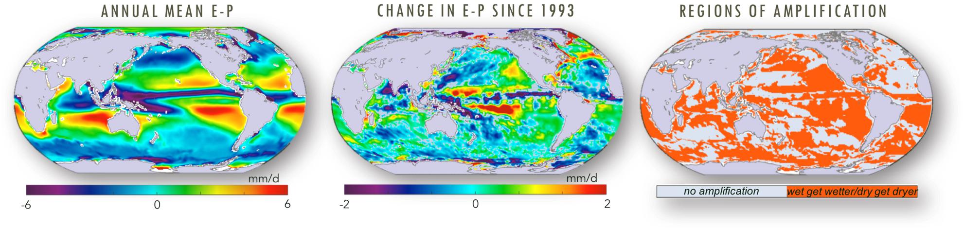
Figure 5. Linking salinity to the global hydrological cycle is one of scientific drivers of satellite SSS. Shown here are mean patterns of the ocean water cycle and its amplification in the last two decades based on the ECCO ocean state estimate. Left: average rates at which freshwater enters (blue) or leaves (red) the ocean via the processes of precipitation (P) and evaporation (E); Middle: trends in E-P; blue (negative) means that the ocean received more freshwater since 1993. Right: Amplification of the ocean water cycle, computed as a slope of the linear regression between the anomalies and trends in E-P. Pattern amplification is shown as orange, otherwise is shaded gray. In many ocean regions, pattern amplification follows the wet gets wetter/dry gets drier paradigm, as more freshwater is brought to wet regions (e.g., blue colors match blue in the tropics), or more freshwater is removed from dry regions (e.g., red colors match red in the United States west coast. If averaged over the globe, the ocean water cycle has amplified by 5% since 1993. See Vinogradova and Ponte (2017) for details.

Observational and modeling evidence suggests that in response to the warming climate, surface freshwater fluxes over the oceans have developed a distinctive pattern of change (Figure 5), where dry subtropical areas are becoming drier and wet tropical areas becoming wetter (Stott et al., 2008; Cravatte et al., 2009; Durack and Wijffels, 2010; Helm et al., 2010; Durack et al., 2012; Terray et al., 2012; Skliris et al., 2014, 2016; Vinogradova and Ponte, 2017; Zika et al., 2018). For example, from the ECCO state estimate and Figure 5, over the past two decades the ocean water cycle amplified by about 5% on average, consistent with surface warming of about 0.65°C since 1992. That translates to a change of 7.6%°C^-1, which is close to that predicted by the thermodynamics and the Clausius–Clapeyron relation of 7%°C^-1. This intensification of the hydrological cycle is often linked to corresponding changes in surface salinity: the changes in the amount of freshwater leaving and entering the oceans are expected to leave its “fingerprints” detectable in ocean variables, with SSS variability reflecting the changes in the ocean water cycle (Schmitt, 2008; Durack and Wijffels, 2010; Lagerloef et al., 2010; Yu, 2011; Durack et al., 2012; Terray et al., 2012; Durack, 2015; Friedman et al., 2017). Although a direct link between changes in surface salinity and changes in freshwater flux is rather difficult to observe on timescales relevant to the satellite observational records (Vinogradova and Ponte, 2013a, 2017; Hasson et al., 2014; Yu, 2015; Guimbard et al., 2017), the research community consensus, outlined in Durack et al. (2016), is that ocean salinity can be effectively used as an implicit, rather than explicit, indicator of changes in the water cycle.

An important application of satellite salinity is connecting the terrestrial and marine water reservoirs, with an aim to close the global balance of water fluxes and flows. Combined with other measurements, satellite SSS observations allow one to trace large riverine waters over great distances and reconstruct the complete lifecycle of hydrological events, from rainfall to river discharge on land and then to river plume formation, mixing, and advection in the ocean (Fournier et al., 2011; Bai et al., 2013; Gierach et al., 2013; Reul et al., 2013; Grodsky et al., 2014; Guerrero et al., 2014; Zeng et al., 2014; Fournier et al., 2015, 2016, 2017a,b; Korosov et al., 2015). These studies improved our understanding of ocean–land interactions by elucidating the impacts of rivers on the buoyancy of the surface ocean layer, on circulation patterns via horizontal density gradients, on marine biochemistry, the carbon cycle, and on ecological activity (Muller-Karger et al., 1988; McKee et al., 2004). In addition to tracing the origin and fate of freshwater signals, satellite SSS has also been used to gauge the influence of rivers on regional climate and oceanic productivity (Fournier et al., 2017a), as well as the impacts of the river-influenced warming on the upper ocean during the Atlantic hurricane season (Fournier et al., 2017b).

New Opportunities in Mesoscale Oceanography

A tremendous advantage of satellite SSS observations is their synoptic view of oceanic mesoscale haline features associated with fronts and eddies down to scales on the order of 100 km (e.g., Maes et al., 2014; Reul et al., 2014a; Kolodziejczyk et al., 2015; Fournier et al., 2016, 2017b; Isern-Fontanet et al., 2016; Da-Allada et al., 2017; Grodsky et al., 2017; Melnichenko et al., 2017). The capability to systematically sample 40–100 km scales every 4 days is unachievable by other salinity observing platforms, including the Argo program. Although smaller eddies are still difficult to detect by the current generation of salinity-measuring satellites, the capability to monitor salinity features associated with the larger eddies is a breakthrough both in terms of spatial and temporal sampling. As an illustration, Figure 6 compares complex current and frontal systems depicted by satellite SSS with those inferred from Argo. Mesoscale fronts are important components of ocean dynamics because they are associated with strong current instability and ocean mixing. Oceanic fronts have enhanced vertical velocity, where the deep ocean exchanges properties with the surface mixed layer (Pollard and Regier, 1992). Enhanced vertical nutrient fluxes at fronts act to increase phytoplankton production and biomass, funneling nutrients through different trophic levels, including to commercially important fish (Woodson and Litvin, 2015).

FIGURE 6

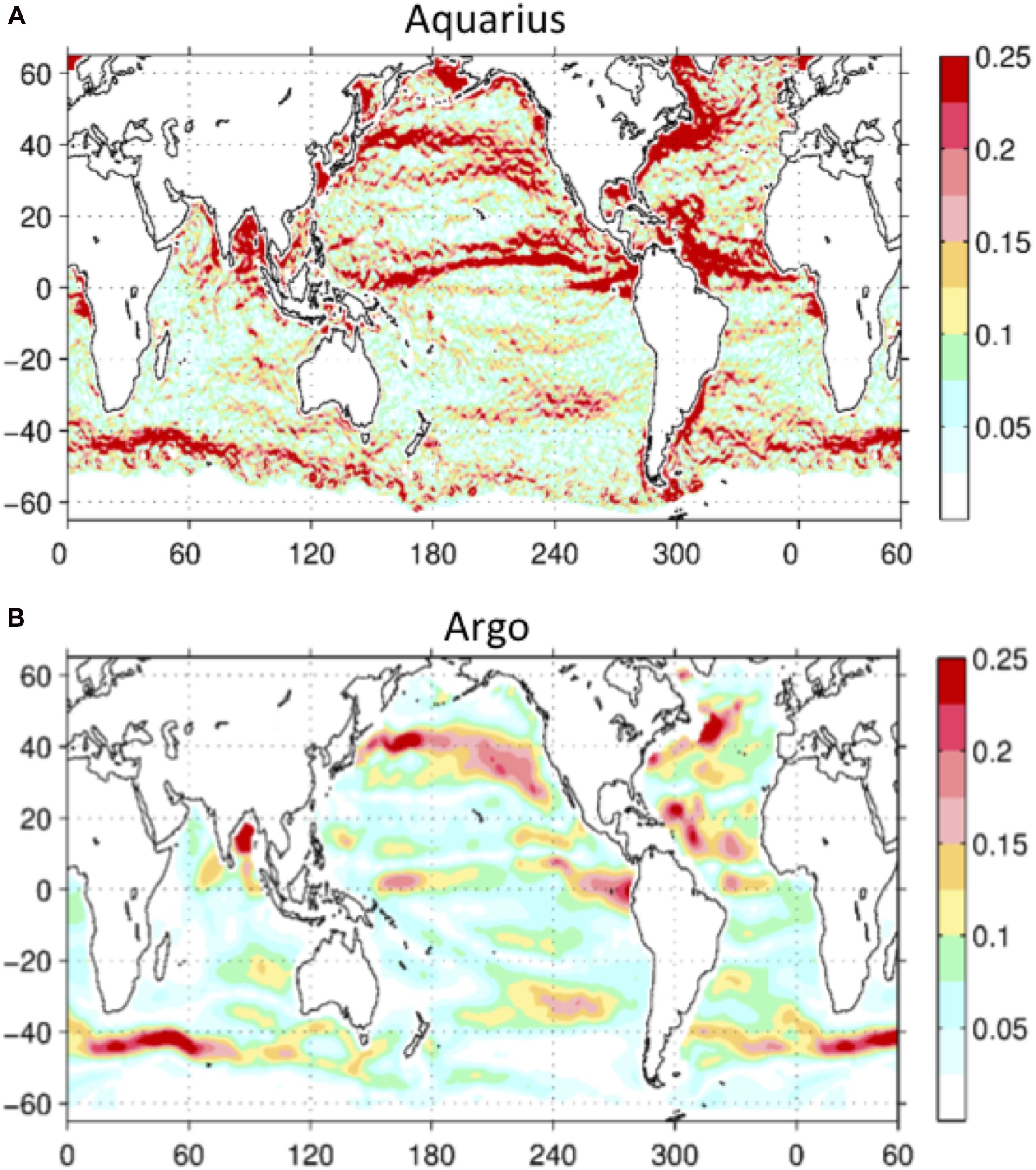
Figure 6. Salinity SSS resolve fine mesoscale features, such as fronts and eddies, that are not depicted by blurry maps computed based in situ-based products; (A) Map of the horizontal SSS gradient magnitude (pss/100 km) based on the September 2011 mean SSS field from the Aquarius satellite. The oceanic frontal zones are associated with high values of SSS gradient (red). (B) The same as in panel (A) but from the Argo-derived SSS. Modified from Melnichenko et al. (2016).

While satellite SST observations have long been available to study oceanic fronts and eddies, satellite SSS observations bring a new perspective. By discovering SST/SSS decoupling in the frontal regions (Kolodziejczyk et al., 2015; Kao and Lagerloef, 2018), we are redefining the role of salinity in density variability, thermohaline circulation, and in the energy balance of the upper ocean. Satellite SSS observations also improved the ability to study the kinetic energy variability of ocean circulation (Gordon and Giulivi, 2014; Reul et al., 2014a; Sommer et al., 2015; Busecke et al., 2017; Melnichenko et al., 2017), elevating the role of eddy transport in the ocean freshwater balance, even in the interiors of the subtropical gyres where eddies have historically been thought to have a negligible effect.

Unlocking Space-Based Ocean Biogeochemistry

Expanding upon the conventional physical oceanography boundaries, satellite SSS data has been recently exploited in the biogeochemistry domain (e.g., Lee et al., 2006; Lefèvre et al., 2014; Ibánhez et al., 2017), addressing studies of ocean acidification and the carbon cycle. Since the industrial revolution, the oceans have absorbed about 40–50% of the anthropogenic carbon dioxide (CO₂) emissions to the atmosphere (Sabine et al., 2004; Khatiwala et al., 2009), mitigating the impact of global warming. However, studies have suggested that the oceanic carbon sink may have been decreasing during the last 50 years (Canadell et al., 2007; Le Quere et al., 2009), which can significantly impact future atmospheric CO₂ levels and the global climate.

Absorption of CO₂ into the ocean reduces the ocean pH and the concentration of carbonate ions. The overall process is referred to as ocean acidification, which has profound socio-economic consequences. In order to characterize the overall marine carbonate system, the partial pressure of CO2 in surface seawater (pCO₂), the total alkalinity, the dissolved inorganic carbon, and the pH itself must be known. However, the difficulty in quantifying these parameters is due to the scarcity of biochemical in situ observations, such as the SOCAT dataset (Bakker et al., 2016). In this regard, satellite SSS data (together with additional observables) offers a path forward to monitor ongoing changes in ocean acidification by exploiting synoptic satellite observations to produce global assessments of ocean surface pH and alkalinity (Brown et al., 2015; Land et al., 2015; Sabia et al., 2015a; Salisbury et al., 2015; Fine et al., 2017).

Similar to salinity, alkalinity is sensitive to freshwater flux. Consequently, alkalinity features resemble the mean surface salinity distribution (Figure 7), with salinity variations explaining 80% of total alkalinity variability in the subtropics. That makes salinity a valuable proxy for surface alkalinity. Taking advantage of global, high-resolution satellite SSS measurements, it is now possible to derive space-based assessments of ocean acidification and observe how it changes over time (Fine et al., 2017). The results suggest a tendency of generally increasing alkalinity in the subtropics (along with increasing temperature and salinity), reinforcing the assessment of ocean acidification from uptake of atmospheric CO₂.

FIGURE 7

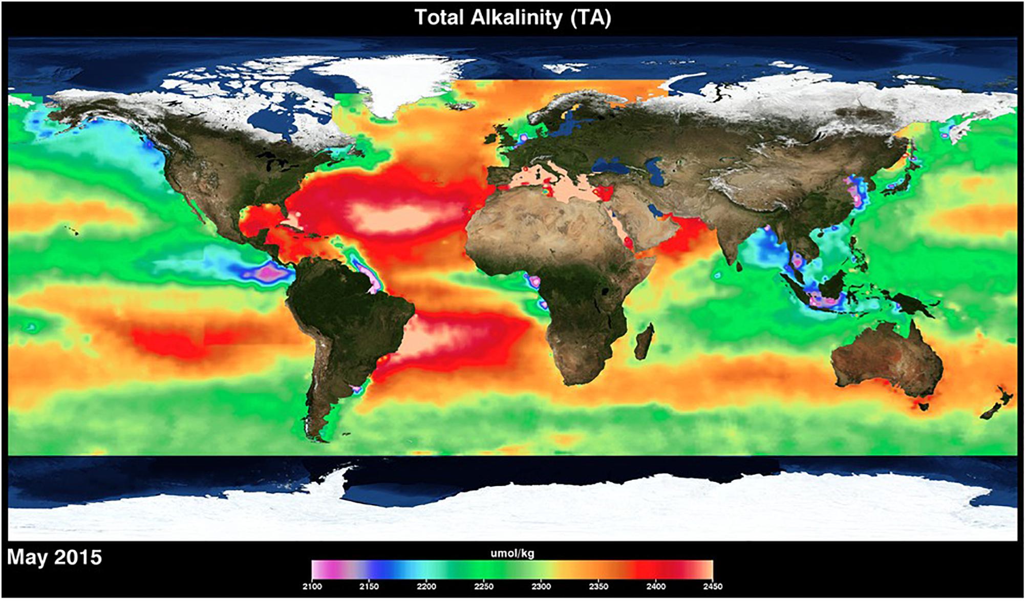
Figure 7. Satellite SSS data becoming key in monitoring the marine carbonate system, enabling the development of novel space-based ocean acidification. Shown here is monthly surface total alkalinity derived using Aquarius SSS. Source: NASA.

Advancing Climate Modeling and Ocean State Estimation

A powerful approach in modern oceanography is to combine observations and models – be they ocean-only or fully coupled simulations – using various data assimilation techniques. More than a decade of experience with assimilating in situ salinity data from surface moorings and three-dimensional measurements from Argo, ships, etc., has demonstrated that the resulting synthesis product can provide a more accurate estimate of the ocean state than observations or model alone (Stammer et al., 2002a,b, 2016; Wunsch and Heimbach, 2013), including better handling of climate simulations of air-sea coupling and resulting changes in ocean circulation. By observing the top centimeter of the water column globally, dense satellite SSS data provides additional constraints on interfacial exchanges of water between the atmosphere and the upper-ocean, helping close the global freshwater budget, improve estimates of the ocean state, and inform future climate projections. If performed in a dynamically consistent way, the data assimilation process will not only improve the model’s salinity fields and derivatives such as circulation fields and sea level, but will also help better constrain the mean and time-varying surface net freshwater forcing and air-sea fluxes (Stammer et al., 2004; Carton et al., 2018), which are some of the least constrained parameters in climate models leading to large uncertainties in model simulations.

Assimilation of satellite SSS data helped improve the accuracy of model salinity and air-sea fluxes within the Estimating the Circulation and Climate of the Ocean (ECCO) solution (Köhl et al., 2014). By providing additional constraints on model freshwater fluxes, the assimilation of satellite SSS reduced uncertainties in surface forcing, producing a better correspondence between models and independent satellite-based air-sea fluxes, and reduced known model salinity biases with respect to in situ measurements.

Today, the ECCO framework reconciles various salinity observations from different platforms (as well as observations for other state variables) using dynamical constraints, and produces an accurate, multi-platform salinity estimate for climate research (Figure 8; see also Vinogradova et al., 2014; Fukumori et al., 2018; Vinogradova, 2018). Such a synergistic, dynamically consistent view becomes an additional component of the salinity observing network – a component allowing one to tease out the causes and effects of recent salinity changes from the interplay between the three-dimensional ocean circulation, transports of salt and freshwater, and surface forcing.

FIGURE 8

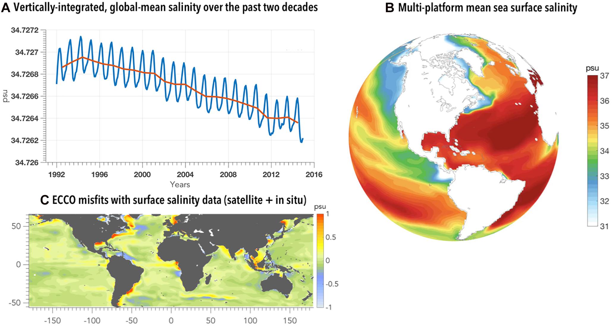
Figure 8. Information from satellite SSS data improves climate models and ocean state estimates in systems like ECCO. (A) Vertically integrated, globally averaged salinity over the past two decades computed from monthly (blue) and annual (red) values. The global mean salinity value is 34.72, with a narrow range over the oceans. Notice a global freshening trend, with a drop of about –0.0005 pss/20 years, which represents the net transfer of mass into the ocean due to freshwater exchange. The value is consistent with the global-mean mass variations observed by GRACE, equivalent to –0.0004 pss/20 years. (B) Annual mean patterns in surface salinity from ECCO, featuring salty subtropics and fresher tropical and high-latitude regions, a generally saltier Atlantic and a fresher Pacific ocean. (C) ECCO/data misfits at the model surface (satellite and in situ), with distribution close to Gaussian (not shown). In most ocean regions, the misfits are less or around 0.1 of the observed averaged (green), apart from several coastal regions with higher systematic biases. Adapted from Vinogradova (2018).

Application Drivers for Satellite Salinity

In addition to science priorities, there is a wide range of emerging societal applications and end users of salinity remote sensing data, including hurricane monitoring; prediction of rain, floods, and droughts; understanding climate modes of variability; and improving ocean and ecological forecasting.

Hurricane Monitoring

In monitoring hurricanes, it is sea surface temperature and sea surface height that first come to mind as measures of ocean heat content available for storm formation and intensification. However, in recent years, there has been growing interest in the role and response of SSS in hurricane intensification and passage. In regions where salinity is an important driver of vertical stratification, such as tropical oceans near the outflows of major rivers, SSS can impact air–sea interactions. In these regions, low SSS helps the formation and maintenance of a thin surface mixed layer, along with an isothermal salinity-stratified “barrier” layer between the surface mixed layer and colder thermocline water (Lukas and Lindstrom, 1991; Pailler et al., 1999; Vinaychandran et al., 2002; Rao and Sivakumar, 2003; Balaguru et al., 2012, 2015, 2016).

On one hand, the barrier layer helps trap solar radiation in the surface layer (Ffield, 2007; Foltz and McPhaden, 2008; Vizy and Cook, 2010; Grodsky et al., 2012; Fournier et al., 2017a), leading to elevated SSTs that are favorable for deep atmospheric convection and strong rainfall (Shenoi et al., 2002). On the other hand, barrier layers can prevent vertical mixing and entrainment of cool thermocline water into the mixed layer (Vialard and Delecluse, 1998; Vincent et al., 2012; Thadathil et al., 2016), thus further supporting hurricane intensification (Cione and Uhlhorn, 2003; Sengupta et al., 2008; Balaguru et al., 2012; Grodsky et al., 2012; Neetu et al., 2012; Reul et al., 2014b).

Satellite SSS measurements are able to capture haline wakes that form after hurricane passage, particularly in regions where upper-ocean stratification is driven by salinity (Figure 9). By analyzing hundreds of storms in the Atlantic Ocean, recent studies (Grodsky et al., 2012; Reul et al., 2014b; Fournier et al., 2017a) demonstrate the effect of barrier layers on hurricane intensification, emphasizing the role of salinity stratification in mixed-layer dynamics and the use of satellite SSS data as a new resource to study the ocean response to tropical cyclones.

FIGURE 9

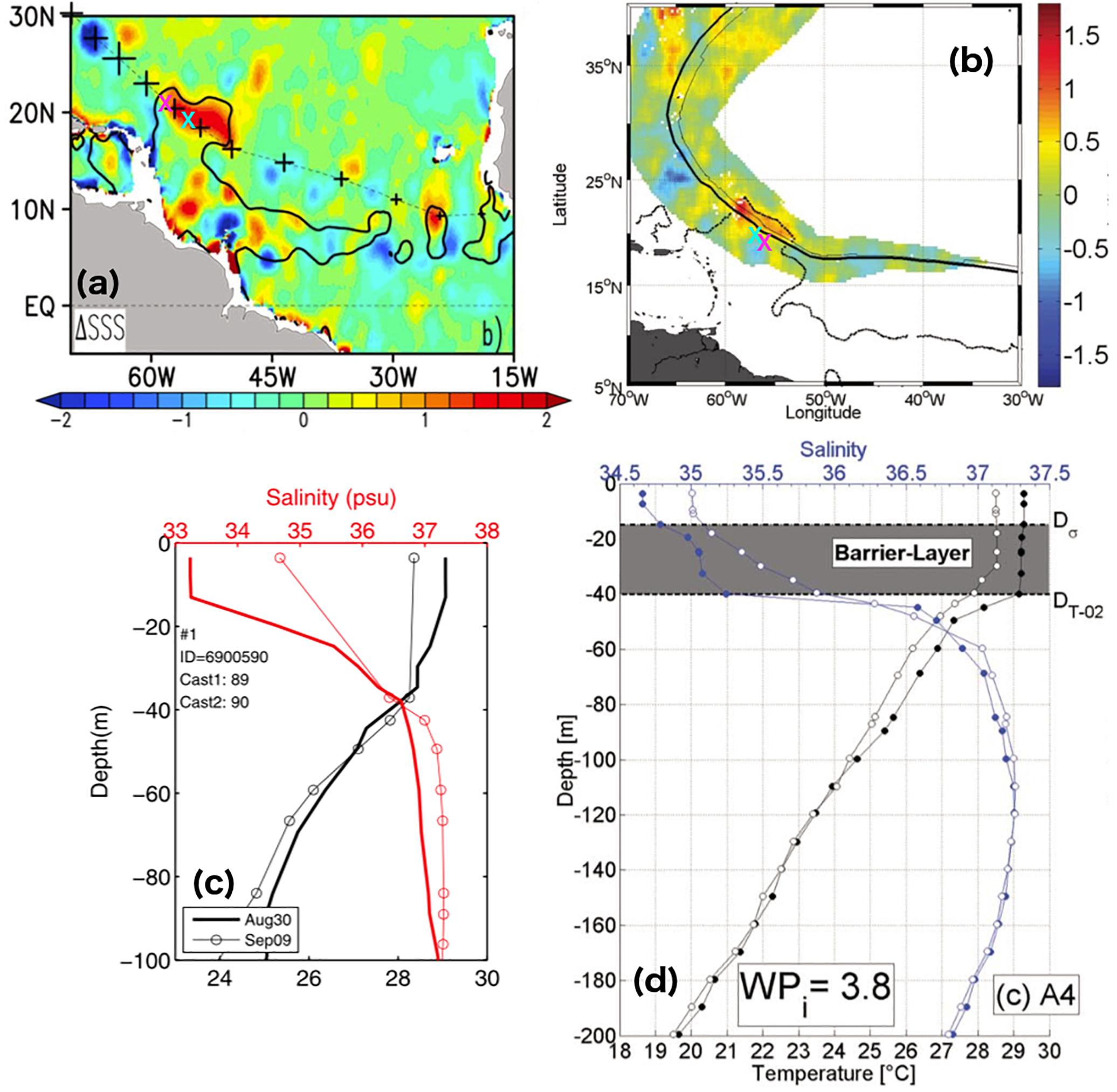
Figure 9. Monitoring hurricanes using satellite SSS data from panel (a) Aquarius and (b) SMOS, respectively, showing differences from after versus before Katia and Igor hurricane passages in the Atlantic Ocean. (c,d) Argo salinity profiles before and after the hurricanes passage. The location of the Argo floats are marked by magenta and cyan crosses in panels (a,b). Figure sources: Grodsky et al. (2012) and Reul et al. (2014b). Reproduced under license agreement 4445231502401 and 4445231097796.

Toward Better ENSO Forecasting

The ENSO cycle with alternating El Niño and La Niña events is the dominant year-to-year climate signal on Earth. ENSO originates in the tropical Pacific through interactions between the ocean and the atmosphere, but its environmental and socioeconomic impacts are felt worldwide, ranging from agriculture, to marine ecosystems, to human health (Horel and Wallace, 1981; Glantz, 2001). Efforts to understand the causes and consequences of ENSO reveal the breadth of ENSO’s influence on the Earth system and the potential to exploit its predictability for societal benefit (McPhaden et al., 2006; National Academies of Sciences, Engineering, and Medicine, 2016).

One key component of ENSO predictability is the impact of freshwater flux in the tropics on coupled modeling. Representation of tropical precipitation, including the double-ITCZ biases (e.g., Adam et al., 2018), is rather poor in the current generation of coupled models (Wang et al., 2010), with implications for coupled forecast results. Systematic misrepresentation of precipitation results in erroneous surface forcing, impacting the correctness of the initialization and forecasting of ocean salinity. Inaccurate salinity, in turn, leads to the misrepresentation of mixed-layer density, barrier-layer thickness, and upwelling in the ocean model, as well as subsequent ramifications for ENSO predictions from the coupled model.

Recent studies demonstrate that using salinity observations is a promising tool for understanding and expanding the limits of ENSO prediction (Maes et al., 2005; Hackert et al., 2011, 2014; Zhu et al., 2014). In practice, accounting for the salinity structure provides better estimates of the barrier layer thickness and mixed-layer dynamics, including the increase in stability of the mixed layer that allows the wind forcing to be more efficient. The latter, in particular, enhances the ocean’s sensitivity to Kelvin wave forcing, resulting in the overall improvement of coupled ENSO predictions.

Predicting Terrestrial Floods and Droughts

Oceans are the major suppliers of moisture to land and significantly impact terrestrial precipitation, including hydroclimate extremes such as floods, droughts, and water shortage (Gimeno et al., 2013).

Given the limited water-holding capacity of the land surface, intense and persistent precipitation events cannot be sustained by local moisture recycling (Brubaker et al., 1993; Trenberth, 1998, 1999; Koster et al., 2004; Dirmeyer et al., 2009) and for the majority of extreme rainfall events over land, the moisture supply has oceanic origins (Zhou and Yu, 2005; Weaver and Nigam, 2008; Chan and Misra, 2010; Cook et al., 2011; Kunkel et al., 2012; Li et al., 2013). Correspondingly, any deficit in oceanic moisture supply usually leads to drought and water shortage (Weaver et al., 2009a,b; Seager and Vecchi, 2010). Thus, the oceanic water cycle, by modulating the regional moisture balance, significantly affects hydroclimate extremes on land.

The close linkage between the oceanic and terrestrial components of the Earth’s water cycle, along with the sensitivity of SSS to the oceanic component, suggests that SSS can be utilized as a predictor of precipitation on land. Recent evidence has shown how salinity information can add great value to the early-warning systems of hydrology-related natural disasters. In particular, the linkage between the oceanic water cycle, soil moisture content, and local land-atmosphere interaction (Figure 10) suggests that pre-season SSS is a physically meaningful predictor of the summer precipitation in the United States Midwest (Li et al., 2016a), winter precipitation in the southwestern United States (Liu et al., 2018), and monsoonal precipitation in the African Sahel (Li et al., 2016b). These studies found that SSS ranked as the most important predictor of land precipitation in those regions compared to ten other climate indices, including SST. We note that this linkage between terrestrial rainfall and subtropical SSS via the atmospheric moisture transport is another aspect of the land-sea linkages that is different from the direct land-sea linkage through river discharge as discussed in Section “Opening the Window to Better Understand Earth’s Water Cycle.”

FIGURE 10

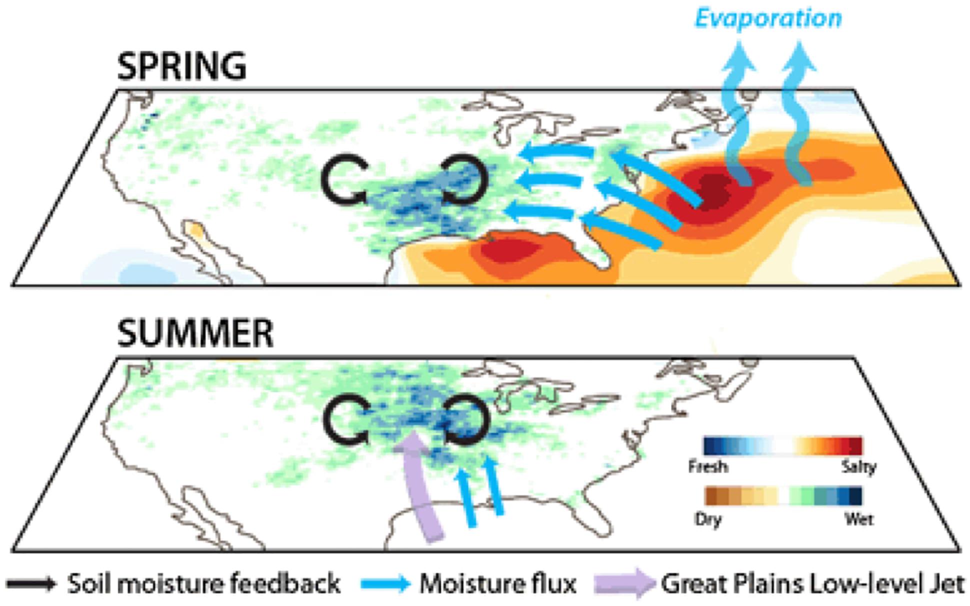
Figure 10. Satellite SSS data improves prediction of land precipitation. Schematic figure illustrating the soil moisture mechanism bridging the 3-month time lag between springtime salinity anomalies and summer precipitation in the United States Midwest: in the western North Atlantic, higher springtime salinities are an indicator of enhanced moisture export onto the continental United States which converges in the South. This greatly increases soil moisture there, allowing for enhanced evaporation and leading to more atmospheric convection on land (upper panel). The intensified convection on land draws in more moisture from the Gulf of Mexico and leads to the enhancement of the Great Plains Low Level Jet, which carries moisture to the upper Midwest in summer (bottom panel). Adapted from Li et al. (2018), reproduced under Creative Commons license.

Inferring Rainfall Over the Oceans

While more than 75% of precipitation occurs over the ocean, using satellite salinity as a direct rain gauge has proven challenging because both freshwater fluxes and ocean dynamics govern SSS variability (e.g., Vinogradova and Ponte, 2013a, 2017; Hasson et al., 2014; Yu, 2015; Guimbard et al., 2017). However, the window of opportunity may lie within a very short time period (typically 30 min) in tropical ocean regions where SSS freshening is strongly correlated with instantaneous rain rates similar in magnitude to those expected from earlier conceptual modeling studies (Boutin et al., 2016).

Despite recent advances, measurements of rain rate suffer from significant uncertainties and discrepancies, particularly within the ITCZ regions (Liu and Zipser, 2014). To reduce uncertainty, information on rain rate derived from satellite SSS sensors could provide an independent constraint over the ocean, where very few in situ rain rate measurements exist. Improving information on rain rates inferred from satellite L-band radiometry has two main challenges. One is related to difficulties in modeling the processes controlling the rain penetration into the upper ocean, keeping in mind that L-band radiometer signals penetrate only the upper few cm of the surface. Another challenge is constraining the physics of L-band radiometer measurements under rain conditions, including the characterization of the rain-induced surface roughness (e.g., Tang et al., 2013). In addition, reconciling point in situ observations or one-dimensional models with satellite observations needs to take into account the spatial heterogeneity of rain and SSS within a satellite pixel. The latter need could be addressed by taking advantage of the combination of multi-satellite information, such as SMOS and SMAP crossing points that are less than one hour apart (Supply et al., 2017), as well as measurements from synthetic aperture radar (SAR), rain radar, and other global precipitation mission (GPM) radiometers for characterizing the variability of rainfall, which is very intermittent.

Ocean Forecasting on the Horizon

Operational ocean forecasting systems, including those contributing to GODAE OceanView (Le Traon et al., 2015), assimilate ocean observations into high-resolution ocean models. Reanalyses and real-time forecasts produced by these systems are used to generate information about the past, current, and future ocean state, which is provided to downstream users. The quality of the information provided is dependent on the model and observations, and on the data assimilation system used to combine them. Unlike climate models, operational systems run close to real time, and thus the input streams need to be robust and timely, as well as be of good quality with known accuracy. To meet this need, sequential data assimilation (e.g., Carton et al., 2018) offers an alternative to the costly adjoint computations of climate-oriented ocean state estimates, ensuring computational efficiency of the operational ocean estimates and forecasts.

Although, at the moment, no ocean forecasting systems assimilate satellite SSS data operationally, there have been a number of efforts to develop schemes to do so by investigating the SSS data’s impact on the ocean analyses and forecast. For example, as part of the ESA SMOS-NINO15 project, Martin et al. (2018) show how assimilation of satellite SSS data into the Met Office Forecasting Ocean Assimilation Model (FOAM) had a positive impact on the forecasting of tropical salinity changes, with an overall reduction in the root-mean-square (RMS) difference to Argo near-surface salinity data by 8%. These improvements in near-surface salinity also led to improvements in other modeled variables, including sea surface temperature and sea level. Positive impacts (a 5% RMS difference reduction) were also found in the Mercator-Ocean analysis and forecasting system, which was used to carry out a similar experiment during the 2015 ENSO event.

Another contributor to the GODAE OceanView program that aims to exploit satellite SSS data is NOAA’s Real-Time Ocean Forecast System (RTOFS) for global and regional (United States west coast) applications. The project is at an early stage, with data streams from SMOS and SMAP incorporated into NOAA’s environmental modeling data tank for model initialization and future assimilation. Ongoing test studies are encouraging, demonstrating improved representations of extremes of simulated sea-surface height anomalies, ocean surface density, mesoscale dynamics, and upper-ocean heat content), as well as better salinity constraints for downscaling to nested regional ocean/coastal models (Boukabara et al., 2016).

While recent results demonstrate the potential for operational assimilation of satellite SSS data (Toyoda et al., 2015), a number of issues need to be addressed prior to it becoming a reality. The bias correction of the satellite data relies on good quality in situ reference data, so improving the coverage of in situ SSS data should be a priority, especially in marginal seas, coastal regions, and high-latitude oceans. The timeliness (latency) of the data streams also needs to improve so that data are available for use within 24 h of measurement time, with the delivery of near real-time data being robust. Continuing improvement in the quality of the SSS retrievals and error/uncertainty information provided with the data will also feed into improved assimilation results.

Opportunity for Integration

As a newcomer, salinity remote sensing seamlessly integrated into the broader salinity network and global Earth observing system. Having global coverage with more uniform and finer spatio-temporal sampling, satellite SSS data complements sparser in situ salinity observations, filling in sampling gaps for regions with few in situ measurements such as in river plumes, coastal oceans, and marginal seas (Figure 2). Exploring how satellite SSS observations fit into a broad observing system in more detail, the following thoughts suggest a path for making satellite SSS data integration more meaningful.

Complementing the in situ Salinity Network

Ship observations, as well as measurements from drifters and moorings, tend to have high temporal resolution and accuracybut limited spatial coverage. Thus, satellite SSS measurements are useful for placing in situ observations in a broader context. Satellite SSS measurements are often used to interpret in situ observations during field experiments (e.g., Mahadevan et al., 2016), as well as to verify the presence of various ocean features that have large spatial scales, such as river plumes (Grodsky et al., 2014), eddies (Reul et al., 2014a), and ENSO signatures (Hasson et al., 2014).

In general, salinity data from satellite and Argo profiling floats are highly complementary: gridded satellite data have spatial resolutions as fine as a few tens of km on approximately weekly intervals, while the Argo array has a nominal sampling of one float per 3°×3° at 10-day intervals. Thus, combining the two datasets improves detection and characterization of mesoscale features, such as fronts and eddies that are not well captured by Argo alone (e.g., Grodsky et al., 2012; Reul et al., 2014a; Grodsky and Carton, 2018; Kao and Lagerloef, 2018) while mitigating the large-scale biases of satellite SSS. These synergistic products show particular improvement of salinity variability in regions where Argo floats are sparse (Toyoda et al., 2015; Lu et al., 2016) or regions with high variability such as that caused by ocean currents (Chakraborty et al., 2015). Moreover, satellite SSS alleviate the sparse sampling of in situ measurements in coastal oceans and marginal seas, thereby enhancing the capability to study land-sea linkages.

Prominent examples of the successful synergy between the satellite and in situ salinity observations are the NASA field campaigns Salinity Processes in the Upper-Ocean Regional Study, experiments 1 and 2, or SPURS-1 and SPURS-2, respectively (Lindstrom et al., 2015; SPURS-2 Planning Group, 2015). The SPURS program seeks better understanding of the global freshwater cycle through investigation of all the physical processes controlling the upper-ocean salinity balance. Set in ocean regions with evaporating (SPURS-1) and precipitating (SPURS-2) regimes, SPURS involves coordinated field work using moorings, autonomous instruments, ship-based process studies, remote sensing, and modeling. By combining large-scale Argo arrays with synoptic satellite images and local measurements from moorings, drifters, gliders, and microstructure profiling, the SPURS framework allows salinity variability to be observed across a range of scales, placing local and high-resolution salinity signals into a broader, mesoscale and basin-wide context.

Synergies With Other Satellite Measurements

In addition to complementing the in situ salinity network, satellite SSS has become an integral part of the globalspace-based Earth observing system, further enhancing a synergistic use of multi-variable satellite observations to address various Earth system science questions and applications.

Combined use of satellite SSS with other satellite measurements has enabled an array of new discoveries and capabilities, examples of which were highlighted above. Blended satellite and in-situ SSS (e.g., Melnichenko et al., 2014) enhanced the salinity monitoring capability. In particular, NOAA’s Blended Analysis of Surface Salinity (Xie et al., 2014) based on Aquarius, SMOS, SMAP, and in situ salinities are produced operationally and used for monthly global ocean monitoring. Satellite SSS and SST together have made it possible to estimate surface density from space, facilitating the study of the surface water-mass formation processes (Sabia et al., 2015b) and linkages between the atmosphere and the deeper ocean. Combining SSS with altimetric measurements of sea surface height has allowed the quantification of eddy energy balance and to identify new features in mesoscale and large-scale oceanography. Combining satellite SSS, ocean currents, and precipitation has provided a powerful tool to study the effect of ocean circulation in mediating the ongoing changes in the hydrological cycle. The combined use of satellite SSS, soil moisture, precipitation, and ocean color data has helped identify the influence of riverine waters on ocean circulation.

Synthesis of satellite SSS and other ocean observations (both satellite and in situ) using ocean general circulation models in systems like ECCO help constrain the relatively uncertain estimates of freshwater exchange across the air-sea interface and produce multi-platform salinity estimates for climate research. As coupled assimilation capabilities advance in the coming decade, the value of satellite SSS to constrain air-sea and land-sea freshwater fluxes in coupled models will become even greater.

Complimentary by nature, physical-biogeochemical coupling provides another niche for satellite SSS integration opportunities. All carbon-related algorithms require contemporaneous information on SSS, SST, ocean color, and winds in order to estimate air-sea CO₂ flux, highlighting the need of satellite SSS in researching Earth’s carbon. Promising results of such synergies were reported as part of the Pathfinders Ocean Acidification project and call for sustained and increasing research efforts in space-based biochemistry. In this regard, the ESA project OceanSODA aims to develop novel algorithms to advance the synergistic exploitation of satellite data for producing carbonate system parameters and to assess the potential impacts of these products on science, applications, and society.

Improving the Satellite SSS Error Budget for More Meaningful Integration

Reconciling and integrating information from various sources requires careful consideration of data uncertainties and errors. Traditionally, evaluation of satellite SSS data is performed through comparisons with in situ near-surface salinity measurements from ground-truth targets collected by Voluntary Observing Ships, Argo floats, tropical moorings, and ship-based CTD or thermosalinograph (TSG) measurements, as well as with gridded maps based on these in situ salinity measurements (Drucker and Riser, 2014; Tang et al., 2014, 2017; Boutin et al., 2016, 2018; Lee, 2016). Comparison against this ground-truth data provides a measure of satellite data biases and uncertainties.

In general, the differences between two salinity estimates from various sources (e.g., satellite vs. in situ) are attributed to two types of errors: observational errors and sampling errors. Sampling errors arise when one data type does not represent a process (or scale) that the other does², e.g., due to the differences in their spatial and/or temporal samplings. Sampling errors are the “expected” differences, the low bound at which two estimates are allowed to differ, and should not be confused with measurement errors. Thus, to interpret and understand the differences between datasets, it is crucial to separate those error sources. This is particularly important to assess whether a satellite dataset meets the mission accuracy requirement, by taking into account the sampling differences from in situ measurements that are considered ground truth.

Typically, observational errors for calibrated in situ salinity data are very small, on the order of ±0.01 (e.g., Delcroix et al., 2005). For satellite SSS, observational errors are much larger primarily due to the relatively low signal to noise ratio, and to inaccuracies in satellite data calibration and SSS retrievals, ranging from imprecise modeling of the surface roughness impact, galactic radiation scattered by the sea surface, contamination by signals from land, rainfall, sea ice, sun, and radio frequency interference (RF), cold water sensitivities, and inaccuracies of ancillary data used in retrievals such as wind and SST (Le Vine et al., 2005, 2007; Font et al., 2010). For comparison, the accuracy for monthly satellite SSS at 100 × 100 km² is between 0.13 and 0.20, on average (Lagerloef et al., 2015; Tang et al., 2017; Boutin et al., 2018; Kao and Lagerloef, 2018).

Unlike the observational errors, sampling errors are couple-dependent (i.e., dependent on the two measurements being compared), and what is noise for one couple can be a non-issue for another. For example, satellite SSS retrievals represent the Gaussian-weighted average within the satellite footprint (40 km for SMOS and SMAP, and 150 km for Aquarius). In contrast, in situ measurements are pointwise observations. Thus, variability within a satellite pixel is smoothed in the satellite footprint, giving rise to a sampling error when compared with a point measurement (Figure 11). Sampling noise associated with sub-footprint variability can be a significant source of errors for in situ measurements in regions with strong transient dynamics, such as tropical regions influenced by rain bands, or regions affected by meandering currents and river plumes (Vinogradova and Ponte, 2013b; Boutin et al., 2016). While an issue in satellite/in situ comparisons, small-scale error is not a concern for comparing satellite and climate models with similar horizontal resolutions of ∼1°. A potential concern for model/satellite comparisons is temporal aliasing of the satellite monthly fields (Vinogradova and Ponte, 2012). Models generally have high temporal resolution (an hour or less) and hence produce robust monthly mean average fields, unlike satellite SSS retrievals that have 3 to 7-day sampling intervals that can introduce aliasing errors when representing the true monthly averages (Figure 11).

FIGURE 11

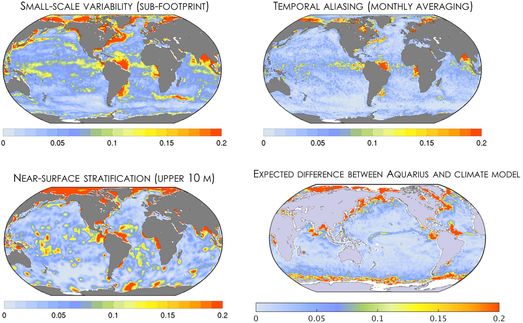
Figure 11. Example of potential sampling errors associated with small-scale (sub-footprint) variability, temporal aliasing of satellite monthly fields, and salinity near-surface stratification in the upper ten meters. Total expected difference (as data error variance, in units pss²) for the Aquarius SSS and a climate model. While small in the open ocean, sampling errors can be large in coastal regions and should be taken into account (removed) when estimating pure observational error for satellite salinity, as well as when reconciling (assimilating) it with other information. For example, such a correction can reach 0.7 pss near the Amazon, 0.5 pss in the Gulf Stream, and 0.4 pss in the Bay of Bengal. For details, see Vinogradova and Ponte (2012, 2013b) and Vinogradova et al. (2014).

With a few exceptions, both in situ and model pairings with satellite SSS will likely have representation errors associated with the sampling depth. While L-band satellites measure salinity in the top few cm of the ocean, the shallowest measurement depths for in situ sensors are typically 2 to 5 m (for most Argo floats) and 1 m for tropical moorings. Recent measurements of near-surface salinity structure show that there are situations where salinity stratification exists above 1 m, especially in the tropics where the effect of transient rain is important (Boutin et al., 2016; Drushka et al., 2016). The effect of near-surface stratification is summarized in a community paper by Boutin et al. (2016), providing the first step toward creating a systematic process of satellite SSS validation and performance assessments.

Until recently, sampling errors arising from sub-footprint variability, smoothing, and unresolved vertical gradients were not taken into account as they were assumed to be an order of magnitude smaller than the noise in satellite SSS. However, this is not the case in areas of high salinity variability. In order to improve the assessment of satellite SSS data and its integration with in situ measurements, it is necessary to better characterize the spatio-temporal distribution and decorrelation scales of the SSS variability at various scales. As an illustration, Figure 11 shows the possible amplitudes of the known sources of sampling error for satellite, in situ, and model SSS estimates. These uncertainties are typically small in the open ocean, but could be significant regionally, particularly near the outflows of major rivers, western boundary currents, etc., and can reach one in extreme cases. If trying to estimate pure observational error for the satellite SSS retrievals by comparing it with in situ measurements, these sampling errors should be taken into account (removed). If the RMS difference between the satellite and in situ data is a measure of satellite SSS error, all sampling errors should be subtracted from the total RMS in a root-sum-square sense (assuming that all contributions are uncorrelated). While relatively small in the open ocean, such corrections can be significant. For example, using the values from Vinogradova and Ponte (2012, 2013b) and Vinogradova et al. (2014) and Figure 11, the sampling error correction can reach 0.7 in the vicinity of the Amazon river, 0.5 along the Gulf Stream, and 0.4 in the Bay of Bengal, indicating the importance of taking into account the sampling errors of pointwise in situ measurements in evaluating the uncertainties of satellite SSS.

In addition to comparing satellite SSS with in situ data and estimates from climate models, satellite-to-satellite comparisons open another route for evaluating data performance. Outside of the aforementioned regions with high sampling noise, the agreement between the satellite SSS data from different missions is remarkable (Boutin et al., 2018), allowing potential errors in in situ measurements to be identified (Tang et al., 2017). To facilitate this a potential way forward is to develop a common validation framework for multiple salinity satellites. Such a framework could include data from all L-band salinity satellites (SMOS, SMAP, and Aquarius), additional related datasets (precipitation, evaporation, and SST), databases of in situ salinity measurements for match-ups (Argo, TSG, moorings, and drifters), and inter-comparison reports at different spatio-temporal scales. On the horizon, ESA’s Pilot Mission Exploitation Platform for Salinity project (Pi-MEP) aims to implement such a framework for SMOS salinity data. Similar efforts for SMAP and Aquarius in a potential partnership between ESA and NASA are under discussion.

Finally, another way to have more meaningful estimates of the satellite SSS error budget is to define appropriate metrics and indicators of data performance. The most commonly used quality indicators are the bias, the standard deviation, and the RMS differences between satellite and in situ salinities. These indicators enable a broad assessment of improvements or degradations of different versions of satellite products, provided that the reference in situ measurements and the spatio-temporal smoothing applied to the satellite measurements are the same. However, the details in how the data are processed and compared can affect the comparisons. For example, stringent filtering and data smoothing can potentially result in a very good standard deviation and RMS difference, while discarding the outliers that contain the true natural variability. Examples include eddies in river plumes (Akhil et al., 2016), small-scale salinity gradients relevant for advection studies (Hoareau et al., 2018), and others. Moving forward, it is desirable to expand the list of quality indicators that can provide information on the regional signal-to-noise ratios and the scales of variability detectable by satellite SSS measurements. For example, comparison of statistical distributions of SSS, could be effective for detecting outliers and quantifying extreme events (Supply et al., 2017; Olmedo et al., 2018), assuming sampling errors are properly addressed.

Complementary to the empirical approach to estimating the accuracy of satellite SSS, estimates of retrieval errors for satellite SSS from Aquarius have also been made available to users. The retrieval errors include the uncertainties related to factors such as instrument noise, ancillary data product uncertainties (e.g., wind and SST data to correct for surface roughness effect and thermal effects on brightness temperature measurements; Lagerloef et al., 2015), contamination near land and sea ice, and lack of sensitivity to salinity signals in cold waters (<5C, e.g., Meissner et al., 2018). Effort is also underway to obtain similar retrieval error estimates for SMAP SSS.

Looking Ahead

Although progress in the satellite salinity observing system is commendable, its continued existence, maintenance, and innovation cannot be taken for granted. Drawing on the previous sections, we summarize the need for system continuity and enhancement, suggesting potential strategies for the upcoming decade and identifying potential stakeholders that could benefit from the uniqueness of satellite salinity products.

The Need for Continuity

Many of the science and application drivers discussed in Sections “Scientific Drivers for Satellite Salinity” and “Application Drivers for Satellite Salinity” require the continuity of satellite SSS. A longer record of satellite SSS will greatly benefit the understanding and prediction of interannual climate variability, including ENSO. In order to improve the robustness of a model’s forecast skills, records of multiple realizations of interannual events are required, given the diversity of events such as the various flavors of ENSO.

Satellite SSS continuity is necessary to support longer-term monitoring and forecasting of synoptic extreme events, such as hurricanes and flooding. We have just scratched the surface of the ocean’s salinity role in hurricanes, potentially bringing new approaches into the mix of tools necessary for tropical cyclone monitoring and forecasting. A way forward in hurricane forecasting is through improving the representation and coupling of physics in the underlying atmospheric and ocean models. Satellite SSS data, with its unique very-near surface as well as synoptic coverage, is key to understanding the exchange of heat across the air-sea boundary that fuels hurricane formation and evolution, particularly in regions that are influenced by strong freshwater input. Terrestrial floods, as another type of extreme event that impacts marine ecosystems, infrastructure, and economy, will also benefit from the continuity of satellite SSS data. This is especially the case because the continuity of satellite SSS is pivotal to monitoring the impacts of the changing water cycle on land-sea linkages. Newly developed techniques for monitoring and predicting extreme events using salinity are promising, but require continued measurements in order to be statistically robust.

Increasing statistical robustness through a longer satellite SSS record is also required to confirm new discoveries in mesoscale oceanography enabled by salinity remote sensing. A large and growing body of evidence suggests that temporal variability in eddy freshwater transports is particularly important and can be related to large-scale climate forcing. This interplay between scales is, however, poorly understood. Continuing satellite SSS observations at mesoscale resolution to accumulate a longer observational record is therefore critical to understanding these processes and scale interactions.

For operational oceanography, such as ocean and ecological forecasts, continuity of satellite SSS is key. There is little incentive from operational centers to exploit observations within an operational modeling framework without a sustained measurement system.

Moving toward decadal and longer observational coverage will clarify the role of salinity in the broader climate system and its linkages with the Earth hydrological and carbon cycles. As an interwoven component of ocean circulation and stratification, ocean biochemistry, and the global water budget, salinity is an important link connecting Earth’s fundamental cycles. As the Earth’s systems are undergoing dramatic transformations, long-term salinity trends will be another independent indicator of the Earth’s health, now and in the future. Sustaining an accurate global satellite salinity observing system will make connecting the dots a reality. SSS is an essential climate and ocean variable of the GCOS. Recognizing the importance and advantages of satellite SSS, the 2016 GCOS Implementation Plan specifically recommended “Action 032: Ensure the continuity of space-based SSS measurements” (Belward et al., 2016).

The Need for Enhancement

Although it has been demonstrated that satellite SSS measurements improve many areas of science and applications much improvement in salinity remote sensing is still needed. The community recommends potential enhancements in three areas: accuracy, resolution, and coverage of satellite SSS.

Accuracy – Reducing Uncertainties

Despite their profound impact, salinity variations are rather subtle. Long-term trends in salinity are particularly subdued, ranging by 0.2 over multiple decades. In order to detect variations in salinity with high fidelity, including those variations associated with long-term climate changes, the accuracy of satellite SSS retrievals needs to be improved.

Similarly, accuracy must be improved to better resolve other ocean features of small magnitude, including eddies. With a typical eddy signal in SSS of 0.1–0.5 and an RMS error of satellite retrievals of a similar scale, the signal-to-noise ratio at mesoscale time and space scales is low. Therefore, to enhance the stability of the satellite SSS observing system SSS accuracy of less than 0.1 would be desirable. To achieve this goal, improvements in both retrieval algorithms and sensor technology are needed.

There is a sense of urgency to monitor high-latitude regions, making it imperative that salinity remote sensing reduces large uncertainties from satellite SSS data in cold waters, where retrievals are affected by reduced sensitivity of L-band brightness temperature and sea ice contamination. The unprecedented changes in sea ice melt, precipitation, and river runoff in the Arctic Ocean impact both geophysical and biochemical systems, including freshwater storage and export, ocean–ice–atmospheric interactions, primary production, and the ocean’s response to acidification. Enhancing the accuracy of satellite SSS data over the Arctic will allow systematic monitoring of the changing Arctic SSS patterns and tracking of the pathways of freshwater as it enters the North Atlantic Ocean. Similar issues arise with large uncertainties of cold Antarctic waters, affecting our ability to accurately document the variability of the Subantarctic Front and Polar Front zones, along with the related water-mass formation processes that affect global overturning rates. To monitor the ongoing changes in the polar oceans, technology development that addresses the current capability gap in a cost-effective way is necessary.

Resolution – Monitoring Mesoscale Features

While current satellite missions have substantially advanced our understanding of variations in SSS, a significant part of the ocean variability associated with mesoscale and submesoscale processes is still missing. In practice, resolving ocean features requires capturing the scale of the so-called Rossby radius of deformation – a length scale at which ocean currents feel the effects of the Earth’s rotation. In the ocean, the Rossby radius varies geographically, ranging from 200 km near the equator to 10–20 km in high latitudes (Chelton et al., 1998). The SSS measurements from the currently operating satellite missions SMOS and SMAP have spatial resolutions of approximately 40 km, which means that they only resolve the Rossby radius (and ocean eddies) up to 30° away from the equator. Therefore, it is advantageous to increase the spatial resolution of satellite SSS to better resolve mesoscale variability and to measure closer to the coasts to further enhance the studies of land-sea linkages.

Recent studies elevated the role of ocean submesoscale currents O(1–10 km), demonstrating their key contribution to the Earth energy budget and marine biogeochemistry (e.g., Su et al., 2018). However, measuring submesoscale SSS from space is beyond the current capability of L-band satellite remote sensing. Significant technology innovation is underway with the SMOS High Resolution (SMOS-HR) concept currently studied at CNES that can potentially provide 10-km resolution data during the coming decade.

Coverage – Better Sampling of Coastal Oceans

Better satellite coverage is needed near the continental margins, including near major river plumes that have implications for hydrological cycle closure. Although current salinity missions provide SSS data as close as 40 km to the coast, land contamination remains a concern, with uncertainties exceeding 1 within 100 km distance from the coast. With growing scientific and public interest in SSS data near the coasts, it is becoming critical to resolve coastal processes, including land-sea exchange, hydrological and biochemical cycles, coastal upwelling, freshening, pollution, and other processes that impact biology, the ecosystem, and human health.

Overall Strategy for Next Decade

Because salinity is an essential ocean and climate variable, the future of salinity observations impacts the success of the Global Ocean Observing System, including the network of Earth observing satellites. Given the network’s integrated nature, future satellite SSS missions will benefit from a synergistic approach to the observing system that will target critical components of the Earth system, including ocean circulation, air-sea exchanges, the hydrological cycle, and biogeochemistry. The longevity of the satellite SSS observing network relies on both technological developments and strong partnerships, driven by the common goal of advancing science and applications for societal benefit.

Strategy for Technological Innovations – Simultaneous Measurements by Multiband Radiometers

The science and application drivers, together with the challenges ahead, set specific requirements for the coming decades for satellite SSS in order to better support end-users. With a synergistic observing system in mind, one requirement is to monitor SSS at 25-km spatial resolution or less, which is the resolution of current SST and wind measurements made by passive microwave radiometers, and with global coverage at least every 3 days. Coincident measurements of SST and wind greatly facilitate SSS retrieval because, as Section “Introduction: Remote Sensing of Salty Oceans” notes, SST and wind are needed as ancillary data in SSS retrievals. The possibility of simultaneous measurements of SSS, SST, and winds is especially relevant for the tropical, low-latitude regions, where existing satellite SSS measurements are most accurate. The concept of multifrequency radiometers is being explored, specifically those covering a combination of P-, L-, C-, and/or X-bands. As all geophysical parameters can be measured at multiple microwave frequency bands, multiband microwave radiometers will be able to combine data retrieved from several bands in order to achieve improved and simultaneous measurements.

In order to enable remote sensing of SSS in cold water around the polar regions, concepts involving P-band radiometers are being considered. It has been recognized since the 1970s that the optimal radio frequency for salinity remote sensing is between 500 and 800 MHz (Wood et al., 1975; Swift and Mcintosh, 1983; Kendall et al., 1985). At these frequencies, the sensitivity to salinity is nearly invariant with water temperature and is up to 3 times more sensitive than at L-band for water temperatures less than 10°C. However, the first missions were formulated with radiometers that operated in the protected Earth Exploration Satellite Service (EESS) spectrum from 1.4 to 1.427 GHz for passive radiometry use due to concerns of radio-frequency interference (RFI) (Kerr et al., 2001; Lagerloef et al., 2008; Entekhabi et al., 2010; Oliva et al., 2016). Recently, microwave radiometer technology has evolved to filter RFI and extract clean signals if present, expanding the potential spectrum of operation (Ruf et al., 2006; Misra et al., 2013, 2018; Piepmeier et al., 2014). Radiometers with the ability to measure the spectrum in the range of 0.8–3 GHz can give the same benefit of simultaneous wind and SST retrieval, and significantly improve salinity measurements in general and in cold water in particular.

Such a system would also have applications for the cryosphere and the polar oceans (Lee et al., 2016). Current radar measurements of sea ice thickness have relatively large uncertainties, particularly for thin sea ice of less than 1 m; the combined multi-frequency (P-/L-band) radiometry also aims to fill a capability gap in measuring the thickness of seasonal sea ice. Improvement of sea ice thickness measurements and SSS in marginal ice zones are important to ocean-ice interaction studies and seasonal ice forecasts, as well as sub-seasonal/seasonal weather forecasts. Additionally, L/P-band radiometry has the capability to measure ice-shelf temperature, which has important implications for sea level research.

The challenge of a multi-band approach is the trade-off between the cost and the resolution of the satellite retrievals, which requires further analysis.

Building Partnerships – Exploring International, Domestic, and Commercial Spaces

International collaboration is important to ensure the consistency of satellite SSS across different missions, as well as mission continuity supporting research and applications. With both SMOS and SMAP in orbit, there is a need for collaboration on validation platforms and cross-calibration between the two satellites’ SSS measurements.

In addition to cross-calibration, a platform that enables consistent validation and merging of multi-satellite SSS measurements is needed. Such capabilities are being explored within ESA’s Pi-MEP framework and Climate Change Initiative project, as well as in NASA’s MEaSUREs (Making Earth System Data Records for Use in Research Environments) programs. Through close collaboration, ESA and NASA salinity teams need to perform an inter-comparison of the various algorithms and ancillary datasets employed in the SSS retrievals of each satellite mission. Choosing a common set of ancillary parameters and models, as well as refining methods used for characterizing SSS uncertainties will provide consistent information on the characteristics of retrieved SSS, particularly in regard to uncertainty, allowing the development of more accurate, merged SSS products that address the requirements expressed by end-users and the science community.

In summary (see also Table 1), a way forward to continue and enhance salinity remote sensing as part of the integrated Earth Observing System addressing societal needs is by implementing innovative solutions and synergistic measurement concepts, by leveraging current technological advances, by coordinating with international partners to ensure complementary capabilities, and by taking advantage of emerging capabilities in the commercial sector to lower the cost of making research-quality Earth observations.

TABLE 1

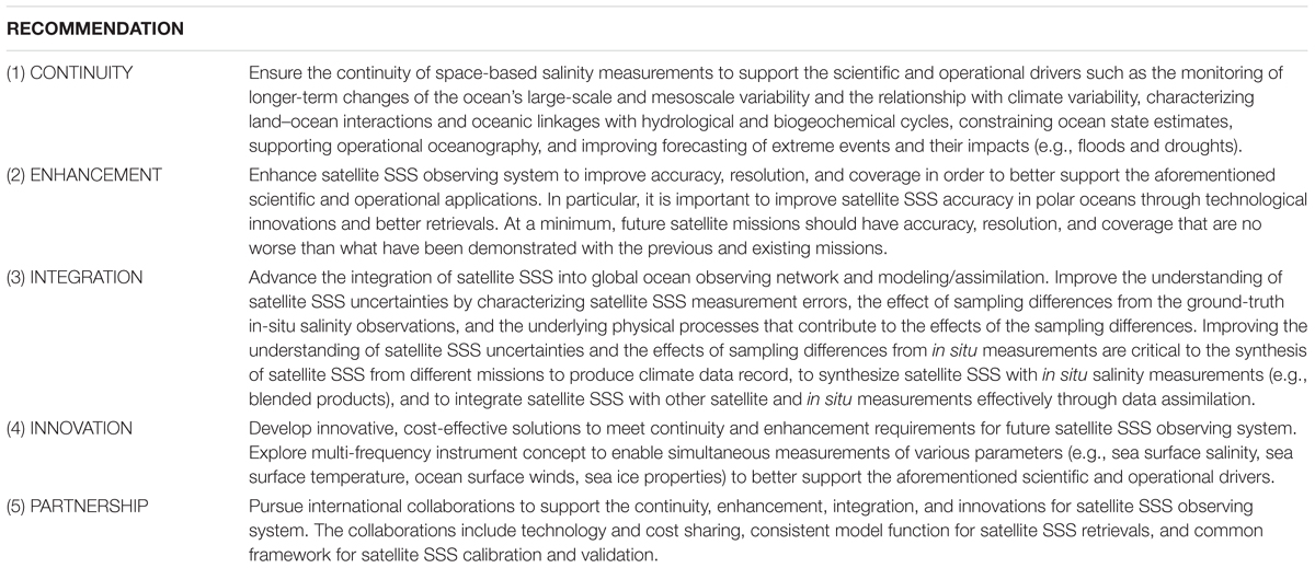
Table 1. Summary of recommendations for salinity remote sensing for next decade.

Author Contributions

NV and TL developed the conception of the review. All authors wrote the parts of various sections of the manuscript and contributed to the manuscript revision, read, and approved the submitted version.

Funding

Funding support by NASA Physical Oceanography Program is acknowledged.

Conflict of Interest Statement

The authors declare that the research was conducted in the absence of any commercial or financial relationships that could be construed as a potential conflict of interest.

The reviewer SG declared a past co-authorship with one of the authors NR, to the handling Editor.

Footnotes

1. ^Practical Salinity Scale 1978 (PSS-78) are used, following UNESCO guidelines “The Practical Salinity Scale 1978 and the International Equation of State of Seawater 1980.” Although salinities measured using PSS-78 do not have units, the suffix “pss” is sometimes used in the text and figures to distinguish the values of salinity, rates, and variance.
2. ^Other names have been also adopted in the community, with interchangeable use of “sampling” and “representation” errors; the latter is being more common in the modeling community. Observational errors have a variety of names, with most common being “measurement error,” “instrument noise,” “sensor noise,” and “data accuracy.”

References

Adam, O., Schneider, T., and Brient, F. (2018). Regional and seasonal variations of the double-ITCZ bias in CMIP5 models. Clim. Dyn. 51, 101–117. doi: 10.1007/s00382-017-3909-3901

CrossRef Full Text | Google Scholar

Akhil, V. P., Lengaigne, M., Vialard, J., Durand, F., Keerthi, M. G., Chaitanya, A. V. S., et al. (2016). A modeling study of processes controlling the Bay of Bengal sea surface salinity interannual variability. J. Geophys. Res. Oceans 121, 8471–8495. doi: 10.1002/2016JC011662

CrossRef Full Text | Google Scholar

Alory, G., Maes, C., Delcroix, T., Reul, N., and Illig, S. (2012). Seasonal dynamics of sea surface salinity off Panama: the far Eastern Pacific fresh pool. J. Geophys. Res. 117:C04028. doi: 10.1029/2011JC007802

CrossRef Full Text | Google Scholar

Bai, Y., Pan, D., Cai, W. J., He, X., Wang, D., Tao, B., et al. (2013). Remote sensing of salinity from satellite-derived CDOM in the Changjiang River dominated East China Sea. J. Geophys. Res. Oceans 118, 227–243.

Google Scholar

Bakker, D. C. E., Pfeil, B., Landa, C. S., and Metzl, N. (2016). A multi-decade record of high-quality fCO2 data in version 3 of the Surface Ocean CO2 Atlas (SOCAT). Earth Syst. Sci. Data 8, 383–413. doi: 10.5194/essd-8-383-2016

CrossRef Full Text | Google Scholar

Balaguru, K., Chang, P., Saravanan, R., Leung, L. R., Xu, Z., Li, M., et al. (2012). Ocean barrier layers’ effect on tropical cyclone intensification. PNAS 109, 14343–14347. doi: 10.1073/pnas.1201364109

PubMed Abstract | CrossRef Full Text | Google Scholar

Balaguru, K., Foltz, G. R., Leung, L. R., D’Asaro, E., Emanuel, K. A., Liu, H., et al. (2015). Dynamic potential intensity: an improved representation of the ocean’s impact on tropical cyclones. Geophys. Res. Lett 42, 6739–6746. doi: 10.1002/2015GL064822

CrossRef Full Text | Google Scholar

Balaguru, K., Foltz, G. R., Leung, L. R., and Emanuel, K. A. (2016). Global warming-induced upper-ocean freshening and the intensification of super typhoons. Nat. Commun. 7:13670. doi: 10.1038/ncomms13670

PubMed Abstract | CrossRef Full Text | Google Scholar

Banks, C. J., Srokosz, M. A., Cipollini, P., Snaith, H. M., Blundell, J. R., Gommenginger, C. P., et al. (2016). Reduced ascending/descending pass bias in SMOS salinity data demonstrated by observing westward-propagating features in the South Indian Ocean. Remote Sensing Environ. 180, 154–163. doi: 10.1016/j.rse.2016.02.035

CrossRef Full Text | Google Scholar

Belward, A., Bourassa, M. A., Dowell, M., and Briggs, S. (2016). The Global Observing System for climate: Implementation needs GCOS-200, https://unfccc.int/files/science/workstreams/systematic_observation/application/pdf/gcos_ip_10oct2016.pdf (accessed October 10, 2016).

Bingham, F. M., Busecke, J., Gordon, A. L., Giulivi, C. F., and Li, Z. (2014). The North Atlantic subtropical surface salinity maximum as observed by Aquarius. J. Geophys. Res. Oceans 119, 7741–7755. doi: 10.1002/2014JC009825

CrossRef Full Text | Google Scholar

Boukabara, S., Garrett, K., and Kumar, V. K. (2016). Potential Gaps in the satellite observing system coverage: assessment of impact on NOAA’s numerical weather prediction overall skills. Mon. Wea. Rev. 144, 2547–2563. doi: 10.1175/MWR-D-16-0013.1

CrossRef Full Text | Google Scholar

Boutin, J., Chao, Y., Asher, W. E., Delcroix, T., Drucker, R., Drushka, K., et al. (2016). Satellite and in situ salinity: understanding near-surface stratification and sub-footprint variability. Bull. Amer. Meteor. Soc 97, 1391–1407. doi: 10.1175/BAMS-D-15-00032.1

CrossRef Full Text | Google Scholar

Boutin, J., Vergely, J. L., Marchand, S., D’Amico, F., Hasson, A., Kolodziejczyk, N., et al. (2018). New SMOS Sea Surface Salinity with reduced systematic errors and improved variability. Remote Sens. Environ. 214, 115–134. doi: 10.1016/j.rse.2018.05.022

CrossRef Full Text | Google Scholar

Boyer, T. P., Levitus, S., Antonov, J. I., Locarnini, R. A., and Garcia, H. E. (2005). Linear trends in salinity for the World Ocean, 1955–1998. Geophys. Res. Lett. 32, L01604. doi: 10.1029/2004GL021791

CrossRef Full Text | Google Scholar

Brown, C. W., Boutin, J., and Merlivat, L. (2015). New insights of pCO2 variability in the tropical eastern Pacific Ocean using SMOS SSS. Biogeosciences 12, 7315–7329. doi: 10.5194/bg-12-7315-2015

CrossRef Full Text | Google Scholar

Brubaker, K. L., Entekhabi, D., and Eagleson, P. S. (1993). Estimation of continental precipitation recycling. J. Climate 6, 1077–1089.

Google Scholar

Busecke, J., Abernathey, R., and Gordon, A. (2017). Lateral eddy mixing in the subtropical salinity maxima of the global ocean. J. Phys. Oceanogr. 47, 737–754. doi: 10.1175/JPO-D-16-0215.1

CrossRef Full Text | Google Scholar

Canadell, J. G., Le Quéré, C., Raupach, M. R., Field, C. B., Buitenhuis, E. T., Ciais, P., et al. (2007). Contributions to accelerating atmospheric CO2 growth from economic activity, carbon intensity, and efficiency of natural sinks. PNAS 104, 18866–18870.

PubMed Abstract | Google Scholar

Carton, J. A., Chepurin, G. A., Chen, L., and Grodsky, S. A. (2018). Improved Global Net Surface Heat Flux. J. Geophys. Res. Oceans 123, 3144–3163. doi: 10.1002/2017JC013137

CrossRef Full Text | Google Scholar

Chakraborty, A., Kumar, R., Basu, S., and Sharma, R. (2015). Improving ocean state by assimilating SARAL/AltiKa derived sea level and other satellite-derived data in MITGCM. Mar. Geod. 38, 328–338. doi: 10.1080/01490419.2014.1002142

CrossRef Full Text | Google Scholar

Chan, S. C., and Misra, V. (2010). A diagnosis of the 1979-2005 extreme rainfall events in the Southeast US with isentropic moisture tracing. Mon. Wea. Rev. 138, 1172–1185.

Google Scholar

Chelton, D. B., deSzoeke, R. A. M., Schlax, G., El Naggar, K., and Siwertz, N. (1998). geographical variability of the first baroclinic rossby radius of deformation. J. Phys. Oceanogr. 28, 433–460.

Google Scholar

Chelton, D. B., Wentz, F. J., Gentemann, C. L., de Szoeke, R. A., and Schlax, M. G. (2000). Satellite microwave SST observations of trans equatorial tropical instability waves. Geophys. Res. Lett. 27, 1239–1242. doi: 10.1029/1999GL011047

CrossRef Full Text | Google Scholar

Cione, J. J., and Uhlhorn, E. W. (2003). Sea surface temperature variability in hurricanes: implications with respect to intensity change. Mon. Wea. Rev. 131, 1783-1796.

Google Scholar

Cook, B. I., Seager, R., and Miller, R. L. (2011). On the causes and dynamics of the early twentieth-century North American pluvial. J. Climate 24, 5043–5060.

Google Scholar

Cravatte, S., Delcroix, T., and Zhang, D. (2009). Observed freshening and warming of the western Pacific Warm Pool. Clim. Dyn. 33, 565. doi: 10.1007/s00382-009-0526-527

CrossRef Full Text | Google Scholar

Curry, R., Dickson, R., and Yashayaev, I. (2003). A change in the freshwater balance of the Atlantic Ocean over the past four decades. Nature 426, 826–829.

PubMed Abstract | Google Scholar

Da-Allada, C. Y., Jouanno, J., Gaillard, F., Kolodziejczyk, N., Maes, C., Reul, N. N., et al. (2017). Importance of the Equatorial Undercurrent on the sea surface salinity in the eastern equatorial Atlantic in boreal spring. J. Geophys. Res. Oceans 122, 521–538. doi: 10.1002/2016JC012342

CrossRef Full Text | Google Scholar

Delcroix, T. (1998). Observed surface oceanic and atmospheric variability in the tropical Pacific at seasonal and ENSO timescales: a tentative overview. J. Geophys. Res. 103, 18611–18633. doi: 10.1029/98JC00814

CrossRef Full Text | Google Scholar

Delcroix, T., Cravatte, S., and McPhaden, M. J. (2007). Decadal variations and trends in tropical Pacific sea surface salinity since 1970. J. Geophys. Res. 112:C03012. doi: 10.1029/2006JC003801

CrossRef Full Text | Google Scholar

Delcroix, T. M., McPhaden, J., Dessier, A., and Gouriou, Y. (2005). Time and space scales for sea surface salinity in the tropical oceans. Deep-Sea Res. 52, 787–813.

Google Scholar

Dirmeyer, P. A., Schlosser, C. A., and Brubaker, K. L. (2009). Precipitation, recycling, and land memory: an integrated analysis. J. Hydrometeor. 10, 278–288.

Google Scholar

Drucker, R., and Riser, S. C. (2014). Validation of Aquarius sea surface salinity with Argo: analysis of error due to depth of measurement and vertical salinity stratification. J. Geophys. Res. Oceans 119, 4626–4637.

Google Scholar

Drushka, K., Asher, W. E., Ward, B. B., and Walesby, K. (2016). Understanding the formation and evolution of rain-formed fresh lenses at the ocean surface. J. Geophys. Res. Oceans 121, 2673–2689. doi: 10.1002/2015JC011527

CrossRef Full Text | Google Scholar

Du, Y., and Zhang, Y. (2015). Satellite and argo observed surface salinity variations in the tropical indian ocean and their association with the Indian Ocean dipole mode. J. Climate 28, 695–713. doi: 10.1175/JCLI-D-14-00435.1

CrossRef Full Text | Google Scholar

Durack, P., Wijffels, S. E., and Boyer, T. P. (2013). “International Geophysics” in Long-term Salinity Changes and Implications for the Global Water Cycle, eds G., Siedler, S. M., Griffies, J., Gould, J. A., Church (Cambridge: Academic Press).

Durack, P. J. (2015). Ocean salinity and the global water cycle. Oceanography 28, 20–31. doi: 10.5670/oceanog.2015.03

Durack, P. J., Lee, T., Vinogradova, N. T., and Stammer, D. (2016). Keeping the lights on for global ocean salinity observation. Nat. Clim. Change 6, 228–231. doi: 10.1038/nclimate2946

CrossRef Full Text | Google Scholar

Durack, P. J., and Wijffels, S. E. (2010). Fifty-year trends in global ocean salinities and their relationship to broad-scale warming. J. Climate 23, 4342–4436.

Google Scholar

Durack, P. J., Wijffels, S. E., and Matear, R. J. (2012). Ocean Salinities Reveal Strong Global Water Cycle Intensification During 1950 to 2000. Science 336, 455–458. doi: 10.1126/science.1212222

PubMed Abstract | CrossRef Full Text | Google Scholar

Durand, F., Alory, G., Dussin, R., and Reul, N. (2013). SMOS reveals the signature of Indian Ocean Dipole events. Ocean Dynamics 63, 1203–1212. doi: 10.1007/s10236-013-0660-y

CrossRef Full Text | Google Scholar

Entekhabi, D., Njoku, E. G., O’Neill, P. E., Kellogg, K. H., Crow, W. T., Edelstein, W. N., et al. (2010). The soil moisture active passive (SMAP) mission. Proc. IEEE 98, 704–716.

Google Scholar

Entekhabi, D., Yueh, S., O’Neill, P. E., Kellogg, K. H., Allen, A., Bindlish, R., et al. (2014). SMAP handbook soil moisture active passive: Mapping soil moisture and freeze/thaw from space, JPL CL14-2285. Pasadena, CA: Jet Propulsion Laboratory.

Google Scholar

Ffield, A. (2007). Amazon and Orinoco river plumes and NBC rings: bystanders or participants in hurricane events? J. Climate 20, 316–333. doi: 10.1175/JCLI3985.1

CrossRef Full Text | Google Scholar

Fine, R. A., Willey, D. A., and Millero, F. J. (2017). Global variability and changes in ocean total alkalinity from Aquarius satellite data. Geophys. Res. Lett. 44, 261–267. doi: 10.1002/2016GL071712

CrossRef Full Text | Google Scholar

Foltz, G. R., and McPhaden, M. J. (2008). Seasonal mixed layer salinity balance of the tropical north Atlantic Ocean. J. Geophys. Res. 113:C02013. doi: 10.1029/2007JC004178

CrossRef Full Text | Google Scholar

Font, J., Camps, A., Borges, A., Martín-Neira, M., Boutin, J., Reul, N., et al. (2010). SMOS: the challenging sea surface salinity measurement from space. Proc. IEEE 98, 649–665.

Google Scholar

Fournier, S., Chapron, B., Salisbury, J., Vandemark, D., and Reul, N. (2015). Comparison of spaceborne measurements of Sea Surface Salinity and colored detrital matter in the Amazon plume. J. Geophys. Res. Oceans 3177–3192. doi: 10.1002/2014JC010109

CrossRef Full Text | Google Scholar

Fournier, S., Reager, J. T., Lee, T., Vazquez-Cuervo, J., David, C. H., and Gierach, M. M. (2016). SMAP observes flooding from land to sea: the Texas event of 2015. Geophys. Res. Lett. 43, 10338–10346. doi: 10.1002/2016GL070821

CrossRef Full Text | Google Scholar

Fournier, S., Reul, N., Charpon, B., and Tenerelli, J. (2011). Spatio-temporal coherence between spaceborne measurements of salinity and light absorption in the amazon plume region. in Proceedings of the ESA-SOLAS, Earth Observation for Ocean Atmosphere Interaction Science. Frascati: ESA Special Publication.

Fournier, S., Vandemark, D., Gaultier, L., Lee, T., Jonsson, B., and Gierach, M. M. (2017a). Interannual variation in offshore advection of Amazon-Orinoco plume waters: observations, forcing mechanisms, and impacts. J. Geophys. Res. Oceans 113. 122, 8966–8982. doi: 10.1002/2017JC013103

CrossRef Full Text | Google Scholar

Fournier, S., Vialard, J., Lengaigne, M., Lee, T., and Gierach, M. M. (2017b). Modulation of the Ganges-Brahmaputra river plume by the Indian Ocean Dipole and eddies inferred from satellite observations. J. Geophys. Res. Oceans 122, 9591–9604. doi: 10.1002/2017JC013333

CrossRef Full Text | Google Scholar

Friedman, A. R., Reverdin, G., Khodri, M., and Gastineau, G. (2017). A new record of Atlantic sea surface salinity from 1896 to 2013 reveals the signatures of climate variability and long-term trends. Geophys. Res. Lett. 44, 1866–1876. doi: 10.1002/2017GL072582

CrossRef Full Text | Google Scholar

Fukumori, I., Heimbach, P., Ponte, R. M., and Wunsch, C. (2018). A dynamically consistent, multi-variable ocean climatology. Bull. Amer. Meteor. Soc. 99, 2107–2128. doi: 10.1175/BAMS-D-17-0213.1

CrossRef Full Text | Google Scholar

Gierach, M. M., Vazquez Cuervo, J., Lee, T., and Tsontos, V. M. (2013). Aquarius and SMOS detect effects of an extreme Mississippi River flooding event in the Gulf of Mexico. Geophys. Res. Lett. 40, 5188–5193. doi: 10.1002/grl.50995

CrossRef Full Text | Google Scholar

Gimeno, L., Drumond, A., Nieto, R., Trigo, R. M., and Stohl, A. (2010). On the origin of continental precipitation. Geophys. Res. Lett. 37, L13804.

Google Scholar

Gimeno, L., Nieto, R., Drumond, A., Castillo, R., and Trigo, R. (2013). Influence of the intensification of the major oceanic moisture sources on continental precipitation. Geophys. Res. Lett. 40, 1–8.

Google Scholar

Gimeno, L., Stohl, A., Trigo, R. M., Dominguez, F., Yoshimura, K., Yu, L., et al. (2012). Oceanic and terrestrial sources of continental precipitation. Rev. Geophys. 50:RG4003.

Google Scholar

Glantz, M. H. (2001). Currents of Change: El Nino and La Nina Impacts on Climate and Society. Cambridge: Cambridge University Press.

Google Scholar

Gordon, A., and Giulivi, C. (2014). Ocean eddy freshwater flux convergence into the North Atlantic subtropics. J. Geophys. Res. Oceans 119, 3327–3335. doi: 10.1002/2013JC009596

CrossRef Full Text | Google Scholar

Gordon, A. L. (2016). The marine hydrological cycle: the ocean’s floods and droughts. Geophys. Res. Lett 43, 7649–7652. doi: 10.1002/2016GL070279

CrossRef Full Text | Google Scholar

Gordon, A. L., Giulivi, C. F., Busecke, J., and Bingham, F. M. (2015). Differences among subtropical surface salinity patterns. Oceanography 28, 32–39.

Google Scholar

Grodsky, S. A., and Carton, J. A. (2018). Delayed and quasi-synchronous response of tropical Atlantic surface salinity to rainfall. J. Geophys. Res. Oceans 123, 5971–5985. doi: 10.1029/2018JC013915

CrossRef Full Text | Google Scholar

Grodsky, S. A., Reul, N., Chapron, B., Carton, J. A., and Bryan, F. O. (2017). Interannual surface salinity in Northwest Atlantic shelf. J. Geophys. Res. Oceans 122, 3638–3659. doi: 10.1002/2016JC012580

PubMed Abstract | CrossRef Full Text | Google Scholar

Grodsky, S. A., Reul, N., Lagerloef, G., Reverdin, G., Carton, B., Chapron, J. A., et al. (2012). Haline hurricane wake in the Amazon/Orinoco plume: AQUARIUS/SACD and SMOS observations. Geophys. Res. Lett. 39:L20603.

Google Scholar

Grodsky, S. A., Reverdin, G., Carton, J. A., and Coles, V. J. (2014). Year-to-year salinity changes in the amazon plume: contrasting 2011 and 2012 aquarius/SACD and SMOS satellite data. Remote Sens. Environ. 140, 14–22. doi: 10.1016/j.rse.2013.08.033

CrossRef Full Text | Google Scholar

Grunseich, G., Subrahmanyam, B., and Wang, B. (2013). The Madden-Julian oscillation detected in Aquarius salinity observations. Geophys. Res. Lett. 40, 5461–5466. doi: 10.1002/2013GL058173

CrossRef Full Text | Google Scholar

Guan, B., Lee, T., Halkides, D. J., and Waliser, D. E. (2014). Aquarius surface salinity and the Madden-Julian oscillation: the role of salinity in surface layer density and potential energy. Geophys. Res. Lett. 41, 2858–2869. doi: 10.1002/2014GL059704

CrossRef Full Text | Google Scholar

Guerrero, R. A., Piola, A. R., Fenco, H., Matano, R. P., Combes, V., Chao, Y., et al. (2014). The salinity signature of the cross-shelf exchanges in the Southwestern Atlantic Ocean: satellite observations. J. Geophys. Res. Oceans 119, 7794–7810. doi: 10.1002/2014JC010113

PubMed Abstract | CrossRef Full Text | Google Scholar

Guimbard, S., Reul, N., Chapron, B., Umbert, M., and Maes, C. (2017). Seasonal and interannual variability of the Eastern Tropical Pacific Fresh Pool. J. Geophys. Res. Oceans 122, 1749–1771. doi: 10.1002/2016JC012130

CrossRef Full Text | Google Scholar

Hackert, E., Ballabrera-Poy, J., Busalacchi, A., Zhang, R. H., and Murtugudde, R. (2011). Impact of sea surface salinity assimilation on coupled forecasts in the tropical Pacific. J. Geophys Res. Oceans 116:C05009. doi: 10.1029/2010JC006708

CrossRef Full Text | Google Scholar

Hackert, E., Busalacchi, A. J., and Ballabrera-Poy, J. (2014). Impact of Aquarius sea surface salinity observations on coupled forecasts for the tropical Indo-Pacific Ocean. J. Geophys. Res. Oceans 119, 4045–4067. doi: 10.1002/2013jc009697

CrossRef Full Text | Google Scholar

Hasson, A., Boutin, J., Puy, M., Guilyardi, E., and Morrow, R. (2018). Northward pathway across the tropical North Pacific Ocean revealed by surface salinity: how do El Niño Anomalies Reach Hawaii? J. Geophys. Res 123:4. doi: 10.1002/2017JC013423

CrossRef Full Text | Google Scholar

Hasson, A., Delcroix, T., Boutin, J., Dussin, R., and Ballabrera Poy, J. (2014). Analyzing the 2010–2011 La Niña signature in the tropical Pacific sea surface salinity using in situ data, SMOS observations, and a numerical simulation. J. Geophys. Res. Oceans 119, 3855–3867. doi: 10.1002/2013JC009388

CrossRef Full Text | Google Scholar

Hasson, A., Delcroix, T., and Dussin, R. (2013). An assessment of the mixed layer salinity budget in the tropical Pacific Ocean. Observations and modeling (1990-2009). Ocean Dyn. 63, 179–194. doi: 10.1007/s10236-013-0596-592

CrossRef Full Text | Google Scholar

Helm, K. P., Bindoff, N. L., and Church, J. A. (2010). Changes in the global hydrological-cycle inferred from ocean salinity. Geophys. Res. Lett. 37:L18701. doi: 10.1029/2010GL044222

CrossRef Full Text | Google Scholar

Hernandez, O., Boutin, J., Kolodziejczyk, N., Reverdin, G., Martin, N., Gaillard, F., et al. (2014). SMOS salinity in the subtropical North Atlantic salinity maximum: 1. Comparison with Aquarius and in situ salinity. J. Geophys. Res. Oceans 119, 8878–8896. doi: 10.1002/2013JC009610

CrossRef Full Text | Google Scholar

Hoareau, N., Portabella, M., Lin, W., Ballabrera-Poy, J., and Turiel, A. (2018). Error characterization of sea surface salinity products using triple collocation analysis. IEEE T. Geosci. Remote 99, 1–9. doi: 10.1109/TGRS.2018.2810442

CrossRef Full Text | Google Scholar

Horel, J. D., and Wallace, J. M. (1981). Planetary-scale atmospheric phenomena associated with the southern oscillation. Mon. Weather Rev. 109, 813–829. doi: 10.1175/1520-04931981109<0813:psapaw>2.0.co;2

CrossRef Full Text | Google Scholar

Hosoda, S., Suga, T., Shikama, N., and Mizuno, K. (2009). Global surface layer salinity change detected by Argo and its implication for hydrological cycle intensification. J. Oceanogr. 65, 579. doi: 10.1007/s10872-009-0049-41

CrossRef Full Text | Google Scholar

Ibánhez, J. S. P., Flores, M., and Lefèvre, N. (2017). Collapse of the tropical and subtropical North Atlantic CO2 sink in boreal spring of 2010. Sci. Rep. 7:41694. doi: 10.1038/srep41694

PubMed Abstract | CrossRef Full Text | Google Scholar

Isern-Fontanet, J., Olmedo, E., Turiel, A., Ballabrera-Poy, J., and García-Ladona, E. (2016). Retrieval of eddy dynamics from SMOS sea surface salinity measurements in the Algerian Basin (Mediterranean Sea). Geophys. Res. Lett. 43, 6427–6434. doi: 10.1002/2016GL069595

CrossRef Full Text | Google Scholar

Kao, H. Y., and Lagerloef, G. S. E. (2018). Salinity Fronts in the Tropical Pacific Ocean. J. Geophys. Res. Oceans 120, 1096–1106. doi: 10.1002/2014JC010114

PubMed Abstract | CrossRef Full Text | Google Scholar

Kendall, B. M., Blume, H. J. C., and Cross, A. E. (1985). Development of UHF radiometer. Technical Report NASA-TP-2504. Hampton, VA: NASA Langley Research Center.

Google Scholar

Kerr, Y. H., Waldteufel, P., Wigneron, J. P., Martinuzzi, J. A. M. J., Font, J., and Berger, M. (2001). Soil moisture retrieval from space: the Soil Moisture and Ocean Salinity (SMOS) mission. IEEE Trans. Geosci. Remote Sens. 39, 1729–1735. doi: 10.3390/s100100584

PubMed Abstract | CrossRef Full Text | Google Scholar

Khatiwala, S., Primeau, F., and Hall, T. (2009). Reconstruction of the history of anthropogenic CO2 concentrations in the ocean. Nature 462, 346–349. doi: 10.1038/nature08526

PubMed Abstract | CrossRef Full Text | Google Scholar

Klein, L. A., and Swift, C. T. (1977). An Improved Model for the Dielectric Constant of Sea Water at Microwave Frequencies. IEEE J. Ocean. Eng. 2, 104–111. doi: 10.1109/JOE.1977.1145319

CrossRef Full Text | Google Scholar

Köhl, A., Stammer, D., and Sena-Martins, M. (2014). ). Impact of assimilating surface salinity from SMOS on ocean circulation estimates. J. Geophy. Res. 119, 5449–5464. doi: 10.1002/2014JC010040

CrossRef Full Text | Google Scholar

Kolodziejczyk, N., Hernandez, O., Boutin, J., and Reverdin, G. (2015). SMOS salinity in the subtropical North Atlantic salinity maximum: 2. Two-dimensional horizontal thermohaline variability. J. Geophys. Res. Oceans 120, 972–987. doi: 10.1002/2014JC010103

CrossRef Full Text | Google Scholar

Korosov, A., Counillon, F., and Johannessen, J. A. (2015). Monitoring the spreading of the Amazon freshwater plume by MODIS, SMOS, Aquarius, and TOPAZ. J. Geophys. Res. Oceans 120, 268–283. doi: 10.1002/2014JC010155

CrossRef Full Text | Google Scholar

Koster, R. D., Dirmeyer, P. A., Guo, Z., Bonan, G., Chan, E., Cox, P., et al. (2004). Regions of strong coupling between soil moisture and precipitation. Science 305, 1138–1140.

Google Scholar

Kunkel, K. E., Easterling, D. R., Kristovich, D. A. R., Gleason, B., Stoecker, L., and Smith, R. (2012). Meteorological causes of the secular variations in observed extreme precipitation events for the conterminous United States. J. Hydrometeor. 13, 1131–1141.

Google Scholar

Lagerloef, G., DeCharon, A., and Lindstrom, E. (2013). Ocean salinity and the aquarius/SAC-D Mission: a new frontier in ocean remote sensing. J. Mar. Technol. Soc. 47, 26–30.

Google Scholar

Lagerloef, G., Schimitt, R., Schanze, J., and Kao, H. Y. (2010). The ocean and the global water cycle. Oceanography 23, 82–93.

Google Scholar

Lagerloef, G. H., Kao, Y., Meissner, T., and Vazquez, J. (2015). Aquarius salinity Validation Analysis; Data Version 4.0, Aquarius Tech. Rep. AQ-014-PS-0016, PO. DAAC, JPL, NASA. Available at http://podaac.jpl.nasa.gov/SeaSurfaceSalinity/Aquarius (accessed August 2, 2015).

Lagerloef, G. S. E., Colomb, F. R., Le Vine, D., Wentz, F., Yueh, S., Ruf, C., et al. (2008). The Aquarius/SAC-D mission: designed to meet the salinity remote- sensing challenge. Oceanography 21, 68–81.

Google Scholar

Land, P. E., Shutler, J. D., Findlay, H. S., Girard-Ardhuin, F., Sabia, R., Reul, N., et al. (2015). Salinity from Space Unlocks Satellite-Based Assessment of Ocean Acidification. Environ. Sci. Technol. 49, 1987–1994. doi: 10.1021/es504849s

PubMed Abstract | CrossRef Full Text | Google Scholar

Le Quere, C., Raupach, M. R., Canadell, J. G., and Marlandet, G. (2009). Trends in the sources and sinks of carbon dioxide. Nat. Geosci. 2, 831–836.

Google Scholar

Le Traon, P. Y., Antoine, D., Bentamy, A., Bonekamp, H., Breivik, L. A., Chapron, B., et al. (2015). Use of satellite observations for operational oceanography: recent achievements and future prospects. J. Operat. Oceanogr. 8, 12–27. doi: 10.1080/1755876X.2015.1022050

CrossRef Full Text | Google Scholar

Le Vine, D. M., Abraham, S., Wentz, F., and Lagerloef, G. S. E. (2005). Impact of the Sun on remote sensing of sea surface salinity from space. Proc. Internat. Geosci. & Remote Sens. Sympos, IGARSS05 1, 288–291. doi: 10.1109/IGARSS.2005.1526164

CrossRef Full Text | Google Scholar

Le Vine, D. M., Lagerloef, G. S. E., Colomb, F. R., Yueh, S. H., and Pellerano, F. A. (2007). Aquarius: an instrument to monitor sea surface salinity from Space. in Proceedings of the IEEE Transactions on Geoscience and Remote Sensing (Seoul: IEEE).

Google Scholar

Lee, K., Tong, L. T., Millero, F. J., Sabine, C. L., Dickson, A. G., Goyet, C., et al. (2006). Global relationships of total alkalinity with salinity and temperature in surface waters of the world’s ocean. Geophys. Res. Lett. 33:L19605. doi: 10.1029/2006GL027207

CrossRef Full Text | Google Scholar

Lee, T. (2016). Consistency of Aquarius sea surface salinity with Argo products on various spatial and temporal scales. Geophys. Res. Lett. 43, 3857–3864. doi: 10.1002/2016GL068822

CrossRef Full Text | Google Scholar

Lee, T., Lagerloef, G., Gierach, M. M., Kao, H.-Y., Yueh, S., and Dohan, K. (2012). Aquarius reveals salinity structure of tropical instability waves. Geophys. Res. Lett. 39:L12610. doi: 10.1029/2012GL052232

CrossRef Full Text | Google Scholar

Lee, T., Lagerloef, G. S. E., Kao, H.-Y., McPhaden, M. J., Willis, J., and Gierach, M. M. (2014). The influence of salinity on tropical Atlantic instability waves. J. Geophys. Res. 119, 8375–8394. doi: 10.1002/2014JC010100

CrossRef Full Text | Google Scholar

Lee, T., Yueh, S., Lagerloef, G., Steele, M., Thompson, A., Flexas, M., et al. (2016). Linkages of salinity with ocean circulation, water cycle, and climate variability. Community white paper in response to Request for Information #2 by the US National Research Council Decadal Survey for Earth Science and Applications from Space 2017-2027. http://surveygizmoresponseuploads.s3.amazonaws.com/fileuploads/15647/2604456/107-1abc9aa1a37ab7e77d91d86598954a50_LeeTong.pdf (accessed May 14, 2019).

Lefèvre, N., Urbano, D. F., Gallois, F., and Diverrès, D. (2014). Impact of physical processes on the seasonal distribution of the fugacity of CO2 in the western tropical Atlantic. J. Geophys. Res. Oceans 119, 646–663. doi: 10.1002/2013JC009248

CrossRef Full Text | Google Scholar

Legeckis, R. V. (1977). Long waves in the eastern equatorial ocean. Science 197, 1177–1181.

PubMed Abstract

Li, L., Li, W., and Barros, A. P. (2013). Atmospheric moisture budget and its regulation of the summer precipitation variability over the Southeastern United States. Clim. Dyn. 41, 613–631.

Google Scholar

Li, L., Schmitt, R. W., and Ummenhofer, C. C. (2018). The role of the subtropical North Atlantic water cycle in recent US extreme precipitation events. Clim. Dyn. 50, 1291–1305.

Google Scholar

Li, L., Schmitt, R. W., Ummenhofer, C. C., and Karnauskas, K. B. (2016a). Implications of North Atlantic sea surface salinity for summer precipitation over the US Midwest: mechanisms and predictive values. J. Clim. 29, 3143–3159.

Google Scholar

Li, L., Schmitt, R. W., Ummehofer, C. C., and Karnauskas, K. B. (2016b). North Atlantic salinity as a predictor of Sahel rainfall. Sci. Adv. 2:e1501588. doi: 10.1126/sciadv.1501588

PubMed Abstract | CrossRef Full Text | Google Scholar

Li, Y., Han, W., and Lee, T. (2015). Intraseasonal sea surface salinity variability in the equatorial Indo-Pacific Ocean induced by Madden-Julian Oscillations. J. Geophys. Res. Oceans 120, 2233–2258. doi: 10.1002/2014JC010647

CrossRef Full Text | Google Scholar

Lindstrom, E., Bryan, F., and Schmitt, R. (2015). SPURS: salinity processes in the upper-ocean regional study—The North Atlantic experiment. Oceanography 28, 14–19. doi: 10.5670/oceanog.2015.01

CrossRef Full Text | Google Scholar

Liu, C., and Zipser, E. (2014). Differences between the surface precipitation estimates from the TRMM precipitation radar and passive microwave radiometer version 7 products. J. Hydrometeor. 15, 2157–2175. doi: 10.1175/JHM-D-14-0051.1

CrossRef Full Text | Google Scholar

Liu, T., Schmitt, R. W., and Li, L. (2018). Global search for autumn-lead sea surface salinity predictors of winter precipitation in southwestern United States. Geophys. Res. Lett. 45, 8445–8454.

Google Scholar

Lu, Z., Cheng, L., Zhu, J., and Lin, R. (2016). The complementary role of SMOS sea surface salinity observations for estimating global ocean salinity state. J. Geophys. Res. Oceans 121, 3672–3691.

Google Scholar

Lukas, R., and Lindstrom, E. (1991). The mixed layer of the western equatorial Pacific Ocean. J. Geophys. Res. 96, 3343–3357.

Google Scholar

Maes, C., Picaut, J., and Belamari, S. (2005). Importance of the salinity barrier layer for the buildup of El Niño. J. Clim. 18, 104–118.

Google Scholar

Maes, C., Reul, N., Behringer, D., and O’Kane, T. (2014). The salinity signature of the equatorial Pacific cold tongue as revealed by the satellite SMOS mission. Geosci. Lett. 1:17.

Google Scholar

Mahadevan, A., Jaeger, G. S., Freilich, M., Omand, M. M., Shroyer, E. L., and Sengupta, D. (2016). Freshwater in the Bay of Bengal: Its fate and role in air-sea heat exchange. Oceanography 29, 72–81.

Google Scholar

Martin, M. J., King, R. R., While, J., and Aguiar, A. (2018). Assimilating satellite sea surface salinity data from SMOS, Aquarius and SMAP into a global ocean forecasting system. Q. J. R. Meteorol. Soc. 145, 705–726. doi: 10.1002/qj.3461

CrossRef Full Text | Google Scholar

McKee, B., Aller, R., Allison, M., Bianchi, T., and Kineke, G. (2004). Transport and transformation of dissolved and particulate materials on continental margins influenced by major rivers: benthic boundary layer and seabed processes. Cont. Shelf Res. 24, 899–926. doi: 10.1016/j.csr.2004.02.009

CrossRef Full Text | Google Scholar

McPhaden, M. J., Zebiak, S. E., and Glantz, M. H. (2006). ENSO as an integrating concept in earth science. Science 1740–1745.

PubMed Abstract | Google Scholar

Meissner, T., Wentz, F., and Ricciardulli, L. (2014). The emission and scattering of L-band microwave radiation from rough ocean surfaces and wind speed measurements from Aquarius. J. Geophys. Res. Oceans 119, 6499–6522. doi: 10.1002/2014JC009837

CrossRef Full Text | Google Scholar

Meissner, T., Wentz, F. J., and Le Vine, D. M. (2018). The Salinity Retrieval Algorithms for the NASA Aquarius Version 5 and SMAP Version 3 Releases. Remote Sens. 10, 1121.

Google Scholar

Melnichenko, O., Amores, A., Maximenko, N., Hacker, P., and Potemra, J. (2017). Signature of mesoscale eddies in satellite sea surface salinity data. J. Geophys. Res. Oceans 122, 1416–1424. doi: 10.1002/2016JC012420

PubMed Abstract | CrossRef Full Text | Google Scholar

Melnichenko, O., Hacker, P., Maximenko, N., Lagerloef, G., and Potemra, J. (2014). Spatial optimal interpolation of aquarius sea surface salinity: algorithms and implementation in the north atlantic. J. Atmos. Oceanic Technol 31, 1583–1600. doi: 10.1175/JTECH-D-13-00241.1

CrossRef Full Text | Google Scholar

Melnichenko, O., Hacker, P., Maximenko, N., Lagerloef, G., and Potemra, J. (2016). Optimum interpolation analysis of Aquarius sea surface salinity. J. Geophys. Res. Oceans 121, 602–616. doi: 10.1002/2015JC011343

CrossRef Full Text | Google Scholar

Menezes, V. V., Vianna, M. L., and Phillips, H. E. (2014). Aquarius sea surface salinity in the South Indian Ocean: revealing annual-period planetary waves. J. Geophys. Res. Oceans 119, 3883–3908. doi: 10.1002/2014JC009935

CrossRef Full Text | Google Scholar

Misra, S., Johnson, J., Aksoy, M., Peng, J., Bradley, D., O’Dwyer, I., et al. (2013). “SMAP RFI mitigation algorithm performance characterization using airborne high-rate direct-sampled SMAPVEX 2012 data,” in Geoscience and Remote Sensing Symposium (IGARSS), (Melbourne VIC: IEEE International), 41–44.

Google Scholar

Misra, S., Kocz, J., Jarnot, R., Brown, S., Bendig, R., Felton, C., et al. (2018). Development of an On-board Wide-band Processor for Radio Frequency Interference Detection and Filtering. IEEE Trans. Geosci. Rem. Sens 1–13. doi: 10.1109/TGRS.2018.2882306

CrossRef Full Text | Google Scholar

Muller-Karger, F. E., McClain, C. R., and Richardson, P. L. (1988). The dispersal of the Amazon’s water. Nature 333, 56–59. doi: 10.1038/333056a0

CrossRef Full Text | Google Scholar

National Academies of Sciences, Engineering, and Medicine. (2016). Next Generation Earth System Prediction: Strategies for Subseasonal to Seasonal Forecasts. Washington, DC: The National Academies Press.

Google Scholar

Neetu, S., Lengaigne, M., Vincent, E. M., Vialard, J., Madec, G., Samson, G., et al. (2012). Influence of oceanic stratification on tropical cyclones-induced surface cooling in the Bay of Bengal. J. Geophys. Res. Oceans 117, C12020. doi: 10.1029/2012JC008433

CrossRef Full Text | Google Scholar

Oliva, R., Daganzo, E., Richaume, P., and Kerr, Y. (2016). Status of Radio Frequency Interference (RFI) in the 1400–1427MHz passive band based on six years of SMOS mission. Rem. Sens. Env. 180, 64–75.

Google Scholar

Olmedo, E., Taupier-Letage, I., Turiel, A., and Alvera-Azcárate, A. (2018). Improving SMOS sea surface salinity in the western Mediterranean sea through multivariate and multifractal analysis. Remote Sens. 10, 485.

Google Scholar

Pailler, K., Bourles, B., and Gouriou, Y. (1999). The barrier layer in the western tropical Atlantic Ocean. Geophys. Res. Lett. 26, 2069–2072. doi: 10.1029/1999GL900492

CrossRef Full Text | Google Scholar

Pawlowicz, R., Feistel, R., McDougall, T. J., Ridout, P., Seitz, S., and Wolf, H. (2016). Metrological challenges for measurements of key climatological observables, Part 2: oceanic salinity. Metrologia 53, R12–R25. doi: 10.1088/0026-1394/53/1/R12

CrossRef Full Text | Google Scholar

Piepmeier, J. R., Johnson, J. T., Mohammed, P. N., Bradley, D., Ruf, C., Aksoy, M., et al. (2014). Radio-frequency interference mitigation for the soil moisture active passive microwave radiometer. IEEE Trans. Geosci. Remote Sens. 52, 761–775.

Google Scholar

Pollard, R. T., and Regier, L. A. (1992). Vorticity and vertical circulation at the ocean front. J. Phys. Oceanogr. 22, 609–625. doi: 10.1371/journal.pone.0129045

PubMed Abstract | CrossRef Full Text | Google Scholar

Ponte, R. M., and Vinogradova, N. T. (2016). An assessment of basic processes controlling mean surface salinity over the global ocean. Geophys. Res. Lett. 43, 7052–7058. doi: 10.1002/2016GL069857

CrossRef Full Text | Google Scholar

Rao, R. R., and Sivakumar, R. (2003). Seasonal variability of the salt budget of the mixed layer and near-surface layer salinity structure of the tropical Indian Ocean from a new global ocean salinity climatology. J. Geophys. Res. Oceans 108:3009.

Google Scholar

Reul, N., Chapron, B., Lee, T., Donlon, C., Boutin, J., and Alory, G. (2014a). Sea surface salinity structure of the meandering Gulf Stream revealed by SMOS sensor. Geophys. Res. Lett. 41, 3141–3148. doi: 10.1002/2014GL059215

CrossRef Full Text | Google Scholar

Reul, N., Quilfen, Y., Chapron, B., Fournier, S., Kudryavtsev, V., and Sabia, R. (2014b). Multisensor observations of the Amazon-Orinoco river plume interactions with hurricanes. J. Geophys. Res. Oceans 119, 8271–8295. doi: 10.1002/2014JC010107

CrossRef Full Text | Google Scholar

Reul, N., Fournier, S., Boutin, J., Hernandez, O., Maes, C., Chapron, B., et al. (2013). Sea surface salinity observations from space with the SMOS satellite: a new means to monitor the marine branch of the water cycle. Surv. Geophy. 35, 681–722. doi: 10.1007/s10712-013-9244-0

CrossRef Full Text | Google Scholar

Reul, N., Tenerelli, J., Chapron, B., Vandemark, D., Quilfen, Y., and Kerr, Y. (2012). SMOS satellite L-band radiometer: a new capability for ocean surface remote sensing in hurricanes. J. Geophys. Res. 117:C02006. doi: 10.1029/2011JC007474

CrossRef Full Text | Google Scholar

Reul, N., Tenerelli, J., Chapron, B., and Waldteufel, P. (2007). Modeling sun glitter at l-band for sea surface salinity remote sensing with SMOS. IEEE Trans. Geosci. Remote Sens. 45, 2073–2087.

Google Scholar

Reul, N., Tenerelli, J., Floury, N., and Chapron, B. (2008). Earth-viewing L-band radiometer sensing of sea surface scattered celestial sky radiation. part II: application to SMOS. IEEE Trans. Geosci. Remote Sens. 46, 675–688.

Google Scholar

Ruf, C. S., Gross, S. M., and Misra, S. (2006). RFI detection and mitigation for microwave radiometry with an agile digital detector. IEEE Trans. Geosci. Remote Sens. 44, 694–706.

Google Scholar

Sabia, R., Fernández-Prieto, D., Shutler, J., Donlon, C., Land, P., and Reul, N. (2015a). Remote sensing of surface ocean PH exploiting sea surface salinity satellite observations in Proceedings of the IEEE International Geoscience and Remote Sensing Symposium. Milan: IEEE.

Sabia, R., Klockmann, M., Fernández-Prieto, D., and Donlon, C. (2015b). Air-sea fluxes and satellite-based estimation of water masses formation. Geophy. Res. Abs. 17:EGU2015–EGU13074.

Google Scholar

Sabine, C. L., Feely, R. A., Gruber, N., Key, R. M., Bullister, J. L., Wanninkhof, R., et al. (2004). The oceanic sink for anthropogenic CO2. Science 305, 367–371.

Google Scholar

Saji, N. H., Goswami, B. N., Vinayachandran, P. N., and Yamagata, T. (1999). A dipole mode in the tropical Indian Ocean. Nature 401, 360–363.

Google Scholar

Salisbury, J., Vandemark, D., Jönsson, B., Balch, W., Chakraborty, S., Lohrenz, S., et al. (2015). How can present and future satellite missions support scientific studies that address ocean acidification? Oceanography 28, 108–121. doi: 10.5670/oceanog.2015.35

CrossRef Full Text | Google Scholar

Schanze, J. J., Schmitt, R. W., and Yu, L. L. (2010). The global oceanic freshwater cycle: a state-of-the-art quantification. J. Mar. Res. 68, 569–595.

Google Scholar

Schmitt, R. W. (1995). The ocean component of the global water cycle. Rev. Geophys. 33, 1395–1409.

Google Scholar

Schmitt, R. W. (2008). Salinity and the global water cycle. Oceanography 21, 12–19.

Google Scholar

Seager, R., and Vecchi, G. A. (2010). Greenhouse warming and the 21st century hydroclimate of southwestern North America. Proc. Natl. Acad. Sci. U.S.A. 107, 21277–21282. doi: 10.1073/pnas.0910856107

PubMed Abstract | CrossRef Full Text | Google Scholar

Sengupta, D., Goddalehundi, B. R., and Anitha, D. S. (2008). Cyclone-induced mixing does not cool SST in the post-monsoon North Bay of Bengal. Atm. Sci. Lett. 9, 1–6. doi: 10.1002/asl.162

CrossRef Full Text | Google Scholar

Shenoi, S. S. C., Shankar, D., and Shetye, S. R. (2002). Difference in heat budgets of the near-surface Arabian Sea and Bay of Bengal: implications for the summer monsoon. J. Geophys. Res. Oceans 107, 5–14. doi: 10.1029/2000JC000679

CrossRef Full Text | Google Scholar

Skliris, N., Marsh, R., Josey, S. A., Good, S. A., Liu, C., and Allan, R. P. (2014). Salinity changes in the World Ocean since 1950 in relation to changing surface freshwater fluxes. Clim. Dyn. 43, 709. doi: 10.1007/s00382-014-2131-2137

CrossRef Full Text | Google Scholar

Skliris, N., Zika, J. D., Nurser, G., Josey, S. A., and Marsh, R. (2016). Global water cycle amplifying at less than the Clausius-Clapeyron rate. Sci. Rep. 6, 752. doi: 10.1038/srep38752

PubMed Abstract | CrossRef Full Text | Google Scholar

Sommer, A., Reverdin, G., Kolodziejczyk, N., and Boutin, J. (2015). Sea surface salinity and temperature budgets in the North Atlantic subtropical gyre during SPURS experiment: August 2012-August 2013. Front. Mar. Sci. 2:107. doi: 10.3389/fmars.2015.00107

CrossRef Full Text | Google Scholar

SPURS-2 Planning Group. (2015). From salty to fresh—salinity processes in the upper-ocean regional study-2 (SPURS-2): diagnosing the physics of a rainfall-dominated salinity minimum. Oceanography 28, 150–159. doi: 10.5670/oceanog.2015.15

CrossRef Full Text | Google Scholar

Stammer, D. M., Balmaseda, P., Heimbach, A., Köhl, A., and Weaver, A. (2016). Ocean data assimilation in support of climate applications: status and perspectives. Ann. Rev. Mar. Sci. 8, 491–518. doi: 10.1146/annurev-marine-122414-034113

PubMed Abstract | CrossRef Full Text | Google Scholar

Stammer, D., Ueyoshi, K., Köhl, A., Large, W. G., Josey, S. A., and Wunsch, C. (2004). Estimating air-sea fluxes of heat, freshwater, and momentum through global ocean data assimilation. J. Geophys. Res. 109:C05023. doi: 10.1029/2003JC002082

CrossRef Full Text | Google Scholar

Stammer, D., Wunsch, C., Giering, R., Eckert, C., Heimbach, P., Marotzke, J., et al. (2002b). The global ocean circulation during 1992 –1997, estimated from ocean observations and a general circulation model. J. Geophys. Res. 107:3118. doi: 10.1029/2001JC000888

CrossRef Full Text | Google Scholar

Stammer, D., Wunsch, C., Fukumori, I., and Marshall, J. (2002a). State estimation improves prospects for ocean research. EOS AGU Trans. 83, 289–295.

Google Scholar

Stohl, A., and James, P. (2005). A Lagrangian analysis of the atmospheric branch of the global water cycle. Part II: Moisture transports between Earth’s ocean basins and river catchments. J. Hydrometeor. 6, 961–984.

Google Scholar

Stott, P. A., Sutton, R. T., and Smith, D. M. (2008). Detection and attribution of Atlantic salinity changes. Geophys. Res. Lett. 35:L21702. doi: 10.1029/2008GL035874

CrossRef Full Text | Google Scholar

Su, Z., Wang, J., Klein, P., Thompson, A. F., and Menemenlis, D. (2018). Ocean submesoscales as a key component of the global heat budget. Nat. Commun. 9, 775. doi: 10.1038/s41467-018-02983-w

PubMed Abstract | CrossRef Full Text | Google Scholar

Subrahmanyam, B., Trott, B. C., and Murty, V. S. N. (2018). Detection of intraseasonal oscillations in SMAP salinity in the Bay of Bengal. Geophys. Res. Lett. 45, 7057–7065. doi: 10.1029/2018GL078662

CrossRef Full Text | Google Scholar

Supply, A., Boutin, J., Vergely, J., Martin, N., Hasson, A., Reverdin, G., et al. (2017). Precipitation estimates from SMOS sea-surface salinity. Q. J. R. Meteorol. Soc 144, 103–119. doi: 10.1002/qj.3110

CrossRef Full Text | Google Scholar

Swift, C. T., and Mcintosh, R. E. (1983). Considerations for microwave remote sensing of ocean-surface salinity. IEEE Trans. Geosci. Remote Sens. 4, 480–491.

Google Scholar

Tang, W., Fore, A., Yueh, S., Lee, T., Hayashi, A., Sanchez-Franks, A., et al. (2017). Validating SMAP SSS with in-situ measurements. Rem. Sens. Environ. 200, 326–340. doi: 10.1016/j.rse.2017.08.021

CrossRef Full Text | Google Scholar

Tang, W., Yueh, S., Fore, A., Neumann, G., Hayashi, A., and Lagerloef, G. (2013). The rain effect on Aquarius’ L-band sea surface brightness temperature and radar backscatter. Remote Sens. Environ. 137, 147–157.

Google Scholar

Tang, W., Yueh, S. H., Fore, A. G., and Hayashi, A. A. (2014). Validation of Aquarius sea surface salinity with in situ measurements from Argo floats and moored buoys. J. Geophys. Res. Oceans 119, 6171–6189.

Google Scholar

Terray, L., Corre, L., Cravatte, S., Delcroix, T., Reverdin, G., and Ribes, A. (2012). Near-surface salinity as nature’s rain gauge to detect human influence on the tropical water cycle. J. Climate 25, 958–977. doi: 10.1175/JCLI-D-10-05025.1

CrossRef Full Text | Google Scholar

Thadathil, P., Suresh, I., Gautham, S., Prasanna Kumar, S., Lengaigne, M., Akshay, H., et al. (2016). Intraseasonal to interannual variability of surface layer temperature inversion in the Bay of Bengal: main characteristics and related mechanisms. J. Geophys. Res. 121, 5682–5696. doi: 10.1002/2016JC011674

CrossRef Full Text | Google Scholar

Toyoda, T., Fujii, Y., Kuragano, T., Matthews, J. P., Abe, H., Ebuchi, N., et al. (2015). Improvements to a global ocean data assimilation system through the incorporation of aquarius surface salinity data. Q. J. Roy. Meteor. Soc. 141, 2750–2759. doi: 10.1002/qj.2561

CrossRef Full Text | Google Scholar

Trenberth, K. E. (1998). Atmospheric moisture residence times and cycling: implications for rainfall rates and climate change. Clim. Change 39, 667–694.

Google Scholar

Trenberth, K. E. (1999). Atmospheric moisture recycling: role of advection and local evaporation. J. Climate 12, 1368–1381.

Google Scholar

Trenberth, K. E., and Guillemot, C. J. (1995). Evaluation of the global atmospheric moisture budget as seen from analyses. J. Climate 8, 2255–2272. doi: 10.1016/j.jes.2015.01.015

PubMed Abstract | CrossRef Full Text | Google Scholar

Trenberth, K. E., Smith, L., Qian, T., Dai, A., and Fasullo, J. (2007). Estimates of the global water budget and its annual cycle using observational and model data. J. Hydrometeor. 8, 758–769.

Google Scholar

van der Ent, R. J., Savenije, H. H. G., Schaefli, B., and Steele-Dunne, S. C. (2010). Origin and fate of atmospheric moisture over continents. Water Resour. Res. 46:W09525.

Google Scholar

Vialard, J., and Delecluse, P. (1998). An OGCM study for the TOGA decade. Part I: role of salinity in the physics of the western pacific fresh pool. J. Phys. Ocaenogr. 28, 1071–1088. doi: 10.1175/1520-04851998028<1071:AOSFTT>2.0.CO;2

CrossRef Full Text | Google Scholar

Vincent, E. M., Lengaigne, M., Madec, G., Vialard, J., Samson, G., Jourdain, N. C., et al. (2012). Processes setting the characteristics of sea surface cooling induced by tropical cyclones. J. Geophys. Res. 117:C02020. doi: 10.1029/2011JC007396

CrossRef Full Text | Google Scholar

Vinogradova, N. T. (2018). Synergistic use of satellite and in situ observations for production of multi-platform ocean state estimates for climate research. NASA Hyperwall Lecture Series. Available at: https://svs.gsfc.nasa.gov/hyperwall/index/download/events/2018-oceansciences/

Vinogradova, N. T., and Ponte, R. M. (2012). Assessing temporal aliasing in satellite-based salinity measurements. J. Atmos. Oceanic Tech. 29, 1391–1400.

Google Scholar

Vinogradova, N. T., and Ponte, R. M. (2013a). Clarifying the link between surface salinity and freshwater fluxes on monthly to interannual time scales. J. Gephys. Res. 118, 2190–3201. doi: 10.1002/jgrc.20200

CrossRef Full Text | Google Scholar

Vinogradova, N. T., and Ponte, R. M. (2013b). Small-scale variability in sea surface salinity and implications for satellite-derived measurements. J. Atmos. Oceanic Tech. 30, 2689–2694. doi: 10.1175/JTECH-D-13-00110.1

CrossRef Full Text | Google Scholar

Vinogradova, N. T., and Ponte, R. M. (2017). In search of fingerprints of the recent intensification of the ocean water cycle. J. Clim. 30, 5513–5528. doi: 10.1175/JCLI-D-16-0626.1

CrossRef Full Text | Google Scholar

Vinogradova, N. T., Ponte, R. M., Fukumori, I., and Wang, O. (2014). Estimating satellite salinity errors for assimilation of Aquarius and SMOS data into climate models. J. Geophys. Res. Oceans 119, 4732–4744. doi: 10.1002/2014JC009906

CrossRef Full Text | Google Scholar

Vizy, E. K., and Cook, K. H. (2010). Influence of the Amazon/Orinoco Plume on the summertime Atlantic climate. J. Geophys Res. Oceans 115, doi: 10.1029/2010JD014049

CrossRef Full Text | Google Scholar

Wang, W., Chen, M., and Kumar, A. (2010). An assessment of the CFS real-time seasonal forecasts. Weather Forecast. 25, 950–969. doi: 10.1175/2010waf2222345.1

CrossRef Full Text | Google Scholar

Weaver, S. J., and Nigam, S. (2008). Variability of the great plains low-level jet: large-scale circulation context and hydroclimate impacts. J. Climate 21, 1532–1551.

Google Scholar

Weaver, S. J., Ruiz-Barradas, A., and Nigam, S. (2009a). Pentad evolution of the 1988 drought and 1993 flood over the great plains: an NARR perspective on the atmospheric and terrestrial water balance. J. Climate 22, 5366–5384.

Google Scholar

Weaver, S. J., Schubert, S., and Wang, H. (2009b). Warm season variations in the low-level circulation and precipitation over the central United States in observations. AMIP simulations, and idealized SST experiment. J. Clim. 22, 5401–5420.

Google Scholar

Wood, H. C., Robar, J. D., Kavadas, A., and Vandall, P. E. Jr. (1975). The Remote Measurement of Water Salinity Using RF Radiometer Techniques. Can. J. Remote Sens. 1, 67–69.

Google Scholar

Woodson, C. B., and Litvin, S. Y. (2015). Ocean fronts drive marine fishery production and biogeochemical cycling. Proc. Natl. Acad. Sci. U.S.A. 112, 1710–1715. doi: 10.1073/pnas.1417143112

PubMed Abstract | CrossRef Full Text | Google Scholar

Wunsch, C. (2015). Modern Observational Physical Oceanography. New Jersey, NJ: Princeton University Press.

Google Scholar

Wunsch, C., Heimbach, P., and J. (2013). “Dynamically and kinematically consistent global ocean circulation and ice state estimates,” in Ocean Circulation and Climate: A 21 Century Perspective, eds G., Siedler, S., M. Griffies, and J. A., Church (Oxford, UK: Academic Press).

Google Scholar

Xie, P., Boyer, T., Bayler, E., Xue, Y., Byrne, D., Reagan, J., et al. (2014). An in situ-satellite blended analysis of global sea surface salinity. J. Geophys. Res. Oceans 119, 6140–6160. doi: 10.1002/2014JC010046

CrossRef Full Text | Google Scholar

Yin, X., Boutin, J., Reverdin, G., Lee, T., Arnault, S., and Martin, N. (2014). SMOS sea surface salinity signals of tropical instability waves. J. Geophys. Res. Oceans 119, 7811–7826. doi: 10.1002/2014JC009960

CrossRef Full Text | Google Scholar

Yu, L. (2011). A global relationship between the ocean water cycle and near-surface salinity. J. Geophys. Res. 116:C10025. doi: 10.1029/2010JC006937

CrossRef Full Text | Google Scholar

Yu, L. (2014). Coherent evidence from Aquarius and Argo for the existence of a shallow low-salinity convergence zone beneath the Pacific ITCZ. J. Geophys. Res. Oceans 119, 7625–7644. doi: 10.1002/2014JC010030

CrossRef Full Text | Google Scholar

Yu, L. (2015). Sea-surface salinity fronts and associated salinity minimum zones in the tropical ocean. J. Geophys. Res. Oceans 120, 4205–4225. doi: 10.1002/2015JC010790

CrossRef Full Text | Google Scholar

Yueh, S., Tang, W., Fore, A., Hayashi, A., Song, Y. T., and Lagerloef, G. (2014). Aquarius geophysical model function and combined active passive algorithm for ocean surface salinity and wind retrieval. J. Geophys. Res. Oceans 119, 5360–5379.

Google Scholar

Yueh, S., Tang, W., Fore, A., Neumann, G., Hayashi, A., Freedman, A., et al. (2013). L-band passive and active microwave geophysical model functions of ocean surface winds and applications to Aquarius retrieval. IEEE Trans. Geosci. Remote Sens. 51, 4619–4632.

Google Scholar

Yueh, S. H., Dinardo, S., Fore, A., and Li, F. (2010). Passive and Active L-Band Microwave Observations and Modeling of Ocean Surface Winds. IEEE Trans. Geosci. Remote Sens. 48, 3087–3100.

Google Scholar

Zeng, L., Liu, T., Xue, H., Xiu, P., and Wang, D. (2014). Freshening in the South China Sea during 2012 revealed by Aquarius and in situ data. J. Geophys. Res. Ocens 119, 8296–8314. doi: 10.1002/2014JC010108

CrossRef Full Text | Google Scholar

Zhang, C. (2005). Madden-Julian Oscillation. Rec. Geophys. 43:RG2003. doi: 10.1029/2004RG000158

CrossRef Full Text | Google Scholar

Zhou, T., and Yu, R. (2005). Atmospheric water vapor transport associated with typical anomalous summer rainfall patterns in China. J. Geophys. Res. Atmos. 110:D08104.

Google Scholar

Zhu, J., Huang, B., Rong-Hua, Z., Zeng-Zhen, H., Kumar, A., Balmaseda, M. A., et al. (2014). Salinity anomaly as a trigger for ENSO events. Sci. Rep. 4:6821. doi: 10.1038/srep06821

PubMed Abstract | CrossRef Full Text | Google Scholar

Zika, J. D., Skliris, N., Blaker, A. T., Marsh, R., Nurser, A. G., and Josey, S. A. (2018). Improved estimates of water cycle change from ocean salinity: the key role of ocean warming. Environ. Res. Lett. 13, 1–10. doi: 10.1088/1748-9326/aace42

CrossRef Full Text | Google Scholar