Trophic Interactions, Management Trade-Offs and Climate Change: The Need for Adaptive Thresholds to Operationalize Ecosystem Indicators

Introduction

Reduced impacts of human activities and sustainable use of marine natural resources is an urgent calling when other severe pressures on coastal and ocean systems, such as climate change, can only be curbed on long time-scales (Dayton et al., 1995; Worm et al., 2006; Field et al., 2014; Cloern et al., 2016). Ecosystem-based management (EBM) makes sustainable use achievable by taking an integrated perspective on multiple uses and different components of ecosystems (Rosenberg and McLeod, 2005; Leslie and McLeod, 2007). To ensure success, EBM needs to include initial and regular update assessments of the status of the ecosystem as well as evaluate the response to management measures and their efficiencies. Integrated ecosystem assessments (IEAs) provide a scientific basis for decision-making within EBM (Levin et al., 2009) where carefully selected indicators constitute the basis for status assessments and management strategy evaluations.

Typically, IEAs make use of several indicators to assess the state of the ecosystem, each representing some component or aspect of the ecosystem (e.g., Ottersen et al., 2011). The strong ecological linkages present in many ecosystems will often make indicators interlinked, e.g., in a food web due to species interactions (Håkanson and Blenckner, 2008). Therefore, management measures or pressures do not only act on one monitored indicator directly, but also indirectly on others (Torres et al., 2017). Consequently, when developing indicators and IEA frameworks, it is rarely sufficient to understand relationships between single pressures and single indicators, but joint analyses of multiple indicators are needed. This is true particularly for food-web indicators that represent different trophic guilds, which may integrate direct as well as indirect effects of pressures propagating through the food web. Overfishing of predatory fish for example, often results in marked increases of pelagic forage fish and benthic macroinvertebrates, in turn reducing biomass of zooplankton and subsequently consumption of phytoplankton (Frank et al., 2005; Casini et al., 2008). Other trophic cascades induced by fisheries have led to loss of, e.g., kelp forests as well as sea grass meadows and make ecosystems sensitive to disturbance (Jackson et al., 2001). Such mechanisms may amplify or exaggerate effects of eutrophication, thereby interfering with efforts to reduce nutrient loads, as well as signals of their success, typically tracked by indicators. Conversely, bottom-up dynamics can result in positive impacts of eutrophication on species benefitting from higher ecosystem productivity (Laursen and Moller, 2014). Trophic interactions may thus create trade-offs between management objectives, constrain achievable target levels for indicators or affect evaluations of management strategies as well as of specific measures to move the ecosystem toward a healthy state (Shelton et al., 2014; Punt et al., 2016).

Climate conditions are key pressures acting on ecosystems, with potential to influence management pathways or the effort required to improve their status (Niiranen et al., 2013). Quantitative evaluations of the interplay between climate and management measures on indicators are yet sparse, despite international and national legislations requiring the implementation of EBM and the large number of frameworks to develop operational indicators. Projected climate change may further amplify or dampen effects, and is thus necessary to account for when assessing the benefits of management measures (Lynam and Mackinson, 2015). Existing studies of indicators that account for climate change typically focus on effects of single drivers (Gårdmark et al., 2013), but EBM strives to balance multiple objectives, and management measures motivated by different objectives will thus be implemented simultaneously rather than in isolation. How do indicators respond to management alternatives when measures affecting top-down and bottom-up processes are implemented simultaneously under a changing climate? Indirect effects mediated by food-web interactions may be particularly difficult to foresee and could have a substantial impact on the interpretation of indicators.

In this study, we examine how indicators track effects of management strategies targeting different pressures on marine food webs under climate change, accounting for the interactions among species that constitute them. Using food-web indicators proposed for the Baltic Sea under the European Marine Strategy Framework Directive (MSFD), we apply advanced statistical modeling tools to identify indicator networks (Llope et al., 2011; Blenckner et al., 2015; Lynam et al., 2017, Figure 1). The indicator networks allow us to evaluate links between indicators, suggesting potential for cascading effects of management measures, and if these links magnify or counterbalance indicator responses to (single and multiple) pressures. Our approach illustrates how effects of climate change may interfere with effects of potential measures as manifested in the indicators. Such interactions change the interpretation of indicator responses in relation to reference points. By including indicators representing different trophic guilds and simultaneously modeling management measures targeting different pressures, our indicator networks aid in identification and quantification of potential trade-offs in EBM. We discuss strategies in EBM to detect and handle conflicts between objectives that arise due to trophic interactions, as well as modulating effects of climate change. Adaptive targets and thresholds are proposed as one approach to these challenges.

FIGURE 1

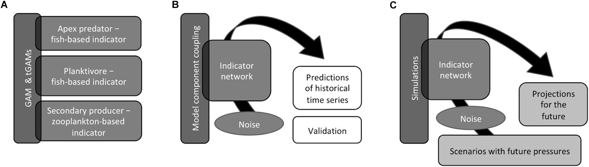
Figure 1. Representation of the three steps included in the modeling approach: (A) Model selection (Generalized Additive Models, GAMs, or their threshold-formulations, tGAMs) for each indicator. (B) Coupling of the selected models, where links between indicators were identified, into indicator networks to simulate past dynamics using residuals from individual models for uncertainty estimation. Predictions from networks were compared to observed values, from time-series used for fitting as well as a 3-year-validation period. (C) Indicator networks were used for simulations of future scenarios where we evaluated effects of manageable pressures and climate change on indicator responses and interpretation of indicators. See “Materials and Methods” and Supplementary Information: Appendix I for further details.

Materials and Methods

Study System and Selected Zooplankton and Fish Indicators

The study focused on food-web indicators of trophic functions in the pelagic food web of the Central Baltic Sea, a relatively simple brackish-water ecosystem, where recent impacts of fisheries and eutrophication in combination with climate factors have resulted in substantial ecological changes (Österblom et al., 2007). A regime shift occurred in the Central Baltic Sea in the early 1990s with effects cascading through the food web (Casini et al., 2008; Möllmann et al., 2009). Environmental gradients are prominent in the Baltic Sea and the recent changes have had, quantitatively and qualitatively, different impacts in the basins (Casini et al., 2011). We therefore used indicators of food-web status developed separately for the Bornholm and Gotland Basins (corresponding to ICES subdivisions 25 and 28, respectively, Supplementary Figure S1). At the trophic levels of zooplanktivorous and piscivorous fish, indicators of trophic functions correspond to single or only a few species in the species-poor system of the Baltic Sea (ICES, 2015c,d; Torres et al., 2017). The zooplankton community includes a substantially larger number of species and we derived indicators of the community representing aspects of quantity and quality of food for upper trophic levels. The indicators were considered for assessment under the ‘Baltic Sea Action Plan’ and descriptor 4 – food webs – of good environmental status in the MSFD and showed a good performance when studied individually (HELCOM, 2013a,b; Otto et al., 2018). Assessments under descriptor 4 are based on trophic guilds and our indicators covered three guilds: apex fish predators, planktivorous fish, and secondary producers; and three of four assessment criteria (EU Decision 2017/848; ICES, 2015b).

Historical Data and Indicator Time Series Construction

Data on piscivorous and planktivorous fish, representing the apex predator guild and the planktivore trophic guild, respectively, were obtained from the autumn Baltic International Acoustic Survey (BIAS, ICES, 2015a) and historical acoustic surveys by the Swedish University of Agricultural Sciences and the former Swedish Board of Fisheries. We calculated fish indicators based either on actual abundance (for sprat Sprattus sprattus and herring Clupea harengus) or modeled Catch Per Unit of Effort (CPUE) (for cod Gadus morhua; Casini et al., 2019) in the surveys (Cod, Sprat, Herring – collectively referred to as abundance-FI) and two indicators based on body size (Small Prey Fish, SPF, forage fish <10 cm; and Large Predatory Fish, LPF; piscivores > 38 cm – as size-based FI), according to the approach described in Torres et al. (2017). One initially considered indicator, CPUE of three-spined stickleback Gasterosteus aculeatus (Stickleback), was tested as a pressure variable, representing additional competition or predation depending on trophic level. Zooplankton-based indicators, corresponding to the secondary producer trophic guild, are collectively referred to as ZPI. This set of ZPI included total zooplankton abundance (TZA), zooplankton mean size (MS), and abundance ratio of cladocerans to copepods (excluding nauplii, RCC). Bornholm Basin ZPI were based on summer samples (average of July–August) taken at the BY5 station (55.25°N, 15.98°E) collected by the Leibniz Institute for Baltic Sea Research Warnemünde, Germany. Gotland Basin ZPI were calculated from summer samples (average of July–August) taken at multiple stations in seven ICES rectangles (42G8, 42G9, 42H0, 43G9, 43H0, 44G9, 44HO) close to station BY15 (57.32°N, 20.05°E) by the Institute of Food Safety, Animal Health and Environment (BIOR), Latvia.

Missing values in the ZPI, Sprat and Herring time series were replaced by interpolation – the average of the 2 years before and the 2 years after the year without sampling replaced the missing value. Data were missing in 1 year in the Bornholm Basin SPF time series and in 4 years in the Gotland Basin SPF series. Both time series had high variability and the numbers of years with missing data were relatively many in relation to the length of the time series. These factors increase the risk of introducing bias when replacing missing values by interpolation. We therefore opted for not replacing the missing values and instead removed these years from the analysis. The abundance and ratio ZPI as well as all FI, except SPF, were ln-transformed prior to analysis. The SPF indicator was transformed using the formula ln(SPF + 1) as 1 year in the original data had a value of 0.

After combining the time series (see Supplementary Information: Appendix I), we had datasets covering 1979–2008 in the Bornholm Basin, and 1979–2011 in the Gotland Basin, for developing indicator networks based on ZPI and abundance-FI. For networks including size-based FI the datasets covered the period 1984–1992, 1994–2008 in the Bornholm Basin, and 1984–1990, 1992, 1994, 1996, 1998–2011 in the Gotland Basin.

Pressure Data

We evaluated climate (summer sea surface temperature (Temp_Summer), winter deep-water salinity (Salin_Winter) and, for cod, oxygen concentration (O_2Cod), each with species-specific time-lags based on prior knowledge), fishing mortality (F_Cod, F_Spr, F_Her), and chlorophyll a (Chl_Summer, a proxy for primary production and here, thereby for eutrophication and nutrient load) as pressures potentially affecting indicators (Figure 2). Pressure data were obtained from the Baltic Environment Database at the Baltic Nest Institute, Sweden; IFM Geomar (Helmholtz-Zentrum für Ozeanforschung Kiel), Germany and ICES (ICES, 2015a), see further Supplementary Information: Appendix I.

FIGURE 2

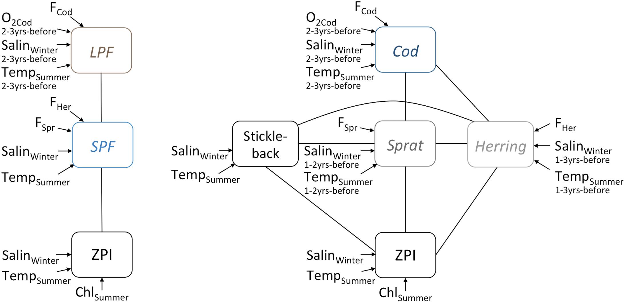
Figure 2. Network architecture, illustrating potential drivers and pressures evaluated for their impact on indicators, including relationships between indicators that may arise due to species interactions. LPF, Large Predatory Fish; SPF, Small Prey Fish; ZPI, zooplankton-based indicator (one of Total Zooplankton Abundance, Mean Size or Ratio of cladocerans to copepods); F, fishing mortality (species-specific), Chl_Summer, chlorophyll a during summer, Temp_Summer, summer sea surface temperature, Salin_Winter, winter deep-water salinity (the latter two with species-specific time-lags).

Climate-related pressures (Temp_Summer, Salin_Winter, O_2Cod) were viewed as non-manageable pressures at the regional level, as future climate trajectories will largely depend on decisions made at other scales. Fisheries and eutrophication were considered manageable, as management decisions are made within regional governance structures or by national bodies incorporating regional agreements or plans (e.g., HELCOM, 2013a). O_2Cod is an effect of both large-scale climate variations influencing water inflows from the North Sea to the Baltic Sea and regional eutrophication, and as such is partly related to Chl_Summer and was not included as pressure in the future predictions.

Statistical Modeling

Our statistical modeling approach included three steps (Figure 1): (1) Fitting statistical models for each indicator and basin, including potential pressures and links to other indicators identified a priori based on existing knowledge and plausible relationships (Figure 2). (2) Building indicator networks by combining the relationships identified in 1. (3) Simulating the effects of different management scenarios under climate change on the indicators using the statistical indicator networks. Statistical modeling was carried out in R 3.0.2 and 3.2.4 (R Core Team, 2016).

Development and Selection of Indicator Models

The statistical models for individual indicators were Generalized Additive Models (GAMs) (Wood, 2006) or their threshold formulation (tGAMs) (Ciannelli et al., 2004), developed using the mgcv library (Wood, 2006).

A variance inflation factor (VIF) test was performed on each set of potential covariates (pressures and links to other indicators) to detect and avoid issues of multicollinearity (Zuur et al., 2010). We excluded one variable at a time (the one with the highest VIF) when any VIF > 3 until we had reduced sets of covariates with all VIF ≤ 3. All a priori identified covariates were thus tested for effects in at least one set.

We did not model autoregressive effects but included only external pressures as explanatory variables, as our focus was not on autoregressive processes and several indicators were aggregated across species or groups. No interactions between explanatory variables were evaluated due to the size of the datasets and tGAMs representing a form of interaction between covariates.

Selecting GAMs

All possible additive combinations of covariates were compared for each individual indicator in the GAM analyses. GAM comparisons were made based on Generalized Validation Criterion (GCV; Wood, 2006), where a lower GCV means a more parsimonious model. We checked model diagnostics of candidate models (see Supplementary Information: Appendix I), and ultimately selected the statistically best model that had sensible ecological effects (i.e., not contradicting existing ecological knowledge, for example a positive direct effect of higher fishing mortality or of a competitor).

Selecting tGAMs

For tGAMs, we constructed starting models, using as large as possible sets of covariates, taking into account VIF results and ensuring that the model degrees of freedom did not exceed the length of the time series. Models including size-based FI had simpler structure (Figure 2), making it feasible to try all potential pressures and use threshold variables defined a priori. Models including abundance-based fish indicators had a higher number of potential trophic links and threshold variables, so we used the results of the GAM analysis and results from single-pressure analyses carried out by Otto et al. (2018) to inform choice of covariates and threshold variables (see details in Supplementary Information: Appendix I).

Each starting tGAM was reduced in a step-wise manner, by excluding the explanatory variable with highest p-value until all explanatory variables had p < 0.05, after which model GCV was minimized to identify the most parsimonious model. We examined the effects of explanatory variables above and below the threshold, confirming that these indeed were qualitatively different. If not, the model was simplified by removing the threshold effect on that explanatory variable until variables with thresholds had qualitatively different dynamics. After examination of model diagnostics, we calculated the genuine cross validation score (genuine CV; Ciannelli et al., 2004) of the tGAM, which equals the average squared leave-one-out prediction errors and accounts for the grid search needed to find the value of the threshold. This was compared to the genuine CV of the corresponding GAM, i.e., with the same model structure except for the threshold. If the tGAM had a lower genuine CV, it was added to the list of candidate tGAMs. After completing this process with all starting models, we compared the candidate tGAMs using GCV and examining the ecological relationships. As for GAMs, we selected the statistically best tGAM that had sensible ecological effects.

Selecting final model

If the selected tGAM had a higher genuine CV than its corresponding GAM, i.e., being a less suitable model, a GAM would be the best model for the indicator and we picked the selected GAM as the final model. If the selected tGAM had a lower genuine CV than its corresponding GAM, i.e., being a more suitable model, the selected tGAM was picked when the covariates in the models were the same as the models’ genuine CV are comparable in this situation. If the selected GAM and tGAM differed in their covariates we could not use the genuine CV to choose the final model. Instead, we picked the model with the most simple structure (a GAM in all cases).

We did not find statistically sound models with reasonable ecological effects among models for the Cod and LPF indicators in the Gotland Basin, or for Stickleback in the Bornholm Basin. In these cases, the observed indicator time series was only used as a covariate when relevant for the indicator networks.

Construction of Indicator Networks

The selected indicator models were coupled into an indicator network, where the dynamics were driven by the external covariates (environmental and climate variables, fishing) and trophic interactions as identified by the individual indicator models. We used the predicted value of an indicator to feed into any other model component where it had an effect, until all indicators in the network had been predicted. Noise, in the form of resampled residuals from the individual indicator models, was added to test the robustness of predictions and generate confidence intervals.

Indicators at two trophic levels simultaneously affected each other in some of the networks (Figures 3, 4). In this case, we started the coupling by adding the observed value of one indicator into the model predicting the other, then using the modeled value to predict the first indicator and repeating until convergence was reached.

FIGURE 3

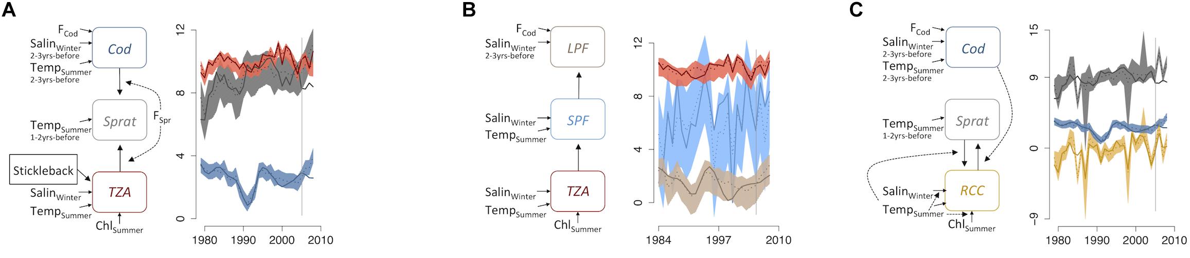
Figure 3. Indicator networks in the Bornholm Basin in the Baltic Sea. (A) Abundance-based zooplankton indicator (ZPI) and abundance-based fish indicators (FI), (B) Abundance-based ZPI and size-based FI, and (C) ratio-based ZPI and abundance-based FI. Left side of each panel shows model structure, where solid lines illustrate direct effects and dotted lines illustrate threshold variables between indicators and/or external forcing variables. The right side shows the time series plots, where solid lines illustrate original data and dotted lines illustrate the mean predicted annual values from coupled models (with 95% confidence intervals). TZA, total zooplankton abundance; MS, zooplankton mean size; RCC, abundance ratio of cladocerans to copepods (excluding nauplii); SPF, small prey fish; LPF, large predatory fish; F, fishing mortality (species-specific), Chl_Summer, chlorophyll a during summer; Temp_Summer, summer sea surface temperature; Salin_Winter, winter deep-water salinity (the latter two with species-specific time-lags).

FIGURE 4

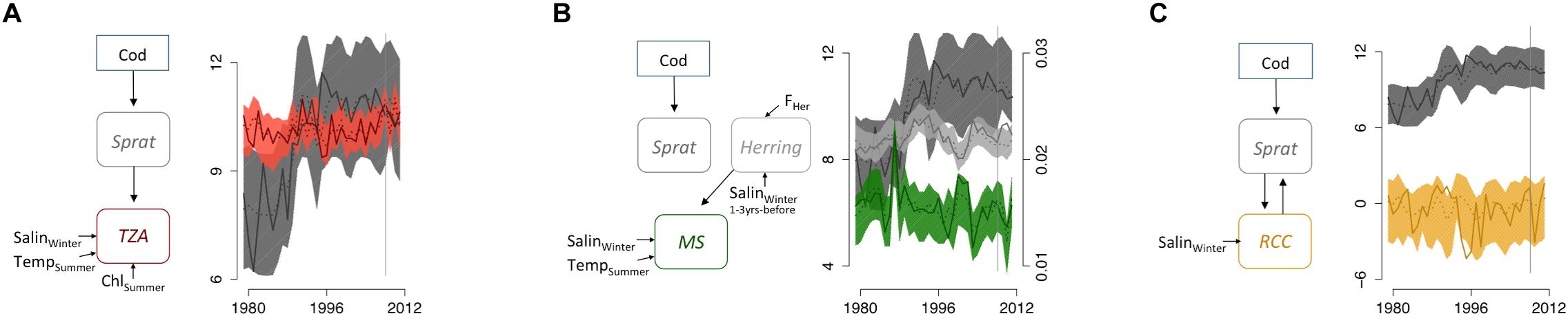
Figure 4. Indicator networks in the Gotland Basin in the Baltic Sea. (A) Abundance-based zooplankton indicator (ZPI) and abundance-based fish indicators (FI), (B) Size-based ZPI and abundance-based FI, and (C) ratio-based ZPI and abundance-based FI. Left side of each panel shows model structure, where solid lines illustrate direct effects and dotted lines illustrate threshold variables between indicators and/or external forcing variables. The right side shows the time series plots, where solid lines illustrate original data and dotted lines illustrate the mean predicted annual values from coupled models (with 95% confidence intervals). For abbreviations, see Figure 3.

Lastly, we validated the indicator networks by predicting the last 3 years of the time series – that were not used for fitting individual indicator models – and compared predicted versus observed values. Poor performance during the validation period did, however, not disqualify networks from simulations of future scenarios, as we were interested in seeing if robustness of relationships affected conclusions.

Simulations of Management Alternatives and Climate Change

Future scenarios for regionally manageable pressures covered years 2012–2040 and included high and low levels of fisheries exploitation for cod and clupeids and three levels of nutrient loads: reductions following the Baltic Sea Action Plan (HELCOM, 2013a), reference levels (PLC 5.5, HELCOM, 2015) and increase due to intensified agriculture in the catchment area. A realistic climate change scenario, corresponding to SRES emission scenario A1B, was simulated by two global models, HadCM3 and ECHAM5, to illustrate uncertainty (Gordon et al., 2000; Roeckner et al., 2006). Regionally downscaled climate variables from the two climate projections and nutrient load scenarios were modeled by the coupled physical-biogeochemical model BALTSEM (Gustafsson, 2003; Gustafsson et al., 2012) to simulate these future pressures at the basin scale. BALTSEM runs thereby generated simulated time series of sea surface temperature, deep-water salinity and of chlorophyll α subsequently used in our scenario simulations (Supplementary Figure S2). Sensible models for piscivorous FI in the Gotland Basin were not identified, and we instead constructed time series to investigate impacts of a range of future Cod levels on other indicators. Details about the climate projections, scenarios for nutrient load and fisheries exploitation as well as the BALTSEM model and Cod future time series are found in Supplementary Information: Appendix I.

The quantitative relationships of the networks and the scenario data were used to project the indicators by running a thousand Monte Carlo simulations for each indicator and year. Noise was added in each simulation by sampling from the residuals (from model component runs on observed data). We calculated a mean and 95% confidence intervals based on bootstrapping of estimated values for each indicator and year.

Effect sizes and interactions between pressures under the scenarios were evaluated by running multi-factorial ANOVA or Generalized Least Squares (GLS) models. Since simulated time series tend to show less stochasticity and higher autocorrelation GLS were applied when temporal autocorrelation was detected, using auto-regressive error structures of order 1 or 2, depending on the detected autocorrelation (Pinheiro and Bates, 2000). We started with a full model, including higher-order interaction terms, and applied a backward-selection based on Akaike’s Information Criterion (AIC).

Results

Individual Indicator Models

In the first step (Figure 1), sensible models were found for 19 of 22 food-web indicators (Supplementary Table S1 and Supplementary Figure S3). GAMs were often sufficient to capture observed variation in the indicators, where non-linear relationships were present in about half of all responses (Supplementary Table S1). Threshold formulations (tGAMs) performed better in a few cases, mostly related to Sprat dynamics (Supplementary Table S1).

Indicator Networks

The majority of the individual indicator models suggested links between indicators (Supplementary Table S1), making it possible to couple individual indicator models to each other into eight indicator networks (Table 1 and Figures 3, 4). All networks reproduced the overall pattern of observed indicator time series used for fitting, but did not always capture temporal variation (Figures 3, 4 and Supplementary Figure S4). Observations during the time periods used for validation were replicated well by some networks (e.g., Figure 3B), but other networks had worse performance when predicting data points not previously considered in the individual models (e.g., Figure 3C).

TABLE 1

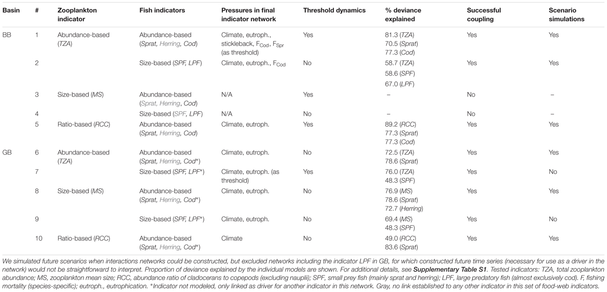
Table 1. Summary of model selection and coupling of individual indicator model components into indicator networks for the Bornholm (BB) and Gotland Basins (GB) in the Baltic Sea.

The complexity of indicator networks varied. For example, the network of size-based ZPI and FI in the Gotland Basin, had low complexity; with unidirectional trophic control and summer sea surface temperature being the only external pressure (Supplementary Figure S5B). Other models included multiple pressures, threshold effects and mixed trophic control (e.g., abundance ZPI and FI models in the Bornholm Basin, Figure 3A).

Links between indicators representing different trophic levels were key explanatory factors. On the other hand, links between indicators at the same tropic level – corresponding to competition, which we investigated for planktivore-based FI – were not detected (Supplementary Table S1). Sprat and the size-based SPF were often linked to ZPI as well as piscivorous FI, making tri-trophic indicator networks the most common configuration (Figures 3, 4). There was only one case of a link between Herring and another indicator. The piscivorous FI Cod and LPF always exerted a top-down control on planktivore-based FI, except in one interaction network (Figure 3B). Direction of coupling between ZPI and planktivore-based FI differed between networks, and bidirectional linkages were found as well (Figures 3, 4 and Supplementary Figure S5). Five of the indicator networks included a direct effect of a manageable pressure on one indicator; which in turn had a relationship with another indicator (Figures 3, 4B and Supplementary Figure S5A), suggesting that trophic interactions could introduce indirect links between pressures and indicators. The same type of pattern involving climate variables existed in five networks.

Impacts of Regionally Manageable Pressures

A few key pressure variables had similar effects across the different indicator networks. Chlorophyll a – as a proxy for eutrophication – emerged as a central pressure variable in the Bornholm Basin where we found significant relationships with all three types of ZPI (Supplementary Table S1). In the Gotland Basin, only TZA responded to this pressure (Supplementary Table S1). Indicators responding to fishing pressure variables were relatively fewer. In the Bornholm Basin significant effects of F_Cod on Cod and LPF (direct effect, Supplementary Table S1) were detected, which indicator network structure suggested would cascade onto Sprat (as an indirect effect, Figures 3A,B). F_Her affected Herring in the Gotland Basin (Figure 4B). Ecologically meaningful (i.e., negative) effects of F_Spr on sprat were not detectable.

The scenario simulations highlighted indirect and cascading effects of management measures suggested by the structures of the indicator networks (Tables 1, 2 and Figures 5, 6). While the network structures suggested that management measures may have indirect effects on quite many indicators, the simulations revealed that detectable indirect effects involved fewer indicators. In the Bornholm Basin, we found significant indirect effects of nutrient input on Sprat and SPF values, two planktivore FI (see Supplementary Table S2). Both indicators showed lower values under decreased nutrient input (Figure 5B and Supplementary Figures S6, S7), suggesting a strong bottom-up control of these interlinked indicators. However, when accounting for the coupling of Sprat to the ZPI RCC, the nutrient effect was reversed (Figure 5C and Supplementary Figure S8). In the Gotland Basin, the size-based ZPI MS was affected by a top-down effect from clupeid fisheries, acting via Herring (Figures 4B, 6B). While this effect was significant, it had a weak response (Table 2).

TABLE 2

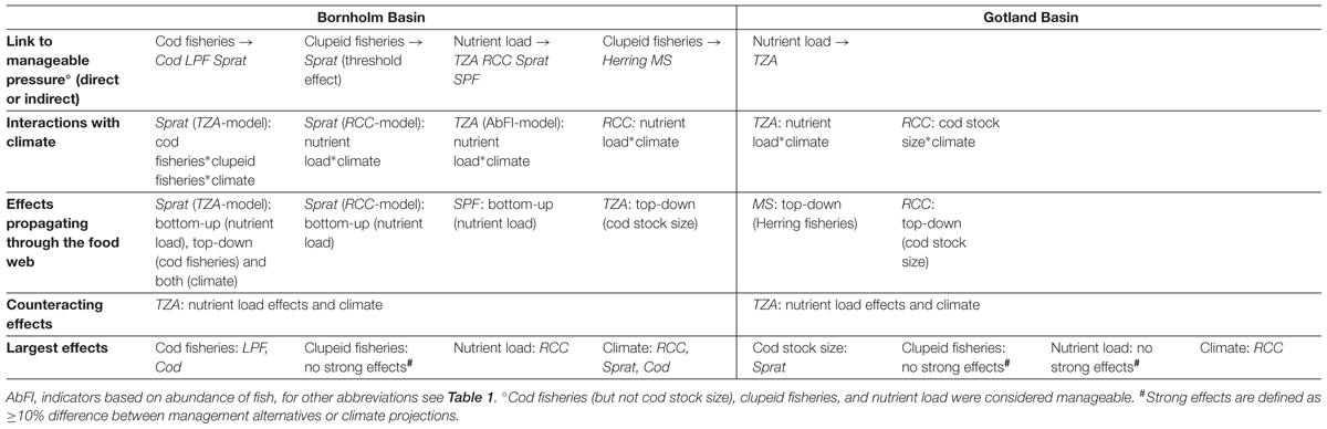
Table 2. Structural links, and effects of scenarios of eutrophication, fisheries, and climate, on proposed food-web indicators for two basins in the central Baltic Sea simulated for the years 2012–2040, based on statistical indicator networks.

FIGURE 5

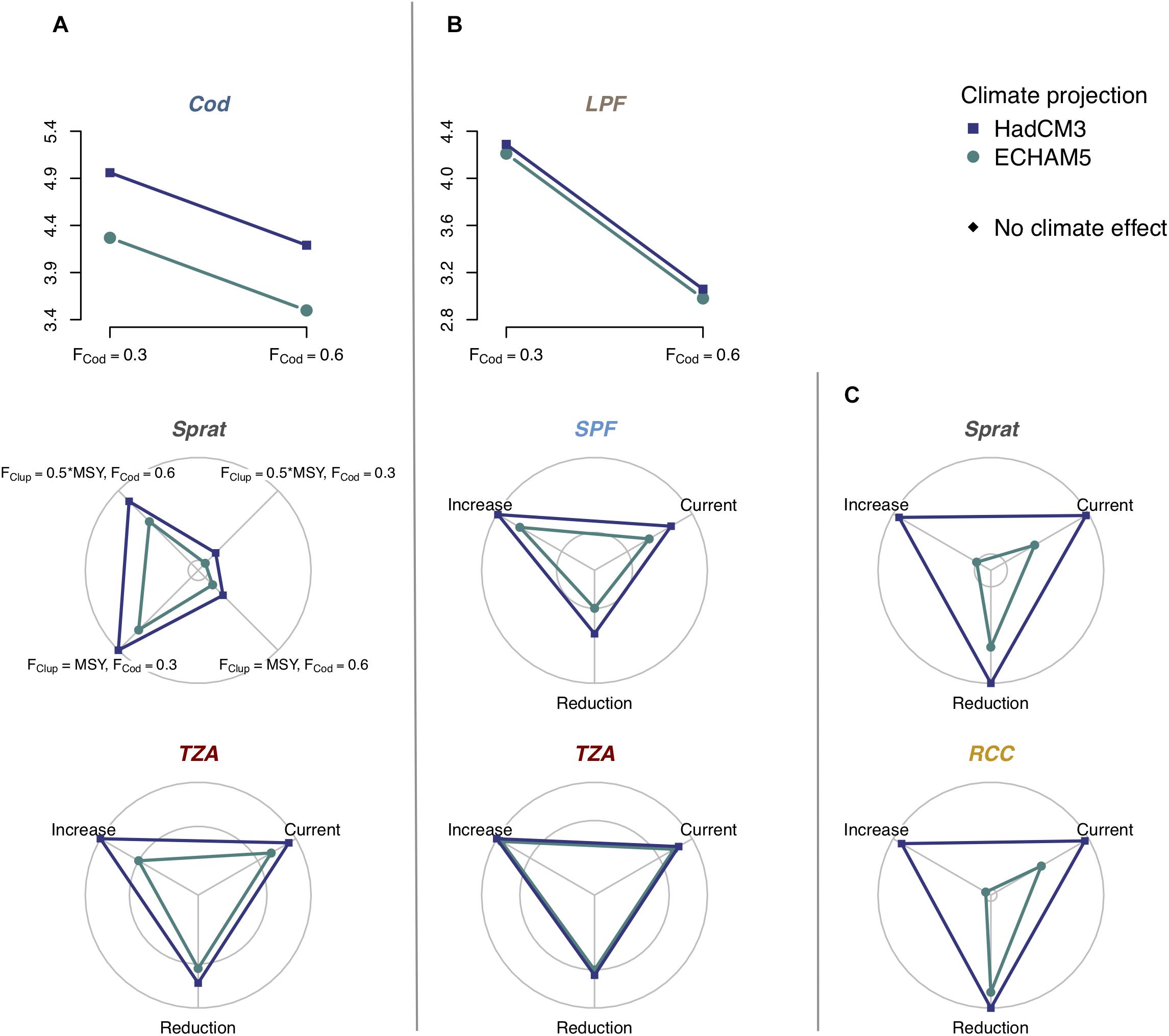
Figure 5. Influence of climate change on indicator responses to management scenarios, including interactions between climate and management measures and additive effects of climate. The line and radar charts show significant differences between two or more scenarios, detected by GLS analysis, in the Bornholm Basin, where letters (A–C) correspond to the models shown in Figure 3. Blue represents climate projections from the HadCM3 model and green represents projections from the ECHAM5 model. Black indicates no effect of climate on the indicator. Each axis in the radar charts represents one fishery, cod stock or eutrophication scenario. The outer ring in radar charts correspond to the maximum effect size, the inner ring corresponds to minimum effect size and the center 90% of the minimum effect size. The differences between scenarios are thus small, when the two rings are close to each other. Interactions between climate and manageable pressures were found for the lower trophic levels, but not the piscivorous level where effects were additive. Future climate conditions had consistent effects across all indicators in the Bornholm Basin. For clear illustration of the effects of climate, we only show the interaction between climate and one pressure for Sprat in (A), but effects of a second pressure, not interacting with climate, are not shown. Supplementary Tables S1, S2 and Supplementary Figures S5–S11 present complete results of the analysis. TZA, total zooplankton abundance; MS, zooplankton mean size; RCC, abundance ratio of cladocerans to copepods (excluding nauplii); SPF, small prey fish; LPF, large predatory fish; F, fishing mortality (species-specific, F_Clup refers to the clupeids sprat and herring); MSY, maximum sustainable yield; Chl_Summer, chlorophyll a during summer; Temp_Summer, summer sea surface temperature; Salin_Winter, winter deep-water salinity (the latter two with species-specific time-lags).

FIGURE 6

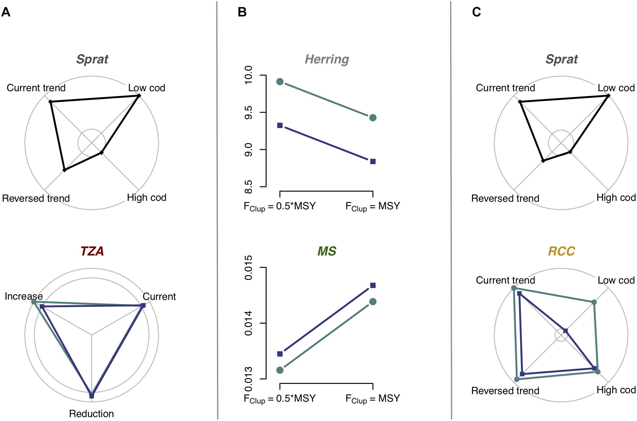
Figure 6. Influence of climate change on indicator responses to management scenarios, including interactions between climate and management measures and additive effects of climate. The line and radar charts show significant differences between two or more scenarios, detected by GLS analysis, in the Gotland Basin, where letters (A–C) correspond to the models shown in Figure 4. For abbreviations as well as interpretation of radial axes and colors, see Figure 5. Effects on the piscivorous trophic level could not be assessed in the Gotland Basin. Two (A,C) out of three indicator networks here showed interactions between scenarios. Future climate conditions had inconsistent effects in the Gotland Basin. For clear illustration of the effects of climate, we only show the interaction between climate and one pressure for TZA in (A), but effects of a second pressure, not interacting with climate, are not shown. Supplementary Tables S1, S2 and Supplementary Figures S5–S11 present complete results of the analysis.

No ecologically meaningful model was identified for Cod in the Gotland Basin, but the indicator networks showed a top-down effect of Cod on Sprat, in turn affecting the ZPI TZA as well as RCC, in their respective networks (Figures 4A,C). Any pressure acting on Cod could thereby have cascading effects on lower trophic level indicators in the Gotland Basin.

Interactions between regionally manageable pressures, i.e., an indicator responding to two or more pressures, were rather sparse: these were only found for Sprat in the coupled model of abundance ZPI and FI in the Bornholm Basin. Here, we found a cascading effect of cod fisheries, which was modulated by the threshold effect of clupeid fishing mortality: The positive effect of higher cod fishing pressure, leading to lower cod stock size and hence predation pressure for sprat, occurred only under reduced clupeid fisheries (i.e., at 0.5^∗F_MSY) and was even reversed when increasing clupeid fishing pressure to F_MSY (Figure 5A and Supplementary Figure S6). Other than this interaction, the simulations suggested that the structural links between indicators across trophic levels did not result in detectable trade-offs between management objectives, for the pressures and indicators we studied.

Role of Climate and Interaction With Management Measures

Future climate was projected to have marked impacts on the performance of indicators and indicator relationships to pressures (Figures 5, 6). In the Bornholm Basin indicator values were overall higher under the HadCM3 model (projections resulted in overall higher temperatures, higher salinity and lower Chl a than in the projections from ECHAM5, see Supplementary Figure S2). The effect was small on TZA and LPF, but there were strong effects on all other indicators (Supplementary Table S2 and Figure 5). The two climate projections had less pronounced impacts on the results for the Gotland Basin (Supplementary Table S3). Effects were found on all three ZPI and on Herring. In this basin, there was no consistent difference between climate models with respect to indicator values (Figure 6).

Importantly, we found a striking pattern in terms of how climate modified responses to other pressures (Table 2 and Figures 5, 6): the climate variables interacted almost exclusively with the nutrient scenarios. Climate variables either modulated the magnitude of the indicators’ response to nutrient load reductions, as found for Sprat (Figure 5C and Supplementary Figure S8) and the ratio ZPI RCC (Figure 5C and Supplementary Figure S8), or counteracted the nutrient load effect on the abundance-based ZPI TZA (Figure 5A and Supplementary Figure S6; with a very small effect: Figure 4A and Supplementary Figure S9).

Discussion

Understanding Indicator Responses Under Cumulative Pressure Regimes

A key element needed for traditional management to evolve into agile EBM is an holistic approach that recognizes the full array of interactions between single species and ecosystem components (Slocombe, 1993). Yet, when it comes to developing indicators as tools for status assessment of marine food webs and management strategy evaluations, such an integrated approach is often ignored for wider ranges of ecosystem- and resource-use objectives than fisheries (Sainsbury et al., 2000). Independent of whether indicators are based on single species, species groups or aggregated metric such as mean community size (Teixeira et al., 2014), they will integrate system-specific interactions and environmental effects (Torres et al., 2017). To ensure accurate interpretation of indicator responses to manageable as well as unmanageable pressures, and to account for cascading effects of management measures, potentially resulting in conflicting management objectives, it is essential to disentangle and quantify such interactions. An approach that integrates several pressures and multiple indicators representing different trophic guilds is thus needed when developing food-web indicators. In our case study, most long-term observed trends of indicators were explained by the combined effect of system-internal variables, i.e., other food-web indicators, and external variables relating to fishing pressure, eutrophication or climate. These results were also independent of the type of indicator (single species-based or aggregated) or trophic level. We did, however, find that indicator responses differed between the Baltic Sea basins.

Appropriate Spatial Scales for Indicators and Evaluations

There was substantial variation in indicator responses to pressures, but in some cases clear patterns emerged. In one basin (Bornholm), responses to climate were consistent across all indicators despite substantial differences in the performance of indicator networks. In the other basin (Gotland), responses to climate were not consistent while differences in performance between indicator networks were smaller. These types of results confirm the need to carry out system-specific or spatially explicit performance evaluations (Shin et al., 2018).

However, in the Gotland basin, we struggled to identify ecologically sensible models for the two indicators of the apex predator guild, Cod and LPF. This could be due to missing an important covariate or a mismatch between data (indicator or covariate) and spatio-temporal dynamics (Bartolino et al., 2017). Fish-based indicators (for the species studied herein) could potentially be more meaningful if they instead are estimated at the broader central Baltic Sea level. The most abundant fish species in the Baltic Sea – which the indicators are based upon – move seasonally and have occupied different ranges over time, mainly regulated by density-dependence (Casini et al., 2011; Bartolino et al., 2017). Our results did neither reveal interactions between climate and fishing pressure as found in previous studies (Gårdmark et al., 2013). This may be an artifact of the different spatial scales (fishing mortality estimates were only available for the entire Baltic Sea and thus did not constitute basin-specific covariates).

These results suggest that alternating between region-wide and basin-specific application of indicators may therefore be required for comprehensive sets of indicators under cumulative pressure regimes.

Advantages and Challenges With the Indicator Networks

Our indicator networks were based on statistical models (GAMs and tGAMs), enabling us to test for non-linear effects and even threshold effects of pressures, i.e., if ecosystem dynamics above and below the threshold value are qualitatively different. Threshold dynamics in marine ecosystems have been observed in many different systems, for example coral reefs (Knowlton, 1992) and pelagic food webs (Conversi et al., 2015). However, they are rarely accounted for in EBM indicator evaluations, perhaps due to quantitative validation schemes only being recently developed (Queirós et al., 2016; Otto et al., 2018). Non-linear effects were relatively common in our indicator networks, while threshold effects were more rare. Threshold dynamics and different ecosystem configurations have been identified in the Baltic Sea (Casini et al., 2009), so it was not surprising that a few networks functioned similarly. As a consequence of threshold dynamics some indicator responses may be challenging to connect to pressures, if not accounted for. For example, it was not possible to adequately model the Ratio of cladocerans to copepods indicator in one basin using GAMs only, but when incorporating threshold dynamics a well-performing model was found. However, sometimes responses are difficult to interpret even after threshold dynamics have been identified, as exemplified by the intricate effects of cod and clupeid fisheries on the Sprat indicator in one of our indicator networks (see Figure 5A and Supplementary Figure S6). Such results may appear discouraging and could rise from spurious relationships between the particular monitoring time series used, but without this type of quantitative approach, anticipation of these relationships appears close to impossible.

A few of the indicator networks had worse performance during the validation period than the period used for fitting individual indicator models, suggesting that these relationships were not very robust (i.e., non-stationary). The insights from our study – regarding substantial impacts of climate on the indicators as well as abundant links between indicators representing different trophic levels – rest, however, on the results from several indicator networks.

The indicator network approach was well suited to identify broad-scale factors affecting interpretation of indicator values, such as climate, and the presence of trophic interactions modifying indicator interpretation as well as feasibility of achieving multiple objectives. As any quantitative approach it is sensitive to availability and quality of data. The lack of long-term datasets on key ecosystem components may impede application in data-poor systems. The Baltic Sea is relatively data-rich and we were able to include threshold dynamics, but not other types of interactions between pressures, as that would have led to over-fitting of models. However, as a minimum, statistical modeling and indicator networks provide information that data availability or quality may be insufficient. For identifying operational food-web indicators, the ability to examine relationships and responses at the scale of ecosystem assessments, or finer, constitute a major improvement over expert opinion and panaceas for all marine ecosystems.

The challenges highlighted by relatively data-hungry and potentially complex underlying models emphasize at the same time the main advantage of the indicator networks: the ability to test for multiple pressure effects and indicator linkages simultaneously, which may be essential as some relationships may only be revealed by modeling all time series jointly (Torres et al., 2017, this study: Figure 3 and Supplementary Information: Appendix II), and without an a priori specification of the shape of relationships. When relationships between indicators representing different trophic levels or guilds have been identified, the indicator networks enable further investigation of how effects of single or multiple management measures may propagate through the food web.

Another potential constraint of our presented approach can be time-consuming analyses related to the complexity of the food web and the number of indicators to test. The GAM/tGAM coupling approach to build the network relies on individual models for each indicator. With increasing food web complexity, there are more models to fit and couple, the more time-consuming this approach becomes.

Trophic Interactions and Achievable Management Targets

Relationships across trophic levels or between guilds may have strong implications for management measures, ranging from effectiveness of single measures to human-induced trophic cascades and conflicts between management objectives (Estes et al., 2011; Reilly et al., 2013).

Our example suggested bottom-up control of planktivorous FI in one basin and top-down control on most indicators in the other basin. This pattern has strong implications for management strategies. Interpreted together with the scenario simulations, the results point to that nutrient load reductions (as planned in the region, HELCOM, 2013a) may have limited effectiveness in one area (Gotland Basin, where top-down control was more prevalent) while these measures are likely to impact even the state of the indicators at intermediate trophic levels in the other area (Bornholm Basin, with bottom-up control). The net effect of management measures is difficult to predict with simple modeling approaches, as overall effects of multiple stressors may be additive, synergistic or antagonistic depending on the response level (population or community), trophic level as well as the stressors involved (Crain et al., 2008). This applies especially when different pressures are targeted simultaneously, as in our scenarios and many real cases. The net effect may, however, be estimated through simulations, after indicator relationships, across trophic levels or between individual species, have been quantified. Such quantification of propagating effects is essential for determining if trade-offs between management objectives are likely to occur.

Potential Trade-Offs Between Management Objectives

A profound challenge in management governed by policies with multiple objectives is to account for trade-offs that can exist between individual management objectives (McClanahan et al., 2011). Ambitions to eliminate effects of eutrophication may have negative effects on biodiversity, for example: the abundance of benthic-feeding ducks declines as fewer, smaller and less-nutritious mussels are available to feed upon, concurrent with lowered nutrient levels in the ecosystem (Laursen and Moller, 2014). Trade-off directions in multi-objective EBM are tightly linked to the direction of trophic control in the ecosystem, which is not necessarily static or unidirectional (Lynam et al., 2017). During top-down forcing, management measures targeting indicators representing higher trophic levels, e.g., reductions in fishing pressure on piscivorous fish, are also likely to influence indicators representing a lower level of the food web, such as forage fish. Such effects on fish-based indicators were also detected in our case study (Supplementary Tables S2, S3 and Figure 5). Trade-offs between objectives and difficulties defining targets and thresholds may emerge already when two trophic levels are involved. This includes cases when there should be no adverse effects on balances between trophic guilds or on population characteristics of fished stocks (see e.g., criteria for good environmental status in EU decision 2017/848).

Mixed trophic control may lead to substantial conflicts between objectives. If there are other forage fish predators, in such an ecosystem as above, that instead are food-limited, indicators of their status will illustrate adverse effects of the implemented measures for piscivorous fish. Reilly et al. (2013) describe how reduced fishing pressures on North Sea haddock and whiting are likely to result in increased abundance of these species, followed by higher predation pressure on sandeels reducing their abundance, with potentially detrimental impacts on kittiwake populations. This situation represents incompatible sets of objectives as the indicators and their target levels currently are defined (Reilly et al., 2013). We did not find indications of marked trade-offs between objectives in our case study, but our models included relatively few species. They did for example not include other forage fish predators, e.g., auks or seals, which potentially could give different results. When there is a risk of conflicts between objectives, multiple covariate models that couple several indicators, such as our indicator networks, have the advantage to allow for multidirectional trophic control and quantification of links between indicators representing different trophic levels, or guilds. Such quantification enables management bodies to anticipate trade-offs as well as to adjust targets and action thresholds to accommodate them, once priorities between the conflicting objectives have been decided politically (Martin et al., 2009).

Management Under Modulating Effects of Climate Change

The influence of current and future climate is essential to consider when evaluating management options and setting thresholds, as large-scale environmental pressures may provide critical context for decisions in EBM, despite not being directly controllable in the short term (Samhouri et al., 2017). Our simulations depict this situation and illustrate strong modulating effects of climate change on the food-web indicators, and hence, on effects of other management measures. Both temperature and salinity were linked to the observed long-term development of most indicators we tested. Most importantly, future climate magnified and in other cases interfered with effects of management measures in our simulations. This is expected given the links between indicators representing trophic levels in the indicator networks. In our example, interactions between climate and nutrient load reductions were suggested, affecting the development of zooplankton-based indicators across regions. For the aggregated indicator TZA, the results suggest that this interaction has even the potential to counteract effects of eutrophication mitigation measures. This implies that the meaning of the indicator, for evaluation of management options, evolves with a changing climate.

Adaptive approaches appear central to handle such effects of climate change, as explicit recognition of the uncertainty and unpredictability is needed, along with a structured process for management response. A key feature of adaptive management is the ability to respond to environmental feedback through monitoring, (re)-assessments and new management options (Allen et al., 2011; Williams, 2011). Quantification of links between multiple pressures and indicators across interacting trophic levels, followed by simulations including climate change, is central for management strategy evaluations and management design. This enables identifying potential trade-offs and dependencies between manageable and unmanageable pressures. To learn about current meaning of indicators, evaluation and validation of indicators need to be done in an iterative manner. More frequent evaluations, using approaches like our indicator networks that also allow for threshold-shaped relationships to pressures and each other, of the present and projected near-term climate development, could lead to regular re-adjustments of indicator target and threshold values. Such processes could be one way to apprehend the uncertainty related to potentially modulating effects of climate, or other large-scale environmental pressures (Samhouri et al., 2017). We foresee that this kind of flexible strategies make a set of indicators operational long-term and provide a route-map to navigate impacts of climate change. Incorporation of these approaches in EBM is essential if we want to ensure human well-being while preserving our ocean ecosystems in an increasingly uncertain future.

Author Contributions

AG and SO conceived the original idea. MK, TB, and SO designed the research. MC and SO prepared the data. MK and SO analyzed the data. MK led the writing with contributions from TB, MC, MT, AG and SO.

Funding

This study is a contribution to the project ‘Ecosystem-based approach for developing and testing pelagic food-web indicators’ financially supported by the Swedish Environmental Protection Agency (Grant No. 20704801). The scenario work was additionally supported by the Swedish Agency for Marine and Water Management (Grant No. 1862-16). MC and TB were also partially financed by the BONUS INSPIRE project supported by BONUS (Art 185), funded jointly by EU and the Swedish Research Council FORMAS, AG was partially financed by a Swedish Research Council FORMAS (Grant No. 217-2013-1315). TB and SO were also partially financed by the BONUS BLUEWEBS project supported by BONUS (Art 185).

Conflict of Interest Statement

The authors declare that the research was conducted in the absence of any commercial or financial relationships that could be construed as a potential conflict of interest.

Acknowledgments

We would like to thank colleagues from the Department of Fish Resources Research, Institute of Food Safety, Animal Health and Environment (BIOR) in Latvia, the Finnish Environment Institute (SYKE), the Leibniz Institute for Baltic Sea Research Warnemünde (IOW) in Germany, and the Swedish University of Agricultural Sciences (SLU) for maintaining these extensive long-term monitoring programs. Threshold functions for tGAMs were supplied by Lorenzo Ciannelli and Kung-Sik Chan. BALTSEM runs were generated as part of the BONUS ECOSUPPORT project and provided by the Baltic Nest Institute, Stockholm University.

Supplementary Material

The Supplementary Material for this article can be found online at: https://www.frontiersin.org/articles/10.3389/fmars.2019.00249/full#supplementary-material

References

Allen, C. R., Fontaine, J. J., Pope, K. L., and Garmestani, A. S. (2011). Adaptive management for a turbulent future. J. Environ. Manag. 92, 1339–1345. doi: 10.1016/j.jenvman.2010.11.019

PubMed Abstract | CrossRef Full Text | Google Scholar

Bartolino, V., Tian, H., Bergström, U., Jounela, P., Aro, E., Dieterich, C., et al. (2017). Spatio-temporal dynamics of a fish predator: density-dependent and hydrographic effects on Baltic Sea cod population. PLoS One 12:e0172004. doi: 10.1371/journal.pone.0172004

PubMed Abstract | CrossRef Full Text | Google Scholar

Blenckner, T., Llope, M., Mollmann, C., Voss, R., Quaas, M. F., Casini, M., et al. (2015). Climate and fishing steer ecosystem regeneration to uncertain economic futures. Proc. R. Soc. B 282:20142809. doi: 10.1098/rspb.2014.2809

PubMed Abstract | CrossRef Full Text | Google Scholar

Casini, M., Hjelm, J., Molinero, J. C., Lövgren, J., Cardinale, M., Bartolino, V., et al. (2009). Trophic cascades promote threshold-like shifts in pelagic marine ecosystems. Proc. Natl. Acad. Sci. U.S.A. 106, 197–202. doi: 10.1073/pnas.0806649105

PubMed Abstract | CrossRef Full Text | Google Scholar

Casini, M., Kornilovs, G., Cardinale, M., Mollmann, C., Grygiel, W., Jonsson, P., et al. (2011). Spatial and temporal density dependence regulates the condition of central Baltic Sea clupeids: compelling evidence using an extensive international acoustic survey. Popul. Ecol. 53, 511–523. doi: 10.1007/s10144-011-0269-2

CrossRef Full Text | Google Scholar

Casini, M., Lovgren, J., Hjelm, J., Cardinale, M., Molinero, J. C., and Kornilovs, G. (2008). Multi-level trophic cascades in a heavily exploited open marine ecosystem. Proc. R. Soc. B 275, 1793–1801. doi: 10.1098/rspb.2007.1752

PubMed Abstract | CrossRef Full Text | Google Scholar

Casini, M., Tian, H., Hansson, M., Grygiel, W., Strods, G., Statkus, R., et al. (2019). Spatio-temporal dynamics and behavioural ecology of a “demersal” fish population as detected using research suvey pelagic trawl catches: the Eastern Baltic Sea cod (Gadus morhua). ICES J. Mar. Sci. doi: 10.1093/icesjms/fsz016

CrossRef Full Text

Ciannelli, L., Chan, K. S., Bailey, K. M., and Stenseth, N. C. (2004). Nonadditive effects of the environment on the survival of a large marine fish population. Ecology 85, 3418–3427. doi: 10.1890/03-0755

PubMed Abstract | CrossRef Full Text | Google Scholar

Cloern, J. E., Abreu, P. C., Carstensen, J., Chauvaud, L., Elmgren, R., Grall, J., et al. (2016). Human activities and climate variability drive fast-paced change across the world’s estuarine–coastal ecosystems. Glob. Chang. Biol. 22, 513–529. doi: 10.1111/gcb.13059

PubMed Abstract | CrossRef Full Text | Google Scholar

Conversi, A., Dakos, V., Gårdmark, A., Ling, S., Folke, C., Mumby, P. J., et al. (2015). A holistic view of marine regime shifts. Philos. Trans. R. Soc. B 370:20130279. doi: 10.1098/rstb.2013.0279

CrossRef Full Text | Google Scholar

Crain, C. M., Kroeker, K., and Halpern, B. S. (2008). Interactive and cumulative effects of multiple human stressors in marine systems. Ecol. Lett. 11, 1304–1315. doi: 10.1111/j.1461-0248.2008.01253.x

PubMed Abstract | CrossRef Full Text | Google Scholar

Dayton, P. K., Thrush, S. F., Agardy, M. T., and Hofman, R. J. (1995). Environmental effects of marine fishing. Aqua. Cons. Mar. Freshw. Ecosys. 5, 205–232. doi: 10.1002/aqc.3270050305

CrossRef Full Text | Google Scholar

Estes, J. A., Terborgh, J., Brashares, J. S., Power, M. E., Berger, J., Bond, W. J., et al. (2011). Trophic downgrading of planet earth. Science 333, 301–306. doi: 10.1126/science.1205106

PubMed Abstract | CrossRef Full Text | Google Scholar

Field, C. B., Barros, V. R., Dokken, D., Mach, K., Mastrandrea, M., Bilir, T., et al. (2014). IPCC, 2014. Climate Change 2014: Impacts, Adaptation, and Vulnerability. Part A: Global and Sectoral Aspects. Contribution of Working Group II to the Fifth Assessment Report of the Intergovernmental Panel on Climate Change. Cambridge: Cambridge University Press.

Google Scholar

Frank, K. T., Petrie, B., Choi, J. S., and Leggett, W. C. (2005). Trophic cascades in a formerly cod-dominated ecosystem. Science 308, 1621–1623. doi: 10.1126/science.1113075

PubMed Abstract | CrossRef Full Text | Google Scholar

Gårdmark, A., Lindegren, M., Neuenfeldt, S., Blenckner, T., Heikinheimo, O., Muller-Karulis, B., et al. (2013). Biological ensemble modeling to evaluate potential futures of living marine resources. Ecol. Appl. 23, 742–754. doi: 10.1890/12-0267.1

PubMed Abstract | CrossRef Full Text | Google Scholar

Gordon, C., Cooper, C., Senior, C. A., Banks, H., Gregory, J. M., Johns, T. C., et al. (2000). The simulation of SST, sea ice extents and ocean heat transports in a version of the Hadley Centre coupled model without flux adjustments. Clim. Dyn. 16, 147–168. doi: 10.1007/s003820050010

CrossRef Full Text | Google Scholar

Gustafsson, B. G. (2003). A Time-Dependent Coupled-Basin Model of the Baltic Sea. Ph.D thesis, Gothenburg University, Gothenburg.

Google Scholar

Gustafsson, B. G., Schenk, F., Blenckner, T., Eilola, K., Meier, H. E. M., Muller-Karulis, B., et al. (2012). Reconstructing the development of baltic sea eutrophication 1850-2006. Ambio 41, 534–548. doi: 10.1007/s13280-012-0318-x

PubMed Abstract | CrossRef Full Text | Google Scholar

Håkanson, L., and Blenckner, T. (2008). A review on operational bioindicators for sustainable coastal management - Criteria, motives and relationships. Ocean Coast. Manag. 51, 43–72. doi: 10.1016/j.ocecoaman.2007.04.005

CrossRef Full Text | Google Scholar

HELCOM (2013a). HELCOM Copenhagen Ministerial Declaration. Taking Further Action to Implement the Baltic Sea Action Plan - Reaching Good Environmental Status for a healthy Baltic Sea. Copenhagen: HELCOM.

Google Scholar

HELCOM (2013b). HELCOM Core Indicators: Final Report of the HELCOM CORESET Project. Helsinki: HELCOM.

Google Scholar

HELCOM (2015). Updated Fifth Baltic Sea Pollution Load Compilation (PLC-5.5). Helsinki: HELCOM.

Google Scholar

ICES (2015a). First Interim Report of the Baltic International Fish Survey Working Group (WGBIFS), 23-27 March 2015. Copenhagen: ICES.

ICES (2015b). ICES Advice 2015, Book 1. EU request on revisions to Marine Strategy Framework Directive Manuals for Descriptors 3, 4, and 6. Copenhagen: ICES.

ICES (2015c). Report of the Baltic Fisheries Assessment Working Group (WGBFAS), 14-21 April 2015. Copenhagen: ICES.

Google Scholar

ICES (2015d). Report of the Baltic Salmon and Trout Assessment Working Group (WGBAST), 23-31 March 2015. Copenhagen: ICES.

Google Scholar

Jackson, J. B. C., Kirby, M. X., Berger, W. H., Bjorndal, K. A., Botsford, L. W., Bourque, B. J., et al. (2001). Historical overfishing and the recent collapse of coastal ecosystems. Science 293, 629–638.

PubMed Abstract | Google Scholar

Knowlton, N. (1992). Thresholds and multiple stable states in coral reef community dynamics. Am. Zool. 32, 674–682. doi: 10.1093/icb/32.6.674

CrossRef Full Text | Google Scholar

Laursen, K., and Moller, A. P. (2014). Long-term changes in nutrients and mussel stocks are related to numbers of breeding eiders somateria mollissima at a large baltic colony. PLoS One 9:e0095851. doi: 10.1371/journal.pone.0095851

PubMed Abstract | CrossRef Full Text | Google Scholar

Leslie, H. M., and McLeod, K. L. (2007). Confronting the challenges of implementing marine ecosystem-based management. Front. Ecol. Env. 5:540–548. doi: 10.1890/060093

CrossRef Full Text | Google Scholar

Levin, P. S., Fogarty, M. J., Murawski, S. A., and Fluharty, D. (2009). Integrated ecosystem assessments: developing the scientific basis for ecosystem-based management of the ocean. PLoS Biol. 7:e1000014. doi: 10.1371/journal.pbio.1000014

PubMed Abstract | CrossRef Full Text | Google Scholar

Llope, M., Daskalov, G. M., Rouyer, T. A., Mihneva, V., Chan, K.-S., Grishin, A. N., et al. (2011). Overfishing of top predators eroded the resilience of the Black Sea system regardless of the climate and anthropogenic conditions. Glob. Chang. Biol. 17, 1251–1265. doi: 10.1111/j.1365-2486.2010.02331.x

CrossRef Full Text | Google Scholar

Lynam, C. P., Llope, M., Möllmann, C., Helaouët, P., Bayliss-Brown, G. A., and Stenseth, N. C. (2017). Interaction between top-down and bottom-up control in marine food webs. Proc. Natl. Acad. Sci. U.S.A. 114, 1952–1957. doi: 10.1073/pnas.1621037114

PubMed Abstract | CrossRef Full Text | Google Scholar

Lynam, C. P., and Mackinson, S. (2015). How will fisheries management measures contribute towards the attainment of good environmental status for the North Sea ecosystem? Glob. Ecol. Cons. 4, 160–175. doi: 10.1016/j.gecco.2015.06.005

CrossRef Full Text | Google Scholar

Martin, J., Runge, M. C., Nichols, J. D., Lubow, B. C., and Kendall, W. L. (2009). Structured decision making as a conceptual framework to identify thresholds for conservation and management. Ecol. Appl. 19, 1079–1090. doi: 10.1890/08-0255.1

PubMed Abstract | CrossRef Full Text | Google Scholar

McClanahan, T. R., Graham, N. A., MacNeil, M. A., Muthiga, N. A., Cinner, J. E., Bruggemann, J. H., et al. (2011). Critical thresholds and tangible targets for ecosystem-based management of coral reef fisheries. Proc. Natl. Acad. Sci. U.S.A. 108, 17230–17233. doi: 10.1073/pnas.1106861108

PubMed Abstract | CrossRef Full Text | Google Scholar

Möllmann, C., Diekmann, R., Muller-Karulis, B., Kornilovs, G., Plikshs, M., and Axe, P. (2009). Reorganization of a large marine ecosystem due to atmospheric and anthropogenic pressure: a discontinuous regime shift in the Central Baltic Sea. Glob. Chang. Biol. 15, 1377–1393. doi: 10.1111/J.1365-2486.2008.01814.X

CrossRef Full Text | Google Scholar

Niiranen, S., Yletyinen, J., Tomczak, M. T., Blenckner, T., Hjerne, O., MacKenzie, B. R., et al. (2013). Combined effects of global climate change and regional ecosystem drivers on an exploited marine food web. Glob. Chang. Biol. 19, 3327–3342. doi: 10.1111/gcb.12309

PubMed Abstract | CrossRef Full Text | Google Scholar

Österblom, H., Hansson, S., Larsson, U., Hjerne, O., Wulff, F., Elmgren, R., et al. (2007). Human-induced trophic cascades and ecological regime shifts in the Baltic sea. Ecosystems 10, 877–889. doi: 10.1007/S10021-007-9069-0

CrossRef Full Text | Google Scholar

Ottersen, G., Olsen, E., van der Meeren, G. I., Dommasnes, A., and Loeng, H. (2011). The Norwegian plan for integrated ecosystem-based management of the marine environment in the Norwegian Sea. Mar. Policy 35, 389–398. doi: 10.1016/j.marpol.2010.10.017

CrossRef Full Text | Google Scholar

Otto, S. A., Kadin, M., Casini, M., Torres, M. A., and Blenckner, T. (2018). A quantitative framework for selecting and validating food web indicators. Ecol. Ind. 84, 619–631. doi: 10.1016/j.ecolind.2017.05.045

CrossRef Full Text | Google Scholar

Pinheiro, J. C., and Bates, D. E. (2000). Mixed-Effects Models in S and S-PLUS. New York, NY: Springer.

Google Scholar

Punt, A. E., Butterworth, D. S., Moor, C. L., De Oliveira, J. A., and Haddon, M. (2016). Management strategy evaluation: best practices. Fish Fish 17, 303–334.

Google Scholar

Queirós, A. M., Strong, J. A., Mazik, K., Carstensen, J., Bruun, J., Somerfield, P. J., et al. (2016). An objective framework to test the quality of candidate indicators of good environmental status. Front. Mar. Sci. 3:73.

Google Scholar

R Core Team (2016). R: A Language and Environment for Statistical Computing. Vienna, VA: R Foundation for Statistical Computing.

Google Scholar

Reilly, T., Fraser, H., Fryer, R., Clarke, J., and Greenstreet, S. (2013). Interpreting variation in fish-based food web indicators: the importance of “bottom-up limitation” and “top-down control” processes. ICES J. Mar. Sci. 71, 406–416. doi: 10.1093/icesjms/fst137

CrossRef Full Text | Google Scholar

Roeckner, E., Brokopf, R., Esch, M., Giorgetta, M., Hagemann, S., Kornblueh, L., et al. (2006). Sensitivity of simulated climate to horizontal and vertical resolution in the ECHAM5 atmosphere model. J. Clim. 19, 3771–3791. doi: 10.1175/jcli3824.1

CrossRef Full Text | Google Scholar

Rosenberg, A. A., and McLeod, K. L. (2005). Implementing ecosystem-based approaches to management for the conservation of ecosystem services. Mar. Ecol. Prog. Ser. 300, 270–274. doi: 10.3354/meps300270

CrossRef Full Text | Google Scholar

Sainsbury, K. J., Punt, A. E., and Smith, A. D. (2000). Design of operational management strategies for achieving fishery ecosystem objectives. ICES J. Mar. Sci. 57, 731–741. doi: 10.1006/jmsc.2000.0737

CrossRef Full Text | Google Scholar

Samhouri, J. F., Andrews, K. S., Fay, G., Harvey, C. J., Hazen, E. L., Hennessey, S. M., et al. (2017). Defining ecosystem thresholds for human activities and environmental pressures in the California Current. Ecosphere 8:e01860. doi: 10.1002/ecs2.1860

CrossRef Full Text | Google Scholar

Shelton, A. O., Samhouri, J. F., Stier, A. C., and Levin, P. S. (2014). Assessing trade-offs to inform ecosystem-based fisheries management of forage fish. Sci. Rep. 4:7110. doi: 10.1038/srep07110

PubMed Abstract | CrossRef Full Text | Google Scholar

Shin, Y.-J., Houle, J. E., Akoglu, E., Blanchard, J. L., Bundy, A., Coll, M., et al. (2018). The specificity of marine ecological indicators to fishing in the face of environmental change: a multi-model evaluation. Ecol. Ind. 89, 317–326. doi: 10.1016/j.ecolind.2018.01.010

CrossRef Full Text | Google Scholar

Slocombe, D. S. (1993). Implementing ecosystem-based management. Bioscience 43, 612–622. doi: 10.2307/1312148

CrossRef Full Text | Google Scholar

Teixeira, H., Berg, T., Fürhaupter, K., Uusitalo, L., Papadopoulou, N., Bizsel, K., et al. (2014). Existing Biodiversity, Non-Indigenous Species, Food-Web and Seafloor Integrity GEnS Indicators. (DEVOTES Deliverable 3.1) DEVOTES FP7 Project. Available at: http://www.devotes-project.eu/wp-content/uploads/2014/02/D3-1_Existing-biodiversity-indicators.pdf

Google Scholar

Torres, M. A., Casini, M., Huss, M., Otto, S. A., Kadin, M., and Gårdmark, A. (2017). Food-web indicators accounting for species interactions respond to multiple pressures. Ecol. Ind. 77, 67–79. doi: 10.1016/j.ecolind.2017.01.030

CrossRef Full Text | Google Scholar

Williams, B. K. (2011). Adaptive management of natural resources—framework and issues. J. Environ. Manag. 92, 1346–1353. doi: 10.1016/j.jenvman.2010.10.041

PubMed Abstract | CrossRef Full Text | Google Scholar

Wood, S. N. (2006). Generalized Additive Models: An Introduction With R. Boca Raton, FL: Chapman and Hall.

Google Scholar

Worm, B., Barbier, E. B., Beaumont, N., Duffy, J. E., Folke, C., Halpern, B. S., et al. (2006). Impacts of biodiversity loss on ocean ecosystem services. Science 314, 787–790. doi: 10.1126/science.1132294

PubMed Abstract | CrossRef Full Text | Google Scholar

Zuur, A. F., Ieno, E. N., and Elphick, C. S. (2010). A protocol for data exploration to avoid common statistical problems. Methods Ecol. Evol. 1, 3–14. doi: 10.1111/j.2041-210x.2009.00001.x

CrossRef Full Text | Google Scholar