Hydrography-Driven Optical Domains in the Vaigat-Disko Bay and Godthabsfjord: Effects of Glacial Meltwater Discharge

Introduction

Coastal ecosystems and society in Greenland are experiencing the effects of global climate change. Over the last two decades, the net mass loss from the Greenland ice sheet has more than doubled (Rignot and Kanagaratnam, 2006). The major changes in physical forcing factors include, increased melting and calving of the Greenland ice sheet, changed coastal circulation and subsequent ocean-to-shelf heat exchange, and reduced sea ice coverage (Hansen et al., 2012; Straneo et al., 2012). The widespread retreat and speedup of marine terminating glaciers has resulted in global sea level rise and an anomalous freshwater input into the north Atlantic (Bamber et al., 2012). Greenland’s glacial fjords form the link between the Greenland ice sheet and the large-scale ocean. Both, terrestrial and marine processes influence the fjords, making them vulnerable to changes in both, sea-ice cover and meltwater input. The fjords play a regulating role in the ongoing mass loss of the Greenland ice sheet and thus have sparked interest within the scientific community (Straneo and Cenedese, 2015).

Marine productivity in fjordal ecosystems adjacent to the Greenland ice sheet is regulated differently in fjords influenced by land-terminating and marine-terminating glaciers. Owing to entrainment of deep nitrate-rich waters (influenced by sub-glacial discharge plumes), that transport nutrients into the photic zone, fjords influenced by marine-terminating glaciers have been studied to sustain high productivity in fjords along the coast of Greenland (Juul-Pedersen et al., 2015; Meire et al., 2017). In contrast, fjords influenced by land-terminating glaciers, lack the entrainment of nutrient rich sub-glacial inputs and therefore, sustain much lower production. However, Hopwood et al. (2018) forecast that as marine-terminating glaciers retreat, due to lack of sub-glacial discharge, the nitrate fluxes will diminish thereby causing a decline in summertime marine productivity. This implies that the rate of meltwater influx and its mode of delivery (surface vs. sub-surface) into a fjord influence its circulation, nutrient availability, and subsequent primary productivity.

In biogeochemical processes such as primary productivity, in addition to nutrients, underwater light-availability plays a key role in aquatic ecosystems (Kirk, 2011). An understanding of the light regime in the meltwater-influenced systems provides an insight into the role light plays in the Arctic summer-marine-productivity. Studies based on satellite observations and model estimates have shown an increase in phytoplankton primary productivity in the Arctic (Arrigo et al., 2008), primarily due to decrease in the extent and thickness of sea-ice because of warming. Furthermore, in correlation with rising temperatures, satellite, and in situ studies have also shown that in temperate ecosystems, the spring onset of vegetation has advanced and the growing season has lengthened (Kahru et al., 2011).

In the last 10 years, considerable efforts have been made to understand the bio-optical variability along the coast of Greenland. Lund-Hansen et al. (2010) studied the variability in grain size of particulate matter, optical constituents and their contribution to attenuation of photosynthetically active radiation (PAR) and Rrs (λ) in Kangerlussuaq fjord on the west coast of Greenland. Garaba and Zielinski (2013), in a study, compared Rrs (λ) from above water and in-water measurements in the Uummannaq fjord and Vaigat-Disko Bay along the west coast of Greenland. Garaba et al. (2015) tested the application of the Forel Ule Index (FUI) as a water quality indicator and a proxy for deriving optical properties. Holinde and Zielinski (2016) assessed light availability underwater and proposed a two-component model for PAR based on chlorophyll-a (Chl-a) concentration and inorganic suspended matter (ISM) concentration. Murray et al. (2015) characterized optical properties in Godthabsfjord and Young Sound along the west and east coast of Greenland. In situ bio-optical observations serve as essential inputs to biophysical models that aim to effectively model hydrography driven fjord ecosystems (Hopwood et al., 2018) and radiative transfer models. Moreover, hyperspectral datasets such as this will be a boon for forthcoming hyperspectral satellite missions such as NASA’s PACE¹.

Light and nutrients act as limiting factors for phytoplankton growth in aquatic ecosystems. An understanding, therefore, of the fjord dynamics and processes affecting light and nutrient availability is key to explain changes, elucidate their impacts, and predict future changes. Here, we investigate a bio-optical dataset obtained in the Godthabsfjord and the Vaigat-Disko Bay system, consisting of state-of the-art hyperspectral radiometric profilers, and absorption-attenuation meters along with traditional ocean-color observation tools such as those of Secchi Disk and the Forel Ule scale to meet the following objectives:

• Identify hydrography-driven bio-optical domains.

• Investigate the dynamics between salinity and chromophoric dissolved organic matter (CDOM).

• Assess the hyperspectral variability, underwater light availability and key bio-optical parameters.

• Delineate bio-optical domains driven by hydrography using cluster analysis techniques.

• Obtain agreement between measured and modeled optical properties via tests of optical closure

Research Area, Data, and Methods

Data presented here were collected in the Vaigat-Disko Bay and in Godthabsfjord, along the southwest coast of Greenland in a summer campaign, from June 26, 2017 to July 17, 2017, onboard German research vessel Maria S. Merian. The sampling stations and physical oceanography data are available (Zielinski et al., 2018) via the Pangaea database (cruise ID MSM65). Acronyms and abbreviations are described in Table 1.

TABLE 1

Table 1. List of acronyms and abbreviations.

Research Area

The Disko Bay, located on the western coast of Greenland (Figure 1A) is recipient of the Jakobshavn Isbrae, the most productive glacier in the northern hemisphere, draining approximately, 5.4% of the Greenland ice sheet. The bay is a relatively deep basin, with an average depth of 400 m. The Disco Bay is a semi-enclosed region in West Greenland between sub-arctic waters of southwest Greenland and the high arctic waters of Baffin Bay. The waters off West Greenland are influenced by water masses that advect into the region. Close to the coast, the surface waters comprise of cold and low saline polar water originating from the east Greenland current. To the west of this polar water, at subsurface prevails the warmer and more saline Atlantic water (Buch et al., 2004). The general circulation pattern in the bay (unlike in traditional estuarine circulation) is cyclonic (i.e., anticlockwise) with coastal shelf water from the south entering the bay and leaving both to the north and south of Disko Island (Hansen et al., 2012).

FIGURE 1

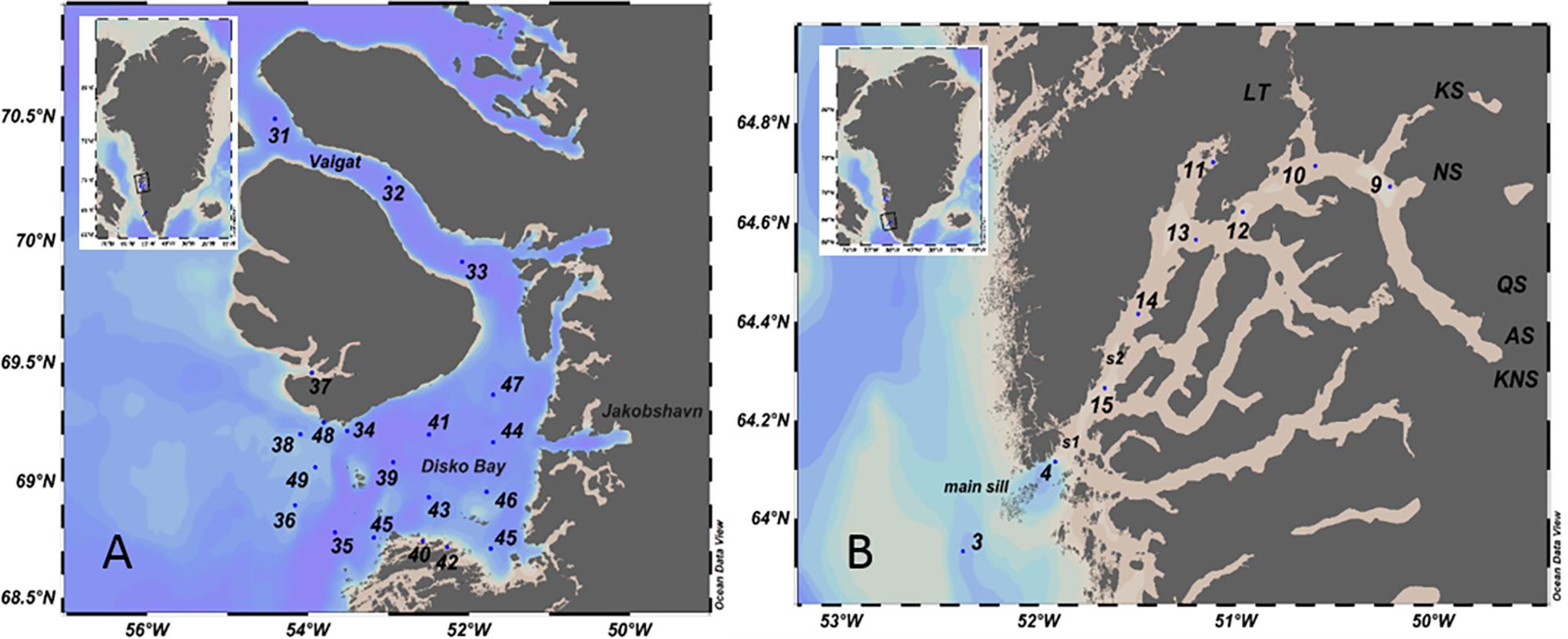
Figure 1. Area of study. Vaigat-Disko Bay (A) and Godthabsfjord (B), along southwest coast of Greenland. Summer campaign from June 26, 2017 to July 17, 2017 onboard research vessel Maria S. Merian (cruise ID MSM65). Numbers indicate sampled stations. Acronyms in panel (B) refer to marine terminating (KNS, Kangiata Nunata Sermia; AS, Akugdlerssup sermia; and NS, Narssap Sermia) and land terminating glaciers (QS, Qamanarssup Sermia; KS, Kangilinguata Sermia; and SS, Saqqap Semersua) in contact with the inner part of the fjord.

Godthabsfjord is a sub-arctic sill fjord, located on the southwest coast of Greenland (Figure 1B). Nuuk, the capital of Greenland is located at the mouth of the fjord. The fjord system is made up of a number of fjord branches and is therefore complex. Our study, however, is limited to the westernmost fjord branch, also considered the main fjord and the inner part of the main fjord. The inner part of the fjord is in contact with three land terminating: Qamanaarsup Sermia (QS), Kangilinnguata Sermia (KS), and Saqqap Sermersua (SS) which drains through lake Tasersuaq (LT); and three marine terminating glaciers of the GrIS: Kangiata Nunata Sermia (KNS), Akugdlerssup Sermia (AS), and Narssap Sermia (NS) that deliver glacial ice and meltwater to the fjord. The outer part of the fjord is characterized by several sills. The main sill at the entrance of the fjord is -170 m deep. Within 48 km of the main sill, there occurs a sequence of two additional sills (s1 and s2) with approximate depths of 250 and 277 m, respectively, (Mortensen et al., 2011). The fjord covers a distance of 187 km from the mouth to head with the width varying from 4.0 to 8.0 km. The fjord system covers an area of 2013 km² with an average depth of 250 m and a deeper (>600 m) basin.

Hydrography

We measured conductivity, temperature and depth (CTD) profiles using SBE 911plus CTD (Sea-Bird Scientific, United States) to understand the hydrography of the region. Details of the CTD system are available in Zielinski et al. (2018). Near-surface (1.0–4.0 m) water samples were simultaneously collected using a CTD rosette equipped with 24 × 20 L sampling bottles to estimate concentrations of each of the optically active constituents (OACs) [Chl-a, CDOM, total suspended matter (TSM), and ISM] and to derive the inherent optical properties (IOPs), mainly the spectral absorption coefficients. The sampling depth is located well within the first optical depth (FOD) for applicability in ocean color remote sensing algorithm development.

Water Sample Collection

Water samples were collected at discrete depths to determine the concentrations of OACs and derive IOPs. To estimate Chl-a concentration, 1.2–9.0 L of sample volumes were filtered through 0.7 μm glass fiber filters (GF/F Whatman, United States) under low vacuum and minimum light conditions to avoid bioactivity caused by ambient light. The filters were covered in aluminum foil and frozen onboard at -80°C until extraction in laboratory. Pigments were then extracted in 90% Acetone (Arar and Collins, 1997) and measured with a precalibrated TD 700 laboratory fluorometer (Turner Designs, United States).

Water samples, for CDOM estimation, were collected in amber colored glass bottles and filtered onboard, through 0.2 μm pore size membrane filters (Sartorius, Germany). The filtrate was immediately measured onboard, in dual beam UV-VIS-Spectrophotometer (UV 2700 Shimadzu, Japan) using 10 cm pathlength cuvettes with ultrapure water as reference. Samples were scanned at medium scan speed with an increment of 1 nm in the spectral range 200–800 nm. Sample cells were pre-rinsed twice with the sample to avoid contamination. Absorbance values A (λ) were baseline corrected and converted to absorption coefficients a_cdom (λ) following the equation:

$${\text{a}}_{\text{cdom}}\left(\lambda \right)\text{=}\frac{2.303*\text{A}\left(\lambda \right)}{l}\left(1\right)$$

where a_cdom (λ) is the spectral absorption coefficient of CDOM and I is the pathlength in meters. We consider the a_cdom at 350 nm as a quantitative measure of CDOM in this study.

To determine the TSM and ISM concentrations 0.9–15.0 L of water samples were filtered through precombusted and preweighed (Kern 770-60, KERN and SOHN, Germany) 0.7 μm pore size (GF/F, Whatman, United States) filters. The filters were frozen onboard at -20°C until analysis on land. Post-cruise the filters were allowed to thaw and dried at 60°C for at least 6 h. The filters were then cooled to room temperature and weighed for TSM concentration. The filters were then combusted at 500°C for 5 h and weighed again to provide the ISM concentrations (Bowers and Binding, 2006).

Water samples were also filtered and analyzed to determine total particulate, non-algal and phytoplankton spectral absorption coefficients (Yentsch, 1962; Kishino et al., 1985; Mitchell, 1990) using the quantitative filter technique (QFT). In this technique, particulate matter is concentrated onto filters via filtration and spectral absorbance measured directly in a spectrophotometer equipped with an integrating sphere. Depending on the turbidity in the water column 0.5–1.0 L of water samples were filtered onboard through 0.7 μm pore size filters (GF/F, Whatman, United States) under low vacuum. The filters were then covered in aluminum foil and frozen at -80°C until analysis in the laboratory. Post-cruise the optical density of the filters was measured using spectrophotometer with an integrating sphere (Cary 5000, Agilent Technologies, United States). Spectral absorption coefficients for the total particulate and non-algal fractions were then determined following Eq. (2) as per the IOCCG protocols (Roesler et al., 2018).

$${\text{a}}_{\text{x}}\left(\lambda \right)\text{=}\frac{{\left\{\ln {\left(\text{10}\right)}^{\text{*}}\text{0}.{\text{323}}^{\text{*}}{\left[{\text{OD}}_{\text{f}}\left(\lambda \right)\right]}^{\text{1}.\text{0867}}\right\}}^{*}}{\text{V}}\text{area }\left(2\right)$$

Where x refers to either the total particulate or the non-algal fraction of the total particulate absorption coefficient. OD_f (λ) refers to the blank corrected and averaged sample filter optical density, area refers to the effective area of the filter in m², 1.0867 refers to the amplification factor, and V refers to the volume of sample filtered in m³. Phytoplankton absorption coefficients were then obtained as the difference between total particulate and non-algal absorption coefficients.

In situ Bio-Optical Measurements

Water Transparency and Color

Water clarity and apparent color of the water were measured following traditional oceanographic methods using the Secchi disc (Wernand, 2010) and the Forel Ule comparator scale (Novoa et al., 2014), respectively.

Radiometric Profiles

Profiles of hyperspectral downwelling irradiance E_d (λ) and upwelling radiance L_u (λ) were measured using the free-falling profiler, HyperPro II (Sea-Bird Scientific, United States) equipped with ECO Puck Chl-a fluorescence and backscatter sensors. In addition to the Ed (λ) and L_u (λ) sensors, an above surface irradiance E_s (λ) sensor was also mounted at an elevated position on the vessel, free from any shadow. At each station, three consecutive casts were obtained in free falling mode. Pressure tare was applied on deck. In order to avoid ship shadow effects, the profiler was first allowed to drift at least 30 m away from the vessel. Measured raw signals were processed using the Prosoft software, version 7.7.16 (Sea-Bird Scientific, United States), provided by the manufacturer. Apparent optical properties of water, e.g., the diffuse attenuation coefficient of downwelling irradiance [K_d (λ)] and the remote sensing reflectance [R_rs (λ)] were obtained as level 3 and level 4 processing products, respectively. The data was binned every 1 m depth and 1 nm wavelength. Profiles measured with a tilt greater than 5° were not considered in the processing. Variance in the above surface irradiance was used to check for variations in incident solar light caused by passing clouds and casts with less than 10% variance in surface irradiance (E_s490) only were considered in the analysis. The solar zenith angle during the profiler operations varied between 41° and 78°.

Bio-Optical Sensor Package

Profiles of in situ spectral total non-water absorption [a (λ)] and beam attenuation [c (λ)] coefficients were obtained using a bio-optical sensor package. The package consisted of absorption-attenuation meter (ac-s, Sea-Bird Scientific, United States) backscattering sensor (ECO BB9, Sea-Bird Scientific, United States), CTD (Sea-Bird Scientific, United States) and a pump. The ac-s instrument, with a pathlength of 25 cm, measures a (λ) and c (λ) at 4 nm resolution in the 400–730 nm visible wavelength range while the ECO BB9 measures backscattering (b_b (λ)) at nine wavelengths (412, 440, 488, 510, 532, 595, 650, 676, and 715 nm). The package is installed in a custom-built frame and used to obtain in situ profiles of IOPs [a (λ), c (λ), b_b (λ)]. Before profiling, the package was lowered to a depth of 10 m for 10 min to provide effective purging, brought back to surface following which a profile was collected at low speed of approx. 0.5 ms^-1. Post-cruise, the profiles were processed in WAP processing software (version 4.37) provided by the manufacturer (Sea-Bird Scientific, United States). Post-processing, the casts were separated into downcasts and upcasts and depth binned at 0.5 m. The profiles were then corrected for temperature, salinity, blank, and scattering effects. The absorption coefficients were corrected for scattering errors according to Röttgers et al. (2013).

Radiative Transfer Modeling

For radiative transfer simulations, we used the commercially available radiative transfer model Hydrolight, version 5.3 (Sequoia Scientific, United States) extensively documented by Mobley (1994). Simulations were performed at five stations in the Vaigat-Disko Bay. The stations were chosen based upon availability of IOPs, AOPs and low cloud cover. The inbuilt “Measured IOP model” was chosen and IOP specifications, inelastic scattering processes and boundary conditions were provided as inputs. An overview of the various inputs is presented in Figure 2A. Downcasts of ac-s and BB9 with 0.5 m depth binning were used. Pure water absorption coefficients by Pope and Fry (1997) and scattering coefficients from Buiteveld et al. (1994) were considered. Fournier–Forand scattering phase function was chosen. All of the three sources of inelastic scattering, namely chlorophyll fluorescence, CDOM fluorescence and Raman scattering were accounted for with Chl-a concentration and CDOM absorption coefficients (a_cdom350) measured at subsurface and discrete depths. Mass-specific absorption coefficients of phytoplankton derived from measurements of phytoplankton absorption using the QFT, were also provided as input. Hydrolight default fluorescence efficiency was selected in all the runs. Measured surface irradiance was provided as total irradiance and Hydrolight inbuilt code RADTRAN was selected to calculate the direct and diffuse irradiance components. Station specific cloud conditions were specified and ocean bottom boundary condition was selected as optically deep.

FIGURE 2

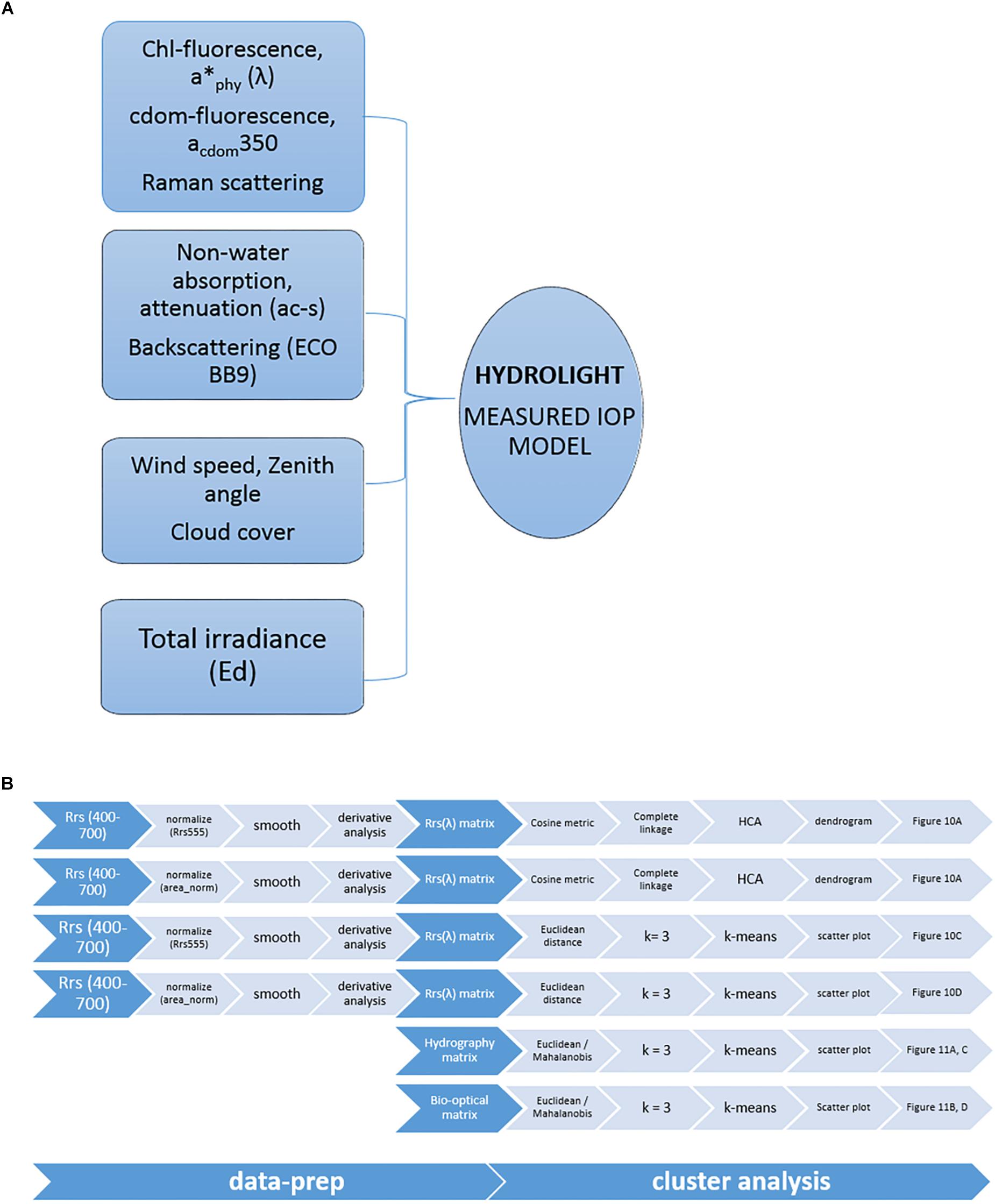
Figure 2. (A) Schematic of the radiative transfer model simulations in Hydrolight. For details, refer to section “Radiative Transfer Modeling.” (B) Schematic of cluster analysis of hydrographic and bio-optical data in the Vaigat-Disko Bay. For details, refer to section “Derivative and Cluster Analysis.”

Derivative and Cluster Analysis

The hierarchical cluster analysis (HCA) and the non-hierarchical k-means clustering methods were applied onto near-surface hydrographic and bio-optical data in the Vaigat-Disko Bay. Hydrographic matrix consisted of temperature and salinity data. Two bio-optical data matrices were formed, one with in situ hyperspectral Rrs (λ) and another with bio-optical parameters such as SDD, FUI, Euphotic depth (Z_eu), Chl-a, K_d490, K_par, K_d490_Z_eu, K_par_Z_eu. Description of the various parameters is listed in Table 1. In case of hyperspectral data, prior to cluster analysis, the spectra were normalized, filtered, and derivative analysis was performed. The fourth derivative spectra were then used in the cluster analysis. Figure 2B provides an overview of the steps involved in data preparation and cluster analysis of the different data matrices. HCA was performed using the cosine proximity metric and complete linkage method. The cosine is chosen as an appropriate metric in the analysis of Rrs spectra in this study as it reflects the differences in the spectral shape of the spectra and not the magnitude (Torrecilla et al., 2011). As the parameters of the bio-optical matrix strongly correlate, the Mahalanobis distance metric was also tested in addition to the Euclidean distance in k-means clustering.

Normalization

The cosine metric also has the advantage of being scale invariant and therefore insensitive to normalization of the Rrs spectra (Torrecilla et al., 2011). To check for this, we tested two different methods to normalize the hyperspectral Rrs. One method we refer to as “Rrs555” (Goncalves-Araujo et al., 2018) and the other as “area_norm” normalization method (Xi et al., 2015). In Rrs555, Rrs (λ) were normalized to Rrs at 555 nm. In area_norm, Rrs (λ) were normalized to the area, Ar, covered by the spectral curve over the wavelength range 350–750 nm, following Eqs 3 and 4.

$$\text{Rrs}\left(\lambda \right)\_\text{norm=}\frac{\text{Rrs}\left(\lambda \right)}{\text{Ar}}\left(3\right)$$

where Rrs (λ)_norm represents the area normalized Rrs curve and

$$\text{Ar=}\frac{{\int }_{{\lambda }_{\text{min}}}^{{\lambda }_{\text{max}}}\text{Rrs}\left(\lambda \right)d\lambda }{{\lambda }_{\max }-{\lambda }_{\text{min}}}\left(4\right)$$

λ_min and λ_max refer to the lower and upper integration limits of the spectra.

Smoothening

The next step involved derivative analysis, which increases noise in the spectral data. Therefore, the normalized Rrs spectra were first smoothened using the Savitzky-Golay filter. Based on literature (Torrecilla et al., 2011), a fourth order polynomial and a frame length of 21 was used in the filtering.

Derivative Analysis

For the derivative analysis, a finite divided difference algorithm was used to obtain the 4th derivative spectra over a sampling interval Δλ, defined as Δλ = λj–λi, where λj > λi. For reflectance spectra, 27 nm is reported to be appropriate (Torrecilla et al., 2011), and so we chose Δλ = 27 in our analysis. The first and the nth derivative were obtained following Eqs 5 and 6,

$$\frac{d\text{Rrs}}{d\lambda }\text{=}\frac{\text{Rrs}\left(\lambda \text{j}\right)-\text{Rrs}\left(\lambda \text{i}\right)}{\Delta \lambda }\left(5\right)$$

$$\frac{d^n\text{Rrs}}{d{\lambda }^n}\text{=}\frac{d}{d\lambda }\left[\frac{d^{n-1}\text{Rrs}}{d{\lambda }^{n-1}}\right]\left(6\right)$$

The fourth derivative spectra were then used as inputs in the cluster analysis. Normalization and derivative analysis of Rrs spectra enable detection of subtle features in the different types of Rrs spectra.

Results

Hydrography

The surface water salinities in the Vaigat-Disko Bay were influenced by surface ice-melt. Surface salinity in the bay, decreased from 33.44 outside the Bay to 31.83 near Jakobshavn Isbrae. Based on temperature and salinity distribution, we identified three distinct surface water masses in the Bay (Figures 3A,B): a glacial meltwater plume, Atlantic water mass and a frontal zone. The glacial meltwater plume was characterized by increased temperature and low salinity (7.5–8.0°C, 32.00–32.25) while the west Greenland current water mass exhibited low temperature and high salinity (1.0–3.0°C, 33.25–33.44). The frontal zone exhibited intermediate temperature and salinity ranges (3.5–7.0°C, 32.50–33.00). Shelf water masses that advect into the Bay were evident in the Temperature vs. Salinity (TS) plot (Figure 4C). The three surface water masses were also characterized by distinct densities (Figures 5C,I). The meltwater plume was characterized by a strong pycnocline (25.0–27.0 kg m^-3) while the frontal zone was characterized by a relatively weaker gradient (26.0–27.0 kg m^-3). The west Greenland current water mass featured no significant gradient.

FIGURE 3

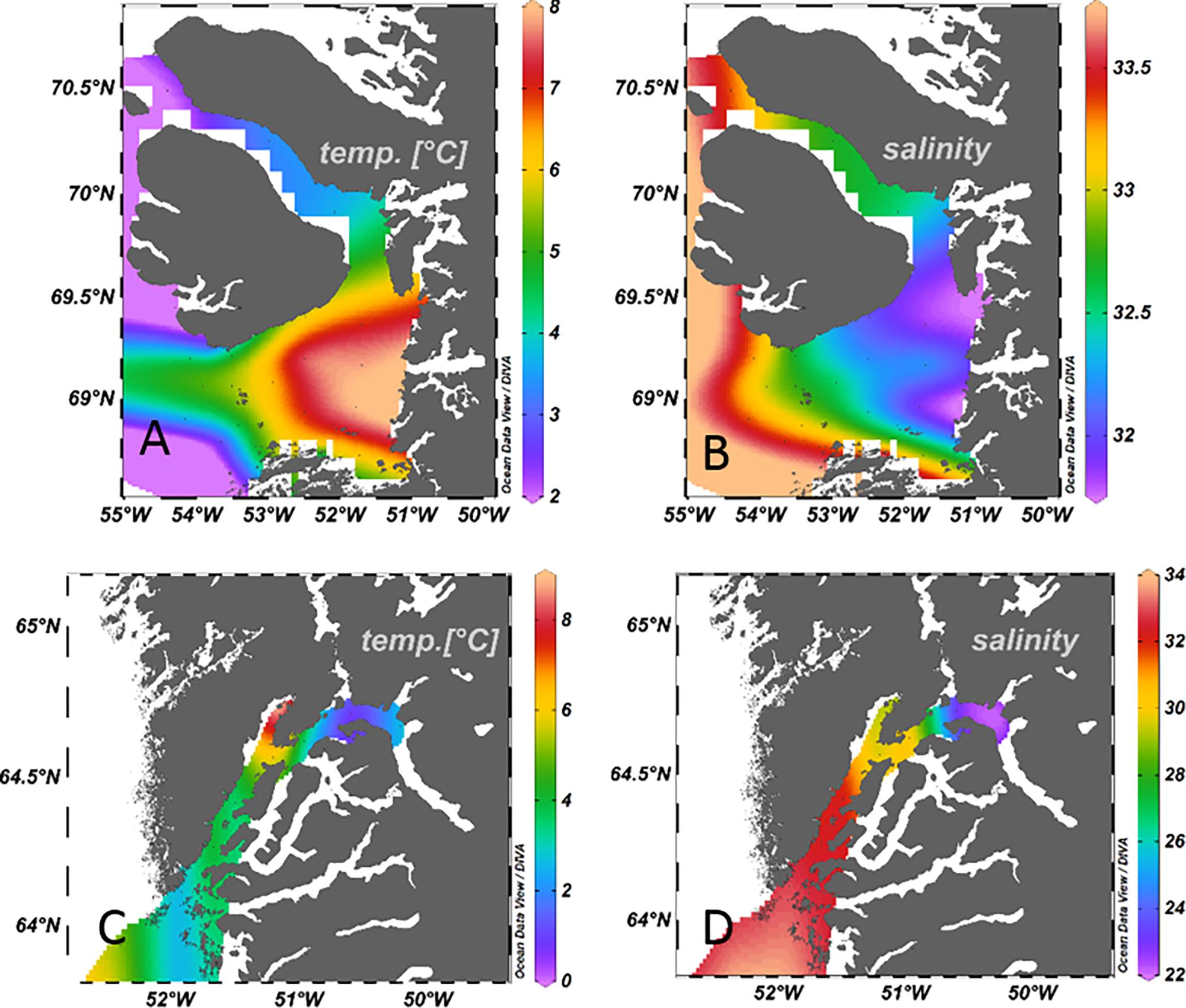
Figure 3. Hydrography in the Vaigat-Disko Bay and Godthabsfjord. Surface maps of temperature and salinity in the Vaigat-Disko Bay (A,B) and Godthabsfjord (C,D), respectively.

FIGURE 4

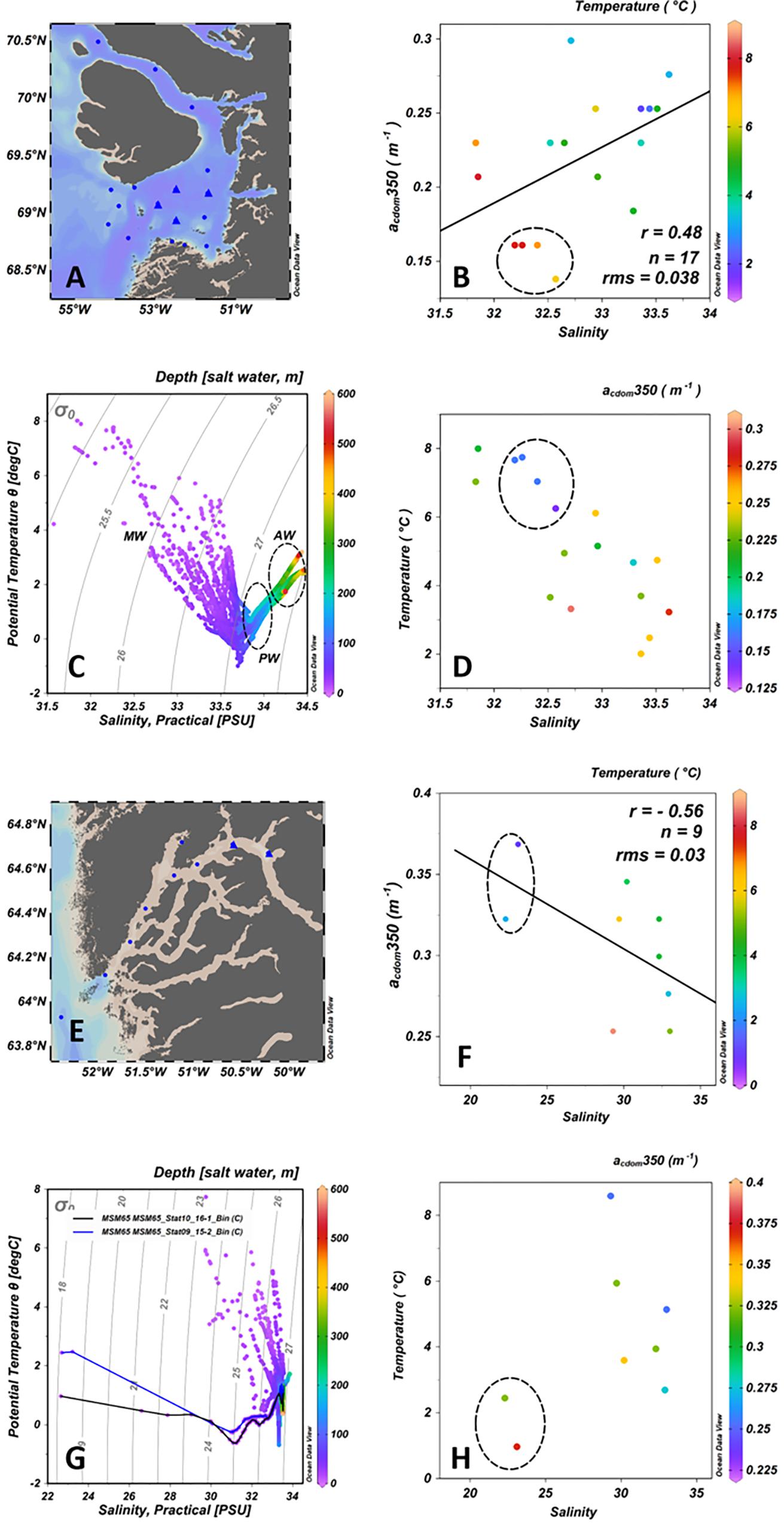
Figure 4. TS Plots and water masses in the (top panel) Vaigat-Disko Bay and (Bottom panel) Godthabsfjord. (A,E) Stations sampled in the Vaigat-Disko Bay and Godthabsfjord, meltwater core stations marked as triangles. (B,F) Regression of Salinity vs. a_cdom350 (r, correlation coefficient; n, number of data points; rms, root mean square). Color represents temperature as indicated in the colorbar. Data points enclosed in dashed circle represent meltwater core stations. (C,G) Scatter plot of salinity and potential temperature with isopycnals. Color represents depth as indicated in the colorbar. (D,H) Scatter plot of salinity and temperature. Color represents a_cdom350 as indicated in the colorbar. Data points enclosed in dashed circle represent meltwater core stations. Note that ranges in axes are different, representing the observed ranges in different parameters in the two areas of investigation.

FIGURE 5

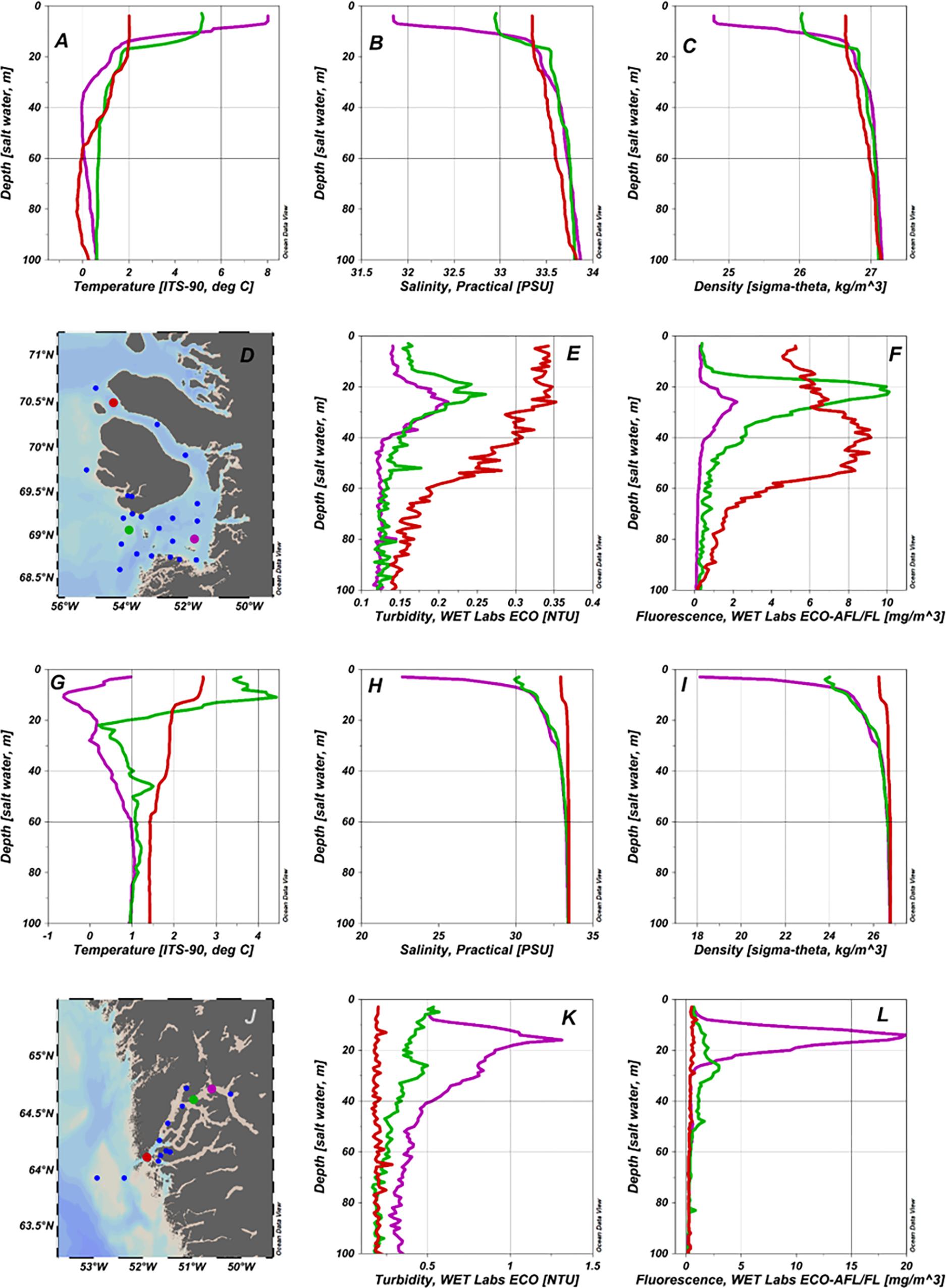
Figure 5. Depth profiles of hydrographic [temperature (A,G), salinity (B,H), density (C,I)] and bio-optical parameters [turbidity (E,K), Chla fluorescence (F,L)] at stations representing the three different water masses in the (top panel) Vaigat-Disko Bay and the (bottom panel) Godthabsfjord sections. (D,J) Stations sampled and representative stations marked. Note that ranges in axes are different, representing the observed ranges in the two areas of investigation.

In Godthabsfjord, sampling and profiling beyond station 9 (Figure 1B) was restricted due to sea-ice cover. Within the sampled stations, the salinity at the surface, ranged from 22.29 (station 9) to 33.05 (at station 3) outside the fjord (Figure 3D). Surface temperatures in the fjord ranged between 0.91 and 8.61°C (Figure 3C). Lowest temperatures were recorded in the inner section of the fjord while highest temperatures were recorded at station 11. For ease of interpretation, we shall consider stations 9 and 10, representative of inner fjord dynamics and bio-optics. Stations 12 and 13 lie within intermediate salinities (and so representative of mid fjord section) while stations 4, 14, and 15 as representative of outer fjord scenario. The wider range in salinity along with strong density gradient in inner Godthabsfjord is evident in the TS plot in Figures 4E,H. In contrast to meltwater stations in the Disko Bay, inner fjord stations in Godthabsfjord were characterized by low temperatures (Figures 4E–H).

Salinity vs. CDOM

Salinity vs. CDOM relationship were contrasting in the Vaigat-Disko Bay and Godthabsfjord. At stations sampled in the Vaigat-Disko Bay, salinity varied over a narrow range (31.83–33.44) and concentration of CDOM measured lowest in the meltwater core. Regression of a_cdom350 against salinity (Figures 4A,B) in the Vaigat-Disko Bay resulted in a positive relationship (n = 17, r = 0.48, rms = 0.038). In Godthabsfjord salinity varied over a wider range (22.0–33.0) and a_cdom350 measured high at stations sampled in the inner fjord (Figures 4E,F), resulting in a moderate inverse correlation (n = 09, r = -0.56, rms = 0.03).

Optically Active Constituents, Turbidity and IOPs

Near-surface Chl-a concentrations in the Vaigat-Disko Bay ranged between 0.12 and 2.27 mg m^-3. Highest pigment concentrations (1.95 and 2.27 mg m^-3) were measured at marine stations (31 and 35, respectively) in the bay. Intermediate concentrations (1.91, 0.92, and 0.96 mg m^-3) in the Bay, were observed at shallow stations (40, 42, and 48, respectively) close to the coast. Measured concentration range was the lowest (0.12–0.38 mg m^-3) in the meltwater plume. Concentrations of CDOM (a_cdom350 as proxy) in the Vaigat-Disko Bay ranged between 0.14 and 0.30 m^-1. Lowest coefficients (0.14–0.16 m^-1) were observed at core stations (39, 41, 43, and 44) in the meltwater plume. High coefficients (0.25–0.30 m^-1) were measured at marine stations sampled in the Vaigat (stations 31 and 32) and Disko Bay (station 35) and at shallow stations (40, 42, 45, and 48) close to the coast. Concentrations in the frontal zone were medium and ranged between 0.18 and 0.23 m^-1.

Total suspended matter concentrations in the Vaigat-Disko Bay ranged between 0.46 and 9.83 mg L^-1 while ISM concentrations ranged between 0.18 and 7.50 mg L^-1. Highest concentrations were observed at the marine station 31. Percentage of inorganic sediments in the TSM samples ranged from 28 to 76%. However, at most sampled stations, the percentage of organic matter was higher (23–71%) than inorganic contents, except at stations 31, 34, and 38 (58–76%). In the meltwater plume, the ISM concentrations ranged between 0.18 and 0.32 mg L^-1. Detailed ranges are presented in Table 2.

TABLE 2

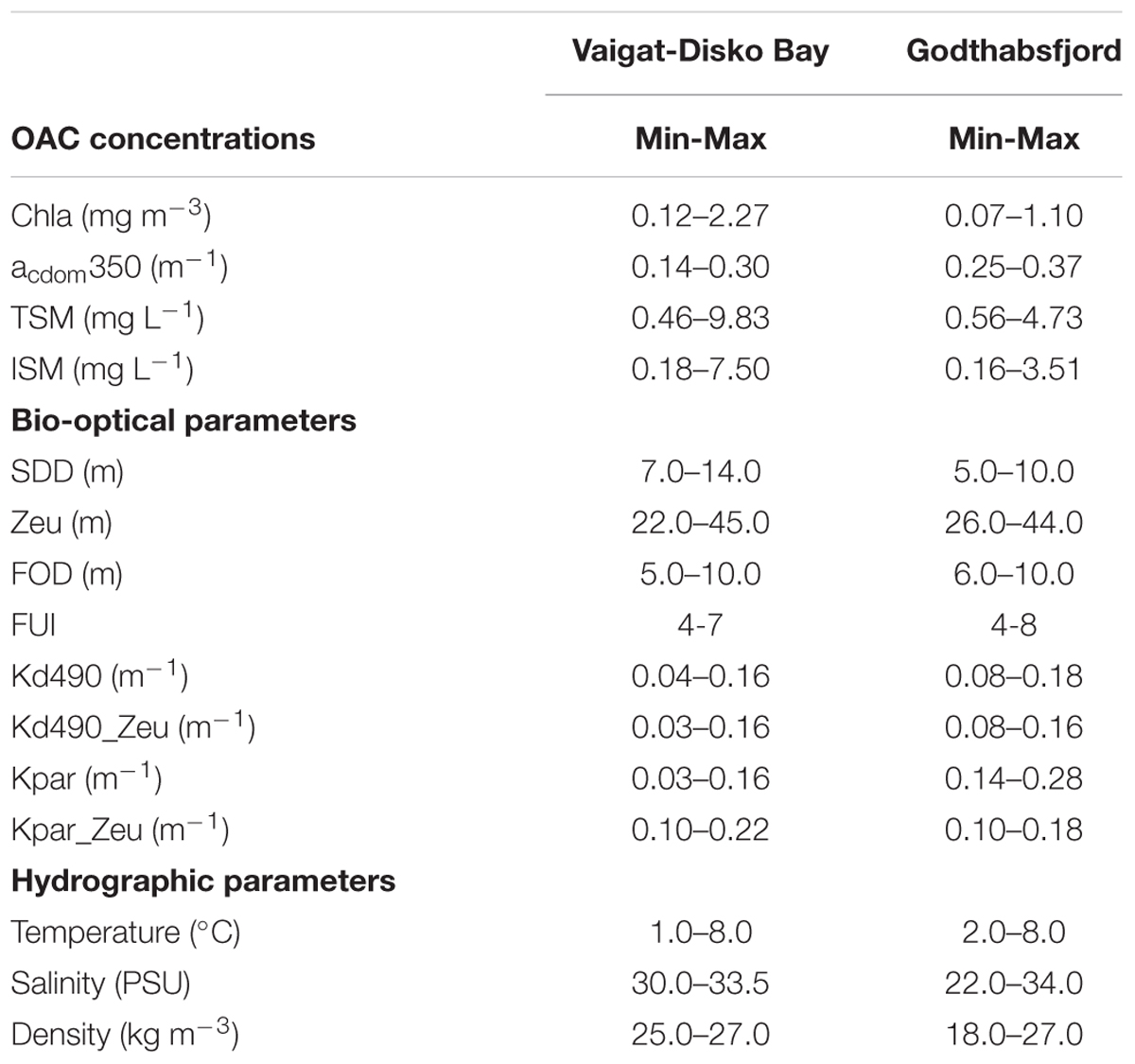
Table 2. Variability in near-surface OAC concentrations, bio-optical parameters, and hydrographic parameter ranges measured in the Vaigat-Disko Bay and Godthabsfjord along southwest coast of Greenland.

In Godthabsfjord, the near-surface Chl-a concentrations ranged between 0.06 and 1.10 mg m^-3. Lowest concentration was measured highest at station 11 and highest at station 12. Near-surface CDOM concentrations ranged from 0.25 to 0.37 m^-1. Highest concentrations were observed in the inner fjord while lowest concentrations were observed offshore. TSM and ISM concentrations at near-surface depths were high in the inner fjord (Table 2). Additionally, surface ISM concentrations were also very high (3.51 mg L^-1) at station 11. In the inner fjord, inorganic fraction of the TSM was higher than the organic.

Meltwater stations in the Vaigat-Disko Bay and inner Godthabsfjord stations exhibited contrasting turbidity profiles (Figures 5E,K). In the Vaigat-Disko Bay, low turbidity profiles characterized the meltwater stations while increased turbidity profiles characterized the outer marine stations. In contrast, inner Godthabsfjord stations were characterized by high turbidity and outer fjord stations by low turbidity. Similar contrasting features were also observed in chlorophyll fluorescence profiles measured at stations in the meltwater core in the Bay and in the inner fjord (Figures 5F,L).

Particulate absorption coefficients were higher in the inner Godthabsfjord than in the meltwater core (Figure 6). Phytoplankton absorption peaks were prominent in the particulate absorption spectra in the Vaigat, in frontal zone of the Disko Bay, and in the outer and mid Godthabsfjord, indicating low contribution from non-algal particles. At stations representing the meltwater core and the inner fjord, however, the primary absorption peak was less evident, indicating increased contribution from 4 the non-algal fraction.

FIGURE 6

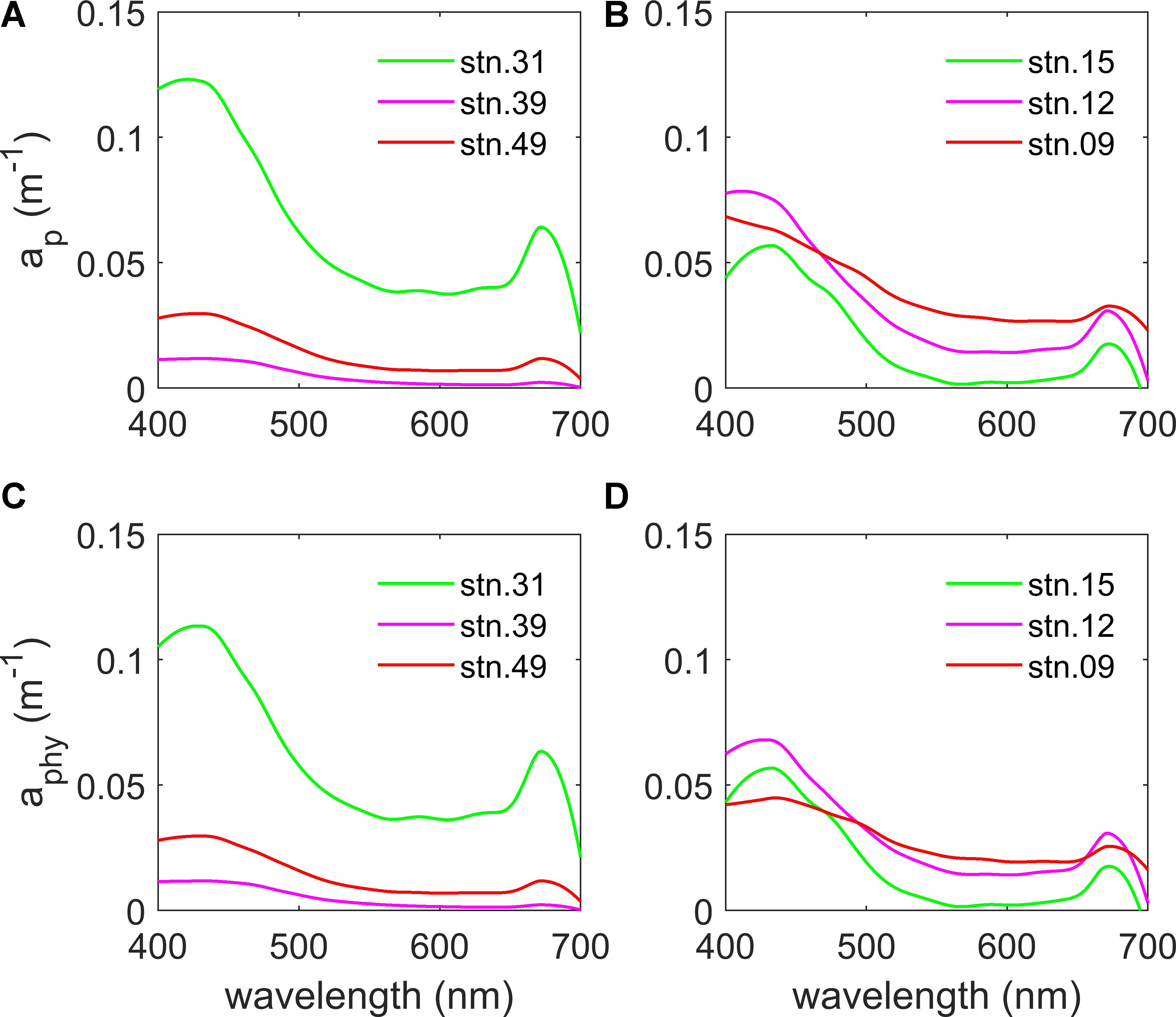
Figure 6. Spectral absorption properties of particulate (A,B) and phytoplankton pigments (C,D) at stations representing the three different water masses in Vaigat-Disko Bay (left panel) and sections in the Godthabsfjord (right panel).

Euphotic Depth and Diffuse Attenuation of PAR

Euphotic depth (Z_eu) determined from measured PAR profiles ranged between 22.0 and 45.0 m in the Vaigat-Disko Bay. Z_eu was shallow (22.0–24.0 m) at the productive stations with high Chl-a concentrations (40, 42) and at station 31 in the Vaigat, with highest concentration of ISM. Deepest values (40.0–45.0 m) of Z_eu were observed in the meltwater plume at stations 34, 41, 43, 44, 46, and 47. Diffuse attenuation coefficients of PAR averaged over the euphotic depths, K_par (Z_eu), were also determined from the measured PAR profiles. The K_par (Z_eu) coefficients ranged from 0.10 to 0.22 m^-1 in the Vaigat-Disko Bay. Minimum values of K_par (Z_eu) corresponded to stations with deep euphotic depths while maximum values of K_par (Z_eu) corresponded to shallow euphotic depths. Regression of K_par (Z_eu) against SDD in the Vaigat-Disko Bay, resulted in high coefficients of determinations (R² = 0.7, not shown here).

Euphotic depth in Godthabsfjord varied from 26.0 to 44.0 m. Deeper penetration of light (41.0–44.0 m) was observed at offshore station 3 and at the entrance (station 4) of the fjord. Inside the fjord, Z_eu reduced significantly (26.0–30.0 m). Inversely to Z_eu, high K_par (Z_eu) coefficients were observed at stations with shallow Z_eu and vice-versa. At stations offshore and at the fjord entrance a value of 0.10 m^-1 was measured while inside the fjord, the coefficient varied between 0.14 and 0.18 m^-1.

Forel Ule, Secchi Disc Depth, and First Optical Depth

In the Vaigat-Disko Bay, Forel Ule (FU) scale observations ranged between 4 and 7. FUI of 4 was observed at core stations (39, 41, 43, and 44) in the meltwater plume while 7 was observed at stations 32, 35, 40, and 42. Secchi depth (SDD) varied between 7.0 and 14.5 m. The SDD measured deeper (12.0–14.5 m) at stations in the meltwater plume and at stations sampled at the marine end. At stations 31, 35, 40, and 42 the measured SDD was relatively low (7.0–11.0 m). Low SDD values corresponded to stations with low Z_eu and high values to stations with high Z_eu. The FOD, derived as per Eq. 7 varied between 5.0 and 10.0 m.

$$\text{FOD=}\frac{Z_{eu}}{4.6}\left(7\right)$$

The FU index in Godthabsfjord ranged between 4 and 8 with the lowest index observed at the offshore station 3. The SDD was shallow compared to those measured in the Vaigat-Disko Bay and varied between 5.0 and 10.0 m. The lowest SDD was observed at station 11.

Diffuse Attenuation of Downwelling Irradiance

In the Vaigat-Disko Bay, the surface diffuse attenuation coefficients of downwelling irradiance (K_d490) ranged between 0.042 and 0.164 m^-1 (Figure 7A). High values (0.123–0.164 m^-1) were observed at shallow stations (40, 42) close to the coast and at the entrance stations in the Vaigat (31) and the Disko Bay (35, 36). At stations (41, 43, and 45) in the meltwater core the values observed were lowest and ranged between 0.052 and 0.053 m^-1. Around the meltwater core (45, 46, 47) and the frontal zone (32, 33, and 49), the coefficient varied from 0.061 to 0.090 m^-1.

FIGURE 7

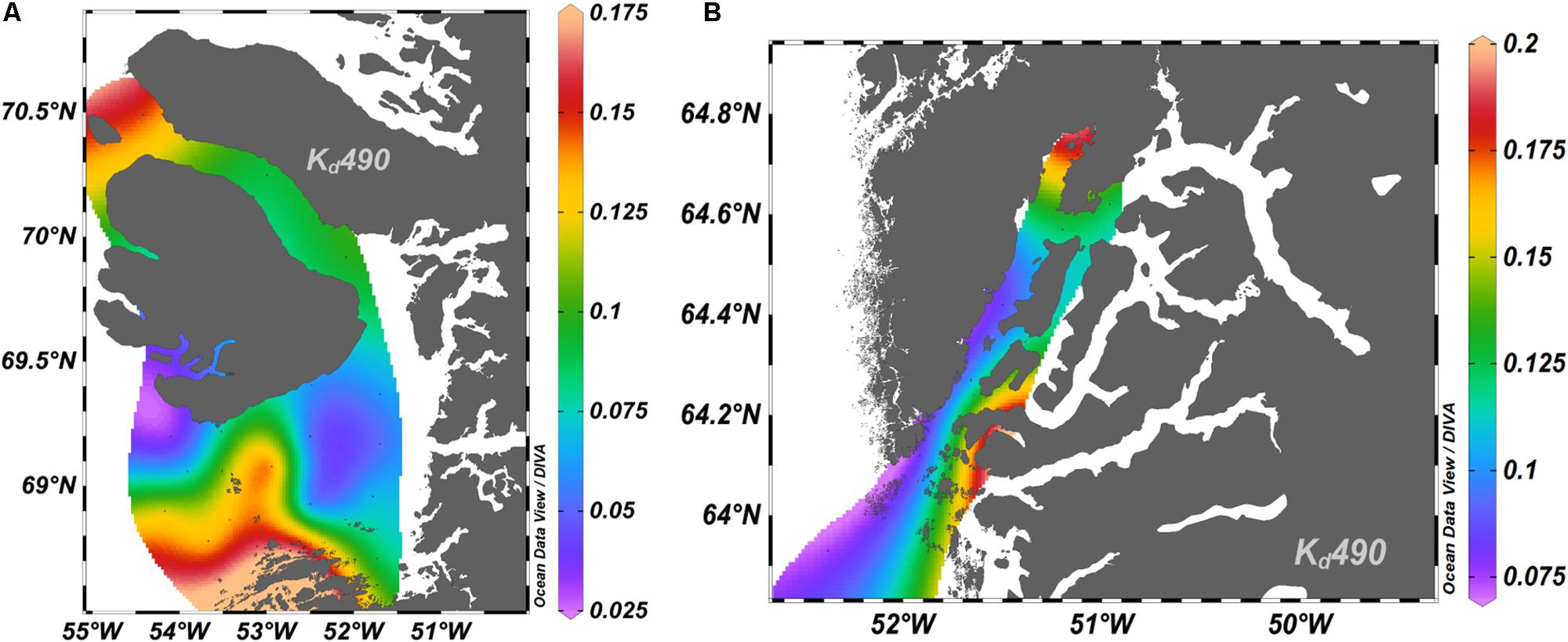
Figure 7. Diffuse attenuation coefficient (K_d490). Surface distribution maps of K_d490 in the Vaigat-Disko Bay (A) and in Godthabsfjord (B).

In Godthabsfjord, radiometric profiler operations were restricted due to sea ice cover and so casts were not obtained in the inner fjord. In the mid and outer fjord the coefficients ranged from 0.075 to 0.181 m^-1 (Figure 7B). Highest values were observed at station 11 while lowest were observed at stations offshore (station 3) and at the entrance (station 4) of the fjord.

1% Spectral E_d

Depths of spectral 1% downwelling irradiance E_d (λ) were derived from measured profiles of downwelling irradiance (Figure 8). In the Vaigat-Disko Bay spectral light traveled deepest in the meltwater plume, to a depth of about 52.0 m. In the frontal zone, the maximum depth of penetration was -35.0 m while at stations with medium to low pigment concentration was -32.0 m. Three different spectral types were observed. The spectra at stations in the meltwater plume and at stations with medium to low pigment concentrations were V-shaped while those in the frontal zone were U-shaped. In the meltwater plume region with high ISM concentrations, characterized by V-shaped spectra, green wavelength (500 nm) penetrated deepest into the water column while those at stations with medium to low pigment concentration, 560 nm penetrated deepest. In the frontal zone, with U shaped characteristic spectra, 500-560 nm wavelength range traveled the deepest.

FIGURE 8

Figure 8. Spectral types of 1% downwelling irradiance (E_d) in the Vaigat-Disko Bay (A) and Godthabsfjord (B). U shaped (blue) spectral type with 500–560 nm, V shaped (red) spectral type with 560 nm and V shaped (black) spectral type with 500 nm penetrating deepest in the water column.

The three spectral types observed in the Vaigat-Disko Bay were also evident in Godthabsfjord (Figure 8B). At the entrance station 4, the spectrum was V-shaped, with the blue – green wavelength (490 nm) penetrating deepest, to a depth of 61.0 m. At station 15, in the outer fjord, the spectrum was V shaped, with the green, 560 nm wavelength reaching a depth of 36.0 m. In the mid-fjord, at station 12, the spectrum was U shaped, with green wavelength band 500–560 nm traveling to a depth of 31.0 m.

Rrs Spectra or AOP Matrix

We observed variability in Rrs spectra in the Vaigat-Disko Bay (Figure 9A). Rrs spectra at the offshore stations and the glacial meltwater plume region of the bay peaked between 400 and 500 nm wavelength range. These spectra resemble case-1 water type reflectance spectra, despite the high ISM concentrations (Table 2). At shallow stations (40, 42) with high Chl-a concentrations (and therefore a strong fluorescence peak in the longer wavelength) along the coast in the Disko Bay, the spectra peaked between 500 and 550 nm while others at stations (31 and 45) with intermediate Chl-a concentrations peaked at 500 nm with relatively weaker fluorescence peak. Rrs (λ) variability was evident in Godthabsfjord as well (Figure 9B). The spectrum at offshore station 3 resembled case-1 water type spectra with a broad peak in the 400–500 nm wavelength range. Spectra at stations in the outer fjord peaked at 490–500 nm. In the mid fjord, spectra exhibited broad peaks in 500–550 nm range, with steep increase between 400 and 500 nm.

FIGURE 9

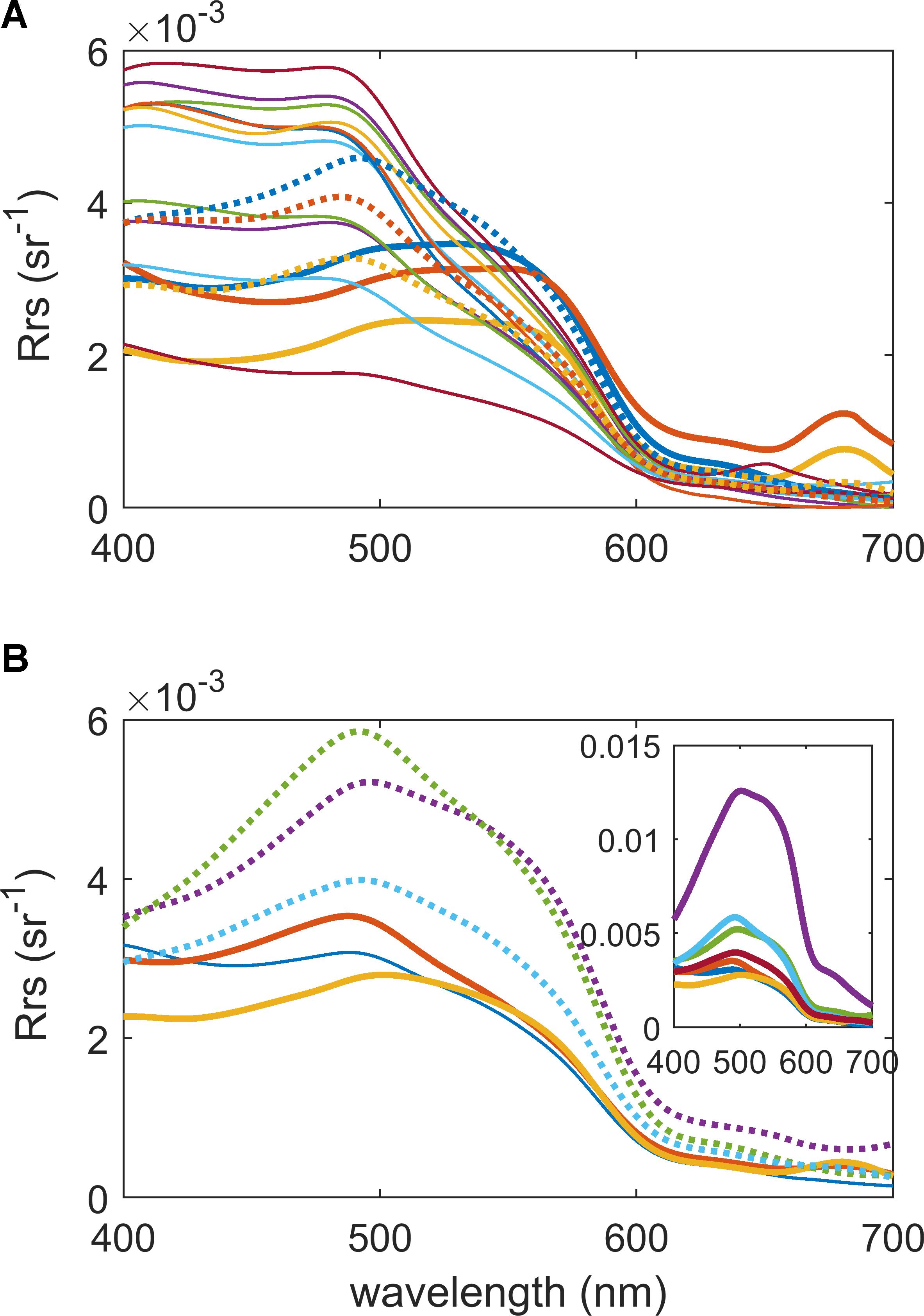
Figure 9. Hyperspectral variability in remote sensing reflectance (Rrs) in the Vaigat-Disko Bay (A) and Godthabsfjord (B). (A) Rrs spectra measured at stations in the glacial meltwater plume (thin solid lines), at stations with high Chla concentrations (thick solid lines) and with low Chla concentrations (dotted lines). (B) Rrs spectra measured at marine station 3 (thin solid line), in outer fjord (thick solid lines) and in mid fjord (dotted lines). Inset: Rrs spectral variability including spectra of highest magnitude in Godthabsfjord.

Hierarchical and Non-hierarchical Clustering of the Rrs Matrix

In order to test whether clustering algorithms were capable of resolving the above-described Rrs (λ) spectral variability in the Vaigat-Disko Bay, we applied the HCA and the non-hierarchical, k-means clustering methods onto in situ measured Rrs (λ). Resulting clusters are presented in the form of dendrogram (HCA) and scatter plots (k-means) in Figure 10. Figure 10A represents the dendrogram obtained from HCA (cosine, complete linkage) of Rrs (λ) normalized following the two normalization methods, Rrs555 and area_norm (see section “Normalization”). HCA was performed using the cosine proximity metric and complete linkage method. The cosine proximity metric being scale invariant, results in similar clusters irrespective of the normalization method. Figures 10C,D represent scatter plots of stations clustered using the k-means clustering (two normalization methods). The clusters obtained in k-means match those obtained in HCA, except for station 32 following the Rrs 555 normalization method. Cluster represented in green includes stations with case-1 type Rrs spectra, with peaks in the blue range of the visible spectrum (Figure 9, see section “Rrs Spectra or AOP Matrix”). Cluster represented in blue includes stations with case-2 type spectra corresponding to stations 40 and 42, with peaks in the green range of the visible spectrum. Lastly, cluster 3 comprise of stations with Rrs spectra peaking at 500 nm, corresponding to stations 31, 35, and 45.

FIGURE 10

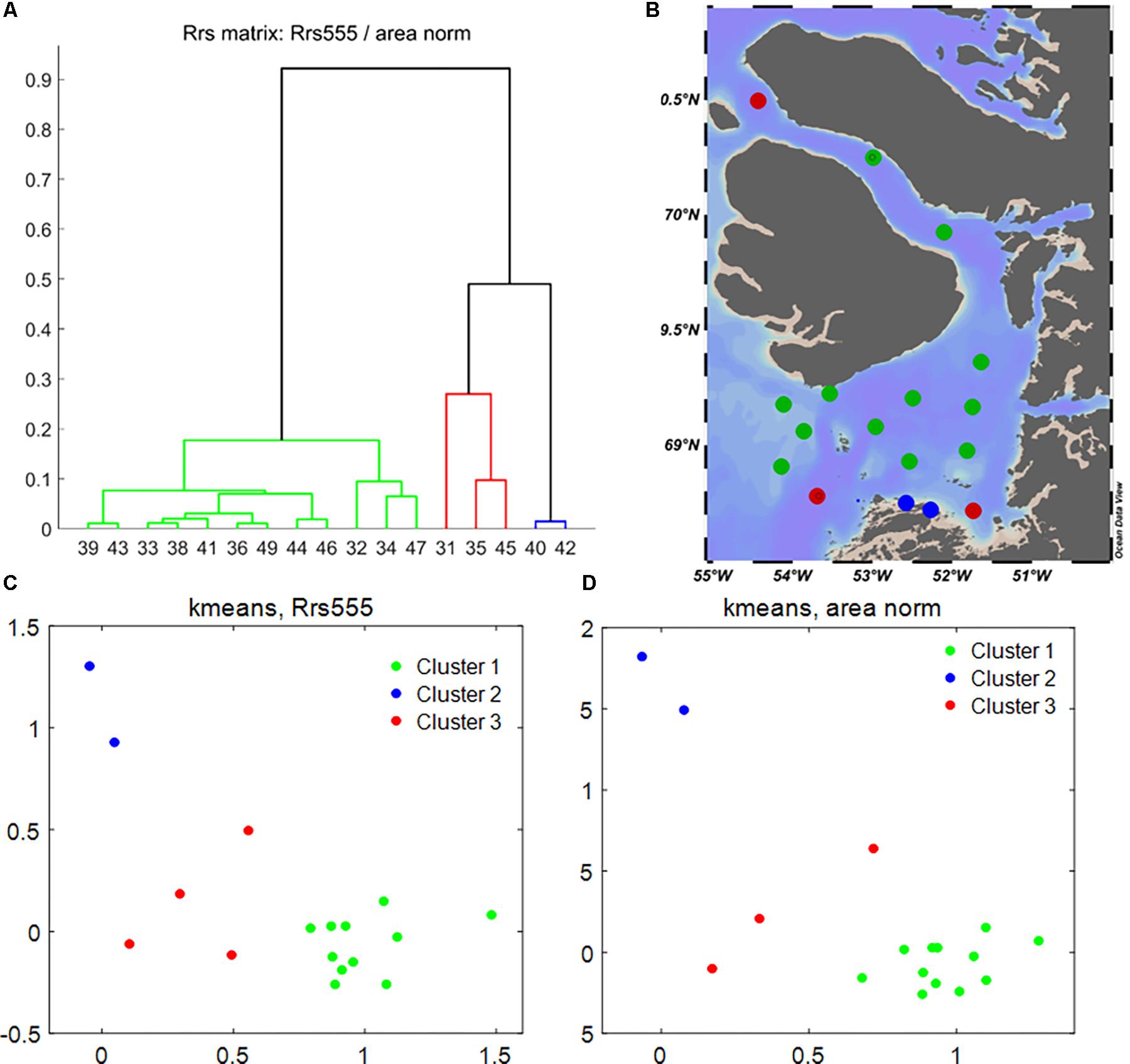
Figure 10. Cluster analysis of Rrs spectra. Dendrogram (A) of hierarchical cluster analysis (cosine proximity metric) of Rrs spectra normalized following the Rrs555 and the area_norm method. (B) Geographic distribution of clusters in the Vaigat Disko Bay. Scatter plot representing clusters derived using k-means clustering (Euclidean distance) following the Rrs555 (C) and the area_norm method (D).

Non-hierarchical Clustering of Hydrographic and Bio-Optical Matrices

We applied the k-means clustering method onto hydrographic and bio-optical matrices individually, to test if the bio-optical properties clustered in optical domains defined by hydrography of the region around the Vaigat-Disko Bay. The k-means clustering algorithm has been widely used in clustering of spectral as well as discrete optical datasets (Palacios et al., 2012; Spyrakos et al., 2018). In contrast to HCA, the algorithm requires the number of clusters to predetermined and provided as input (i.e., the value of k). Based on the surface features of temperature, salinity and Kd490 observed in Figures 3, 7 (see sections “Hydrography” and “Forel Ule, Secchi Disc Depth and First Optical Depth”), we set the value of k as 3. Clustering was tested using two different proximity metrics, the Euclidean and the Mahalanobis distance. The Mahalanobis distance considers the covariance of the data and the scales of the different variables.

The hydrographic matrix consisted of sub-surface (3.0–4.0 m) temperature and salinity data. Using the Euclidean distance metric, the following clusters were obtained, depicted in blue, green, and magenta, respectively, in Figure 11A.

FIGURE 11

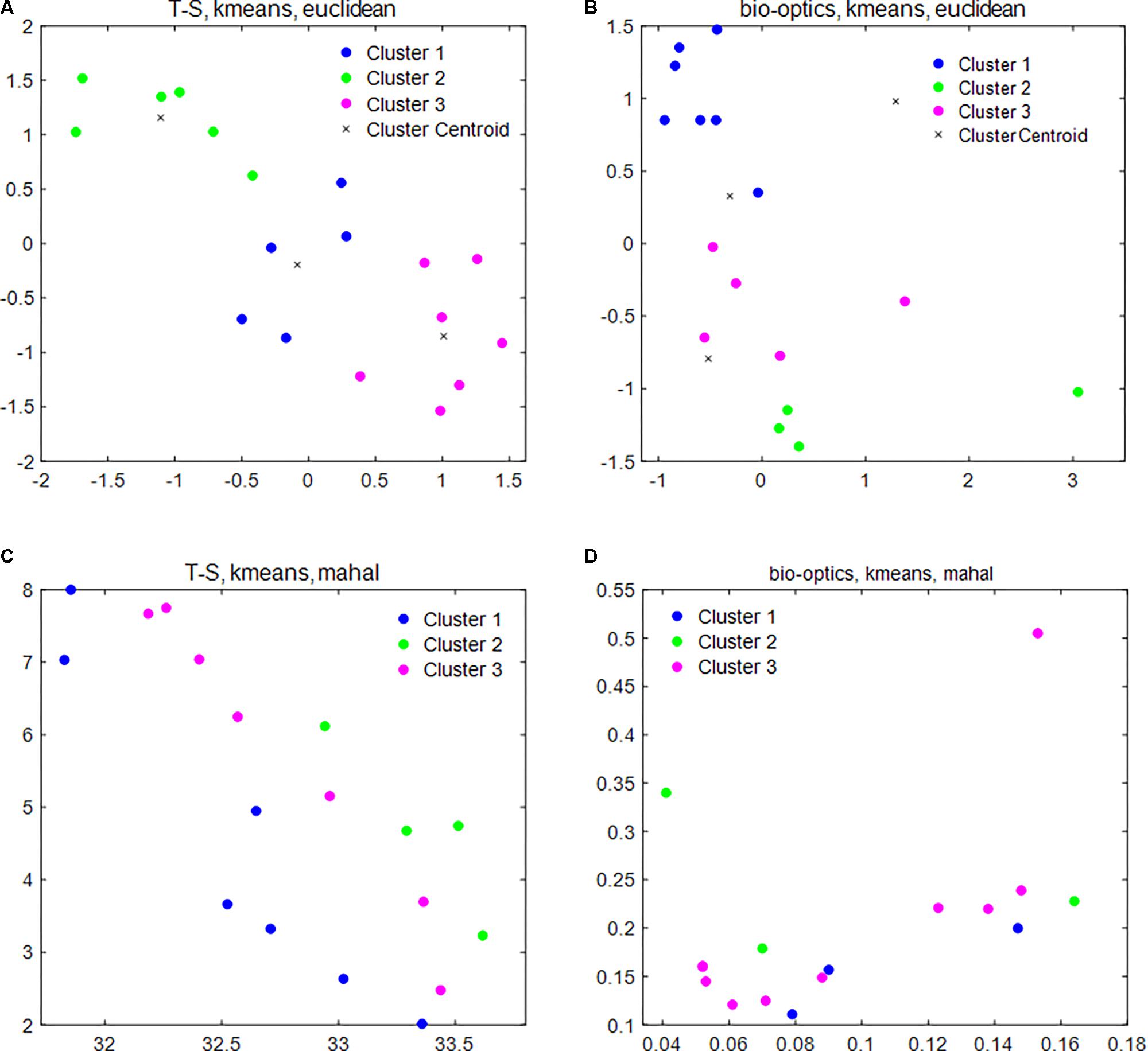
Figure 11. Cluster analysis of hydrographic and bio-optical matrices. Scatter plot representing clusters derived using k-means clustering of the hydrographic (A,C) and bio-optical matrices (B,D) using the Euclidean (A,B) and Mahalanobis distance metrics (C,D).

Cluster 1: 32, 33, 34, 45, 49

Cluster 2: 39, 41, 43, 44, 46, 47

Cluster 3: 31, 35, 36, 38, 40, 42, 48

Cluster 1 consisted of stations in the Atlantic water mass while cluster 2 consisted of stations in the meltwater plume. Cluster 3 consisted of stations forming the frontal zones with intermediate T-S characteristics between the Atlantic and the meltwater plume.

The bio-optical matrix consisted of SDD, FUI, Z_eu, Chl-a, K_d490_Z_eu, K_par_Z_eu. Description of the various terms is presented in Table 1. Using the Euclidean distance, following three clusters were obtained, depicted in blue, green, and magenta, respectively, in Figure 11B.

Cluster 1: 34, 39, 41, 43, 44, 46, 47

Cluster 2: 31, 35, 40, 42

Cluster 3: 32, 36, 38, 45, 49

Considering the Mahalanobis distance in k-means clustering of the hydrographic matrix, resulted in the following clusters depicted in blue, green, and magenta, respectively, in Figure 11C

Cluster 1: 31, 32, 33, 34, 46, 47, 48

Cluster 2: 38, 40, 42, 45

Cluster 3: 35, 36, 39, 41, 43, 44, 49

while clustering of the bio-optical matrix resulted in clusters as follows, depicted in blue, green, and magenta, respectively, in Figure 11D.

Cluster 1: 32, 34, 39

Cluster 2: 38, 40, 49

Cluster 3: 31, 35, 36, 41, 43, 44, 45, 46, 47

Comparing the resulting clusters obtained from the two distance metrics, Euclidean distance appears to perform better than the Mahalanobis distance for this combination of hydrographic and bio-optical matrices. Using the Euclidean distance 13 of the 16 stations group in similar clusters. However, using the Mahalanobis distance, the number is reduced to eight.

Optical Closure

Apparent optical properties were modeled using the Hydrolight radiative transfer model version 5.3 at five stations in the Vaigat-Disko Bay. Measured IOPs (a (λ), c (λ), b_b (λ)) were provided as inputs to the model (Figure 2). Modeled AOPs, specifically Rrs (λ) were then compared with in situ measured AOPs. Calculation (Eq. 8) of root mean square error (RMSE) provided information on the agreement between modeled and measured Rrs (λ).

$$\text{RMS}\text{Error}=\sqrt{\frac{{\sum }_{i=1}^n{\left({\text{Rrs}}_{\text{meas}}-{\text{Rrs}}_{\text{mod}}\right)}^2}{n}}\left(8\right)$$

Rrs__mod and Rrs__meas refer to modeled and measured Rrs, respectively, and n to the number of data points at each of the tested wavelengths. Figure 12 represents results of the closure test performed. Closure was most effective at longer wavelengths (615–675 nm; low RMSE; 0.00031 and 0.00038, respectively) while the highest errors were obtained at 485, 515, and 555 nm (0.00098, 0.00113, and 0.00118, respectively). According to stations, the calculated errors were highest at stations in the meltwater plume. The high values of RMSE could be attributed to the increased concentrations of ISM in the meltwater plume released along with the meltwater which are known to be highly scattering.

FIGURE 12

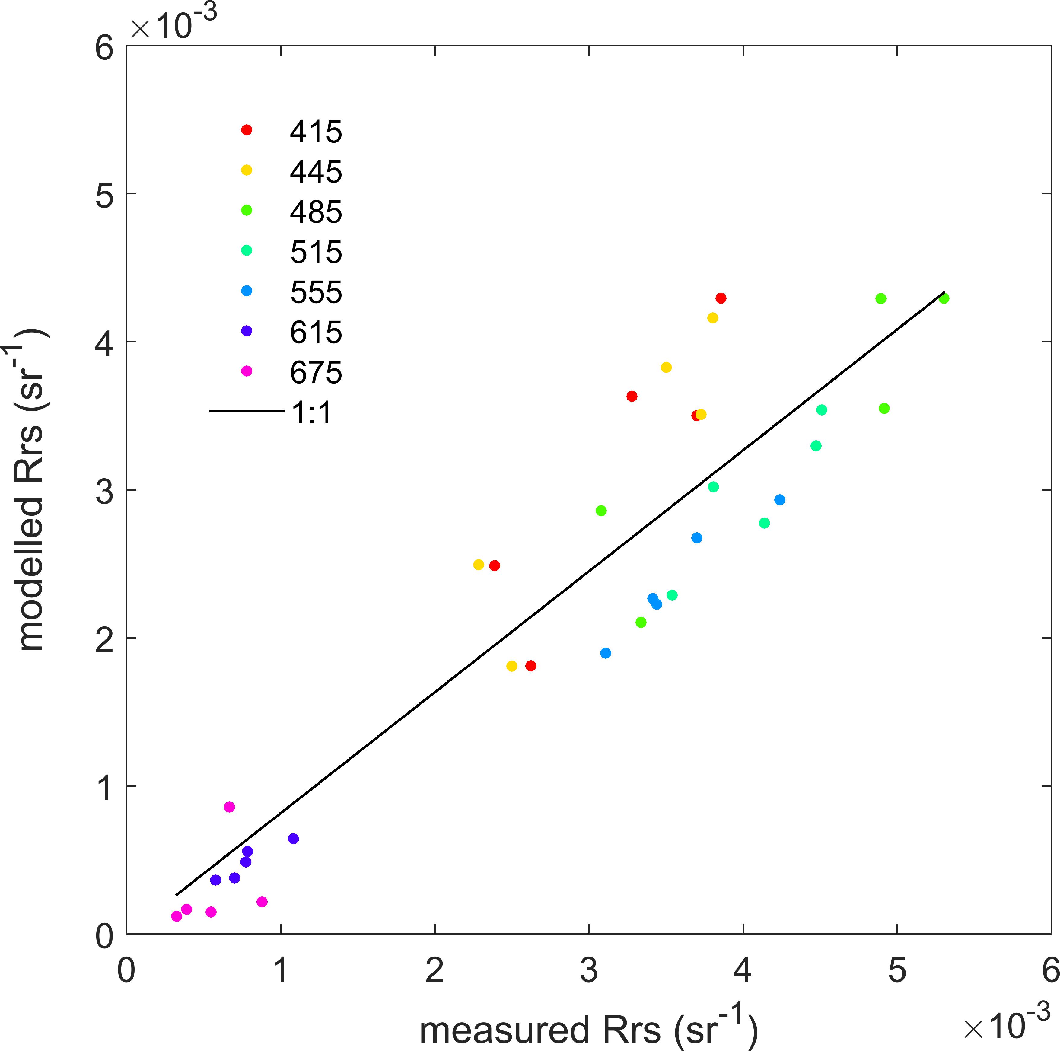
Figure 12. Optical closure of Rrs. Line of 1:1 agreement between the measured and modeled remote sensing reflectance (Rrs) at wavelengths 415, 445, 485, 515, 555, 615, and 675 nm.

Discussion

Hydrography Driven Bio-Optical Domains

The increasing extent of the meltwater plume in the Vaigat-Disko Bay and Godthabsfjord is evident in the surface distribution maps of temperature and salinity (Figures 3A,B). The meltwater plume in the Vaigat-Disko Bay was characterized by low salinity and increased temperature. The increased temperature is attributed to atmospheric sea-surface heating (Heide-Jørgensen et al., 2007). Density profiles (Figure 5) obtained in the regions provide further evidence of the effect of meltwater. Near-surface features of temperature and salinity when compared to those of diffuse attenuation coefficient (Figure 7) indicate three different bio-optical domains. It can be easily deduced from the figures that optical domains are indeed driven by the hydrodynamics of the region. Glacial meltwater and riverine runoff-influenced variability in IOPs and particulate matter distribution has also been investigated in fjords along Spitsbergen (Sagan and Darecki, 2018). Characterized by low CDOM concentrations, glacial meltwater is also evident in surface scatter plots of temperature vs. salinity (TS plots) with a_cdom350 as z variable (Figures 4D,H). Bio-optical variability influenced by physical oceanography processes has also been reported in the Tasman Sea (Cherukuru et al., 2016). Furthermore, application of machine learning techniques such as cluster analysis (Figures 11A,B) proved efficient in clustering the bio-optical domains in correspondence with hydrographic regions or water masses in the Vaigat-Disko Bay (Figures 11A,B). In another study with the application of HCA onto datasets consisting of hydrographic parameters and IOPs Goncalves-Araujo et al. (2018) proposed classification of the central-eastern Arctic Ocean into five different bio-optical provinces.

Salinity vs. CDOM

The inverse relationship between salinity and CDOM absorption coefficients in freshwater influenced coastal systems, such as the shelf seas, fjords, and estuaries is a well-known feature (Bowers et al., 2004; Bowers and Brett, 2008; Pavlov et al., 2016). Along the North-West coast of Norway, with observed salinity range of 20.0–33.0, and a_cdom443 ranging from 0.55 to 0.94 m^-1, Mascarenhas et al. (2017) reported R² as high as 0.91 in Trondheimsfjord. In contrast, in the Disko Bay (Figure 4B), the correlation between salinity and CDOM concentration (0.14–0.30 m^-1) was moderately strong but positive (R² = 0.51). The positive correlation can be attributed to the low CDOM concentrations in the meltwater plume compared to stations at the marine end. Positive correlation between salinity and cdom proxies have also been reported in embayments influenced by glacial meltwater along East Greenland shelf (Stedmon et al., 2015) and on the east coast of Novaya Zemlya (Glukhovets and Goldin, 2019). Furthermore, in contrast to typical fjord geography, bays have wider spatial coverage and therefore increased mixing and dilution, which restricts the salinity to a narrow range (31.83–33.44).

In Godthabsfjord (Figure 4F) despite salinity variations over a comparatively wider range (Table 2) and high CDOM concentrations in the inner fjord the inverse relationship was weak (r = -0.56). The weakening of the relationship, in meltwater-influenced fjord, could be attributed to low degree of variability in CDOM concentration (0.25–0.37 m^-1) between the freshwater influenced inner fjord and marine water influenced outer fjord stations (Table 2). However, the observed correlation coefficient in Godthabsfjord is higher than the coefficient (R² = 0.19) reported by Lund-Hansen et al. (2010) in Kangerlussuaq fjord, also located along the South-West coast of Greenland (salinity: 5.0–29.0, a_cdom440: 0.046–0.36 m^-1). In fjord ecosystems, the conservative relationship is strongly influenced by the type of freshwater sources that drain into a fjord. The conservative relationship is strong in fjords influenced by high riverine flux, rich in CDOM content, e.g., the Trondheimsfjord, along the North-West coast of Norway (Mascarenhas et al., 2017). However, in fjords influenced by increased glacial meltwater (Vaigat-Disko Bay) or a combination of both (Godthabsfjord) the relationship is observed to either reverse or weaken (Stedmon et al., 2015; Glukhovets and Goldin, 2019).

Hyperspectral Underwater Light Availability

The euphotic depth, defined as the depth of 1% of the measured near-surface PAR, was recorded deepest in the meltwater plume in the Vaigat-Disko Bay and at the entrance station, station 4, in the outer Godthabsfjord. In the spectral depth analysis of one percent downwelling irradiance, three spectral types were identified along fjord transects. The three spectral types identified (Figure 8A) correspond to the abundance of OACs in the fjord sections along transects. In the meltwater plume of the bay, the V-shaped spectra with 500 nm wavelength traveling deepest, correspond to stations with low OAC concentrations while the V-shaped spectra with 560 nm wavelength traveling deepest correspond to stations with medium to high concentrations of OACs. The U-shaped one percent irradiance spectra with 500–560 nm traveling deepest correspond to low to medium OAC concentrations. In Godthabsfjord as well (Figure 8B), the V-shaped spectra with 500–560 nm wavelengths traveling deepest in the water column corresponded to stations with low and high OAC concentrations, respectively, while the U shaped spectra at stations with intermediate OAC concentrations. Similar U and V-shaped spectral types along fjord transects have been earlier reported in Sognefjord and Trondheimsfjord along the Norwegian coast (Mascarenhas et al., 2017). The meltwater stations in the Bay are characterized by low OAC concentrations. The V-shaped one percent spectra with -500 nm penetrating deepest in the water column of the meltwater plume, correspond to stations with Rrs spectra that peak in the 400–500 nm wavelength range (Figure 9A) whereas the sections with high OAC concentrations and V-shaped one percent spectra with -560 nm traveling deepest in the water column correspond to stations with Rrs spectra that peak in the 500–550 nm wavelength range (Figure 9A).

Derivative and Cluster Analysis

Hierarchical cluster analysis (Figure 10A) and k-means (Figures 10C,D) clustering methods proved effective at resolving the spectral variability in Rrs presented in section “Rrs Spectra or AOP Matrix” (Figure 9). The analysis distinctly clustered stations with case-1 and case-2 type reflectance spectra (see section “Hierarchical and Non-hierarchical Clustering of the Rrs Matrix”). Being scale invariant, the cosine proximity metric in HCA, resulted in similar clusters (Figure 10A) irrespective of the normalization methods. The k-means algorithm also effectively clustered stations into similar clusters (Figures 10C,D).

In optical oceanography, hyperspectral data has been commonly analyzed using derivative spectroscopy. It has been applied to both inherent and apparent optical properties (Torrecilla et al., 2011; Xi et al., 2015; Goncalves-Araujo et al., 2018; Wollschläger et al., 2018). The derivative analysis does not only enhance spectral features but also, in case of AOPs, the derivative spectra are less affected by possible fluctuations in the incident light conditions. However, in order to derive effective spectral details, Torrecilla et al. (2011) recommend the sampling interval or band separation, Δλ, be carefully decided. Using the Rrs555 in HCA, Torrecilla et al. (2011) demonstrated discrimination of phytoplankton pigment assemblages in the open ocean under non-bloom conditions. Xi et al. (2015) reported the efficiency of HCA in clustering phytoplankton taxonomic groups derived from Hydrolight simulated Rrs (λ). Uitz et al. (2015) assessed the ability of hyperspectral optical measurements to discriminate changes in the composition of phytoplankton communities in open-ocean non-bloom conditions. Neukermans et al. (2016) used HCA to demonstrate the capability of optically differentiating assemblages of marine particles base on hyperspectral particulate absorption and backscattering coefficients.

Applying HCA onto second derivative spectra of normalized (Rrs555) remote sensing reflectance spectra, based on the clusters formed, Goncalves-Araujo et al. (2018) proposed bio-optical provinces in the Central-Eastern Arctic. Our attempt to resolve the bio-optical variability influenced by hydrography in the Vaigat-Disko Bay resulted in three distinct bio-optical domains (Figures 11A,B). The HCA technique effectively clustered stations in the meltwater plume characterized by case-1 type tabletop reflectance features in the 400–500 nm wavelength range. However, clustering of stations in the frontal zone and marine end present some discrepancies in the location of the individual clusters (Figures 11A,B).

Optical Closure

Radiative transfer modeling has been in use to assess the degree of optical closure in waters ranging from clear to turbid. Development of in situ absorption, attenuation and backscatter measurement platforms such as the Wet Labs ac-s greatly improves the agreement between measured and modeled optical properties. Model simulations were performed at five stations in the Vaigat-Disko bay. With the inclusion of inelastic scattering processes, such as Chl-a and CDOM fluorescence (measured), tests of optical closure resulted in good agreement (Figure 12) between the measured and modeled Rrs (λ). RMS errors between the measured and modeled Rrs were low at longer wavelengths and (615–675 nm) and high at wavelength in the range 485–555 nm. Lefering et al. (2016) reported comparable percentage error (RMSE < 33%) at shorter wavelengths in the Ligurian Sea and west coast of Scotland (with comparable OAC concentration ranges). However, their tests restricted modeling of inelastic scattering effects to Raman scattering. Considering Hydrolight default a^∗chl (λ) reduced the percentage errors at shorter wavelengths (415–485 nm) to 8–25%. In a study conducted in the Chesapeake Bay, Tzortziou et al. (2006) provided evidence of improved closure with Chl-a and CDOM fluorescence included in radiative transfer simulations.

Conclusion

Our results provide evidence of near-surface bio-optical variability being highly influenced by regional hydrography and the efficiency of machine learning tools such as cluster analysis in identifying bio-optical domains driven by regional hydrography. With increased meltwater influx in coastal ecosystems around Greenland, monitoring changes in regional hydrography is essential to account for local forcing factors that drive bio-optical variability. Delineation of bio-optical domains could provide an overview and serve as a roadmap in planning strategies to effectively monitor the ecosystems surrounding Greenland. Efficient monitoring would provide accurate inputs and thereby potentially improve efficiency of ecosystem models that predict future scenarios of climate change for an ecosystem that is so vulnerable. Furthermore, our study provides strong evidence that despite similar geographic conditions, fjord ecosystems exhibit contrasting bio-optical characteristics. Underwater light availability in fjordal systems is highly influenced by freshwater composition, which necessitates fjord specific investigations especially in the context of ocean color. The increased complexity poses a challenge for the ocean color remote sensing community to resolve precisely the observed variability from satellite imageries using accurate local bio-optical algorithms.

Author Contributions

VM conceptualized the manuscript design and objectives, developed the methodology, performed the formal analysis, and visualized and prepared the manuscript. OZ acquired funding for resources, was responsible for the overall concept, chief scientist of the MSM65 campaign, partly involved in analysis and provided critical reviews.

Funding

This work was supported by the Deutsche Forschungsgemeinschaft (DFG) and Senatskommission Ozeanographie (MerMet15-85 Zielinski). Part of the work was carried out as part of the Coastal Ocean Darkening project, funded by the Ministry for Science and Culture of Lower Saxony, Germany (VWZN3175).

Conflict of Interest Statement

The authors declare that the research was conducted in the absence of any commercial or financial relationships that could be construed as a potential conflict of interest.

Acknowledgments

The authors are thankful to the master and crew onboard RV Maria S. Merian, MSM65 campaign. Sincere thanks to Daniela Voss, Daniela Meier, Rohan Henkel, Axel Braun and Kathrin Dietrich for assistance in data collection onboard and laboratory analysis of water samples. The support and cooperation of AWI and WHOI is acknowledged. Sincere thanks to Dr. Piotr Kowalczuk and Dr. Emmanuel Devred for their critical review of the manuscript.

Footnotes

1. ^ https://pace.oceansciences.org/

References

Arar, E. J., and Collins, G. B. (1997). Method 445.0: In Vitro Determination of Chlorophyll a and Pheophytin a in Marine and Freshwater Algae by Fluorescence. Washington, DC: United States Environmental Protection Agency, Office of Research and Development, National Exposure Research Laboratory Cincinnati.

Google Scholar

Arrigo, K. R., van Dijken, G., and Pabi, S. (2008). Impact of a shrinking Arctic ice cover on marine primary production. Geophys. Res. Lett. 35:L19603.

Google Scholar

Bamber, J., van den Broeke, M., Ettema, J., Lenaerts, J., and Rignot, E. (2012). Recent large increases in freshwater fluxes from Greenland into the North Atlantic. Geophys. Res. Lett. 39:L19501.

Google Scholar

Bowers, D., and Binding, C. (2006). The optical properties of mineral suspended particles: a review and synthesis. Estuar. Coast. Shelf Sci. 67, 219–230. doi: 10.1016/j.ecss.2005.11.010

CrossRef Full Text | Google Scholar

Bowers, D., and Brett, H. (2008). The relationship between CDOM and salinity in estuaries: an analytical and graphical solution. J. Mar. Syst. 73, 1–7. doi: 10.1016/j.jmarsys.2007.07.001

CrossRef Full Text | Google Scholar

Bowers, D., Evans, D., Thomas, D., Ellis, K., and Williams, P. L. B. (2004). Interpreting the colour of an estuary. Estuar. Coast. Shelf Sci. 59, 13–20. doi: 10.1016/j.ecss.2003.06.001

CrossRef Full Text | Google Scholar

Buch, E., Pedersen, S. A., and Ribergaard, M. H. (2004). Ecosystem variability in West Greenland waters. J. Northwest Atlant. Fish. Sci. 34:13. doi: 10.2960/j.v34.m479

CrossRef Full Text | Google Scholar

Buiteveld, H., Hakvoort, J., and Donze, M. (1994). “Optical properties of pure water,” in Proceedings of the Ocean Optics XII: International Society for Optics and Photonics (Bellingham: SPIE) 174–184.

Google Scholar

Cherukuru, N., Davies, P. L., Brando, V. E., Anstee, J. M., Baird, M. E., Clementson, L. A., et al. (2016). Physical oceanographic processes influence bio-optical properties in the Tasman Sea. J. Sea Res. 110, 1–7. doi: 10.1016/j.seares.2016.01.008

CrossRef Full Text | Google Scholar

Garaba, S. P., Friedrichs, A., Voß, D., and Zielinski, O. (2015). Classifying natural waters with the Forel-Ule Colour index system: results, applications, correlations and crowdsourcing. Int. J. Environ. Res. Public Health 12, 16096–16109. doi: 10.3390/ijerph121215044

PubMed Abstract | CrossRef Full Text | Google Scholar

Garaba, S. P., and Zielinski, O. (2013). Comparison of remote sensing reflectance from above-water and in-water measurements west of Greenland, Labrador Sea, Denmark Strait, and west of Iceland. Optics Exp. 21, 15938–15950. doi: 10.1364/OE.21.015938

PubMed Abstract | CrossRef Full Text | Google Scholar

Glukhovets, D. I., and Goldin, Y. A. (2019). Surface layer desalination of the bays on the east coast of Novaya Zemlya identified by shipboard and satellite data. Oceanologia 61, 68–77. doi: 10.1016/j.oceano.2018.07.001

CrossRef Full Text | Google Scholar

Goncalves-Araujo, R., Rabe, B., Peeken, I., and Bracher, A. (2018). High colored dissolved organic matter (CDOM) absorption in surface waters of the central-eastern Arctic Ocean: Implications for biogeochemistry and ocean color algorithms. PLoS One 13:e0190838. doi: 10.1371/journal.pone.0190838

PubMed Abstract | CrossRef Full Text | Google Scholar

Hansen, M. O., Nielsen, T. G., Stedmon, C. A., and Munk, P. (2012). Oceanographic regime shift during 1997 in Disko Bay, western Greenland. Limnol. Oceanogr. 57, 634–644. doi: 10.4319/lo.2012.57.2.0634

CrossRef Full Text | Google Scholar

Heide-Jørgensen, M. P., Laidre, K., Borchers, D., Samarra, F., and Stern, H. (2007). Increasing abundance of bowhead whales in West Greenland. Biol. Lett. 3, 577–580. doi: 10.1098/rsbl.2007.0310

PubMed Abstract | CrossRef Full Text | Google Scholar

Holinde, L., and Zielinski, O. (2016). Bio-optical characterization and light availability parameterization in Uummannaq Fjord and Vaigat–Disko Bay (West Greenland). Ocean Sci. 12, 117–128. doi: 10.5194/os-12-117-2016

CrossRef Full Text | Google Scholar

Hopwood, M. J., Carroll, D., Browning, T., Meire, L., Mortensen, J., Krisch, S., et al. (2018). Non-linear response of summertime marine productivity to increased meltwater discharge around Greenland. Nat. Commun. 9:3256. doi: 10.1038/s41467-018-05488-8

PubMed Abstract | CrossRef Full Text | Google Scholar

Juul-Pedersen, T., Arendt, K. E., Mortensen, J., Blicher, M. E., Søgaard, D. H., and Rysgaard, S. (2015). Seasonal and interannual phytoplankton production in a sub-Arctic tidewater outlet glacier fjord, SW Greenland. Mar. Ecol. Prog. Ser. 524, 27–38. doi: 10.3354/meps11174

CrossRef Full Text | Google Scholar

Kahru, M., Brotas, V., Manzano-Sarabia, M., and Mitchell, B. (2011). Are phytoplankton blooms occurring earlier in the Arctic? Glob. Change Biol. 17, 1733–1739. doi: 10.1111/j.1365-2486.2010.02312.x

CrossRef Full Text | Google Scholar

Kirk, J. (2011). ”Light and Photosynthesis in Aquatic Ecosystems, 3rd Edn. Cambridge: Cambridge University Press.

Google Scholar

Kishino, M., Takahashi, M., Okami, N., and Ichimura, S. (1985). Estimation of the spectral absorption coefficients of phytoplankton in the sea. Bull. Mar. Sci. 37, 634–642.

Google Scholar

Lefering, I., Bengil, F., Trees, C., Röttgers, R., Bowers, D., Nimmo-Smith, A., et al. (2016). Optical closure in marine waters from in situ inherent optical property measurements. Opt. Expr. 24, 14036–14052. doi: 10.1364/OE.24.014036

PubMed Abstract | CrossRef Full Text | Google Scholar

Lund-Hansen, L. C., Andersen, T. J., Nielsen, M. H., and Pejrup, M. (2010). Suspended matter, Chl-a, CDOM, grain sizes, and optical properties in the Arctic fjord-type estuary, Kangerlussuaq, West Greenland during summer. Estuar. Coasts 33, 1442–1451. doi: 10.1007/s12237-010-9300-7

CrossRef Full Text | Google Scholar

Mascarenhas, V., Voß, D., Wollschlaeger, J., and Zielinski, O. (2017). Fjord light regime: Bio-optical variability, absorption budget, and hyperspectral light availability in Sognefjord and Trondheimsfjord. Norway. J. Geophys. Res. Oceans 122, 3828–3847. doi: 10.1002/2016jc012610

CrossRef Full Text | Google Scholar

Meire, L., Mortensen, J., Meire, P., Juul-Pedersen, T., Sejr, M. K., Rysgaard, S., et al. (2017). Marine-terminating glaciers sustain high productivity in Greenland fjords. Glob. Change Biol. 23, 5344–5357. doi: 10.1111/gcb.13801

PubMed Abstract | CrossRef Full Text | Google Scholar

Mitchell, B. G. (1990). “Algorithms for determining the absorption coefficient for aquatic particulates using the quantitative filter technique,” in Proceedings of the International Society for Optics and Photonics, (Bellingham: SPIE), 137–148.

Google Scholar

Mobley, C. D. (1994). Light and Water: Radiative Transfer in Natural Waters. Cambridge, MA: Academic press.

Google Scholar

Mortensen, J., Lennert, K., Bendtsen, J., and Rysgaard, S. (2011). Heat sources for glacial melt in a sub-Arctic fjord (Godthabsfjord) in contact with the Greenland Ice Sheet. J. Geophys. Res. -Part C Oceans 116:C01013.

Google Scholar

Murray, C., Markager, S., Stedmon, C. A., Juul-Pedersen, T., Sejr, M. K., and Bruhn, A. (2015). The influence of glacial melt water on bio-optical properties in two contrasting Greenlandic fjords. Estuar. Coast. Shelf Sci. 163, 72–83. doi: 10.1016/j.ecss.2015.05.041

CrossRef Full Text | Google Scholar

Neukermans, G., Reynolds, R. A., and Stramski, D. (2016). Optical classification and characterization of marine particle assemblages within the western Arctic Ocean. Limnol. Oceanogr. 61, 1472–1494. doi: 10.1002/lno.10316

CrossRef Full Text | Google Scholar

Novoa, S., Wernand, M., and Van der Woerd, H. (2014). The modern Forel-Ule scale: a ‘do-it-yourself’ colour comparator for water monitoring. J. Eur. Opt. Soc. Rapid Publ. 9:14025.

Google Scholar

Palacios, S. L., Peterson, T. D., and Kudela, R. M. (2012). Optical characterization of water masses within the Columbia River plume. J. Geophys. Res. Oceans 117:C11020.

Google Scholar

Pavlov, A. K., Stedmon, C. A., Semushin, A. V., Martma, T., Ivanov, B. V., Kowalczuk, P., et al. (2016). Linkages between the circulation and distribution of dissolved organic matter in the White Sea, Arctic Ocean. Cont. Shelf Res. 119, 1–13. doi: 10.1016/j.csr.2016.03.004

CrossRef Full Text | Google Scholar

Pope, R. M., and Fry, E. S. (1997). Absorption spectrum (380–700 nm) of pure water. II. Integrating cavity measurements. Appl. Opt. 36, 8710–8723.

Google Scholar

Rignot, E., and Kanagaratnam, P. (2006). Changes in the velocity structure of the Greenland Ice Sheet. Science 311, 986–990. doi: 10.1126/science.1121381

PubMed Abstract | CrossRef Full Text | Google Scholar

Roesler, C., Stramski, D., D’Sa, E., Röttgers, R., and Reynolds, R. A. (2018). Spectrophotometric Measurements of Particulate Absorption Using Filter Pads. Washington, DC: IOCCG.

Google Scholar

Röttgers, R., McKee, D., and Woźniak, S. B. (2013). Evaluation of scatter corrections for ac-9 absorption measurements in coastal waters. Methods Oceanogr. 7, 21–39. doi: 10.1016/j.mio.2013.11.001

CrossRef Full Text | Google Scholar

Sagan, S., and Darecki, M. (2018). Inherent optical properties and particulate matter distribution in summer season in waters of Hornsund and Kongsfjordenen, Spitsbergen. Oceanologia 60, 65–75. doi: 10.1016/j.oceano.2017.07.006

CrossRef Full Text | Google Scholar

Spyrakos, E., O’Donnell, R., Hunter, P. D., Miller, C., Scott, M., Simis, S. G., et al. (2018). Optical types of inland and coastal waters. Limnol. Oceanogr. 63, 846–870. doi: 10.1364/AO.55.002312

PubMed Abstract | CrossRef Full Text | Google Scholar

Stedmon, C. A., Granskog, M. A., and Dodd, P. A. (2015). An approach to estimate the freshwater contribution from glacial melt and precipitation in East Greenland shelf waters using colored dissolved organic matter (CDOM). J. Geophys. Res. Oceans 120, 1107–1117. doi: 10.1002/2014jc010501

CrossRef Full Text | Google Scholar

Straneo, F., and Cenedese, C. (2015). The dynamics of Greenland’s glacial fjords and their role in climate. Ann. Rev. Mar. Sci. 7, 89–112. doi: 10.1146/annurev-marine-010213-135133

PubMed Abstract | CrossRef Full Text | Google Scholar

Straneo, F., Sutherland, D. A., Holland, D., Gladish, C., Hamilton, G. S., Johnson, H. L., et al. (2012). Characteristics of ocean waters reaching Greenland’s glaciers. Ann. Glaciol. 53, 202–210. doi: 10.3189/2012aog60a059

CrossRef Full Text | Google Scholar

Torrecilla, E., Stramski, D., Reynolds, R. A., Millán-Núñez, E., and Piera, J. (2011). Cluster analysis of hyperspectral optical data for discriminating phytoplankton pigment assemblages in the open ocean. Remote Sens. Environ. 115, 2578–2593. doi: 10.1016/j.rse.2011.05.014

CrossRef Full Text | Google Scholar

Tzortziou, M., Herman, J. R., Gallegos, C. L., Neale, P. J., Subramaniam, A., Harding, L. W. Jr., et al. (2006). Bio-optics of the Chesapeake Bay from measurements and radiative transfer closure. Estuar. Coast. Shelf Sci. 68, 348–362. doi: 10.1016/j.ecss.2006.02.016

CrossRef Full Text | Google Scholar

Uitz, J., Stramski, D., Reynolds, R. A., and Dubranna, J. (2015). Assessing phytoplankton community composition from hyperspectral measurements of phytoplankton absorption coefficient and remote-sensing reflectance in open-ocean environments. Remote Sens. Environ. 171, 58–74. doi: 10.1016/j.rse.2015.09.027

CrossRef Full Text | Google Scholar

Wernand, M. (2010). On the history of the Secchi disc. J. Eur. Opt. Soc. Rapid Publ. 5:10013.

Google Scholar

Wollschläger, J., Röttgers, R., Petersen, W., and Zielinski, O. (2018). Stick or dye: evaluating a solid standard calibration approach for point-source integrating cavity absorption meters (PSICAM). Front. Mar. Sci. 5:534.

Google Scholar

Xi, H., Hieronymi, M., Röttgers, R., Krasemann, H., and Qiu, Z. (2015). Hyperspectral differentiation of phytoplankton taxonomic groups: a comparison between using remote sensing reflectance and absorption spectra. Remote Sens. 7, 14781–14805. doi: 10.3390/rs71114781

CrossRef Full Text | Google Scholar

Yentsch, C. S. (1962). Measurement of visible light absorption by particulate matter in the ocean. Limnol. Oceanogr. 7, 207–217. doi: 10.4319/lo.1962.7.2.0207

PubMed Abstract | CrossRef Full Text | Google Scholar

Zielinski, O., Braun, A., Henkel, R., Mascarenhas, V. J., Meier, D., and Voß, D. (2018). Physical Oceanography During Maria S. Merian Cruise MSM65 (GREENHAB II). Tokyo: PANGAEA.