Measuring Global Ocean Heat Content to Estimate the Earth Energy Imbalance

Introduction

Estimating and analyzing the Earth Energy Imbalance (EEI) is essential for understanding the evolution of the Earth’s climate. This is possible only through a careful computation and monitoring of the climate energy budget. The climate system exchanges energy with outer space at the top of the atmosphere (TOA) (through radiation) and with solid Earth at the Earth crust surface (essentially through geothermal flux). If the climate system were free from external perturbations and internal variability during millennia, then the climate energy budget would be in a steady state in which the net TOA radiation budget compensates the geothermal flux of +0.08 Wm^–2 (Davies and Davies, 2010). But the climate system is not free from external perturbations and from internal variability. Although the geothermal flux does not generate any perturbations at interannual to millenia time scales (because it varies only at geological time scales), other external forcing from natural origin (such as the sun radiation, the volcanic activity) or anthropogenic origin (such as Greenhouse Gas emissions –GHG-) perturb the system. These perturbations generate anomalies in the net TOA radiation budget. In response, the climate system adjusts toward a new steady state with zero anomalies in the net TOA radiation budget. The time of adjustment depends on the type of perturbation and on the internal climate feedbacks that the perturbation triggers. It can last from a few days (fast feedbacks such as atmospheric temperature, clouds and moisture feedback) to several tens of thousands of years (slow feedback such as ice sheet and vegetation feedback).

At daily to multicentennial time scales, the climate system is constantly excited by internal variability and external forcing such that it actually never reaches any steady state with zero anomalies in the net TOA radiation budget. Thus, at each moment, there is an imbalance at TOA between the anomaly in incoming solar radiation and the anomaly in outgoing long wave radiation. This imbalance is called the EEI. EEI characterizes the energy state of the climate system. It results from the integrated response of the climate system to past and present internal and external perturbations.

From days to interannual time scales, EEI variations are dominated by the effects of internal climate modes of variability such as the El Niño Southern Oscillation (Loeb et al., 2018a). Primary causes for variability on decadal and longer time scales are changes in solar irradiance, large volcanic eruptions and natural variations in GHG concentrations (Hansen et al., 2011; von Schuckmann et al., 2016). Since the beginning of the industrial era, human activities caused GHG and aerosol emissions as well as land use changes that perturb EEI on decadal to millennial time scales (Hartmann et al., 2013).

Integrated over time EEI provides an estimate of the energy that is stored or released to space by the climate system in its effort to relax toward the TOA steady state. Because anthropogenic activities have been the dominant cause for a positive EEI (0.4–1 Wm^–2) over the last decades (Hansen et al., 2011; Trenberth et al., 2014), EEI represents a measure of the excess of energy that is stored in the climate system as a response to anthropogenic forcing (Trenberth et al., 2014; von Schuckmann et al., 2016). As such, measuring EEI provides a mean to monitor and understand the anthropogenic perturbation of the energy flows (and water flows) in the climate system.

Measuring EEI is difficult because EEI is a globally integrated variable whose magnitude and variations are small (of the order of 1 Wm^–2, von Schuckmann et al., 2016) compared to the amount of energy entering and leaving the climate system (e.g., ∼340 Wm^–2 for solar irradiance, L’Ecuyer et al., 2015). Separating EEI variations generated by anthropogenic GHG emissions from other sources of EEI variations is even more difficult because the EEI response to GHG emissions is a small long term variation (of a few tenth of Wm^–2 over decades to centuries) buried in the monthly to interannual noise generated by the natural variability. The typical amplitude of EEI variations at monthly to interannual time scales generated by the natural variability is on the order of ±2 Wm^–2 (Loeb et al., 2018b). Recent estimates of EEI on decadal time scales suggest that the EEI response to anthropogenic GHG and aerosol emissions is 0.4–1 Wm^–2 (Llovel et al., 2014; Trenberth et al., 2014; Wild et al., 2014; Smith et al., 2015; von Schuckmann et al., 2016). It implies that an accuracy of <0.3 Wm^–2 at decadal time scales is necessary to evaluate the long term mean EEI associated with anthropogenic forcing. Ideally an accuracy of <0.1 Wm^–2 at decadal time scales is desirable if we want to monitor future changes in EEI associated with GHG mitigation policies (see for example the difference in 21st century EEI between the 1.5 and 2°C scenario from Rogelj et al., 2018). A similar level of accuracy of <0.1 Wm^–2 at interannual time scales would also help in analyzing and understanding the response of EEI to phenomena such as the so-called “climate change hiatus” (Allan et al., 2014; Hedemann et al., 2017).

To date there are four approaches to estimate EEI. First, EEI can be directly measured by estimating the global budget of incoming and outgoing radiation at TOA. The current implementation of this method with the Clouds and the Earth’s Radiant Energy System (CERES) instruments allows accurate determination of the time variations of EEI (with an uncertainty of ±0.17 Wm^–2 at monthly time scales, Loeb et al., 2018a). But the accuracy on the absolute global mean value of EEI is limited within ±4 Wm^–2 mainly due to instrument calibration uncertainty (Loeb et al., 2018a). Second, EEI can be indirectly measured by estimating the surface energy budget (on both land and ocean). The current implementation of this method using surface energy fluxes from either observations or reanalyses has large uncertainties. The surface energy budget can be closed with an uncertainty of up to ±15 Wm^–2 at the global scale (e.g., L’Ecuyer et al., 2015). Third, EEI can be estimated with climate models by calculating the net radiation budget at TOA due to different radiative forcing and the associated radiative responses of the climate system. Differences among climate model estimates do not allow calculation of EEI with an uncertainty below ±0.21 Wm⁻² at decadal time scales (5–95% CL from Smith et al., 2015). This is a lower bound estimated from the spread among climate model simulations. It does not take into account any known systematic biases in climate model simulations.

The fourth approach to estimate EEI is indirect as well and consists of taking an inventory of the energy stored in different climate system reservoirs and estimating their changes with time. To date, this is the most accurate method and yields a global mean EEI at 0.4–1 Wm^–2 over 2005–2015 (e.g., Johnson et al., 2016; von Schuckmann et al., 2016; Hakuba et al., 2018). There are four reservoirs of energy in the climate system: the atmosphere, the land, the cryosphere and the ocean. In each of these reservoirs the stored energy takes different forms: internal and latent heat energy, potential energy and kinetic energy. At large scales, variations in internal and latent heat energy dominate largely over the variations in other forms of energy (Trenberth et al., 2002; Trenberth and Stepaniak, 2003), such that EEI can be estimated by an inventory of heat content changes in the different reservoirs. Among all reservoirs, the ocean concentrates the vast majority of energy uptake (∼93%) associated with EEI (Trenberth and Fasullo, 2016). For this reason the global Ocean Heat Content (OHC) places a strong constraint on the absolute magnitude of EEI and its uncertainty. Likewise, the accuracy of the EEI estimate through the inventory method essentially relies on the accuracy of the estimated change in global mean OHC.

This paper is a community effort that is made in the framework of the Oceanobs’19 initiative. It reviews the potential of the current ocean observing system to monitor EEI, identifies gaps in the observing systems’ capabilities and proposes ways forward to improve the observation of EEI in the future. We mainly consider the inventory method because it is by far the most accurate method to estimate EEI, and we focus on estimates of global OHC, because the oceans represent the main sink for heat uptake. This paper does not address any scientific questions associated with OHC other than the estimation of EEI. Other scientific questions associated with OHC are addressed by the Oceanobs’19 community white paper from Palmer et al. (2019).

In total, we identify four methods to estimate global OHC changes that make use of: (1) direct measurement of in situ temperature (2) the measurement of the net ocean surface heat fluxes from space (3) the measurement of the thermal expansion of the ocean from space and (4) ocean reanalyses that assimilate observations from both satellite and in situ instruments. We review the potential and the uncertainty of each method to estimate global OHC changes and EEI within required accuracy (see “Estimating the Ocean Temperature from in situ Observations,” “Estimating the Ocean Surface Net Flux From Space Observations,” Estimating the Ocean Thermal Expansion From Space Observations,” and “Estimating the Global OHC From Ocean Reanalyses”); and suggest ways of progress to fulfill the requirements on the EEI observation (minimum accuracy of ±0.3 Wm^–2 and desired accuracy of ±0.1 Wm^–2, see Comparison of Global Mean Sea Level Budget, Ocean Heat). Based on this analysis we define a set of priorities for the development of an optimal and integrated (satellite and in situ) ocean observing system for EEI monitoring today and in the future (see Conclusion, Synthesis and Perspective).

Here all estimates of the OHC changes, are given in Wm^–2 relative to the total area of the Earth at the top of the atmosphere, unless stated otherwise. All uncertainties are given at the 5–95% confidence level (CL) unless stated otherwise.

Past and Contemporary Observing Systems for Global OHC

Past and contemporary observing systems for the evaluation of global OHC can be separated into three periods (Figure 1). The first is linked to historical shipboard in situ ocean temperature measurements with sampling biased to the northern hemisphere, coastal regions and hemispheric summer, particularly in high latitudes (e.g., Abraham et al., 2013). In situ ocean measurements are available from the early 19th century, but larger scale sampling of the upper 300 and 700 m only started around 1960 and 1970 respectively, although with noticeable spatio-temporal data gaps and instrumental biases (Lyman and Johnson, 2008, 2014; Cowley et al., 2013; Rhein et al., 2013; Boyer et al., 2016; Cheng et al., 2016a).

FIGURE 1

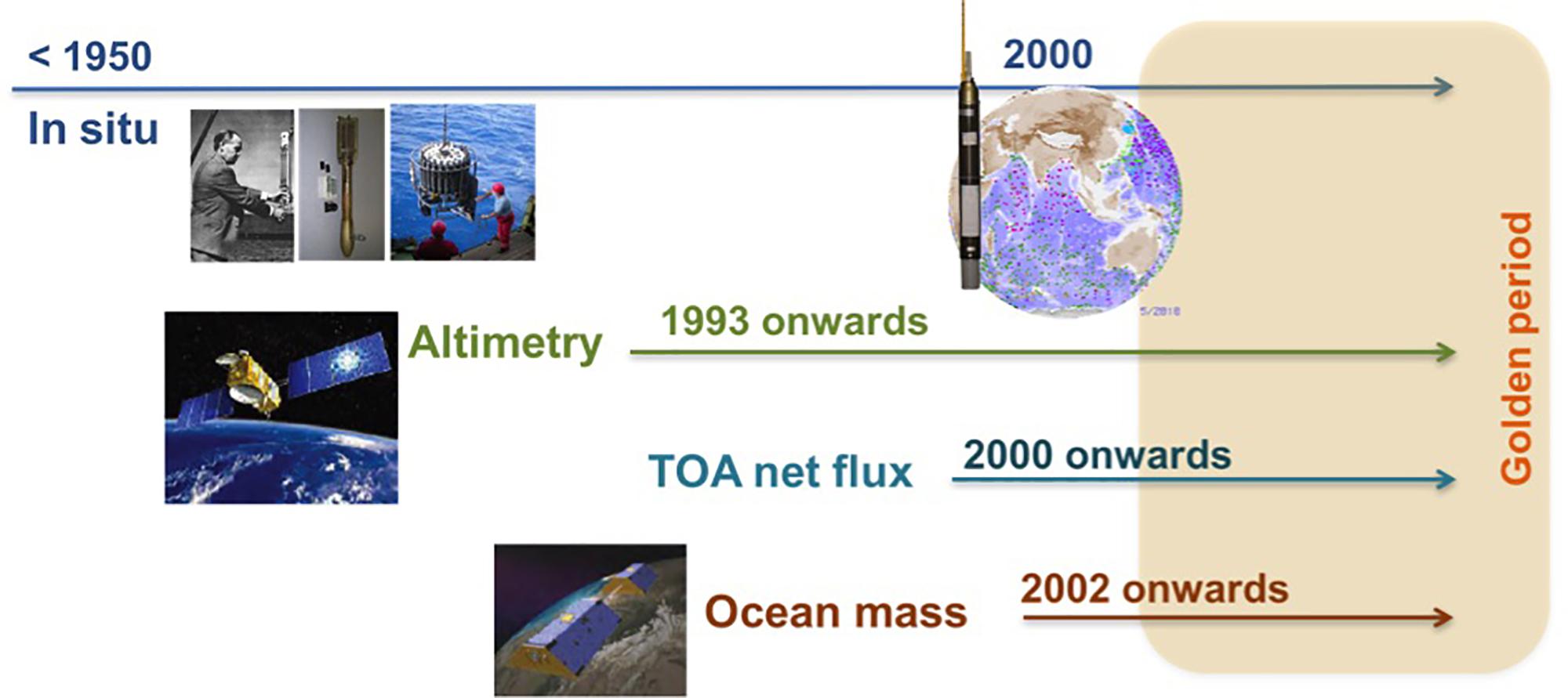
Figure 1. Schematic representation of the evolution of in situ and remote sensing observing systems for the evaluation of global ocean heat content. The shaded area indicates the so-called “golden period” of Earth system measurements for global ocean heat content estimates, which starts circa 2005 and is characterized by initially sparse but steadily improving global coverage of in situ temperature measurements through the Argo program.

The second period, which starts with satellite altimetry in 1993, includes more complementary observing systems, from remote sensing techniques, fixed stations, modern shipboard measurements and autonomous in situ platforms¹. This era also saw the development of reanalysis systems, which assimilate in situ and satellite observations into numerical models to provide a four-dimensional perspective of the global ocean (Balmaseda et al., 2013; Palmer et al., 2017; von Schuckmann et al., 2018). Storto et al. (2019) outline advances and current challenges for ocean reanalyses.

The third period, an ongoing “golden era” for OHC, is characterized by a surge in temperature measurements with near global ocean data coverage for the upper 2000 m, mainly from Argo profiling floats (Riser et al., 2016), and the availability of information for Earth energy/sea level budget constraint evaluations (Loeb et al., 2012; Llovel et al., 2014; Trenberth and Fasullo, 2016; von Schuckmann et al., 2016; Chambers et al., 2017; Dieng et al., 2017).

Estimating the Ocean Temperature From In Situ Observations

The in situ Observing System

Accurate reconstruction of OHC requires subsurface measurements that are sustained over time (decades and longer) and sufficiently widespread to adequately capture spatio-temporal changes. Evolving changes to instrumentation, geographic range and depth coverage (Figure 2) can introduce uncertainty into the determination of long-term global trends and regional patterns (Wunsch, 2016).

FIGURE 2

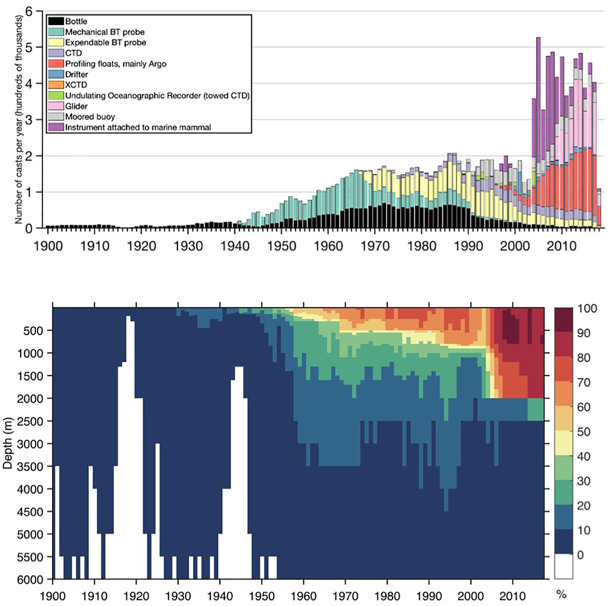
Figure 2. (Upper) Number of subsurface ocean temperature profiles per year by instrument type 1900–2017. [BT, Bathythermograph; CTD, Conductivity- Temperature-Depth; XCTD, Expendable CTD]. (Lower) Percentage (%) of data coverage for 3 × 3 boxes over the global ocean area from 5 to 6000 m.

The primary modern instruments comprising the OHC observing system since the 1940s (Figure 2) are Mechanical Bathythermographs (MBTs), Expendable Bathythermographs (XBTs), Nansen/Nisken bottles, and Conductivity-Temperature-Depth (CTD) instruments. Argo floats, gliders, ice-drifters, instrumented pinnipeds, and moored buoys often carry CTDs. Nansen or Niskin bottle hydrocasts with attached reversing thermometers and the CTD casts represent together an important portion of the global archive as they are superior in precision and provide more full-depth temperature profiles compared to other instrumentation types. Several old expeditions provided observations suitable for the estimation of long-term temperature changes along specific tracks (Roemmich et al., 2012; Gouretski et al., 2013) relative to the contemporary ocean thermal state.

Together, MBT and XBT data contribute 36% of the total ocean temperature profile data available to 2013; there are ∼2.4 million MBT (1931–2004) and 2.5 million XBT profiles (1960-present) (Boyer et al., 2013). MBTs typically go down to ∼125 – 250 m and were widely deployed from 1938 to the early 1960s (Figure 2). Shallow XBTs (e.g., T4/T6) reach 450 m, and were widely deployed during the 1970s∼1980s (Figure 2). On the other hand, deep XBTs (e.g., T7/DB) provide data to 800 m, and were widely used during the 1990s and early 2000s (Figure 2). These devices have typically been deployed from naval and research vessels and, more recently, from merchant ships of opportunity for XBTs.

The Argo Program, designed in 1998 (Argo Science Team, 1999), was transformational for OHC estimation because it enabled high-quality profile CTD data to be obtained nearly anywhere in the ocean without a human monitor present, thus reducing or eliminating coverage biases of ship-based systems. Argo first achieved its initial goal of 3000 profiling floats in November 2007. Its present coverage of about 3800 floats (Figure 3A) is close to the target of 4000, and is beginning to move into marginal seas, seasonally ice-covered regions, and increasing float density in critical areas (Jayne et al., 2017). The data coverage is >80% of the global ocean area (3 by 3 degree box) after 2007 from depth 0–1200 m and >70% for 1200–2000 m (Figure 2). Advances in profiling float technology, including bidirectional communications, have increased float lifetime and improved coverage. Argo’s near-global uniform coverage has resulted in a dramatic reduction of the uncertainty of global OHC changes and related ocean thermal expansion estimates (e.g., Domingues et al., 2008; Lyman and Johnson, 2014; Boyer et al., 2016; Cheng et al., 2016b; Johnson et al., 2018; The WCRP Global sea level budget group, 2018).

FIGURE 3

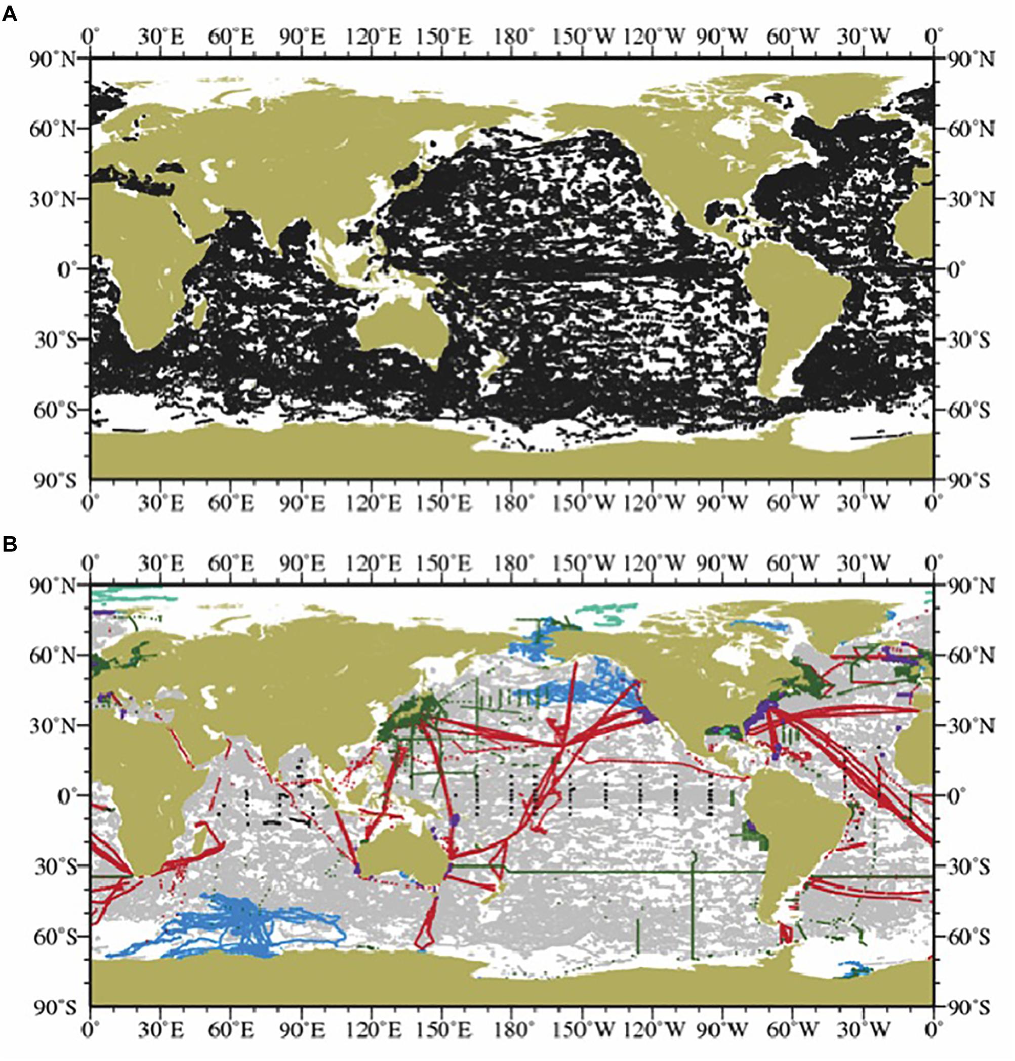
Figure 3. Temperature profile locations in 2017 from (A) Argo floats and (B) ship-based bottle/Conductivity-Temperature-Depth (CTD) casts (dark green), Expendable Bathythermographs (XBT) drops (red), tropical moored buoy daily means (black), glider cycles (purple), instrumented pinniped dives (blue) and ice-tethered profilers (light green) [Argo cycles in background (gray) for comparison].

Other instrument platforms have contributed to temperature profile data used to calculate OHC. The tropical moored buoy array, as well as moored buoys represented by OceanSITES (Figure 3B), have provided temperature measurements at specific depths across the global tropical latitudes and as point sources elsewhere. Gliders, autonomous vehicles more directly controllable than Argo floats with shorter deployment periods, have become a valuable source for CTD data with programs focused on United States coastal areas, Australian waters, and the European Union areas of interest. These platforms have the potential to contribute in a more coordinated fashion, including measurements across boundary currents. Instrumented pinnipeds may be a valuable source of CTD data from seasonal ice-bound waters and elsewhere.

Importance of Data Management

Effective management of subsurface ocean temperature information is the basis for the dissemination and reproducibility of accurate scientific knowledge of ocean warming and its causes. Effective management is also needed for timely and user-friendly access to data products and services to various community sectors (including scientists, industry, government etc.). Data management starts at the time of data collection and persists throughout the data lifecycle.

Consistent synthesis of the various data sources is crucial to ensure optimal OHC changes estimates. The optimization process includes quality control (QC) of the available data within the individual expert communities (e.g., the Global Temperature and Salinity Profile [GTSPP], for XBTs) and collectively, as well as pre-processing with any bias corrections that are necessary.

Historical ocean temperature profiles, particularly those outside expert community control such as the Argo Data Management System (ADMS) or outside highly controlled programs such as the World Ocean Circulation Experiment (WOCE) can suffer from inconsistencies in QC that can impact OHC estimation. The International Quality Controlled Oceanographic Database (IQuOD) program (Domingues and Palmer, 2015)² is filling this gap by developing internationally coordinated delayed QC standards which will be implemented in a homogeneous, structured, and fully documented form.

Calculating OHC Changes From in situ Temperature Profiles and Sources of Uncertainty

For a given depth layer, OHC is defined as the volume integral of temperature multiplied by seawater density and the specific heat capacity, with units of Joules:

$$OHC={\iiint }_{h2}^{h1}p{C}_p\mathrm{\Theta }𝑑x𝑑y𝑑z$$

Here, (following TEOS-10; IOC et al.,, 2010) ρ is seawater density, C_p is the (constant) specific heat capacity, Θ is conservative temperature (derived from in situ temperature, absolute salinity, and pressure), and h₁ and h₂ are the depth range over which the heat content is computed.

The traditional approach to estimate OHC from ocean temperature profiles involves gridding the available observations and interpolating across data gaps using a statistical mapping method (e.g., Abraham et al., 2013). Prior to the gridding of data, a seasonal climatology is usually subtracted from each profile to convert the observations into temperature anomalies with the annual cycle removed. Temperature anomalies have larger de-correlation length scales than the full temperature field and therefore provide a more useful basis for mapping and interpolation. A reliable mapping method should provide a good estimate of signal and error while minimizing sources of uncertainty.

Ocean heat content trends are sensitive to the choice of statistical model for the mapping, which may include both a least squares fit (e.g., to estimate the annual climatology to be removed from the data) and objective mapping of residuals. For the Argo period, including a climatological trend in the least squares fit results in smaller biases and larger long-term changes in OHC (Domingues et al., 2008). Objective mapping is the most common statistical approach used to map the residuals, although details on how it is implemented differ among groups (e.g., Levitus et al., 2000, 2012; Willis, 2004; Ishii and Kimoto, 2009; Good et al., 2013; Cheng et al., 2014, 2017; Ishii et al., 2017; Kuusela and Stein, 2018). The approach can evolve over time within the same group (e.g., Lyman and Johnson, 2008; Lyman et al., 2010). Modeling the time dimension in objective mapping yields smoother month-to-month transitions and smaller overall uncertainty in OHC changes. Estimating space-varying decorrelation scales from observations is key to quantifying uncertainty (Kuusela and Stein, 2018). Other approaches to mapping include simple grid box averaging (e.g., Palmer et al., 2007; von Schuckmann and LeTraon, 2011; Gouretski, 2012, 2018) or reduced-space optimal interpolation (Domingues et al., 2008; Church et al., 2011). Boyer et al. (2016) estimates an uncertainty of ±1 Wm^–2 annually for 1970–2008 due to mapping method differences. Lyman and Johnson (2008), Cheng and Zhu (2014a), and Durack et al. (2014) noted that estimates of OHC trends from many mapping methods are biased, because the mapping methods tend to relax toward the climatological values in the data gaps. As data increase with time, the uncertainty due to mapping is reduced and OHC estimates from different groups show more consistency (Johnson et al., 2018). Nevertheless, understanding of the performance of the mapping methods and improving them are the major step forward to reduce the uncertainty in OHC estimate.

Lyman and Johnson (2014) shows that the observed temperature profiles can be integrated in depth first for OHC calculation, which reduces the dimensionality of the (mapping) problem, as well as reducing uncertainty due to modeling the vertical dimension. Cheng and Zhu (2014b) show that using different interpolation schemes can lead to small differences in OHC calculation, because of the insufficient vertical resolution in the old observation records.

In 2007, it was discovered that systematic errors in XBT and MBT data significantly impacted the accuracy of OHC changes (Gouretski and Koltermann, 2007), creating a spurious “hump” in the OHC record during the late 1970s to the early 1980s (Bindoff et al., 2013). Since then, multiple methods have been proposed to correct biases in XBT data (Cheng et al., 2016a, 2018). By applying six correction schemes for OHC calculation separately and after calculating the standard deviation among the obtained OHC time series, Boyer et al. (2016) found that the uncertainty in OHC due to XBT error is 0.5 – 1.1 Wm^–2 annually for 1970–2008 and 0.7 – 1.4 Wm^–2 annually for 1993–2008, depending on the mapping method. Since 2014, the community has recommended the Cheng et al. (2014) method as the most complete correction for XBT data for calculating OHC changes; it accounts for all of the known factors that influence XBT error. Consequently, the uncertainty in OHC changes due to XBT error is expected to be smaller than that shown in Boyer et al. (2016). For example, the mean standard deviation of the best two schemes (Levitus et al., 2009; Cheng et al., 2014) identified in Cheng et al. (2018) is only 0.2 Wm^–2 annually for the 1970–2004 period (Cheng et al., 2018). XBTs are now a much smaller part of the overall observing system than in the pre-Argo time period, with corresponding smaller uncertainty contribution.

As stated above, in general, OHC changes are computed by using ocean temperature anomalies (residuals) relative to a baseline climatology. In some cases, the selected climatology affects OHC changes estimates and quality control results (Ishii and Kimoto, 2009; Lyman and Johnson, 2014; Cheng and Zhu, 2015; Boyer et al., 2016, 2018). Several centers adopt objective analysis as a global mapping method, and some types of this method yield temperature values close to the climatology particularly in data-sparse regions. Uncertainty due to baseline climatology ranges 0.2–0.9 Wm^–2 for the six mapping methods in Boyer et al. (2016). The quality of climatology is not uniform in space because of the spatio-temporal data sampling density and observational biases like those in XBT observations. Temperature biases for XBTs tend to be larger around the thermocline and at greater depths (Gouretski and Reseghetti, 2010; Cheng et al., 2018). Furthermore, the climatological baseline of ocean temperatures has temporally been changing due to global warming. To obtain reliable OHC changes over 60 years or more is equivalent to understanding acceptable climatological mean fields of ocean temperature before the Argo era. Reconstructing high-quality ocean observations is key to solving this.

In summary, each of the available observational OHC changes estimates is affected to different extents by uncertainties due to specific systematic instrumental adjustments, to baseline climatology from which the anomaly is calculated, and data distribution irregularity (mapping). These errors are not independent, therefore, it is still difficult to fully isolate them and quantify their contributions separately. Further actions and novel methods are needed to tackle this problem.

Present and Future Observational Coverage

A key to reducing uncertainties in OHC changes is the flow of high quality observations to researchers making the calculations. Many elements of the Global Ocean Observing System routinely take ocean temperature profiles (Figure 3), including the Argo profiling float program, the XBT network, GO-SHIP, OceanSITES,regular national hydrographic surveys, and the activities of short-term research campaigns (crosslink to Palmer et al., 2010). These observations vary in accuracy and many have been northern-hemisphere focused. A step-change in our ability to monitor the upper OHC came with the implementation of the global Argo program (Figure 2). Delivering a profile nominally every 3° lat. × 3° long every 10 days (Jayne et al., 2017), the nearly global reach and high quality of Argo temperature and pressure observations allow mapping heat content patterns on roughly seasonal and 1000 km scales in the ice-free open ocean.

Argo’s revolutionary impacts on basic research, climate assessment, ocean reanalysis and forecasting, and education are widely recognized. Nevertheless, Argo’s future includes major organizational and technical challenges. Major enhancements to Argo, including Deep and Biogeochemical Argo must be implemented with new resources and without eroding Core Argo. The successful ADMS must continue responding to new requirements in ways that do not overwhelm data managers. International protocols for floats drifting into Exclusive Economic Zones (EEZs) must be broadened to simplify float deployment in these regions. The supply chain for Argo floats and sensors must be made robust against sole-source failures. The mean lifetime of Argo floats, presently >4 years, should be extended further through design improvements, analysis of long-term failure modes, and adoption of improved battery technologies. Argo’s leadership model must prove capable of spanning scientific generations while preserving its focus, originality, and collaborative nature. Finally, Argo’s role as an inter-dependent element of the integrated observing system requires that all elements thrive together.

Diversity in sensors and platforms are essential to help build confidence in the OHC record, particularly for tracking the small but persistent global ocean warming signals. With its present dependence on one sensor manufacturer, Argo is highly vulnerable to manufacturing errors. GO-SHIP and OceanSITE records, which are post calibrated and of high quality, are essential points of cross-reference for Argo. Satellite altimeter data are also used to identify and remove suspect Argo data. XBT lines give an insight into scales of variability not resolved by Argo, particularly near the margins of the open oceans. In this way, a robust OHC observing system involves a mixture of platforms to ensure robustness and confirmation of signals observed across networks.

Boundary currents (eastern and western as well as northern and southern currents in closed basin) are not fully represented by Argo as the core floats have a parking depth of 1000 m and therefore they do not sample waters located in the upper 1500 m of every continental slope (that represent an important fraction of boundary currents). Also, Argo floats swiftly pass through the energetic regions. Ocean analyses at present have limited capability to identify the mesoscale variability among boundary current (WBC) and Antarctic Circumpolar Current (ACC) regions which could induce an inverse cascade of kinetic energy and affect the large scale low-frequency variability (Penduff et al., 2018). Inter-comparison among three available ocean analyses (EN4, Ishii and IAP dataset) revealed a large spread of OHC change in the WBC and ACC regions: >10 × 10⁸ J m^–2 even during the Argo era (2005–2012), 2–10 times larger than the open ocean regions (Wang et al., 2018). Removal of WBC and ACC regions reduces the spread of global integrated OHC change estimates in the upper 1500 m by 13% during 1976–2012, despite these regions small (∼6%) portion of the global ocean. Within these regions, the root-mean-squared error (RMSE) of OHC tendency could be larger than 100 Wm^–2 locally (i.e., with respect to the local surface and not with respect to the global surface at TOA, Wang et al., 2018), which has the same magnitude as the climatology mean net air-sea heat flux (Liang and Yu, 2016). The large error among these regions is partially because the calculation of tendency from a noisy time series exacerbates the noise. Therefore, advanced ocean observing systems in the WBC and ACC regions are required to better resolve mesoscale and sub-mesoscale variability and aid in higher resolution ocean analysis. Complementary to Argo, high-resolution XBT casts, gliders under pre-set routines, as well as mooring networks such as the North Pacific Ocean Circulation Experiment (NPOCE) (Wang and Hu, 2010) could reduce the uncertainty of OHC change estimates.

It has always been difficult to obtain subsurface ocean temperature measurements in the Arctic, leading to a dearth of historic and recent data (Zweng et al., 2018). In 2017, there were subsurface temperature data from only three research cruises north of 66°N generally available through the World Ocean Database, down from 12 in 2016. There are some Argo floats at high northern latitudes, mainly in the Greenland-Iceland-Norwegian seas (GIN) area. Argo floats are more prevalent at southern high latitudes, including some with ice-sensing technology (Riser et al., 2018). The only regular subsurface temperature measurements presently gathered in the high Arctic (>80°) are from the Ice Tethered Profiler (ITP) program (Toole et al., 2011). A rough estimate of OHC difference between the 1955–1964 and 2005–2012 periods using decadal mean temperature fields from the World Ocean Atlas (Locarnini et al., 2013) shows ∼4% of global OHC change occurred in the Arctic (including GIN Seas and Baffin Bay). Coverage in the Russian Arctic and high Arctic was actually better in the 1955–1964 period. Sustaining the ITP program, purposeful planning of Arctic cruises, better global data exchange, and extending Argo can close the data gaps in the Arctic. Sustaining Southern Ocean Argo, increasing deployment of under-ice Argo floats, and utilization of quality pinniped mounted sensors can help close the data gaps in the Southern Ocean.

It is also difficult to obtain subsurface ocean temperature measurements in EEZs. A ∼ 0.1 Wm^–2 increase between 1955–1964 and 2005–2012 (calculated as above for the Arctic) is found for the Tropical Asian Archipelago (TAA) and the Andaman Sea, or slightly less than 2% of the total +6.5 Wm^–2 increase calculated from the same mean fields. A similar rough estimate for non-TAA continental shelf/coastal areas adds another ∼1.5% OHC change in shallow areas not presently well sampled by Argo. While shelf OHC changes can be important regionally (e.g., Forsyth et al., 2015; Turner et al., 2017) they constitute only a small percentage of global change. Some semi-enclosed ocean areas such as the Mediterranean and the Gulf of Mexico are sampled by Argo and other systems. Others, such as the Sea of Okhotsk have almost no available data for the last 10 years. Argo extensions and the systematic deployment of gliders can add reliable data collection in marginal seas.

The ocean below 2000 m has warmed significantly since the 1990s, accounting for ∼10% of the total ocean heat uptake (Purkey and Johnson, 2010; Rhein et al., 2013; Desbruyères et al., 2016). Recent estimates of the deep OHC change are based on decadal repeats of coarse hydrographic sections (Talley et al., 2016) and the only statistically robust deep OHC trends are basin-wide, decadal averages owing to limited data (Figure 2). Nonetheless, a spatially coherent global picture has emerged of an intensified deep warming, originating from deep water formation sites in the Southern Ocean and propagating through the Meridional Overturning Circulation, with a statistically significant contribution to the global ocean heat uptake.

The global deep (below 2000 m) and abyssal (below 4000 m) OHC accumulation rates between the 1992 and 2009 are 0.04 (±0.05) Wm^–2 and 0.02 (±0.01) Wm^–2, respectively, and local estimates show large spatial variability (Figure 4; updated from Purkey and Johnson, 2010). The Southern Ocean below 1000 m has warmed 10 times faster than elsewhere in the deep ocean. While there has been some regional variability, the total deep-ocean warming rate has not changed outside the error bars over the past 3 decades (Lyman and Johnson, 2014; Desbruyères et al., 2016).

FIGURE 4

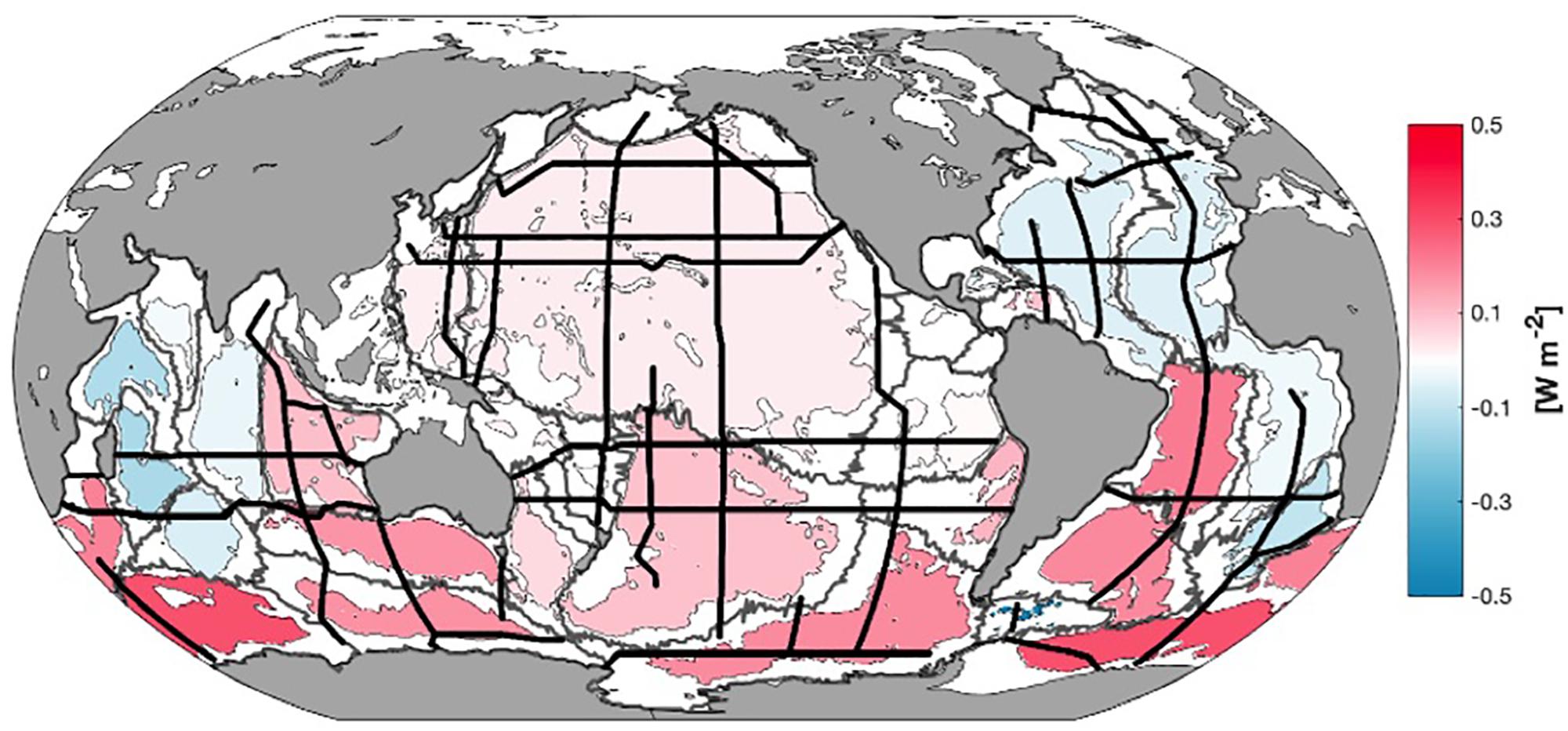
Figure 4. Heat flux (colors) through the 4000 m isobath (thin gray lines) needed to account for the mean local basin (thick gray lines) abyssal ocean warming estimated from GO-SHIP full depth hydrography sections occupied two or more times (black) between 1981 and 2018. Methods follow Purkey and Johnson (2010) with warming rates updated through 2018.

Continuous, global, top-to-bottom ocean temperature data are needed to monitor the deep OHC change. Plans are underway to make it possible through the implementation of the new Deep Argo array, capable of sampling the water column down to 6000 m (Roemmich et al., in review). The envisioned 5° lat. × 5° long. × 15-day Deep Argo array with highly accurate temperature and pressure standards (0.001°C and 3 dbar, respectively) would decrease errors in decadal deep OHC trends to ±0.006 Wm^–2, compared to ±0.04 Wm^–2 uncertainty based on present observing systems (Johnson et al., 2015). Deep Argo will complement the ongoing decadal repeat hydrography (Sloyan et al., in review) and existing deep moorings (Cronin et al., 2012). In addition, new technologies, including deep-gliders that operate to 6000-m depth, are under development to bridge gaps in deep-ocean temperature observations in boundary regions (Eriksen, 2017).

Time Scale of OHC Estimates

When estimating the uncertainty in OHC changes on decadal time scales, ideally all sources of uncertainty explained above should be taken into account and combined. This is difficult because the in situ observing system and therefore the different sources of uncertainty change with time and space. Some sources of uncertainty may include spatial and temporal correlation adding to the complexity of the calculation. Different groups have elaborated different strategies to calculate OHC trend uncertainties. In Table 1 we show the most recent estimate of the uncertainty in OHC trends over the last two decades from in situ data and recall the different sources of uncertainty they take into account. Because different groups account for different sources of uncertainty, their total uncertainty estimates differ substantially. However, in general, for uncertainty estimates over recent periods (estimates starting in 1993 or in 2005), the time and space error correlation and the error due to the data distribution in time and space appear to be the most important terms (see Table 1). Here after (e.g., Table 3), we consider the uncertainty estimate based on work by Johnson et al. (2018) for the in situ based estimates of OHC trends, because it is the most comprehensive estimate considering OHC over the full 0–2000 m ocean column and covering both the altimetry period (1993 onwards) and the Argo period (2005 onwards, see Table 1). We apply a least square method to the average of the four time series used in Johnson et al. (2018) weighted by the square sum of the four associated standard errors in order to estimate the trend. In the trend uncertainty calculation, degrees of freedom are adjusted taking into account the temporal correlation of the residuals following Johnson et al. (2018). This yields an uncertainty of ±0.11 Wm^–2 for the OHC changes over 2006–2015. The result is given in Table 3. This uncertainty does not take into account the uncertainty due to data distribution, which may amount to ∼0.1 Wm^–2 (see Table 1).

TABLE 1

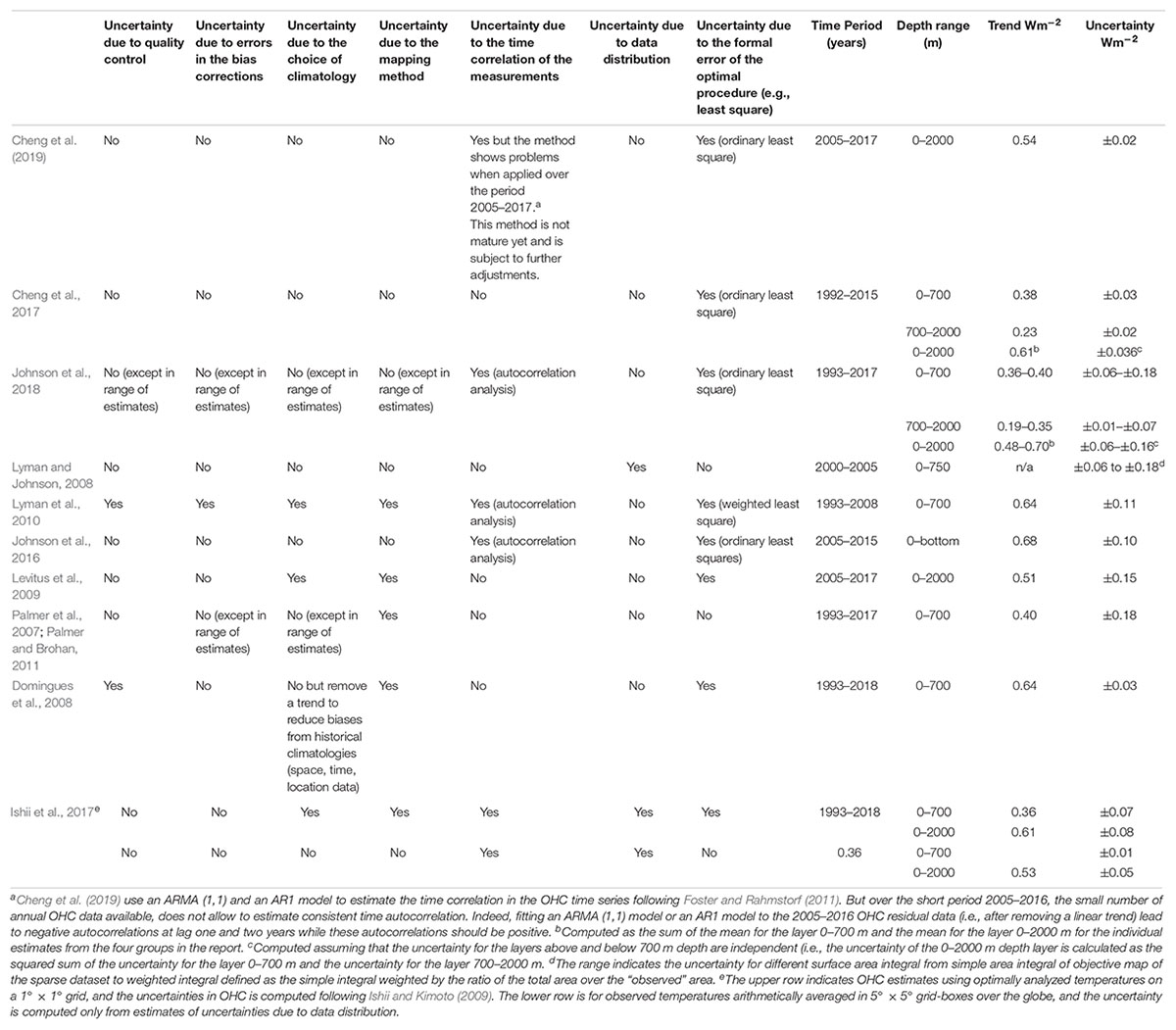
Table 1. Ocean heat content change in Wm^–2 and associated uncertainties from recent studies based on in situ data. Column 2–8 indicate the different sources of uncertainty accounted for. Column 9 indicates the period of computation. Column 10 indicates the region that is considered.

TABLE 2

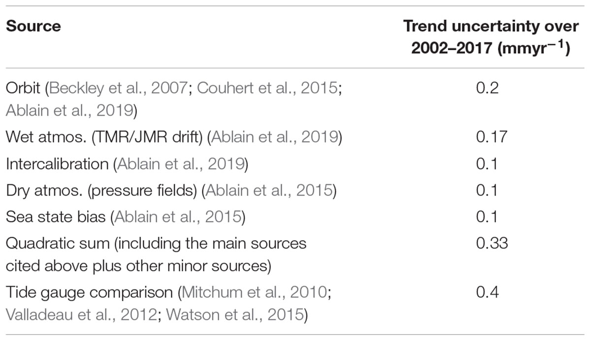
Table 2. GMSL trend uncertainties (in mmyr^–1) over 2002–2017 estimated from the error budget approach and from the comparison with tide gauge records.

TABLE 3

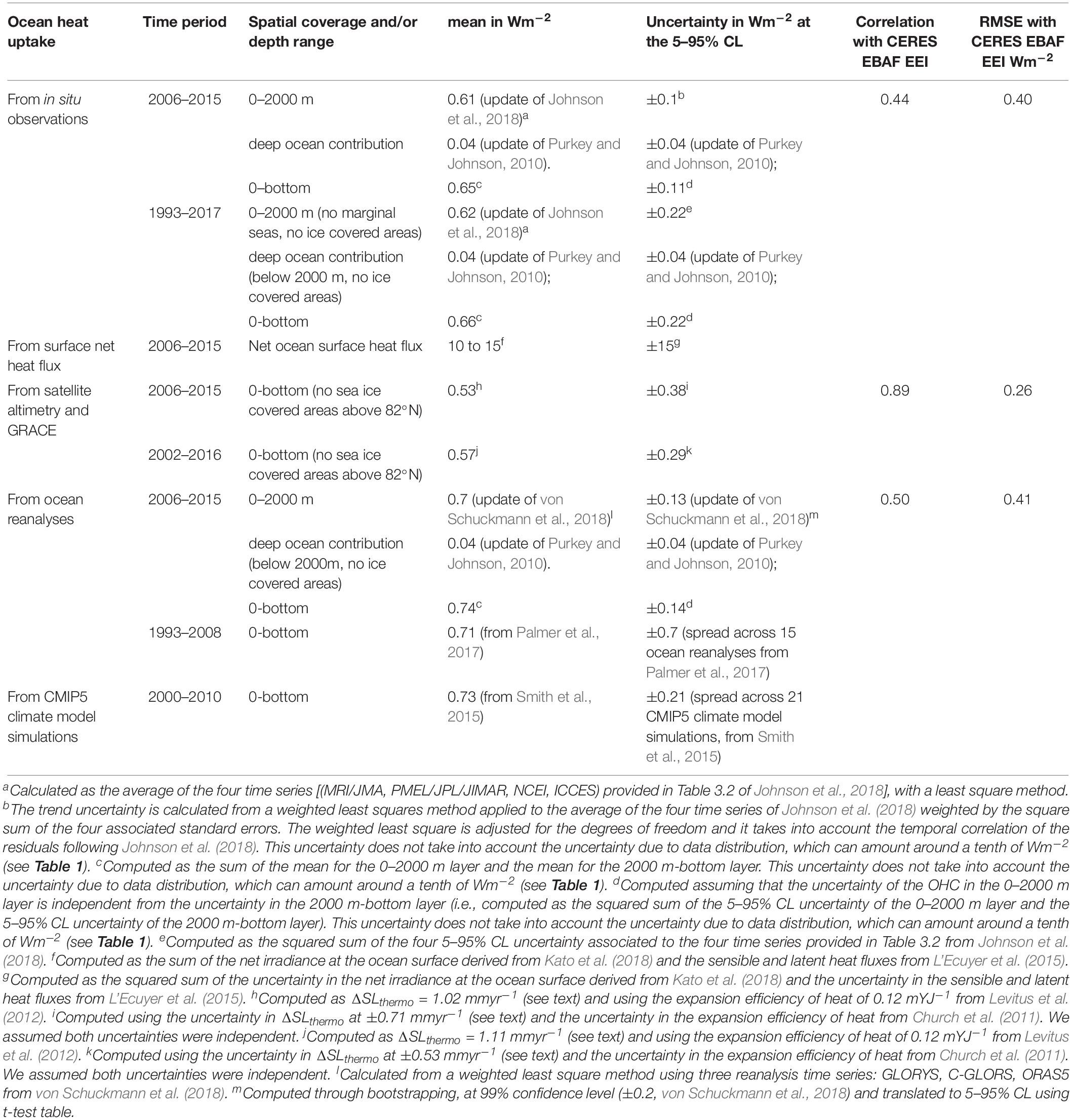
Table 3. Ocean heat uptake and associated uncertainty as estimated with the different methods listed in this paper. The correlation and the RMSE with the TOA radiative budget estimate of the EEI from CERES EBAF is given in column 6 and 7. CERES EBAF values taken from Johnson et al. (2016). All with respect to global surface.

Estimating the uncertainty in OHC changes at interannual time scales is more challenging because of insufficient spatio-temporal coverage. So far, few studies have provided estimates. Estimates of annual OHC changes for 0–2000 m have standard errors of 0.3–0.6 Wm^–2 over the Argo era, and those errors increase substantially for the pre-Argo time period (Johnson et al., 2018, their Figure 2). Thus, while year-to-year variations in global OHC change during the Argo time period may be well correlated with El Niño indices and TOA radiative imbalance variability, the interannual signal does not quite rise above the uncertainties in the estimates, and monthly estimates from in situ ocean observations alone are much noisier (Johnson and Birnbaum, 2017).

Monthly estimates of global OHC for 0–2000 m exhibit variability several times that of TOA satellite estimates (Johnson and Birnbaum, 2017, their Figure 1B) and are not yet useful for the study of EEI when made from ocean temperature observations only (Trenberth and Fasullo, 2016). Nonetheless, the seasonal cycle is well resolved by observations at monthly time-scales when using data from several years (Roemmich and Gilson, 2009), and even more so now with more than a decade of Argo data³.

A New Technique to Monitor Global OHC Changes: Internal Tide Oceanic Tomography

Review of the Concept, Advantages, and Challenges

A new concept of internal tide oceanic tomography (ITOT) was recently proposed to monitor global OHC changes (Zhao, 2016). ITOT detects OHC changes by measuring travel time changes of long-range internal tides. The underlying principle is that upper ocean warming strengthens ocean stratification and thus increases the propagation speed of internal tides. ITOT is similar to ocean acoustic tomography but that the work waves are internal tidal waves. Acoustic tomography was brought up about 40 years ago to detect ocean temperature changes from travel time changes of acoustic waves (Munk and Worcester, 1976; Munk et al., 1995; Dushaw, 2018, Howe et al., 2019). The two tomographic techniques have the same advantages: they suppress the temperature perturbations caused by mesoscale processes (major error sources in field measurements) and measure basin-scale OHC changes (compared to station-wise measurements). Therefore, the tomographic techniques may complement the currently existing in situ ocean profile technique described above (Dushaw, 2018).

ITOT monitors OHC changes by tracking long-range propagating internal tides. Internal tides are generated in tide-bottom interactions over topographic features. Low-mode internal tides may travel hundreds to thousands of kilometers. Internal tides have cm-scale sea surface height (SSH) fluctuations, which can be detected by satellite altimetry. Figure 5 shows the global mode-1 M2 internal tides from 20 years of satellite altimeter data. The internal tide field has been separated into northbound and southbound components. The separation makes it possible to track the long-range propagation of each internal tidal beam and estimate OHC changes. Figure 5 shows that long-range internal tidal beams are widespread in the Pacific, Atlantic, and Indian Oceans. ITOT can track M2, S2, O1 and K1 internal tides, and for each tidal constituent both mode-1 and -2 waves. The multi-constituent, multi-mode method has a much better spatial coverage of the global ocean. Internal tides are powered by the astronomical tidal potential, and thus no cost is needed to maintain their radiation sources. ITOT has a relatively low temporal resolution, due to long repeat cycles of satellite altimetry. Therefore, ITOT may offer a long-term low-cost observing network.

FIGURE 5

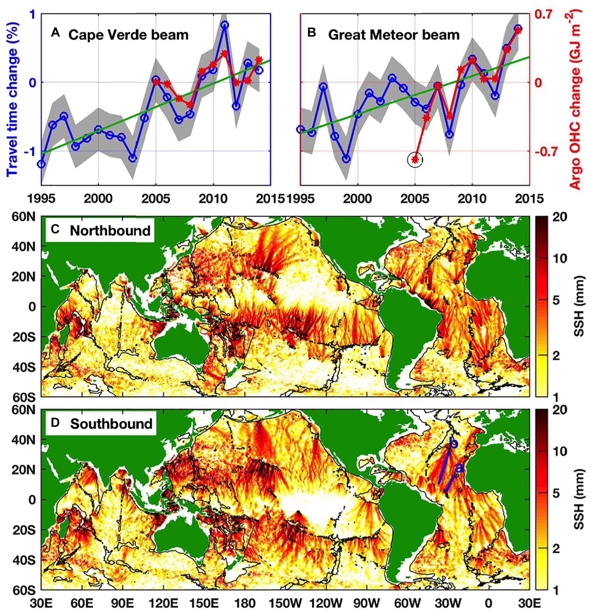
Figure 5. Internal tide oceanic tomography. (A,B) Travel time changes in percentage during 1995–2014 along mode-1 M2 internal tidal beams from (A) Cape Verde Islands and (B) Great Meteor Seamount. See panel (D) for beam locations. Both beams reveal significant interannual variations and bidecadal trends in the travel time change. Argo-measured OHC changes are overlapped with a conversion rate of 1% versus 0.7 GJ/m2 as explained in the text. (C,D) Global mode-1 M2 internal tides from 20 years of satellite altimeter data. The northbound (propagation direction ranging 0°–180°) and southbound (180°–360°) components have been separated. OHC changes can be monitored by tracking long-range internal tidal beams.

Much work is needed to develop ITOT from a proof-of-concept level to a mature level. There are two major challenges. The first challenge is how to precisely measure the phase of internal tides by satellite altimetry. It stems from the complex nature of the internal tide field and the low spatio-temporal sampling rates of altimeter satellites. The current-generation nadir-looking satellite altimetry samples the ocean along sparse ground tracks with time intervals of O (10) days. To resolve spatio-temporal variations of internal tides, time series of 1 year or longer are needed, depending on the number of satellites in the constellation. Uncertainties in the speed changes may be caused by background currents and salinity anomalies. They can be evaluated using overlapping internal tidal beams and/or in situ measurements. The second challenge is to derive OHC changes from the speed changes of internal tides. ITOT itself cannot distinguish the upper- and lower-layer contributions. The ambiguity requires constraints from in situ measurements. Heat enters the ocean from the sea surface and is redistributed in the ocean interior. Ocean warming can be approximated using Argo and shipboard measurements. It generally follows a baroclinic profile—more heat is stored in the upper layer (Levitus et al., 2012). Assuming that ocean warming follows a normalized profile, its magnitude can be computed from travel time changes of internal tides. In the North Atlantic, about 0.7 GJm^–2 is required to increase the internal tide’s phase speed by 1%. The spatially varying conversion rate can be determined using available in situ measurements and internal tide dynamics.

The propagation of two southbound mode-1 M2 internal tidal beams in the North Atlantic has been studied (Figure 5). For each beam, the annual travel times are calculated from the phase increase along the beam. The travel time change rates (in percentage) demonstrate significant inter-annual variability, compared to its 5–95% confidence intervals (shading). Bidecadal trends are obtained by linear fit (green lines). Both beams reveal that their travel times decreased by about 1% over the past two decades. The propagation is about 1–2 h faster, suggesting that this part of the North Atlantic is getting warmer. Argo measured along-beam-mean OHC changes are calculated and overlapped in Figure 5. The ITOT estimates and Argo measurements agree well for both interannual variations and bidecadal trends. This example confirms that ITOT is feasible and reasonable.

Gap Analysis of the Current Measurement Capacity and Ways for Improvement

Currently there are about 25 years of satellite altimeter data since 1993 made by a series of altimeter missions. The dataset is long enough to study interannual variations and bidecadal trends in the global OHC. ITOT can be used to analyze 3 years of GeoSat data from 1986–1989 to retrieve OHC changes in the 1980’s. In the next 5 years, there will be a few new altimeter missions in operation including Jason classes, Sentinal-3 series, HY-2 series (Haiyang-2, Dong et al., 2004), and GFO-2 (Geosat Follow-On-2, Benveniste, 2011). The combination of these satellites will maintain the measurement capability of ITOT at the present level.

In the next 5–10 years, the two major challenges of ITOT may be addressed, leading to improvements of ITOT’s measurement capability. First, the next-generation wide-swath altimetry (such as SWOT -Surface Water and Ocean Topography, Morrow et al., 2019- and COMPIRA -Coastal and Ocean Measurement mission with Precise and Innovative Radar Altimeter, Uematsu et al., 2013) will measure high-resolution SSH in the real two-dimensional ocean. In contrast, the conventional nadir-looking altimetry has low spatial resolution. Wide-swath altimetry will greatly improve our capability of mapping internal tides and their propagation speed. Second, the ITOT derived OHC changes will be calibrated against other OHC estimate techniques. In addition, the ECCO2 state estimate (Estimating the Circulation and Climate of the Ocean, Phase II, Menemenlis et al., 2005) can be used to directly calculate the internal tide’s speed and OHC changes, so that ECCO products can be used to assess the accuracy of ITOT. In particular, acoustic tomography has been conducted in a series of field experiments (Dushaw et al., 2009). It will be very useful to compare the OHC changes estimated by the two tomographic techniques.

Estimating the Ocean Surface Net Flux From Space Observations

Because energy storage in the atmosphere over time scales longer than a year is two order of magnitude smaller than heating rate of the ocean (Church et al., 2011), the global annual mean net surface flux is in principle nearly equal to the TOA irradiance. Thus TOA irradiance can in principle be used to estimate the ocean heating rate. The flux components needed to compute the net surface flux are radiative flux, turbulent flux, and flux associated with mass transfer. In the following sections, we provide brief descriptions of algorithms to estimate surface fluxes and uncertainties in the fluxes derived from the algorithms.

Radiative Flux

Radiative fluxes (irradiances) at the ocean and atmosphere boundary are estimated by radiative transfer models. These models are based on radiative transfer theory and solve an integro-differential equation of radiative transfer typically with a two- or a four-stream approximation. Polarization state is neglected. Primary inputs to the radiative transfer model are height dependent atmospheric temperature and water vapor mixing ratio, cloud and aerosol properties, ocean surface albedo and emissivity. Satellite observation-based estimates generally take temperature and humidity from reanalysis data products. Physical and optical properties of clouds and aerosols are estimated from satellite observations either passive sensors (e.g., imagers like Moderate Resolution Imaging Spectroradiometer (MODIS), Visible Infrared Imaging Radiometer Suite (VIIRS), and imagers on geostationary satellites) or active sensors [e.g., Cloud-Aerosol Light Detection and Ranging (LIDAR) with Orthogonal Polarization and Cloud Profiling Radar on CloudSat]. Cloud properties include cloud top and base heights, optical thickness, and particle size and water phase. When passive sensors are used to retrieve cloud properties, the cloud top height is estimated from the effective cloud top temperature combined with the vertical temperature profile. Passive sensors cannot observe the cloud base height directly. It is usually estimated empirically with the combination of the cloud optical thickness and cloud top height. Active sensors can directly detect cloud top and base heights. In additions, the vertical profile of particle size and phase can be derived from their observations. Once particle size and phase are derived, wavelength dependent extinction coefficient, single scattering albedo and asymmetry parameter are determined theoretically by assuming cloud particle shape. Spherical particles are assumed for warm clouds and their optical properties are computed with Mie theory. Various shapes are used for ice clouds. However, as long as the same ice crystal shape is used in both the cloud retrieval algorithm and surface irradiance computations, the error is generally small (Loeb et al., 2018b).

Similar to cloud properties, aerosol optical properties are determined from observations. Aerosol optical thickness can be derived from passive sensors and active sensors. Passive sensors can provide optical thickness at various wavelengths. Particle size is estimated from the wavelength dependent optical thickness. LIDAR that measure the backscatter extinction need to assume the ratio of the backscatter extinction and extinction coefficient to derive aerosol optical thickness. The wavelength dependent aerosol optical thickness (as well as depolarization ratio for the case of LIDAR) combined with geolocation is used to determine aerosol types. Once aerosol type is determined, wavelength dependent optical thickness, single scattering albedo, and asymmetry parameters are determined by assuming particle shape and size distribution. Wavelength dependent refractive indices of pure substances or those based on laboratory measurements are used to compute aerosol optical properties.

Surface albedos and emissivity also depend on wavelength. Ocean surface albedo (Cox and Munk, 1954; Jin et al., 2004) and emissivity (e.g., Sidran, 1981; Masuda et al., 1988) can be derived from models with relatively small uncertainty.

All inputs discussed above are used in a radiative transfer model to compute radiative flux. Diurnal cycle of temperature and humidity and cloud and aerosol properties need to be known to compute diurnally averaged radiative fluxes. Reanalysis data products provide the diurnal cycles of temperature and humidity. The diurnal cycle of clouds can be derived from geostationary satellites. An aerosol transport model (e.g., Collins et al., 2001) can be used for estimating the diurnal cycle of aerosols.

All assumptions and approximations made in deriving input variables and in the radiative transfer model introduce errors in irradiances. The uncertainty is reduced when TOA irradiances derived from observations are used to constrain the surface irradiance. Shortwave irradiances can be well constrained while constraint on longwave irradiance is somewhat weaker (Ellingson, 1995; Kato et al., 2018).

Radiative fluxes observed at limited ocean and land sites are used to evaluate computed radiative fluxes. Comparisons reported by Kato et al. (2018) show that surface monthly mean downward fluxes agree with observations to within 5 Wm^–2 for shortwave fluxes and 2 Wm^–2 for longwave fluxes when the differences are averaged over 46 ocean sites. In addition, the correlation coefficient of deseasonalized anomalies of computed and observed monthly mean regional fluxes (with the annual cycle removed) is greater than 0.94 over ocean for both shortwave and longwave radiative fluxes (Kato et al., 2018). These comparison results are used to determine the uncertainty in the net radiative flux over ocean. The uncertainty in the annual mean irradiance over the global ocean is significantly smaller than the uncertainty in the regional mean irradiance because of partial cancelation of spatially random errors. Once errors in all radiative flux components are assumed to be independent, the uncertainty in the global annual mean radiative flux over the ocean is 8.7 Wm^–2. Similarly, with the assumption of independent errors among all surface irradiance components, the uncertainty estimated by L’Ecuyer et al. (2015) for land and ocean combined leads to the global mean surface net irradiance uncertainty of 8.3 Wm^–2. The same assumption applied to the uncertainty estimated by Wild et al. (2014) leads to 7.0 Wm^–2 uncertainty in the global annual mean irradiance over the ocean. Uncertainties in the surface irradiances at different temporal and spatial scales are given in Kato et al. (2018).

Turbulent Fluxes

With the assumption of no Coriolis force and no adiabatic heating by radiation, the sensible heat, latent heat, and momentum vertical fluxes that are assumed to be uniform within the lowest atmospheric layer can be expressed as a function of temperature, water vapor mixing ratio, and wind speed scaling parameters (Monin and Obukhov, 1954). The scaling parameters, which are independent of height, are a product of a height dependent non-dimensional number that is a property of medium and height dependent temperature, mixing ratio, and wind speed. Based on this theory, turbulent fluxes are estimated using parameterized form of vertical energy transfer. One of popular algorithms is the Coupled Ocean-Atmosphere Response Experiment (COARE) algorithm (Fairall et al., 1996, 2003). The COARE bulk parameterization expresses the sensible and latent heat fluxes as a product of the density of dry air, transfer coefficient, wind speed relative to the sea surface, temperature or water vapor mixing ratio difference, and thermodynamic constant. The difference is expressed the value at the surface and at the reference height. The transfer coefficient is a product of the non-dimensional numbers that are used to express the scaling parameters.

Turbulent fluxes in the algorithm are composed of various terms that are needed to account for corrections. Although the inclusion of the sensible heat flux associated with mass transfer depending on the data product, as discussed in Fairall et al. (1996), the sensible heat flux associated with precipitation and water vapor evaporating from the ocean surface is computed by the COARE algorithm. The reference temperature used for these flux estimates is the sea surface skin temperature. In addition, an additional correction is applied to the latent heat flux estimate to account for the upward mass flow associated with non-negligible mean vertical velocity (Webb et al., 1980).

Uncertainty in turbulent fluxes are caused by the uncertainty in the transfer coefficient and in the temperature, water vapor mixing ratio, and wind speed used for the input to the algorithm. Approximately, a 10% uncertainty in the transfer coefficient used in the bulk formula results in a 10 Wm^–2 uncertainty in the latent heat flux under a tropical condition (Fairall et al., 1996). The overall error in the flux estimated by the COARE algorithm for wind speeds <10 ms^–1 is less than 5% and for wind speeds between 10 ms^–1 to 20 ms^–1 is less than 10% (Fairall et al., 2003). In addition, Andreas (1992) shows that sea spray, which is generally not considered in turbulent flux algorithms, contributes the sensible and latent heat fluxes over ocean, especially when the wind speed exceeds 10 ms^–1. The uncertainty in the global annual mean fluxes (land and ocean combined) estimated by L’Ecuyer et al. (2015) is 7 Wm^–2 for the latent heat flux and 5 Wm^–2 for sensible heat flux. The uncertainty in the global annual mean latent and sensible heat fluxes over the ocean estimated by Wild et al. (2014) is, respectively, 15 Wm^–2 and 7 Wm^–2.

Role of the Surface Net Flux Approach

If we simply average uncertainties in the global annual mean irradiance discussed above, the result is an 8 Wm^–2 uncertainty. Similarly, averaging the sensible and latent heat uncertainty of Wild et al. (2014) and L’Ecuyer et al. (2015) discussed above leads to an uncertainty of 11 Wm^–2 in the latent heat flux and 6 Wm^–2 in the sensible heat flux. If errors in these flux components are independent, the uncertainty in the global annual mean net surface flux over the ocean is 15 Wm^–2. The uncertainty in the surface fluxes is, therefore, approximately three times larger than the uncertainty in the TOA net irradiance derived from CERES observations (see the introduction and Loeb et al., 2009). In addition, when the global annual mean surface energy budget is computed from satellite-based data products, there is a significant residual of 10–15 Wm^–2 (Kato et al., 2011; Stephens et al., 2012; Loeb et al., 2014; L’Ecuyer et al., 2015), which is about the same magnitude as the uncertainty in the global annual mean net surface flux. The accuracy of inter-annual variability of the net surface flux computed by this approach, however, needs to be investigated. While this approach has a significant disadvantage compared to the TOA approach in estimating EEI, this approach provides the spatial distribution of net surface energy. The net surface energy flux is the energy input to the regional ocean. The heating rate of the ocean column is balanced by the net surface energy flux. This flux includes input from the surface boundary of the ocean water column as well as horizontal energy transport by ocean dynamics through lateral boundaries. In addition, internal energy transport by river runoff needs to be considered for coastal regions (e.g., Rodell et al., 2015). Therefore, if the uncertainty in the net surface energy flux is sufficiently small, observationally derived net surface energy flux can constrain energy transport by ocean dynamics (e.g., Trenberth and Stepaniak, 2004), provided regional ocean heating is known by, for example, in situ ocean temperature measurements.

Two different approaches are currently available to estimate regional surface energy budget. The first approach is to use satellite-based surface radiative flux, and turbulent fluxes. The uncertainty in these fluxes were discussed earlier. The second approach is to use TOA radiative fluxes derived from satellite observations and energy divergence and tendencies derived from an atmospheric reanalysis data product (Fasullo and Trenberth, 2008; Trenberth and Fasullo, 2013; Liu et al., 2017; Mayer et al., 2018). Both approaches have advantages and disadvantages. The first approach provides all components of surface fluxes, which is an advantage. As a consequence, the error in the net regional flux can be computed based on the error in each component so the error is traceable. As mentioned earlier, the disadvantage of this approach is that the net flux computed by summing up all components over the ocean differs significantly from EEI. How the residual is distributed among regions is not known but the spatial distribution affects the regional energy balance. The regional net flux can be estimated in an objective way, as demonstrated by L’Ecuyer et al. (2015). The advantage of the second approach is that a relatively long time series of surface net flux can be estimated (Allan et al., 2014). The disadvantage of the second approach is that the error estimate in the regional surface net flux is difficult. The uncertainty in the regional dry static energy and kinetic energy divergence estimated in Kato et al. (2016) is about 15%. However, the error in the total energy divergence (i.e., moist energy plus kinetic energy divergence) may be smaller than 15% because of partial cancelation.

Regardless of the approach taken, the reason for the residual of global and regional surface energy balance needs to be understood in order to use the ocean surface flux method to constrain ocean dynamics.

Estimating the Ocean Thermal Expansion From Space Observations

As the oceans warm, the sea water expands and sea level rises. This physical relationship allows to estimate OHC change from observed sea level change, provided the mass component of sea level change is known and accounted for. Changes in ocean mass occur through the transfer of water between continents, the cryosphere and the ocean (the atmosphere plays a negligible role on all time scales due to its negligible water holding capacity). When corrected for ocean mass variability, the so-called steric component of sea level change provides an estimate of the thermal expansion of the ocean. The relationship between sea level change (ΔSL_total), ocean mass change (ΔSL_mass) and ocean thermal expansion change (ΔSL_thermo) is expressed by the sea level budget equation (see Equation 1). Variability in ocean salinity yields sea level changes as well, but at the global scale this effect is practically zero (Lowe and Gregory, 2006; Gregory et al., 2019). Since we focus here on the global scale, salinity changes are excluded (it would include a spurious global mean halosteric sea level change in the calculation owing to the heterogeneous spatial coverage of salinity measurements).

$$\mathrm{\Delta }{\mathrm{SL}}_{\mathrm{total}}=\mathrm{\Delta }{\mathrm{SL}}_{\mathrm{mass}}+\mathrm{\Delta }{\mathrm{SL}}_{\mathrm{thermo}}$$

Once the ocean thermal expansion is retrieved, OHC changes can be derived by dividing the thermal expansion changes by the expansion efficiency of heat (ε, mYJ^–1) as in Equation 2.

$$\mathrm{\Delta }{\mathrm{OHC}}_{\mathrm{alti}-\mathrm{GRACE}}=\frac{\mathrm{\Delta }{\mathrm{SL}}_{\mathrm{thermo}}}{\mathrm{\epsilon }}$$

Sea level change is observed from space with radar altimetry missions (see Sea Level). Ocean mass change is observed from space with the gravimetry missions GRACE and GRACE-FO (see Ocean Mass).

Sea Level

Since October 1992 and the launch of TOPEX/Poseidon (T/P), twelve satellite altimeters have been launched providing high precision (±1.6 cm, 5–95% CL, Ablain et al., 2015) and high-resolution (every 7 km) measurements of the ocean surface topography. In total, satellite altimeters have retrieved more than 26 years of high accuracy sea level measurement with a quasi-global coverage and a revisit time between 9.9 and 35 days.

Satellite altimeters carry onboard an instrument, which emits microwave radiation impulses in the nadir direction. Part of the radiation impulses reflects off the sea surface back to the altimeter. The measurement of the round-trip travel time of the radiation impulses is used to estimate the distance between the satellite and the sea surface (this distance is called the altimeter range). Satellite altimeters also carry onboard tracking instruments (Global Positioning System-GPS-, Doppler Orbitography and Radiopositioning Integrated by Satellite—DORIS-, and Satellite Laser Ranging system –SLR-) that estimate the height of the altimeter with respect to the center of the Earth in the International Terrestrial Reference Frame (ITRF). The difference between the altimeter height and the altimeter range gives the sea level. To get accurate sea level estimates the altimeter range must be corrected for delays in the travel of the microwave impulse through the atmosphere. It must be also corrected for biases due to the scattering of the impulse at the sea surface and for the aliasing of various geophysical signals (see for example Chelton et al., 2001 for more details).

When all corrections are applied, the error on each single sea level measurement is ±3.5 cm (5–95% CL, Ablain et al., 2015). To estimate the global mean sea level, all single measurements of a given satellite altimeter are averaged over an orbit cycle (see Figure 6). In this process, the instrument’s random errors average out leading to an uncertainty in global mean sea level over an orbit cycle of ±3 mm (5–95% CL, Ablain et al., 2015).

FIGURE 6

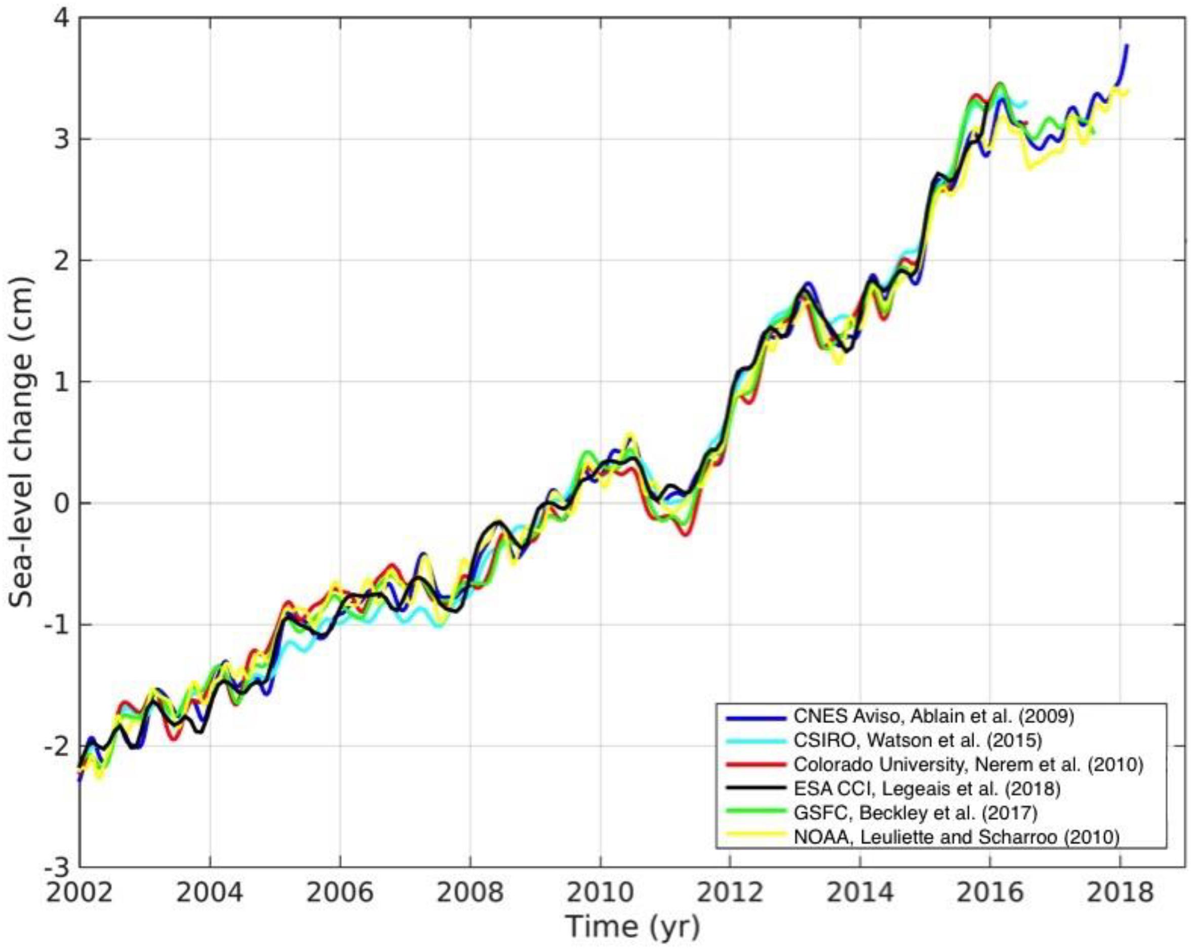
Figure 6. Global mean sea level changes estimated from satellite altimetry by CNES Aviso, CSIRO, Colorado University, Copernicus Climate service, ESA CCI, GSFC, and NOAA.

In the sea level budget approach, the estimate of the OHC trend is derived from the trend in global mean sea level corrected for the mass contribution. The trend in global mean sea level over the last 25 years is of 3.2 mmyr^–1 (e.g., The WCRP Global sea level budget group, 2018) Estimating such a small trend over multi-decadal time scales requires both high accuracy (of a few tenth of mmyr^–1) and high stability in the measurement system over decades. The high stability requirement has been achieved with the series of altimeters T/P, Jason1 Jason 2 and Jason 3 through dedicated inter-calibration phases where a satellite altimeter and it’s successor fly on the same orbit, a few seconds apart. These inter-calibration phases allow for the comparison of precise measurements of the same sea surface topography by different satellite altimeters (Legeais et al., 2018).

Six different groups provide estimates of the trend in global mean sea level (GMSL) from T/P and Jason 1-2-3 (see Figure 6). Over the period 2002–2017 (when GRACE is available to calculate the mass budget) the different groups indicate a sea level rise of 3.3 ± 0.1 mmyr^–1 (1.65 sigma, The WCRP Global sea level budget group, 2018). The spread of ±0.1 mmyr^–1 (1.65 sigma) across these estimates is due to the use of different retracking techniques, different orbit solutions, different corrections and different interpolation methods applied by the different groups (Masters et al., 2012; Henry et al., 2014). This spread is smaller than the uncertainty in the sea level trend because all groups use the same (or similar) methods and corrections to process the altimeter data leading to some potential systematic uncertainty that is not accounted for in the spread.

Two different approaches have been developed to estimate the uncertainty in the trend in sea level so far. The first approach is an error budget approach, which consists of estimating all the possible sources of uncertainty in the satellite measurement system that affect the estimate of the trend in global mean sea level. A careful analysis of all subsystem errors (Ablain et al., 2009, 2015) indicates that the main source of error comes from the correction of the delay in the radar impulse round-trip travel caused by the water content in the atmospheric column (called hereafter the “wet tropospheric correction,” see Table 2). This correction is based on the measurement of a radiometer on board the altimeter that tends to drift with time between two calibrations. This drift causes a spurious drift in the sea level estimate that generates an error of up to ±0.2 mmyr^–1 (5–95% CL) on trends computed over periods less than 10 years (e.g., Legeais et al., 2014; Thao et al., 2014; Fernandes et al., 2015). For decadal and longer trends the error gets smaller because the wet tropospheric signal decorrelates at decadal and longer time scales. The second largest source of error comes from the orbit correction. The errors in the time variable gravity field retrieved with SLR and GRACE and the errors in the realization of the ITRF lead each to an uncertainty of ±0.1 mmyr^–1 in the GMSL trend on annual to multi-decadal time scales (e.g., Couhert et al., 2015). The inter-calibration between satellite altimeters is also a source of uncertainty. The inter-calibration phases allow for the correction of biases between altimeters within an uncertainty of ±0.5 mm for Jason1-2-3 and ±2 mm for T/P in terms of GMSL (Zawadzki and Ablain, 2016; Ablain et al., 2019). This bias uncertainty leads to an uncertainty in the GMSL trend of up to a few tenth of mmyr^–1 for decadal trends (see Figure 7 and Ablain et al., 2019). To a lesser extent the uncertainty in geophysical corrections also lead to some uncertainty in the GMSL trend. In total, the error budget approach indicates an error in the GMSL trend of ±0.5 mmyr^–1 (5–95% CL) on decadal trends, down to ±0.33 mmyr^–1 on 15-year trends (5–95% CL, see Figure 7 and Ablain et al., 2019).

FIGURE 7

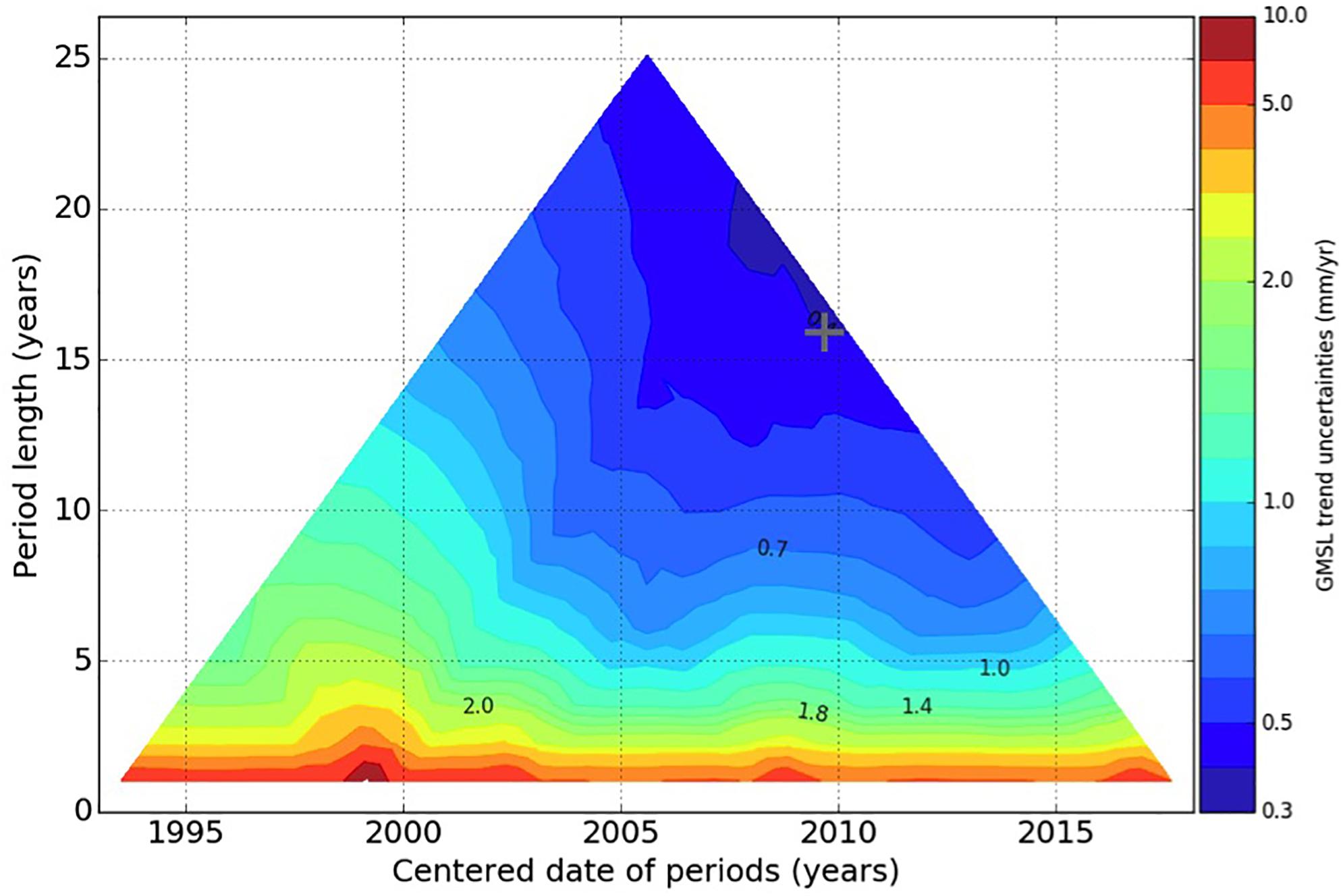
Figure 7. GMSL trend uncertainties (mmyr^–1) estimated for any altimeter period between 1993 and 2017. The Y-axis represents the length of the period over which the trend is computed (in years). The X-axis represents the central date of the period over which the trend is computed (in years). The colorbar indicates the uncertainty associated to trend in sea level. The confidence level is 5–95% (1.65-sigma because we assume a Gaussian distribution). The gray cross indicates the value taken for filling Table 2. Figure updated from Ablain et al. (2019).

The second approach to estimate the error in the GMSL trend is to compare sea level estimates from satellite altimeters with independent estimates from tide gauge records. A careful comparison between altimeters and tide gauges at hundreds of tide gauge sites (Valladeau et al., 2012; Watson et al., 2015) indicates no significant bias between altimeters and tide gauge records at global scale with a RMSE of ±0.4 mmyr^–1 (5–95% CL) over 2002–2017. This uncertainty confirms the results from the error budget approach. Table 2 summarizes the uncertainty estimate over the period of interest here 2002–2017.

There are some limitations in the satellite measurement of sea level. Satellite altimeters do not cover the polar regions (the series T/P and Jason do not reach regions above 66° latitude, the other altimeters reach latitudes up to 82.5° but there are issues in retrieving SSH under sea ice and the sea level estimate in sea ice covered regions is not as accurate). Satellite altimeters do not cover the coastal ocean within 20 km of the coast either (because many geophysical corrections are not valid close to the coast). In addition, satellite altimetry can be affected by systematic drifts that have been accounted for only partially in the error estimate, such as drifts in the ITRF realization or in the glacial isostatic adjustment (GIA) estimate. In the future, progress in interferometry synthetic aperture radar altimetry, which can measure sea level in the leads within sea ice and also close to the coast, should lead to improvements in GMSL trend estimates. Progress in the ITRF realization using assimilation techniques to combine all available geodetic techniques should also lead to improvements (D. Coulot and l’équipe du projet Geodesie, 2017).

For the time-being the only available approach to estimate the error associated with these limitations is to simulate them with models. Several studies (Prandi et al., 2012; Couhert et al., 2015) showed that the associated error on the GMSL trend is likely small (<0.05 mmyr^–1 for the limitation in coverage and <0.06 mmyr^–1 for the limitation due to the ITRF) compared to the total error of ±0.33 mmyr^–1.

Ocean Mass

The ocean mass component of sea level changes is a significant contributor to global mean sea level rise over the last 10–20 years. About 2/3 of the observed sea level change is attributed to mass gain, mostly related to land ice melt on decadal and longer time-scales (The WCRP Global sea level budget group, 2018). On inter-annual timescales, ocean mass changes are modulated by terrestrial water storage changes in response to large-scale precipitation/evaporation variability (i.e., through ENSO). Accurately measuring mass changes on a global scale (both land, ice and oceans) can only be done from space. The GRACE (Gravity Recovery And Climate Experiment) mission, launched in 04/2002 and in operation through 06/2017, provided month-to-month estimates of mass changes, at a spatial resolution of about 300 km (e.g., Wouters et al., 2014). In 05/2018, the GRACE Follow-On mission was launched to continue the GRACE data record.

The measurement system of both missions is similar: two identical satellites orbit the Earth at ∼490 km, and a microwave ranging system tracks minute variations (order if micro-meters) of the separation distance, which is about 220 km. Mass variations at or near the Earth’s surface alter the Earth’s gravity field, which in turn impacts the relative distance between the twin gravimetry satellites. The observations are used to calculate mass changes to an accuracy of ∼1 cm over an area of 300 × 300 km. Averaged over the global oceans, the measurement uncertainty on a monthly time scale is on the order of 1–2 mm. However, as GRACE(-FO) cannot distinguish between the source of the observed gravity change, the isolation of ocean mass from the observations requires several corrections, each of which have different error characteristics. The following corrections are necessary: (1) removing atmospheric mass effects, typically achieved by subtracting the mean atmospheric mass over the oceans from a reanalysis data set (e.g., ERA-Interim), (2) removing long-term trends associated with GIA, typically achieved by subtracting a data-constrained model estimate of the GIA-related gravity signals, and (3) adjusting for signal leakage across the land-ocean boundary due to the limited spatial resolution. While atmospheric mass corrections for ocean mass are considered to be well accounted for, the GIA correction, especially for global ocean mass, is one of the leading error terms. Different GIA corrections can introduce ocean mass trend differences of 0.5 mmyr^–1, mainly due to GIA uncertainty in Antarctica (Blazquez et al., 2018; The WCRP Global sea level budget group, 2018). Signal leakage between the land-ocean boundary, which tends to bias ocean mass changes low, has been addressed in different ways: (1) to obtain unbiased ocean mass directly from conventional GRACE(-FO) observations (so-called spherical harmonic solutions), ocean grid points closer than 300 km from land can be discarded (often referred to as ‘buffer’); (2) so-called mascon solutions (e.g., Watkins et al., 2015) intrinsically address signal leakage via a priori constraints and generally agree with the ‘buffer’ approach; (3) inversion approaches seek to combine GRACE(-FO) observations with other observations (e.g., altimetry, land ice changes, vertical deformation) to obtain an indirect ocean mass estimates (for more details, see for example Wiese et al., 2016b; The WCRP Global sea level budget group, 2018; Uebbing et al., 2019). When compatible correction models (such as GIA) are used, direct and indirect ocean mass estimates agree.

In addition to these corrections, GRACE(-FO) observations need to be augmented with a geocenter offset estimate to take into account center-of-mass to center-of-figure effects on surface mass. Different geocenter estimates exist (using different geodetic data sources and methods), and also contribute to monthly as well as trend uncertainty, on the order of ±0.2 mmyr^–1 (5–95% CL, Blazquez et al., 2018).

The measurement error of GRACE(-FO) is a function of the instrument accuracies, as well as the science data system background models that need to be employed to account for aliasing effects (e.g., tides, sub-monthly ocean and atmosphere changes). Background model uncertainty is somewhat larger than the instrument errors, but on interannual and longer timescales, the corrections from GIA and geocenter trend dominate the error budget (Chen et al., 2013; Blazquez et al., 2018). Over the period 2002–2017 this leads to an uncertainty of ±0.5 mmyr^–1 in the estimation of the ocean mass change (Wiese et al., 2016a).

Sea Level Budget

Following equation (1), the residual of remotely sensed ΔSL_total and ΔSL_mass provides an estimate of ΔSL_thermo. We compare this ΔSL_thermo estimate to estimates derived from in situ measurements (see Figure 2) over the period 2006 to 2015. The in situ measurements of ocean temperature are available for limited ocean depths. With the onset of Argo measurements in 2005, the majority of temperature profiles are available down to ∼ 2000 m depth (see the section “Past and Contemporary Observing Systems for Global OHC”). Technically, the alti-GRACE residual approach provides an independent estimate of ΔSL_thermo representative of the full ocean column and therefore the additional deep ocean contribution (>2000 m) to sea level change that is otherwise estimated by analysis of hydrographic section measurements at about 0.1 ± 0.08 mmyr^–1 (5–95% CL, Purkey and Johnson, 2010; Desbruyères et al., 2016) which correspond to 0.04 ± 0.04 Wm^–2. However, presently the magnitude of measurement uncertainty associated with ΔSL_thermo (±0.5 mmyr^–1, see below) does not allow for the closure of the sea level budget accurately enough to estimate the deep ocean contribution on decadal time scales (The WCRP Global sea level budget group, 2018).

From ΔSL_thermo and with knowledge of the ocean’s expansion efficiency of heat, ε, ΔOHC can be derived (see Equation 2). The period over which we present the published datasets, represents the Argo-era (2006–2015). The global mean ΔSL_total shown in Figure 8 (black line) is a multi-product average based on the six time series presented in section “Sea Level.” The shading indicates the monthly measurement error derived using the error budget approach (see section “Sea Level”) that considers all possible sources of error in the measurement system. We calculate the ΔSL_total trend using weighted least squares regression. The calculated trend is 3.3 ± 0.5 mmyr^–1 (5–95% CL) largely in line with earlier estimates, by Dieng et al. (2017) and The WCRP Global sea level budget group (2018) over similar time period. The time series represent monthly anomalies (mean annual cycle removed) that have been smoothed by applying a 5-month running average filter. The calculation of decadal trend uncertainty is detailed in section “Sea Level.”

FIGURE 8

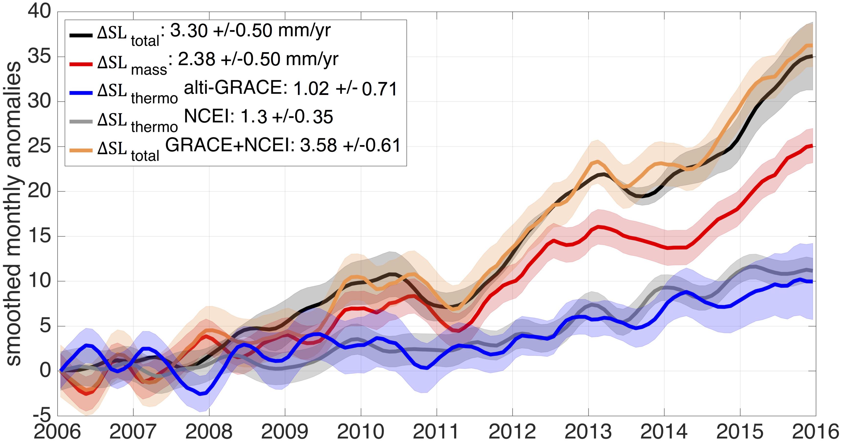
Figure 8. Global mean anomalies of global mean sea level in mm (monthly anomalies, 5-months running means) derived from six altimetry data sets presented in section “Sea Level” (ΔSL_total, black), ocean mass change from four GRACE products (ΔSL_mass, red), thermosteric sea level change as the residual of ΔSL_thermo= ΔSL_total – ΔSL_mass (blue), ΔSL_thermo from NOAA NCEI (gray) based on interpolated seasonal anomalies, and ΔSL_total as the sum of ΔSL_thermo from NCEI and ΔSL_mass (orange). The shadings indicate the measurement uncertainty (5–95% CL); the 5–95% CL trend uncertainties in the legend are provided by the data centers and are detailed in the main text.

ΔSL_mass is a multi-product average (Figure 8, red line) derived from four GRACE-based datasets provided by the Center for Space Research (CSR), the Helmholtz Centre Potsdam, German Research Centre for Geosciences (GFZ), and the Jet Propulsion Laboratory (JPL). The global mean series together with standard errors after Johnson and Chambers (2013) and Chambers et al. (2017) is based on the three institutes’ spherical harmonics products as well as the global mean series from Wiese et al. (2016a) that is based on the JPL mascon product (Watkins et al., 2015). The trend in ΔSL_mass at 2.39 ± 0.5 mmyr^–1 (5–95% CL) is in line with previous estimates from Chambers et al. (2017), Blazquez et al. (2018), and The WCRP Global sea level budget group (2018). The trend uncertainty (5–95% CL) calculation after Wiese et al. (2016a) considers the propagation of monthly uncertainties into the trend, assumes uncorrelated observations, and includes GIA uncertainty according to Chambers et al. (2017). It is important to note that the altimetry and GRACE products do not share the same spatial footprint. This might introduce systematic errors and requires evaluation.

The ΔSL_total −ΔSL_mass residual timeseries is shown in blue on Figure 8 and represents the alti-GRACE time series of ΔSL_thermo. The trend in SL_thermo amounts to 1.02 ± 0.71 mmyr^–1 over 2006–2015 when the mass estimate from GRACE is corrected for the elastic response of the solid Earth (Frederikse et al., 2017; Lickley et al., 2018). The trend uncertainty is calculated assuming the trend uncertainties in ΔSL_total and ΔSL_mass are independent. The in situ estimate of global mean ΔSL_thermo and its standard error (gray) originate from the NOAA National Centers for Environmental Information (NCEI) and represent the thermal expansion of the upper 2000 m ocean column (Levitus et al., 2012). The trend in SL_thermo from NCEI at 1.29 ± 0.35 mmyr^–1 is slightly larger than the SL_thermo trend obtained from the Alti-GRACE residual approach, but in line with estimates over 2005–2016 by von Schuckmann et al. (2018). The associated uncertainty is smaller than the uncertainty in SL_thermo derived from GRACE and altimetry but it is likely biased low as it does not take into account the bias correction errors, the error temporal correlations (see Table 1) and the sampling error.

The orange line represents the ΔSL_total as the sum of in situ ΔSL_thermo and ΔSL_mass and is associated with a trend at 3.58 ± 0.61 mmyr^–1. Accounting for the uncertainties in both ΔSL_total estimates, the sea level budget is considered to be closed. This is in accordance with various studies conducted over the altimetry/GRACE era (e.g., Leuliette and Willis, 2011; Church et al., 2013; Llovel et al., 2014; Feng and Zhong, 2015; Chambers et al., 2017; Dieng et al., 2017). The closure of the sea level budget demonstrate the capability of the sea level budget approach to estimate the ocean thermal expansion. The accuracy of the closure represents the accuracy of the sea level budget approach in estimating the thermal expansion of the ocean. This accuracy is ±0.7 mmyr^–1 (5–95% CL) over 2006–2015. It corresponds to an uncertainty in OHC changes of ±0.37 Wm^–2 (see below).

Estimating the OHC Change From the Ocean Thermal Expansion Change

From the alti-GRACE estimates of ΔSL_thermo, we calculate global mean OHC anomalies by dividing ΔSL_thermo by the expansion efficiency of heat (mYJ^–1) (following Equation 2).

For the expansion efficiency of heat, we adopt here literature values by Kuhlbrodt and Gregory (2012), who estimate ε from in situ observations (Levitus et al., 2012) at 0.12 ± 0.01 mYJ^–1 (equivalent to 0.52 Wm^–2/mmyr^–1) representative of the 0–2000 m ocean column over 1955–2010. Alternate observational estimates by Church et al. (2011) for the full ocean depth over 1972–2008 suggest ε = 0.15 ± 0.03 mYJ^–1, which is not significantly different. The conversion performed is a one-time adjustment, though ε is known to vary spatially and over time and ocean depth. However changes in the global thermal expansion efficiency of heat are likely negligible on decadal time scales because the warming pattern of the ocean is likely the same on decadal time scales (as suggested by climate models, see Kuhlbrodt and Gregory, 2012).

The trend in the OHC series amounts to 0.53 ± 0.38 Wm^–2 over 2006–2015 using ε = 0.12 ± 0.03 mYJ^–1. The associated uncertainty is translated from the trend uncertainty in ΔSL_thermo (±0.37 Wm^–2) and we conservatively add the uncertainty in ε at ±0.03 mYJ^–1 taken from Church et al. (2011) which adds an extra ±0.1 Wm^–2 of uncertainty. The choice of ε plays an important role in modulating the OHC trend estimate from alti-GRACE. Consensus neither exists about the magnitude and uncertainty of ΔSL_thermo from alti-GRACE nor about ε. For example, Fu (2016) found ΔSL_thermo trend at 0.88 mmyr^–1 (2003–2014) that is similar to the estimate presented here, but derived a trend in OHC of 0.66 Wm^–2 using ε = 0.13 mYJ^–1 after Wunsch and Heimbach (2014). Assuming ε = 0.12 ± 0.03 mYJ^–1 yields a change in OHC at 0.52 Wm^–2 per 1 mmyr^–1 change in sea level, which is consistent with Trenberth and Fasullo (2016). Based on this value Dieng et al. (2017) derived an OHC trend from alti-GRACE over 2003–2013 at 0.65 ± 0.1 Wm^–2 (uncertainty represents trend uncertainty only). To avoid systematic errors and to decrease the uncertainty in OHC requires more detailed assessment of ε and ideally the production of ε datasets for the ΔSL_thermo conversion to OHC. These datasets potentially can be derived from observational datasets or ocean reanalysis/models that capture the entire ocean column globally.

Estimating the Global OHC From Ocean Reanalyses

Ocean reanalyses (ORAs) represent an important tool to create a complete picture of ocean variability and climate change based on sparse observations. Typically, ORAs employ an ocean general circulation model (OGCM) and data assimilation schemes to synthesize diverse network of ocean observations ranging from in situ networks to remote sensing systems. An overview of assimilation methods and approaches to ORA is given by Stammer et al. (2016). As summarized there some assimilation approaches are dynamically self-consistent conserving the dynamics embedded into model equations, while other methods violate conservation principles and may be considered as interpolation approaches to ocean observations. Early estimate of the ocean’s role in modulating global energy budget on interannual to decadal timescales (Domingues et al., 2008; Levitus et al., 2009; Ishii and Kimoto, 2009) were only based only on observations and statistical information while during the recent decade more and more products appeared that make use of dynamical information to fill the gaps in the observations.

As part of the international ORA intercomparison project (ORA-IP, Balmaseda et al., 2015), Palmer et al. (2017) used a total of 19 ORAs to intercompare their estimates of various aspects of OHC changes. While the majority of products included a dynamic OGCM, three of the products are still based on statistical analysis of the observations and do not include a dynamic model component. Results indicate that estimates of regional OHC of the top 300 m agree between ORAs over large regions of the Pacific and Indian Oceans over the period 1993–2009. However, at deeper levels, the ORAs are less well-constrained by existing observations leading to substantial differences across the ensemble of existing ORAs, especially in areas of high eddy kinetic energy.

Several studies build on global OHC estimates from ORAs to study the ocean’s role in the Earth’s energy budget and transient climate sensitivity (Balmaseda et al., 2013; Trenberth and Fasullo, 2016; see also von Schuckmann et al., 2018). However, the spread of global OHC estimates of an ensemble of ORAs increase considerably with depth. ORA time series of OHC change in various depth ranges vary in a number of aspects, including: interannual variations; the estimated response to the major volcanic eruptions in 1963, 1982, and 1991 and decadal and multi-decadal trends (Figure 9). The decrease of in situ data coverage available for assimilation is the main factor for large differences at depth layers below 700 m depth (Storto et al., 2015; Palmer et al., 2017). The range of trends and spread among the analyses for the global ocean is similar to the statistical products presented in the Intergovernmental Panel on Climate Change (IPCC) 5th Assessment report (Rhein et al., 2013). A number of products show large initialization or spin-up ‘shock’—i.e., an initial and rapid change in OHC in the first few years of the time series. Separating the time series by hemisphere illustrates the larger spread in the Southern Hemisphere— consistent with the lack of observations over this domain.

FIGURE 9

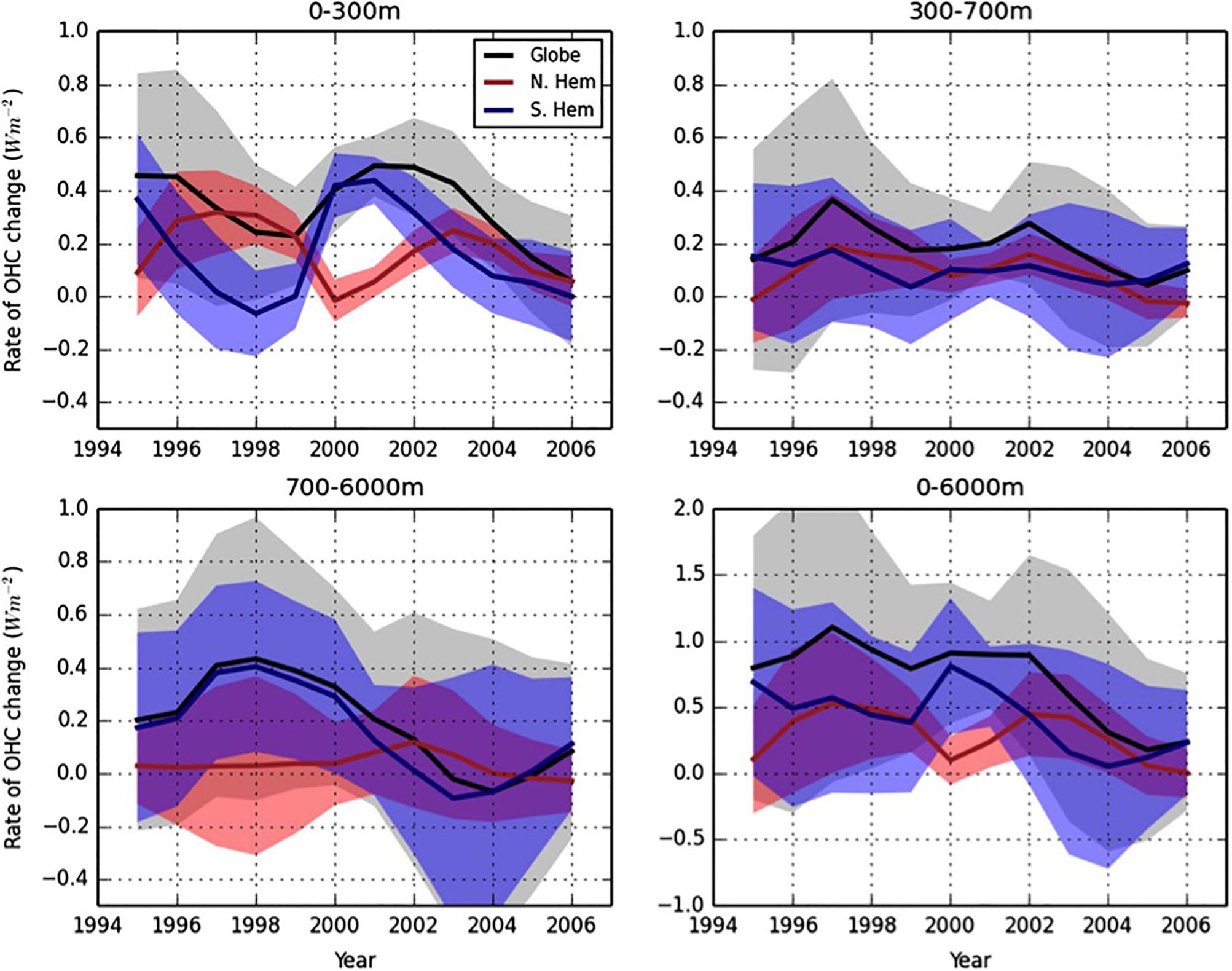
Figure 9. Five-year rolling trends of ocean heat content change over various depth layers for: the Globe (black); Northern Hemisphere (red); and Southern Hemisphere (blue). The solid lines show the ensemble mean with shaded regions indicating ±1 standard deviation. Changes are expressed as equivalent heating rate, in W m^–2, relative to Earth’s surface area. Trends plotted relative to the mid-point of each 5-year period. From Palmer et al. (2017).

Estimated spatial patterns of OHC change for the period 1970–2009 show good agreement in the upper 300 m and are characterized by a strong dipole pattern in the Pacific Ocean (Figure 10). There is less agreement in the patterns of change at deeper levels, potentially linked to differences in the representation of ocean dynamics, such as water mass formation processes. Nevertheless the Atlantic and Southern Oceans are regions in which many ORAs show widespread warming below 700 m over the period 1997–2009.

FIGURE 10

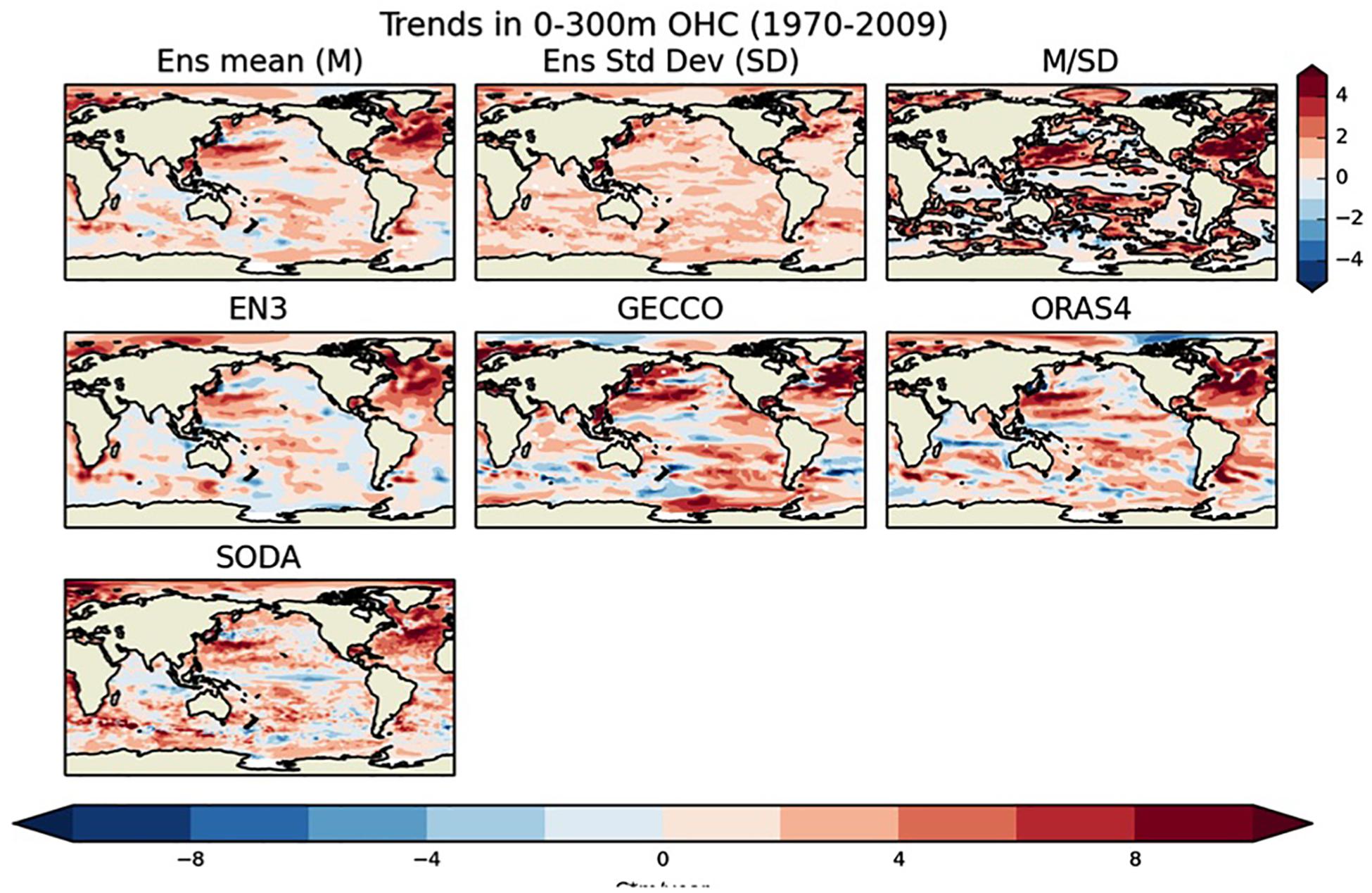
Figure 10. Trends in 0–300 m vertically integrated temperature (Celsius meters per year) for the period 1970–2009. White areas indicate where no data are available. Also shown is the ensemble mean trend (M), the standard deviation of ensemble trends (SD), and the ratio of the two (M/SD). The ensemble values (top row) are computed for each grid box based on all available data (from Palmer et al., 2017).

ORA-based estimates of the past OHC are fundamentally limited by the availability of historical ocean profiles. This holds especially at depths which are considerably under sampled, historically. The intercomparison of ORAs included a reanalysis based on a coupled model (CFSR). In the future more and more of the ORA will be replaced by coupled reanalyses (Penny and Hamill, 2017), in which the combined observations of the atmospheric and ocean compartment can provide a more complete and more consistent picture of the global energy balance of the Earth. Most current ORAs are based on rather coarse resolution models and a further necessary development is the inclusion of the meso-scale in the underlying ocean models due to the importance of upward eddy heat transports for the distribution of heat (Griffies et al., 2015).

Comparison of Global Mean Sea Level Budget, Ocean Heat Content and EEI Estimation

In this section, we compare the OHC estimates obtained from the different approaches described above, namely the remote sensing technique (altimetry and GRACE), the analysis of in situ observations of temperature as well as ocean reanalysis. We furthermore compare time series of Ocean Heat Storage (OHS), the time derivative of OHC, to EEI as measured at TOA from CERES (EBAF, Loeb et al., 2017) dataset. The CERES data is known to be temporally stable (<0.17 Wm^–2 at interannual time scales, Loeb et al., 2018a), but biased in the long-term global mean (and therefore adjusted to agree with long-term OHC trends based on Argo measurements, Loeb et al., 2009). The goal of this comparison is to gain insight into the capabilities and weaknesses of the individual approaches, and to formulate recommendations that lead to improvements in retrieval and the complementary use of the datasets.

Ocean Heat Content

The OHC time series resulting from the sea level budget approach (see Estimating the OHC Change From the Ocean Thermal Expansion Change) is shown in Figure 11 (black line) together with the measurement uncertainty (shading) translated from ΔSL_thermo uncertainty (see Estimating the OHC Change From the Ocean Thermal Expansion Change). For comparison, we show OHC series based on in situ data (OHC_{in situ}) and ocean reanalysis (OHC_rean) in Figure 11. The OHC_{in situ} representative of the 0–2000 m ocean column, is a multi-product time series calculated as the average of four products (PML/JPL/JIMAR, MRI/JMA, NCEI, IAP/CAS) detailed in Johnson et al. (2018) by summing the individual detrended anomalies and trends separately. The series of OHC_{in situ} representative of the 0–700 m column additionally includes series from CSIRO/ACE and the Met Office Hadley Centre. The OHC_rean series for the 0–700 m and 0–2000 m columns are representative of the global oceans between 60°S and 60°N and are based on three reanalysis, GLORYS, C-GLORS, and ORAS5, described in von Schuckmann et al. (2018). Both OHC_{in situ} and OHC_rean are consistent in that they agree on the absolute change in OHC over the period 2006–2015 within given error bars and on the increase in OHC going from the upper 0–700 m to the 0–2000 m column by about 0.3 Wm^–2 (∼40% of 0–2000 m).

FIGURE 11

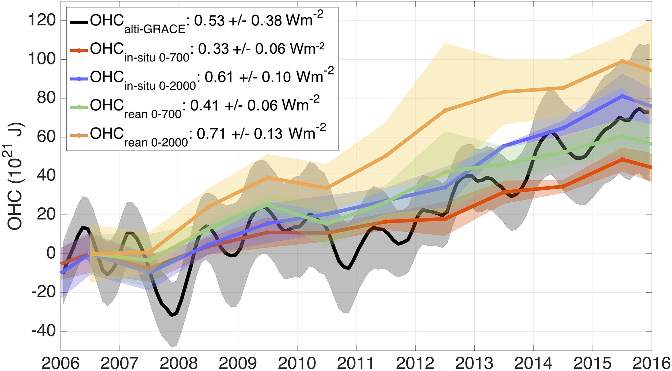
Figure 11. Global mean smoothed (5-month running average) monthly anomalies of OHC derived from alti-GRACE ΔSL_thermo (black, OHC _alti–GRACE), annual mean OHC over the 0–700 m ocean column based on six in situ datasets (OHC_{in situ}, red), annual mean OHC over the 0–2000 m ocean column based on four in situ datasets (OHC_{in situ}, blue), annual mean OHC over the 0–700 m ocean column based on three ocean reanalyses (OHC_rean, green), annual mean OHC over the 0–2000 m ocean column based on three ocean reanalyses (OHC_rean, orange). For OHC_rean and OHC_{in situ}, the shading indicates the spread between timeseries (1.65-sigma). The trend uncertainties represent 5-95% CL from weighted least square regression and adjusted degrees of freedom. For OHC_rean, the trend is adapted from von Schuckmann et al. (2018). The trend 5–95% uncertainty in OHC_alti–GRACE is translated from the trend uncertainty in SLA_thermo and uncertainty in ε (see text in section “Estimating the OHC Change From the Ocean Thermal Expansion Change” and Table 3 for details).

However, overall, the OHC_rean trend at 0.71 Wm^–2 (0–2000 m) is larger by 0.1 Wm^–2 than the OHC_{in situ} trend (0.61 Wm^–2), which is of the order of the trend uncertainty. A slight systematic difference is plausible for different reasons. For example, some of the OHC_{in situ} series are not entirely representative of the global oceans (i.e., PML/JPL/JIMAR) and even if global coverage is provided by including all available ocean profiling data, such as originating from XBT or mooring (see Past and Contemporary Observing Systems for Global OHC), observational sparsity can bias the global reconstructions. OHC_{in situ} based on Argo data only do not fully cover the Arctic and marginal seas. Missing the latter two regions has been shown to reduce the trend in ΔSL_thermo by about 0.25 mmyr^–1 (or 0.13 Wm^–2) as compared to the ocean reanalysis system ORAS4 (Desbruyères et al., 2014; Dieng et al., 2015). On the other hand, OHC_rean exhibits a larger spread especially at deeper levels, linked to differences in the representation of ocean dynamics (Palmer et al., 2017) and the unavailability of in situ data for assimilation (see Estimating the Global OHC From Ocean Reanalyses).

The most recent estimate of EEI at 0.71 ± 0.11 Wm^–2 (OHU over 2006–2015 at 0.68 ± 0.10 Wm^–2 + other forms of heat uptake; Johnson et al., 2016) that is used to constrain space-born radiometric EEI observations (from CERES) is well met by all approaches within their range of uncertainty. In Table 3 we summarize the different OHC trend estimates and find good agreement over 2006–2015 at the 5–95% CL. However some approaches provide more accurate estimates than others. The uncertainty of EEI derived from the Earth surface net heat flux is about 2 orders of magnitude more uncertain than the other estimates hence does not provide any relevant information on the global mean EEI compared to other approaches. The OHC trend based on in situ data is the most accurate of all, with an uncertainty of ±0.11 Wm^–2. This uncertainty may be biased low by as much as ∼0.1 Wm^–2 because it does not take into account the sources of uncertainty due to data distribution (see Table 1 and Lyman and Johnson, 2008). Even after correction of this bias, the in situ approach meets the required accuracy for EEI of ±0.3 Wm^–2 as proposed in the introduction but it does not meet the desired accuracy of ±0.1 Wm^–2. More research is needed to estimate the uncertainty in the in situ estimate of OHC trend, in particular due to data distribution. The ocean reanalyses based estimate of the OHC trend shows a spread of ±0.13 Wm^–2 over 2006–2015 down to 2000 m depth. This spread, which is a lower bound of the uncertainty in the reanalysis estimates, does not decrease the uncertainty compared to the in situ approach. Below 2000 m depth, where very few in situ data are available to constrain the reanalyses, the reanalyses estimates diverge quickly (Palmer et al., 2017) with a spread up to ±0.5 Wm-2 (see Figure 9). Thus, ocean reanalyses does not provide any significant additional constraints on the OHC trend estimates (this is also true for the deep ocean). More research is needed to determine the causes for the spread and the ways of improvement. The remote sensing estimate of OHC trends based on satellite altimetry and GRACE shows an uncertainty of ±0.38 Wm^–2 over 2006–2015 for the global ocean (this estimate includes the uncertainty due to data distribution). This is slightly higher than the required uncertainty of ±0.3 Wm^–2 as proposed in the introduction and further research is needed to improve this uncertainty if this approach is to provide constraints on the EEI estimate. However, it is important to note that a significant part of the uncertainty associated with the remote sensing technique is actually coming from the temporal correlation in errors (in particular in altimetry, see section “Estimating the Ocean Thermal Expansion From Space Observations” and Ablain et al., 2019). This source of uncertainty naturally decays as the period of analysis increases above the error correlation time scales. As a result, the uncertainty in EEI associated with the remote sensing approach is actually expected to reduce below the ±0.3 Wm^–2 limit as the record period becomes longer than ∼15 years. Over the period 2002–2016, the uncertainty associated with the remote sensing approach is already down to ±0.29 Wm^–2 (see Table 3) because of this effect of reduced uncertainty due to temporal correlations in errors.

Interannual Variability in Ocean Heat Uptake and EEI

In the global annual mean, the amplitude and phase in EEI and OHS are expected to be equal, since all other forms of heat uptake are an order of magnitude smaller. Direct measurements of EEI from CERES EBAF are known for their high temporal stability (±0.17 Wm^–2 at interannual time scales, Loeb et al., 2018a), reflecting essentially internal climate variability, such as induced by ENSO (Loeb et al., 2017). In Figure 12, we compare the interannual variability of CERES EBAF EEI with OHS, derived from the temporal gradient in OHC (dOHC/dt), using annual anomalies (long-term mean subtracted) of OHC_rean (0–2000 m) and OHC_{in situ} (0–2000), and annual as well as monthly anomalies (with annual signal removed) for OHC_alti–grace. Pearson correlation coefficients (R) as well as residual root mean square error (RMSE) of the EEI minus each individual OHS time series are provided in Table 3. These measures illustrate the degree of agreement in the phase (R) and in the amplitude (RMSE) of the time series. Although OHS_alti–grace (yellow line) underestimates the amplitude of EEI (red line) (see Figure 12), the series are in phase with a high correlation at R = 0.89, which is in line with the good agreement found by Dieng et al. (2017). Preceding the phase of EEI by 1 year, OHS_rean (blue line) tracks the phase and amplitude of the EEI time series reasonably well (R = 0.50, RMSE = 0.41). For OHS_{in situ} (gray line), both the amplitude and phase are captured well until 2012 (R = 0.85), but including the latter 3 years reduces the R to 0.44. Comparisons with a different subset of OHS_{in situ} by Johnson et al. (2016) yields better correlation at R = 0.78 over 2005–2015. These results strengthen the confidence in the OHS_{in situ}, OHS_alti–grace and CERES measurement systems. When going to shorter time scales and conducting comparisons using monthly anomalies as done with OHS_alti–grace (green line), we expect the agreement to decline. Temporal variability in Argo-derived OHS_{in situ} beyond the decadal and year-to-year scale is overpowered by substantial noise (see Past and Contemporary Observing Systems for Global OHC), owing to measurement errors and spatial coverage deficiencies (e.g., Dieng et al., 2015; Trenberth and Fasullo, 2016). For the monthly anomalies series, the correlation of OHS_alti–grace with CERES EBAF is R = 0.42 and the OHS_alti–grace precedes the phase of CERES by 2 months. While the question of the phase has to be resolved, the significant positive correlation shows some capacity of the Alti-GRACE approach to reproduce the monthly anomalies in EEI. When comparing annual means, as opposed to the monthly anomaly series, all the approaches agree reasonably well in their depiction of interannual variability.

FIGURE 12

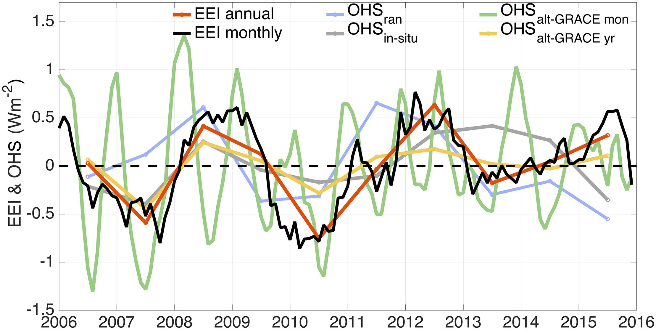
Figure 12. EEI (CERES EBAF) and OHS (dOHC/dt) timeseries from ocean reanalysis (OHS ran), in situ estimation (OHS in situ), and alti-GRACE (OHS alti-GRACE). We show annual timeseries for all parameters (with long-term mean removed) and deseasonalized monthly anomalies for OHS alti-GRACE and EEI that have been smoothed applying a 5-months running average filter.

Conclusion, Synthesis and Perspective

The correlation coefficients and RMSE are provided in Table 3 together with the long-term EEI and OHC trend estimates and their uncertainties derived above. In section “Comparison of Global Mean Sea Level Budget, Ocean Heat Content and EEI Estimation” we paid little attention to the surface net heat flux as a way to approximate global mean EEI, owing to biases and measurement errors two orders of magnitude larger than in the other approaches. In Table 3, we include the global long-term mean (10–15 Wm^–2) and its uncertainty (15 Wm^–2) as presented in section “Estimating the Ocean Surface Net Flux From Space Observations” (e.g., L’Ecuyer et al., 2015). From this comparison it is obvious that a reliable estimate for long-term global mean EEI from surface heat flux is not possible, as there is both substantial overestimation and random error. The limitations of current data products of surface heat flux are outlined in section “Estimating the Ocean Surface Net Flux From Space Observations.” The character of these datasets is complementary to the other approaches, in that they provide constraints at the ocean surface, allow for studies of the separate contributions of ocean and atmospheric energy variability (Liu et al., 2017), and allow regional analysis that can provide information on the magnitude and direction of lateral heat fluxes (e.g., L’Ecuyer et al., 2015). The emerging ITOT method (see Estimating the Ocean Temperature From in situ Observations) is also absent from our comparison because it is an emerging method that is not operational yet and needs further improvements. But we identify it as a promising technique for the future.

The approaches to estimate global mean EEI via the estimation of OHC from either in situ, reanalysis or combined remote sensing techniques, are more reliable and complement each other. The most direct way to estimate OHC is from in situ temperature profiles and represents so far the most accurate method to estimate long-term ocean heat storage. In addition it delivers unprecedented information on how the ocean heat is distributed vertically. Making use of comprehensive ocean models, reanalysis augments the spatial and temporal coverage of OHC physically consistent with dynamical information and provides the means to study sensitivities and uncertainties systemically. But an improvement of OHC trend uncertainty as compared to the in situ approach is not achievable yet. The alti-GRACE sea level budget approach provides a full depth estimate of OHC but is associated with uncertainties that are slightly larger than what is needed to pin down the global mean value of EEI within needed accuracy levels (e.g., Table 3 and von Schuckmann et al., 2016; Hakuba et al., 2018). The alti-Grace approach is promising as it provides consistent spatial and temporal sampling, is representative of the entire global oceans, and estimates OHC over the ocean’s entire depth. A number of issues need to be addressed to improve such datasets, comprising improved estimates of heat expansion efficiencies needed to translate thermosteric sea level change to OHC changes (which relies on in situ measurements of temperature and salinity), analysis of footprint discrepancies and their impact, the retrieval of thermosteric sea level at regional scale including the varying role of halosteric effects, as well as a range of technical challenges in the retrieval of both ΔSL_mass and ΔSL_total, such as inter-calibration, orbit and geocenter corrections, and improved GIA and background models (see Estimating the Ocean Thermal Expansion From Space Observations). To date, only the method employing ocean in situ data (and potentially also the method based on reanalyses, but a robust and comprehensive uncertainty estimate is not yet available) enables to estimate the EEI with the required accuracy of ±0.3 Wm^–2 on decadal time scale. The method based on the altimetry minus GRACE sea level budget reach the same level of accuracy on 15 years time scales. However none of the methods quite reach the desired accuracy of ±0.1 Wm^–2 necessary to analyze hiatus periods or to monitor the EEI response to GHG mitigation policies in the future. Significant improvements in the observing system are necessary in the coming decade if we want to achieve this target. We summarize here the recommendations on the observing system that would enable to reach the accuracy target for EEI estimation.

Recommendation #1 – Sustained observations: The top priority for the observing system from the perspective of EEI estimates is to maintain support for core Argo and to maintain observations of sea level and all contributions to sea level. The sustained observations must be accompanied with research and development activities to improve the climate records (including the record from old satellite missions such as Topex or from old in situ instruments such as XBT) when errors or biases are identified.

Recommendation #2 – Full spatial coverage: Full spatial and temporal implementation of Deep Argo can reduce decadal uncertainties in the deep ocean from ±0.04 to about ±0.006 Wm^–2. A concerted international effort should be made to set up observational campaigns to measure subsurface temperature measurements in areas not presently well covered. These areas include marginal seas, high latitude seasonal ice zones, boundary currents, and shelf regions. Achieving adequate sampling will require an observing system design based on a mixture of observing technologies adopted to the different operating environments. Full spatial coverage including the polar regions of satellite Altimetry will reduce as well the uncertainty in EEI estimate through the alti-grace approach. It is possible to retrieve sea level in the leads over sea ice covered area using new retracking techniques in traditional altimetry (low resolution mode) or using new altimetry techniques like synthetic aperture radar altimetry. The objective is to provide sea level estimates up to 82°N over the last 2 decades with old missions (like ERS 1 and 2 and ENVISAT) and to provide sea level estimates up to 88°N over the last 7 years with recent polar missions such as CRYOSAT.

Recommendation #3 – Uncertainties: Over the last decade progress has been made in quantifying uncertainties in estimates of in situ temperatures, sea level, ocean mass and its contributors. But it is still necessary to improve the uncertainty estimates. Uncertainties should be validated against other independent observations when possible. This is essential to increase the confidence in the EEI estimate. There are several directions of improvements:

(1) The first direction is to improve the uncertainty in in situ temperature. This is possible by developing/maintaining multiple platform observations for cross-validation and calibration purposes for current Argo measurements in the upper 2000m depth, as well as for new extensions such as deep Argo.

(2) The second direction is to get a better confidence in GRACE uncertainty of ocean mass estimates by validation against independent data sources. Independent estimates of the ocean mass can be obtained through the ocean freshwater budget (Munk, 2003). This implies to improve the salinity record from Argo and the sea ice thickness estimate from altimetry.

(3) The third direction is to improve altimetry uncertainty by reducing the uncertainty in orbit determination (which depends on the accuracy of the gravity field prior of GRACE and the accuracy of the geocenter motion estimate) and by revisiting the uncertainty in the wet tropospheric correction (which can show biases with respect to independent estimates from SSMI satellites). To get higher confidence in altimetry uncertainty the comparison with tide gauge records should also be improved. This is possible by equipping more tide gauge records with global positioning system in order to improve tide gauge measurement of the absolute sea level and improve the comparison with satellite altimetry at both global and regional scale.

Author Contributions

This manuscript resulted from the merger, suggested by OceanObs’19 organizers, of three different abstracts led by BM, TB, and ZZ. BM, TB, and ZZ led and designed the manuscript. All authors participated in the discussions and writing that led to the final contents of the manuscript.

Funding

GJ was supported by the NOAA Research. MP and RK were supported by the Met Office Hadley Centre Climate Programme funded by BEIS and Defra. JC was partially supported by the Centre for Southern Hemisphere Oceans Research, a joint research centre between QNLM and CSIRO. CD and AS were funded by the Australian Research Council (FT130101532 and DP160103130) and its Centre of Excellence for Climate Extremes (CLEX). IQuOD team members (TB, RC, LC, CD, VG, MI, MP, and SW) were supported by the Scientific Committee on Oceanic Research (SCOR) Working Group 148, funded by the National SCOR Committees and a grant to SCOR from the U.S. National Science Foundation (Grant OCE-1546580), as well as the Intergovernmental Oceanographic Commission of UNESCO/International Oceanographic Data and Information Exchange (IOC/IODE) IQuOD Steering Group. ZZ was supported by the National Aeronautics and Space Administration (NNX17AH14G). LC was supported by the National Key Research and Development Program of China (2017YFA0603200 and 2016YFC1401800).

Conflict of Interest Statement

The authors declare that the research was conducted in the absence of any commercial or financial relationships that could be construed as a potential conflict of interest.

Acknowledgments

We thank the CNES AVISO project and the ESA CCI project for making their sea level data freely available. PMEL Contribution Number 4865.

Footnotes

1. ^ http://www.goosocean.org
2. ^ www.iquod.org
3. ^ http://sio-argo.ucsd.edu/RG_Climatology.html

References

Ablain, M., Cazenave, A., Larnicol, G., Balmaseda, M., Cipollini, P., Faugère, Y., et al. (2015). Improved sea level record over the Satellite Altimetry Era (1993–2010) from the climate change initiative project. Ocean Sci. 11, 67–82. doi: 10.5194/os-11-67-2015

CrossRef Full Text | Google Scholar

Ablain, M., Cazenave, A., Valladeau, G., and Guinehut, S. (2009). A new assessment of the error budget of global mean sea level rate estimated by satellite altimetry over 1993–2008. Ocean Sci. 5, 193–201. doi: 10.5194/os-5-193-2009

CrossRef Full Text | Google Scholar

Ablain, M., Meyssignac, B., Zawadzki, L., Jugier, R., Ribes, A., Cazenave, A., et al. (2019). Uncertainty in satellite estimate of global mean sea level changes, trend and acceleration. Earth Syst. Sci. Data Discuss. 1–26. doi: 10.5194/essd-2019-10

CrossRef Full Text | Google Scholar

Abraham, J. P., Baringer, M., Bindoff, N. L., Boyer, T., Cheng, L. J., Church, J. A., et al. (2013). A review of global ocean temperature observations: implications for ocean heat content estimates and climate change. Rev. Geophys. 51, 450–483. doi: 10.1002/rog.20022

CrossRef Full Text | Google Scholar

Allan, R. P., Liu, C., Loeb, N. G., Palmer, M. D., Roberts, M., Smith, D., et al. (2014). Changes in global net radiative imbalance 1985–2012. Geophys. Res. Lett. 41, 5588–5597. doi: 10.1002/2014GL060962

PubMed Abstract | CrossRef Full Text | Google Scholar

Andreas, E. L. (1992). Sea spray and the surbulent air-sea heat fluxes. J. Geophys. Res. 97, 11429–11441. doi: 10.1029/92jc00876

CrossRef Full Text | Google Scholar

Argo Science Team (1999). Report of the Argo Science Team Meeting (Argo-1). Melbourne: GODAE International Project Office, 27.

Google Scholar

Balmaseda, M. A., Hernandez, F., Storto, A., Palmer, M. D., Alves, O., Shi, L., et al. (2015). The ocean reanalyses intercomparison project (ORA-IP). J. Operat. Oceanogr. 8, (Suppl. 1), s80–s97. doi: 10.1080/1755876X.2015.1022329

CrossRef Full Text | Google Scholar

Balmaseda, M. A., Trenberth, K. E., and Källén, E. (2013). Distinctive climate signals in reanalysis of global ocean heat content. Geophys. Res. Lett. 40, 1754–1759. doi: 10.1002/grl.50382

CrossRef Full Text | Google Scholar

Beckley, B. D., Callahan, P. S., Hancock, D. W., Mitchum, G. T., and Ray, R. D. (2017). On the ‘Cal-Mode’ correction to TOPEX satellite altimetry and its effect on the global mean sea level time series. J. Geophys. Res. Oceans 122, 8371–8384. doi: 10.1002/2017jc013090

CrossRef Full Text | Google Scholar

Beckley, B. D., Lemoine, F. G., Luthcke, S. B., Ray, R. D., and Zelensky, N. P. (2007). A reassessment of global and regional mean sea level trends from TOPEX and Jason-1 altimetry based on revised reference frame and orbits. Geophys. Res. Lett. 34:L14608. doi: 10.1029/2007GL030002

CrossRef Full Text | Google Scholar

Benveniste, J. (2011). “Radar altimetry: past, present and future,” in Coastal Altimetry, eds S. Vignudelli, A. Kostianoy, P. Cipollini, and J. Benveniste (Berlin: Springer), 1–17. doi: 10.1007/978-3-642-12796-0_1

CrossRef Full Text | Google Scholar

Bindoff, N. L., Stott, P. A., AchutaRao, K. M., Allen, M. R., Gillett, N., Gutzler, D., et al. (2013). “Detection and attribution of climate change: from global to regional,” in Climate Change 2013: The Physical Science Basis. Contribution of Working Group I to the Fifth Assessment Report of the Intergovernmental Panel on Climate Change, eds T. F. Stocker, D. Qin, G.-K. Plattner, M. Tignor, S. K. Allen, J. Boschung, et al. (Cambridg: Cambridge University Press).

Google Scholar

Blazquez, A., Meyssignac, B., Lemoine, J. M., Berthier, E., Ribes, A., and Cazenave, A. (2018). Exploring the uncertainty in GRACE estimates of the mass redistributions at the Earth surface: implications for the global water and sea level budgets. Geophys. J. Int. 215, 415–430. doi: 10.1093/gji/ggy293

CrossRef Full Text | Google Scholar

Boyer, T., Domingues, C. M., Good, S. A., Johnson, G. C., Lyman, J. M., Ishii, M., et al. (2016). Sensitivity of global upper ocean heat content estimates to mapping methods, XBT bias corrections, and baseline climatologies. J. Clim. 29, 4817–4842. doi: 10.1175/JCLI-D-15-0801.1

CrossRef Full Text | Google Scholar

Boyer, T. P., Antonov, J. I., Baranova, O. K., Coleman, C., Garcia, H. E., Grodsky, A., et al. (2013). World Ocean Database 2013. Silver Spring, MD: NOAA Printing Officce, 208.

Google Scholar

Chambers, D. P., Cazenave, A., Champollion, N., Dieng, H., Llovel, W., Forsberg, R., et al. (2017). Evaluation of the global mean sea level budget between 1993 and 2014. Surv. Geophys. 38:309. doi: 10.1007/s10712-016-9381-3

CrossRef Full Text | Google Scholar

Chelton, D. B., Ries, J. C., Haines, B. J., Fu, L.-L., and Callahan, P. S. (2001). “Satellite altimetry,” in Satellite Altimetry and Earth Sciences, Vol. 69, eds L. Fu and A. Cazenave (New York, NY: Elsevier), 1–131.

Google Scholar

Chen, J. L., Wilson, C. R., and Tapley, B. D. (2013). Contribution of ice sheet and mountain glacier melt to recent sea level rise. Nat. Geosci. 9, 549–552. doi: 10.1038/NGEO1829

CrossRef Full Text | Google Scholar

Cheng, L., Abraham, J., Goni, G., Boyer, T., Wijffels, S., Cowley, R., et al. (2016a). XBT science: assessment of instrumental biases and errors. Bull. Am. Meterol. Soc. 96, 924–933. doi: 10.1175/BAMS-D-15-00031.1

CrossRef Full Text | Google Scholar

Cheng, L., Abraham, J., Hausfather, Z., and Trenberth, K. E. (2019). How fast are the oceans warming? Science 363, 128–129. doi: 10.1126/science.aav7619

PubMed Abstract | CrossRef Full Text | Google Scholar

Cheng, L., Luo, H., Boyer, T., Cowley, R., Abraham, J., Gouretski, V., et al. (2018). How well can we correct systematic errors in historical XBT data? J. Atmos. Oceanic Technol. 35, 1103–1125. doi: 10.1175/JTECH-D-17-0122.1

CrossRef Full Text | Google Scholar

Cheng, L., Trenberth, K. E., Boyer, T., Fasullo, J., Zhu, L., and Abraham, J. (2017). Improved estimates of ocean heat content from 1960-2015. Sci. Adv. 3:e1601545. doi: 10.1126/sciadv.1601545

PubMed Abstract | CrossRef Full Text | Google Scholar

Cheng, L., Trenberth, K. E., Palmer, M. D., Zhu, J., and Abraham, J. P. (2016b). Observed and simulated full-depth ocean heat-content changes for 1970–2005. Ocean Sci. 12, 925–935. doi: 10.5194/os-12-925-2016

CrossRef Full Text | Google Scholar

Cheng, L., and Zhu, J. (2014a). Artifact in variations of ocean heat content induced by the observation system changes. Geophys. Res. Lett. 41, 7276–7283. doi: 10.1002/2014GL061881

CrossRef Full Text | Google Scholar

Cheng, L., and Zhu, J. (2014b). Uncertainties of the ocean heat content estimation induced by insufficient vertical resolution of historical ocean subsurface observations. J. Atmos. Oceanic Technol. 31, 1383–1396. doi: 10.1175/JTECH-D-13-00220.1

CrossRef Full Text | Google Scholar

Cheng, L., and Zhu, J. (2015). Influences of the choice of climatology on ocean heat content estimation. J. Atmos. Oceanic Technol. 32, 388–394. doi: 10.1175/JTECH-D-14-00169.1

CrossRef Full Text | Google Scholar

Cheng, L., Zhu, J., Cowley, R., Boyer, T., and Wijffels, S. (2014). Time, probe type and temperature variable bias corrections to historical expendable bathythermograph observations. J. Atmos. Oceanic Technol. 31, 1793–1825. doi: 10.1175/JTECH-D-13-00197.1

CrossRef Full Text | Google Scholar

Church, J. A., Clark, P. U., Cazenave, A., Gregory, J. M., Jevrejeva, S., Levermann, A., et al. (2013). “Sea level change,” in Climate Change 2013: The Physical Science Basis. Contribution of Working Group I to the Fifth Assessment Report of the Intergovernmental Panel on Climate Change, eds T. F. Stocker, D. Qin, G.-K. Plattner, M. Tignor, S. K. Allen, J. Boschung, et al. (Cambridge: Cambridge University Press), 1137–1216.

Google Scholar

Church, J. A., White, N. J., Konikow, L. F., Domingues, C. M., Graham Cogley, J., Rignot, E., et al. (2011). Revisiting the Earth’s sea-level and energy budget from 1961 to 2008. Geophys. Res. Lett. 38:L18601. doi: 10.1029/2011GL048794

CrossRef Full Text | Google Scholar

Collins, W. D., Rasch, P. J., Eaton, B. E., Khattatov, B. V., Lamarque, J.-F., and Zender, C. S. (2001). Simulating aerosols using a chemical transport model with assimilation of satellite aerosol retrievals: methodology for INDOEX. J. Geophys. Res. 106, 7313–7336. doi: 10.1029/2000JD900507

CrossRef Full Text | Google Scholar

Couhert, A., Cerri, L., Legeais, J. F., Ablain, M., Zelensky, N. P., Haines, B. J., et al. (2015). Towards the 1mm/y stability of the radial orbit error at regional scales. Adv. Space Res. 55, 2–23. doi: 10.1016/j.asr.2014.06.041

CrossRef Full Text | Google Scholar

Cowley, R., Wijffels, S., Cheng, L., Boyer, T., and Kizu, S. (2013). Biases in expendable bathythermograph data: a new view based on historical side-by-side comparisons. J. Atmos. Ocean. Technol. 30, 1195–1225. doi: 10.1175/JTECH-D-12-00127.1

CrossRef Full Text | Google Scholar

Cox, C., and Munk, W. (1954). Measurement of the roughness of the sea surface from photographs of the Sun’s glitter. J. Opt. Soc. Am. 44, 838–850.

Google Scholar

Cronin, M. F., Weller, R. A., Lampitt, R. S., and Send, U. (2012). “Ocean reference stations,” in Earth Observation, eds R. B. Rustamov and S. E. Salahova (London: IntechOpen). Available at: https://www.intechopen.com/books/earth-observation/ocean-reference-stations

Google Scholar

D. Coulot and l’équipe du projet Geodesie (2017). “Assimilation de données géodésiques et estimation de références pour l’étude du changement climatique,” in Paper Présented at the Projet of ANR GEODESIE. XYZ, (Saint-Mandé: Association française de topographie (AFT)), 39–46.

Google Scholar

Davies, J. H., and Davies, D. R. (2010). Earth’s surface heat flux. Solid Earth 1, 5–24. doi: 10.5194/se-1-5-2010

PubMed Abstract | CrossRef Full Text | Google Scholar

Desbruyères, D. G., McDonagh, E. L., King, B. A., Garry, F. K., Blaker, A. T., and Moat, B. I, et al. (2014). Full-depth temperature trends in the northeastern Atlantic through the early 21st century. Geophys. Res. Lett. 41, 7971–7979. doi: 10.1002/(ISSN)1944-8007

CrossRef Full Text | Google Scholar

Desbruyères, D. G., Purkey, S. G., McDonagh, E. L., Johnson, G. C., and King, B. A. (2016). Deep and abyssal ocean warming from 35 years of repeat hydrography. Geophys. Res. Lett. 43, 356–310. doi: 10.1002/2016GL070413

CrossRef Full Text | Google Scholar

Dieng, H. B., Cazenave, A., Meyssignac, B., von Schuckmann, K., and Palanisamy, H. (2017). Sea and land surface temperatures, ocean heat content, Earth’s energy imbalance and net radiative forcing over the recent years. Int. J. Climatol. 37, 218–229. doi: 10.1002/joc.4996

PubMed Abstract | CrossRef Full Text | Google Scholar

Dieng, H. B., Cazenave, A., von Schuckmann, K., Ablain, M., and Meyssignac, B. (2015). Sea level budget over(2005)–2013: missing contributions and data errors. Ocean Sci. 11, 789–802. doi: 10.5194/os-11-789-2015

CrossRef Full Text | Google Scholar

Domingues, C., and Palmer, M. (2015). The IQuOD initiative: towards an international quality controlled ocean database. CLIVAR Exchanges 67, 38–40.

Google Scholar

Domingues, C. M., Church, J. A., White, N. J., Gleckler, P. J., Wijffels, S. E., Barker, P. M., et al. (2008). Improved estimates of upper-ocean warming and multi-decadal sea-level rise. Nature 453, 1090–1093. doi: 10.1038/nature07080

PubMed Abstract | CrossRef Full Text | Google Scholar

Dong, X., Xu, K., Liu, H., and Jiang, J. (2004). “The radar altimeter and scatterometer of China’s HY-2 satellite,” in Proceedings of the IEEE International Geoscience and Remote Sensing Symposium 2004, Vol. 13, (Anchorage, AK), 1703–1706. doi: 10.1109/IGARSS.2004.1370659

CrossRef Full Text | Google Scholar

Durack, P. J., Gleckler, P. J., Landerer, F. W., and Taylor, K. E. (2014). Quantifying underestimates of long-term upper-ocean warming. Nat. Clim. Change 4, 999–1005. doi: 10.1038/nclimate2389

CrossRef Full Text | Google Scholar

Dushaw, B., Au, W., Beszczynska-Moller, A., Brainard, D., Bruce, D. C., Duda, T., et al. (2009). “A Global Ocean Acoustic Observing Network,” in Proceedings of OceanObs’09: Sustained Ocean Observations and Information for Society, Vol. 2. Venice: European Space Agency, 279–291. doi: 10.5270/OceanObs09.cwp.25

CrossRef Full Text | Google Scholar

Dushaw, B. D. (2018). Ocean acoustic tomography in the North Atlantic. J. Atmos. Oceanic Technol. 36, 183–202. doi: 10.1175/JTECH-D-18-0082.1

CrossRef Full Text | Google Scholar

Ellingson, R. G. (1995). Surface longwave fluxes from satellite observations: a critical review. Remote Sens. Environ. 51, 89–97. doi: 10.1016/0034-4257(94)00067-W

CrossRef Full Text | Google Scholar

Eriksen, C. C. (2017). Deep gliders for observing circulation and climate. US CLIVAR Variat. 2, 34–38.

Google Scholar

Fairall, C. W., Bradley, E. F., Hare, J. E., Grachev, A. A., and Bdson, J. B. (2003). Bulk parameterization of air-sea fluxes: update and verification for the COARE algorithm. J. Clim. 16, 571–591. doi: 10.1175/1520-0442(2003)016<0571:bpoasf>2.0.co;2

CrossRef Full Text | Google Scholar

Fairall, C. W., Bradley, E. F., Rogers, D. P., Edson, J. B., and Young, G. S. (1996). Bulk parameterization of air-sea flux for tropical ocean-global atmosphere coupled-ocean atmosphere response experiment. J. Geophys. Res. 101, 3747–3746.

Google Scholar

Fasullo, J. T., and Trenberth, K. E. (2008). The annual cycle of the energy budget Part I: global mean and land-ocean exchange. J. Clim. 21, 2297–2312. doi: 10.1175/2007JCLI11935.1

CrossRef Full Text | Google Scholar

Feng, W., and Zhong, M. (2015). Global sea level variations from altimetry, GRACE and Argo data over 2005–2014. Geod. Geodyn. 6:4. doi: 10.1016/j.geog.2015.07.001

CrossRef Full Text | Google Scholar

Fernandes, M. J., Lázaro, C., Ablain, M., and Pires, N. (2015). Improved wet path delays for all ESA and reference altimetric missions. Remote Sens. Environ. 169, 50–74. doi: 10.1016/j.rse.2015.07.023

CrossRef Full Text | Google Scholar

Forsyth, J. S. T., Andres, M., and Gawarkiewicz, G. G. (2015). Recent accelerated warming of the continental shelf off New Jersey: observations from the CMV Oleander expendable bathythermograph line. J. Geophys. Res. Oceans 120, 2370–2384. doi: 10.1002/2014JC010516

CrossRef Full Text | Google Scholar

Foster, G., and Rahmstorf, S. (2011). Global temperature evolution 1979–2010. Environ. Res. Lett. 6:044022. doi: 10.1088/1748-9326/6/4/044022

CrossRef Full Text | Google Scholar

Frederikse, T., Riva, R. E. M., and King, M. A. (2017). Ocean bottom deformation due to present-day mass redistribution and its impact on sea level observations. Geophys. Res. Lett. 44, 306–312. doi: 10.1002/2017GL075419

CrossRef Full Text | Google Scholar

Fu, L.-L. (2016). On the decadal trend of global mean sea level and its implication on ocean heat content change. Front. Mar. Sci. 3:37. doi: 10.3389/fmars.2016.00037

CrossRef Full Text | Google Scholar

Good, S. A., Martin, M. J., and Rayner, N. A. (2013). EN4: quality controlled ocean temperature and salinity profiles and monthly objective analyses with uncertainty estimates. J. Geophys. Res. Oceans 118, 6704–6716. doi: 10.1002/2013JC009067

CrossRef Full Text | Google Scholar

Gouretski, V. (2012). Using GEBCO digital bathymetry to infer depth biases in the XBT data. Deep-Sea Res. I 62, 40–52. doi: 10.1016/j.dsr.2011.12.012

CrossRef Full Text | Google Scholar

Gouretski, V. (2018). World ocean circulation experiment – argo global hydrographic climatology. Ocean Sci. 14, 1127–1146. doi: 10.5194/os-14-1127-2018

CrossRef Full Text | Google Scholar

Gouretski, V., Jungclaus, J., and Haack, H. (2013). Revisiting the Meteor 1925–1927 hydrographic dataset reveals centennial full-depth changes in the Atlantic Ocean. Geophys. Res. Lett. 40, 2236–2224. doi: 10.1002/grl.50503

CrossRef Full Text | Google Scholar

Gouretski, V., and Koltermann, K. P. (2007). How much is the ocean really warming? Geophys. Res. Lett. 34:L01610. doi: 10.1029/2006GL027834

CrossRef Full Text | Google Scholar

Gouretski, V., and Reseghetti, V. (2010). On depth and temperature biases in bathythermograph data: development of a new correction scheme based on analysis of a global ocean database. Deep Sea Res. Part I Oceanogr. Res. Pap. 57, 812–833. doi: 10.1016/j.dsr.2010.03.011

CrossRef Full Text | Google Scholar

Gregory, J. M., Griffies, S. M., Hughes, C. W., Lowe, J. A., Church, J. A., Fukimori, I., et al. (2019). Concepts and terminology for sea level: mean, variability and change, both local and global. Surv. Geophys. 1–39. doi: 10.1007/s10712-019-09525-z

CrossRef Full Text | Google Scholar

Griffies, S. M., Winton, M., Anderson, W. G., Benson, R., Delworth, T. L., Dufour, C. O., et al. (2015). Impacts on ocean heat from transient mesoscale eddies in a hierarchy of climate models. J. Clim. 28, 952–977. doi: 10.1175/jcli-d-14-00353.1

CrossRef Full Text | Google Scholar

Hakuba, M. Z., Stephens, G. L., Bruno, C., Nash, A. N., Foulon, B., Bettadpur, S. V., et al. (2018). Earth’s energy imbalance measured from space. IEEE Trans. Geosci. Remote Sens. 57, 32–45. doi: 10.1109/TGRS.2018.2851976

CrossRef Full Text | Google Scholar

Hansen, J., Sato, M., Kharecha, P., and von Schuckmann, K. (2011). Earth’s energy imbalance and implications. Atmos. Chem. Phys. 11, 13421–13449. doi: 10.5194/acp-11-13421-2011

CrossRef Full Text | Google Scholar

Hartmann, D. L., Klein Tank, A. M. G., Rusticucci, M., Alexander, L. V., Brönnimann, S., Rahman Charabi, Y. A., et al. (2013). “Observations: atmosphere and surface, climate change 2013: the physical science basis,” in Proceedings of the Working Group I Contribution to the Fifth Assessment Report of the Intergovernmental Panel on Climate Change, (Cambridge: Cambridge University Press), 159–254. doi: 10.1017/cbo9781107415324.008

CrossRef Full Text | Google Scholar

Hedemann, C., Mauritsen, T., Jungclaus, J., and Marotzke, J. (2017). The subtle origins of surface-warming hiatuses. Nat. Clim. Change 7, 336–339. doi: 10.1038/nclimate3274

CrossRef Full Text | Google Scholar

Henry, O., Ablain, M., Meyssignac, B., Cazenave, A., Masters, D., Nerem, S., et al. (2014). Investigating and reducing differences between the satellite altimetry-based global mean sea level time series provided by different processing groups. J. Geod. 88, 351–361. doi: 10.1007/s00190-013-0687-3

CrossRef Full Text | Google Scholar

Howe, B., Worcester, P., Sagen, H., et al. (2019). The roles of underwater acoustics in observing the global ocean. Front. Mar. Sci.

Google Scholar

IOC, SCOR, and IAPSO (2010). The International Thermodynamic Equation of Seawater – 2010: Calculation and Use of Thermodynamic Properties. Intergovernmental Oceanographic Commission, Manuals and Guides No. 56. Paris: UNESCO, 196.

Google Scholar

Ishii, M., Fakuda, Y., Hirahara, S., Yasui, S., Suzuki, T., and Sato, K. (2017). Accuracy of global upper ocean heat content estimation expected from present observational data sets. SOLA 13, 163–167. doi: 10.2151/sola.2017-030

CrossRef Full Text | Google Scholar

Ishii, M., and Kimoto, M. (2009). Reevaluation of historical ocean heat content variations with time-varying XBT and MBT depth bias corrections. J. Oceanogr. 65, 287–299. doi: 10.1007/s10872-009-0027-7

CrossRef Full Text | Google Scholar

Jayne, S. R., Roemmich, D., Zilberman, N., Riser, S. C., Johnson, K. S., Johnson, G. C., et al. (2017). The argo program present and future. Oceanography. 30, 18–28. doi: 10.5670/oceanog.2017.213

CrossRef Full Text | Google Scholar

Jin, Z., Charlock, T. P., Smith, W. L. Jr., and Rutledge, K. (2004). A parameterization ocean surface albedo. Geophys. Res. Lett. 31:L22301. doi: 10.1029/2004GL021180

CrossRef Full Text | Google Scholar

Johnson, G. C., and Birnbaum, A. N. (2017). As El Nino builds, Pacific Warm Pool expands, ocean gains more heat. Geophys. Res. Lett. 44, 438–445. doi: 10.1002/2016gl071767

CrossRef Full Text | Google Scholar

Johnson, G. C., and Chambers, D. (2013). Ocean bottom pressure seasonal cycles and decadal trends from GRACE Release-05: ocean circulation implications. J. Geophys. Res. Oceans 118, 4228–4240. doi: 10.1002/jgrc.20307

CrossRef Full Text | Google Scholar

Johnson, G. C., Lyman, J. M., Boyer, T., Cheng, L., Domingues, C. M., Gilson, J., et al. (2018). Ocean heat content. In State of the Climate in 2017. Bull. Am. Meteorol. Soc. 99, S72–S77. doi: 10.1175/2018BAMSStateoftheClimate.1

CrossRef Full Text | Google Scholar

Johnson, G. C., Lyman, J. M., and Loeb, N. G. (2016). CORRESPONDENCE: improving estimates of Earth’s energy imbalance. Nat. Clim. Change 6, 639–640. doi: 10.1038/nclimate3043

CrossRef Full Text | Google Scholar

Johnson, G. C., Lyman, J. M., and Purkey, S. G. (2015). Informing deep argo array design using argo and full- depth hydrographic section data. J. Atmos. Oceanic Technol. 32, 2187–2198. doi: 10.1175/JTECH-D-15-0139.1

CrossRef Full Text | Google Scholar

Kato, S., Rose, F. G., Rutan, D. A., Thorsen, T. J., Loeb, N. G., Doelling, D. R., et al. (2018). Surface irradiances of edition 4.0 clouds and the earth’s radiant energy system (CERES) energy balanced and filled (EBAF) data product. J. Clim. 31, 4501–4527. doi: 10.1175/JCLI-D-17-0523.1

CrossRef Full Text | Google Scholar

Kato, S., Rose, F. G., Sun-Mack, S., Miller, W. F., Chen, Y. R., David, A. S., et al. (2011). Improvements of top-of-atmosphere and surface irradiance computations with CALIPSO-, CloudSat-, and MODIS-derived cloud and aerosol properties. J. Geophys. Res. 116:D19209. doi: 10.1029/2011JD016050

CrossRef Full Text | Google Scholar

Kato, S., Xu, K.-M., Wong, T., Loeb, N. G., Rose, F. G., Trenberth, K. E., et al. (2016). Investigation of the bias in column integrated atmospheric energy balance using cloud objects. J. Clim. 29, 7435–7452. doi: 10.1175/JCLI-D-15-0782.1

CrossRef Full Text | Google Scholar

Kuhlbrodt, T., and Gregory, J. M. (2012). Ocean heat uptake and its consequences for the magnitude of sea level rise and climate change. Geophys. Res. Lett. 39:L18608. doi: 10.1029/2012GL052952

CrossRef Full Text | Google Scholar

Kuusela, M., and Stein, M. L. (2018). Locally stationary spatio-temporal interpolation of Argo profiling float data. Proc. R. Soc. A 474:20180400. doi: 10.1098/rspa.2018.0400

PubMed Abstract | CrossRef Full Text | Google Scholar

L’Ecuyer, T., Beaudoing, H. K., Rodell, M., Olson, W., Lin, B., and Kato, S. (2015). The observed state of the energy budget in the early 21st century. J Clim. 28, 8319–8346. doi: 10.1175/JCLI-D-14-00556.1

CrossRef Full Text | Google Scholar

Legeais, J.-F., Ablain, M., and Thao, S. (2014). Evaluation of wet troposphere path delays from atmospheric reanalyses and radiometers and their impact on the altimeter sea level. Ocean Sci. 10, 893–905. doi: 10.5194/os-10-893-2014

CrossRef Full Text | Google Scholar

Legeais, J.-F., Ablain, M., Zawadzki, L., Zuo, H., Johannessen, J. A., Scharffenberg, M. G., et al. (2018). An accurate and homogeneous altimeter sea level record from the ESA climate change initiative. Earth Syst. Sci. Data Discuss. 10, 1–35. doi: 10.5194/essd-2017-116

CrossRef Full Text | Google Scholar

Leuliette, E. W., and Scharroo, R. (2010). Integrating Jason-2 into a multiple-altimeter climate data record. Mar. Geod. 33(Suppl. 1), 504–517. doi: 10.1080/01490419.2010.487795

CrossRef Full Text | Google Scholar

Leuliette, E. W., and Willis, J. K. (2011). Balancing the sea level budget. Oceanography 24, 122–129. doi: 10.5670/oceanog.2011.32

CrossRef Full Text | Google Scholar

Levitus, S., Antonov, J., Boyer, T. P., and Stephens, C. (2000). Warming of the world ocean. Science 287, 2225–2229. doi: 10.1126/science.287.5461.2225

CrossRef Full Text | Google Scholar

Levitus, S., Antonov, J. I., Boyer, T. P., Baranova, O. K., Garcia, H. E., Locarnini, R. A., et al. (2012). World ocean heat content and thermosteric sea level change (0–2000 m), 1955–2010. Geophys. Res. Lett. 39:L10603. doi: 10.1029/2012GL051106

CrossRef Full Text | Google Scholar

Levitus, S., Antonov, J. I., Boyer, T. P., Locarnini, R. A., Garcia, H. E., and Mishonov, A. V. (2009). Global ocean heat content 1955-2008 in light of recently revealed instrumentation problems. Geophys. Res. Lett. 36:L07608. doi: 10.1029/2008GL037155

CrossRef Full Text | Google Scholar

Liang, X., and Yu, L. (2016). Variations of the global net air–sea heat flux during the “Hiatus” Period (2001–10). J. Clim. 29, 3647–3660. doi: 10.1175/JCLI-D-15-0626.1

CrossRef Full Text | Google Scholar

Lickley, M. J., Hay, C. C., Tamisiea, M. E., and Mitrovica, J. X. (2018). Bias in estimates of global mean sea level change inferred from satellite altimetry. J. Clim. 31, 5263–5271. doi: 10.1175/JCLI-D-18-0024.1

CrossRef Full Text | Google Scholar

Liu, C., Allan, R. P., Mayer, M., Hyder, P., Loeb, N. G., Roberts, C. D., et al. (2017). Evaluation of satellite and reanalysis-based global net surface energy flux and uncertainty estimates. J. Geophys. Res. Atmos. 122, 6250–6272. doi: 10.1002/2017JD026616

PubMed Abstract | CrossRef Full Text | Google Scholar

Llovel, W., Willis, J. K., Landerer, F. W., and Fukumori, I. (2014). Deep-ocean contribution to sea level and budget not detectable over the past decade. Nat. Clim. Change 4, 1031–1035. doi: 10.1038/NCLIMATE2387

CrossRef Full Text | Google Scholar

Locarnini, R. A., Mishonov, A. V., Antonov, J. I., Boyer, T. P., Garcia, H. E., and Baranova, O. K. E. T. A. L. (2013). “World ocean atlas 2013, volume 1: temperature,” in Proceedings of the NOAA Atlas NESDIS 73, ed. S. Levitus (Silver Spring, MD: NOAA), 40. doi: 10.1073/pnas.1303904110

PubMed Abstract | CrossRef Full Text | Google Scholar

Loeb, N. G., Doelling, D. R., Wang, H., Su, W., Nguyen, C., Corbett, J. G., et al. (2017). Clouds and the earth’s radiant energy system (CERES) energy balanced and filled (EBAF) Top-of-atmosphere (TOA) edition 4.0 data product. J. Clim. 31, 895–918. doi: 10.1175/JCLI-D-17-0208.1

CrossRef Full Text | Google Scholar

Loeb, N. G., Lyman, J. M., Johnson, G. C., Allan, R. P., Doelling, D. R., Wong, T., et al. (2012). Observed changes in top-of-the-atmosphere radiation and upper-ocean heating consistent within uncertainty. Nat. Geosci. 5, 110–113. doi: 10.1038/NGEO1375

CrossRef Full Text | Google Scholar

Loeb, N. G., Rutan, D. A., Kato, S., and Wang, W. (2014). Observing interannual variations in Hadley circulation atmospheric diabatic heating and circulation strength. J. Clim. 27, 4139–4158. doi: 10.1175/JCLI-D-13-00656.1

CrossRef Full Text | Google Scholar

Loeb, N. G., Thorsen, T. J., Norris, J. R., Wang, H., and Su, W. (2018a). Changes in earth’s energy budget during and after the “pause” in global warming: an observational perspective. Climate 6:62. doi: 10.3390/cli6030062

CrossRef Full Text | Google Scholar

Loeb, N. G., Yang, P., Rose, F. G., Hong, G., Sun-Mack, S., Minnis, P., et al. (2018b). Impact of ice cloud microphysics on satellite cloud retrievals and broadband flux radiative transfer model calculations. J. Clim. 31, 1851–1864. doi: 10.1175/JCLI-D-17-0426.1

CrossRef Full Text | Google Scholar

Loeb, N. G., Wielicki, B. A., Doelling, D. R., Smith, G. L., Keyes, D. F., Kato, S., et al. (2009). Toward optimal closure of the earth’s top-of-atmosphere radiation budget. J. Clim. 22, 748–766. doi: 10.1175/2008jcli2637.1

CrossRef Full Text | Google Scholar

Lowe, J. A., and Gregory, J. M. (2006). Understanding projections of sea level rise in a Hadley Centre coupled climate model. J. Geophys. Res. 111:C11014. doi: 10.1029/2005JC003421

CrossRef Full Text | Google Scholar

Lyman, J. M., Good, S. A., Gouretski, V., Ishii, M., Johnson, G. C., and Palmer, M. D. (2010). Robust warming of the global upper ocean. Nature 465, 334–337. doi: 10.1038/nature09043

PubMed Abstract | CrossRef Full Text | Google Scholar

Lyman, J. M., and Johnson, G. C. (2008). Estimating annual global upper-ocean heat content anomalies despite irregular in situ ocean sampling. J. Clim. 21, 5629–5641. doi: 10.1175/2008JCLI2259.1

CrossRef Full Text | Google Scholar

Lyman, J. M., and Johnson, G. C. (2014). Estimating global ocean heat content changes in the upper 1800 m since 1950 and the influence of climatology choice. J. Clim. 27, 1945–1957. doi: 10.1175/jcli-d-12-00752.1

CrossRef Full Text | Google Scholar

Masters, D., Nerem, R. S., Choe, C., Leuliette, E., Beckley, B., White, N., et al. (2012). Comparison of global mean sea level time series from TOPEX/Poseidon, Jason-1, and Jason-2. Mar. Geod. 35(Suppl. 1), 20–41. doi: 10.1080/01490419.2012.717862

CrossRef Full Text | Google Scholar

Masuda, K., Takashima, T., and Takayama, Y. (1988). Emissivity of pure and sea waters for the model sea surface in the infrared window regions. Remote Sens. Environ. 24, 313–329. doi: 10.1016/0034-4257(88)90032-6

CrossRef Full Text | Google Scholar

Mayer, M., Haimberger, L., Edwards, J. M., and Hyder, P. (2018). Toward consistent diagnostics of the coupled atmosphere and ocean energy budget. J. Clim. 30, 9225–9246. doi: 10.1175/JCLI-D-17-0137.1

CrossRef Full Text | Google Scholar

Menemenlis, D., Hill, C., Adcroft, A., Campin, J.-M., Cheng, B., Ciotti, B., et al. (2005). NASA supercomputer improves prospects for ocean climate research. EOS Trans. AGU 86, 89–96. doi: 10.1029/2005EO090002

CrossRef Full Text | Google Scholar

Mitchum, G. T., Nerem, R. S., Merrifield, M. A., and Gehrels, R. (2010). “20th Century sea level change estimates from tide gauges and altimeters,” in Understanding Sea-level Rise and Variability, eds J. A. Church, P. L. Woodworth, T. Aarup, and W. S. Wilson (London: Blackwells Publishing).

Google Scholar

Monin, S. A., and Obukhov, A. M. (1954). Basic laws of turbulent mixing in the surface layer of the atmosphere. Contrib. Geophys. Inst. Acad. Sci. 24, 163–187.

Google Scholar

Morrow, R., Fu, L.-L., Ardhuin, F., Benkiran, M., Chapron, B., Cosme, E., et al. (2019). Global observations of fine-scale ocean surface topography with the Surface Water and Ocean Topography (SWOT) Mission. Front. Mar. Sci. 6:232. doi: 10.3389/fmars.2019.00232

CrossRef Full Text | Google Scholar

Munk, W. (2003). Ocean freshening, sea level rising. Science 300, 2041–2043. doi: 10.1126/science.1085534

PubMed Abstract | CrossRef Full Text | Google Scholar

Munk, W., and Worcester, P. F. (1976). “Monitoring the ocean acoustically,” in Science, Technology, and the Modern Navy, Thirtieth Anniversary, 1946–1976, ed. E. I. Salkovitz (Arlington, VA: Office of Naval Research), 497–508.

Google Scholar

Munk, W. H., Worcester, P. F., and Wunsch, C. (1995). Ocean Acoustic Tomography. New York, NY: Cambridge University Press.

Google Scholar

Nerem, R. S., Chambers, D. P., Choe, C., and Mitchum, G. T. (2010). Estimating mean sea level change from the TOPEX and Jason altimeter missions. Mar. Geod. 33(Suppl. 1), 435–446. doi: 10.1080/01490419.2010.491031

CrossRef Full Text | Google Scholar

Palmer, M., Antonov, J., Barker, P., Bindoff, N., Boyer, T., Carson, M., et al. (2010). “Future observations for monitoring global ocean heat content,” in Proceedings of OceanObs’09: Sustained Ocean Observations and Information for Society, Vol. 2, eds J. Hall, D. E. Harrison, and D. Stammer (Venice: ESA Publication).

Google Scholar

Palmer, M. D., and Brohan, P. (2011). Estimating sampling uncertainty in fixed-depth and fixed-isotherm estimates of ocean warming. Int. J. Climatol. 31, 980–986. doi: 10.1002/joc.2224

CrossRef Full Text | Google Scholar

Palmer, M. D., Durack, P., Chidichimo, M. P., Church, J., Cravatte, S. E., Hill, K. L., et al. (2019). Adequacy of the ocean observation system for quantifying regional heat and freshwater storage and change. Front. Mar. Sci. 6:416. doi: 10.3389/fmars.2019.00416

CrossRef Full Text

Palmer, M. D., Haines, K., Tett, S. F. B., and Ansell, T. J. (2007). Isolating the signal of global ocean warming. Geophys. Res. Lett. 34:L23610. doi: 10.1029/2007GL031712

CrossRef Full Text | Google Scholar

Palmer, M. D., Roberts, C. D., Balmaseda, M., Chang, Y.-S., Chepurin, G., Ferry, N., et al. (2017). Ocean heat content variability and change in an ensemble of ocean reanalyses. Clim. Dyn. 49, 909–930. doi: 10.1007/s00382-015-2801-0

CrossRef Full Text | Google Scholar

Penduff, T., Sérazin, G., Leroux, S., Close, S., Molines, J. M., Barnier, B., et al. (2018). Chaotic variability of ocean: heat content climate-relevant features and observational implications. Oceanography 31, 63–71. doi: 10.5670/oceanog.2018.210

CrossRef Full Text | Google Scholar

Penny, S. G., and Hamill, T. M. (2017). Coupled data assimilation for integrated earth system analysis and prediction. Bull. Am. Meteorol. Soc. 97, ES169–ES172.

Google Scholar

Prandi, P., Ablain, M., Cazenave, A., and Picot, N. (2012). A new estimation of mean sea level in the arctic ocean from satellite altimetry. Mar. Geod. 35(Suppl. 1), 61–81. doi: 10.1080/01490419.2012.718222

CrossRef Full Text | Google Scholar

Purkey, S. G., and Johnson, G. C. (2010). Warming of global abyssal and deep southern ocean waters between the 1990s and 2000s: contributions to global heat and sea level rise budgets. J. Clim. 23, 6336–6351. doi: 10.1175/2010JCLI3682.1

CrossRef Full Text | Google Scholar

Rhein, M., Rintoul, S. R., Aoki, S., Campos, E., Chambers, D., and Feely, R. A., et al. (eds) (2013). “Observations: ocean. in: climate change 2013: the physical science basis,” in Proceedings of the Contribution of Working Group I to the Fifth Assessment Report of the Intergovernmental Panel on Climate Change, (Cambridge: Cambridge University Press), 255–316. doi: 10.1017/CBO9781107415324.010

CrossRef Full Text | Google Scholar

Riser, S. C., Howard, J. F., Dean, R., Susan, W., Ariel, T., Mathieu, B., et al. (2016). Fifteen years of ocean observations with the global Argo array. Nat. Clim. Change 6, 145–153. doi: 10.1038/NCLIMATE2872

CrossRef Full Text | Google Scholar

Riser, S. C., Swift, D., and Drucker, R. (2018). Profiling floats in SOCCOM: technical capabilities for studying the Southern Ocean. J. Geophys. Res. Oceans 123, 4055–4073. doi: 10.1002/2017JC013419

CrossRef Full Text | Google Scholar

Rodell, M., Beaudoing, H. K., L’Ecuyer, T. S., Olson, W. S., Famiglietti, J. S., Houser, P. R., et al. (2015). The observed state of the water cycle in the early twenty-first century. J. Clim. 28, 8289–8318. doi: 10.1175/JCLI-D-14-00555.1

CrossRef Full Text | Google Scholar

Roemmich, D., Alford, M. H., Claustre, H., Johnson, K., King, B., Moum, J., et al. (2019). On the future of argo: a global, full-depth, multi-disciplinary array. Front. Mar. Sci. 6:439. doi: 10.3389/fmars.2019.00439

CrossRef Full Text | Google Scholar

Roemmich, D., and Gilson, J. (2009). The 2004-2008 mean and annual cycle of temperature, salinity, and steric height in the global ocean from the Argo Program. Prog. Oceanogr. 82, 81–100. doi: 10.1016/j.pocean.2009.03.004

CrossRef Full Text | Google Scholar

Roemmich, D., Gould, J., and Gilson, J. (2012). 135 years of global warming between the challenger expedition and the argo programme. Nat. Clim. Change 2, 425–428. doi: 10.1038/nclimate1461

CrossRef Full Text | Google Scholar

Rogelj, J., Popp, A., Calvin, K. V., Luderer, G., Emmerling, J., Gernaat, D., et al. (2018). Scenarios towards limiting global mean temperature increase below 1.5 °C. Nature Climate Change 8, 325–332. doi: 10.1038/s41558-018-0091-3

CrossRef Full Text | Google Scholar

Sidran, M. (1981). Broadband reflectance and emissivity of specular and rough water surfaces. Appl. Opt. 20, 3176–3183. doi: 10.1364/AO.20.003176

PubMed Abstract | CrossRef Full Text | Google Scholar

Sloyan, B. M., Wanninkhof, R., Kramp, M., Johnson, G. C., Talley, L. D., Tanhua, T., et al. (2019). The global ocean ship-based hydrographic investigations program (GO-SHIP): a platform for integrated multidisciplinary ocean science. Front. Mar. Sci. 6:445. doi: 10.3389/fmars.2019.00445

CrossRef Full Text | Google Scholar

Smith, D. M., Allan, R. P., Coward, A. C., Eade, R. O., Hyder, P., Liu, C., et al. (2015). Earth’s energy imbalance since 1960 in observations and CMIP5 models. Geophys. Res. Lett. 42, 1205–1213. doi: 10.1002/2014gl062669

PubMed Abstract | CrossRef Full Text | Google Scholar

Stammer, D., Balmaseda, M., Heimbach, P., Köhl, A., and Weaver, A. (2016). Ocean data assimilation in support of climate applications - status and perspectives. Ann. Rev. Mar. Sci. 8, 491–518. doi: 10.1146/annurev-marine-122414-034113

PubMed Abstract | CrossRef Full Text | Google Scholar

Stephens, G. L., Li, J.-L., Wild, M., Anne Clayson, C., Loeb, N. G., Kato, S., et al. (2012). An update on Earth’s energy balance in light of the latest global observations. Nat. Geosci. 5, 691–696. doi: 10.1038/ngeo1580

CrossRef Full Text | Google Scholar

Storto, A., Alvera-Azcárate, A., Balmaseda, M. A., Barth, A., Chevallier, M., Counillon, F., et al. (2019). Ocean reanalyses: recent advances and unsolved challenges. Front. Mar. Sci. 6:418. doi: 10.3389/fmars.2019.00418

CrossRef Full Text

Storto, A., Masina, S., Balmaseda, M., Guinehut, S., Xue, Y., Szekely, T., et al. (2015). Steric sea level variability (1993–2010) in an ensemble of ocean reanalyses and objective analyses. Clim. Dyn. 49, 1–21. doi: 10.1007/s00382-015-2554-9

CrossRef Full Text | Google Scholar

Talley, L. D., Feely, R. A., Sloyan, B. M., Wanninkhof, R., Baringer, M. O., Bullister, J. L., et al. (2016). Changes in ocean heat, carbon content, and ventilation: a review of the first decade of GO-SHIP global repeat hydrography. Annu. Rev. Mar. Sci. 8, 185–215. doi: 10.1146/annurev-marine-052915-100829

PubMed Abstract | CrossRef Full Text | Google Scholar

Thao, S., Eymard, L., Obligis, E., and Picard, B. (2014). Trend and variability of the atmospheric water vapor: a mean sea level issue. J. Atmos. Oceanic Technol. 31, 1881–1901. doi: 10.1175/JTECH-D-13-00157.1

CrossRef Full Text | Google Scholar

The WCRP Global sea level budget group (2018). Global sea-level budget 1993–present. Earth Syst. Sci. Data 10, 1551–1590. doi: 10.5194/essd-10-1551-2018

CrossRef Full Text | Google Scholar

Toole, J. M., Krishfield, R. A., Timmermans, M.-L., and Proshutinsky, A. (2011). The ice-tethered profiler: argo of the arctic. Oceanography 24, 126–135. doi: 10.5670/oceanog.2011.64

CrossRef Full Text | Google Scholar

Trenberth, K., and Fasullo, J. (2016). Insights into earth’s energy imbalance from multiple sources. J. Clim. 29, 7495–7505. doi: 10.1175/JCLI-D-16-0339.1

CrossRef Full Text | Google Scholar

Trenberth, K. E., and Fasullo, J. T. (2013). Regional energy and water cycle: transports from ocean to Land. J. Clim. 26, 7837–7851. doi: 10.1175/JCLI-D-13-00008.1

CrossRef Full Text | Google Scholar

Trenberth, K. E., Fasullo, J. T., and Balmaseda, M. A. (2014). Earth’s energy imbalance. J. Clim. 27, 3129–3144.

Google Scholar

Trenberth, K. E., and Stepaniak, D. P. (2003). Co-variability of components of poleward atmospheric energy transports on seasonal and interannual timescales. J. Clim. 16, 3691–3705. doi: 10.1175/1520-0442(2003)016<3691:cocopa>2.0.co;2

CrossRef Full Text | Google Scholar

Trenberth, K. E., and Stepaniak, D. P. (2004). The flow of energy trough the earth’s climate system. Q. J. R. Meteorol. Soc. 130, 2677–2701.

Google Scholar

Trenberth, K. E., Stepaniak, D. P., and Caron, J. M. (2002). Accuracy of atmospheric energy budgets from analyses. J. Clim. 15, 3343–3360. doi: 10.3390/rs10081175

PubMed Abstract | CrossRef Full Text | Google Scholar

Turner, R. E., Rabalais, N. N., and Justiæ, D. (2017). Trends in summer bottom-water temperatures on the northern Gulf of Mexico continental shelf from 1985 to 2015. PLoS One 12:e0184350. doi: 10.1371/journal.pone.0184350

PubMed Abstract | CrossRef Full Text | Google Scholar

Uebbing, B., Kusche, J., Rietbroek, R., and Landerer, F. W. (2019). Processing choices affect ocean mass estimates from GRACE. J. Geophys. Res. Oceans 124, 1029–1044. doi: 10.1029/2018JC014341

CrossRef Full Text | Google Scholar

Uematsu, A., Nakamura, R., Nakajima, Y., and Yajima, Y., the Jaxa Compira team. (2013). “X-band interferometric SAR sensor for the Japanese altimetry mission, COMPIRA,” in Proceedings of the IGARSS, (Melbourne, VIC).

Google Scholar

Valladeau, G., Legeais, J. F., Ablain, M., Guinehut, S., and Picot, N. (2012). Comparing altimetry with tide gauges and argo profiling floats for data quality assessment and mean sea level studies. Mar. Geod. 35(Suppl. 1), 42–60. doi: 10.1080/01490419.2012.718226

CrossRef Full Text | Google Scholar

von Schuckmann, K., and LeTraon, P.-Y. (2011). How well can we derive global ocean indicators from Argo data? Ocean Sci. 7, 783–791. doi: 10.5194/os-7-783-2011

CrossRef Full Text | Google Scholar

von Schuckmann, K., Palmer, M. D., Trenberth, K. E., Cazenave, A., Chambers, D., Champollion, N., et al. (2016). An imperative to monitor Earth’s energy imbalance. Nat. Clim. Change 6, 138–144. doi: 10.1038/NCLIMATE2876

CrossRef Full Text | Google Scholar

von Schuckmann, K., Pierre-Yves, L. T., Neville, S., Ananda, P., Pierre, B., Katja, F., et al. (2018). Copernicus marine service ocean state report. J. Operat. Oceanogr. 11(Suppl. 1), S1–S142. doi: 10.1080/1755876X.2018.1489208

CrossRef Full Text | Google Scholar

Wang, F., and Hu, D. (2010). Introduction to international NPOCE program. Chin. J. Oceanol. Limnol. 28, 953–953. doi: 10.1007/s00343-010-0953-7

CrossRef Full Text | Google Scholar

Wang, G., Cheng, L., Abraham, J., and Li, C. (2018). Consensuses and discrepancies of basin-scale ocean heat content changes in different ocean analyses. Clim. Dyn. 50, 2471–2487. doi: 10.1007/s00382-017-3751-5

CrossRef Full Text | Google Scholar

Watkins, M. M., Wiese, D. N., Yuan, D.-N., Boening, C., and Landerer, F. W. (2015). Improved methods for observing Earth’s time variable mass distribution with GRACE using spherical cap mascons. J. Geophys. Res. Solid Earth 120, 2648–2671. doi: 10.1002/2014JB011547

CrossRef Full Text | Google Scholar

Watson, C. S., White, N. J., Church, J. A., King, M. A., Burgette, R. J., and Legresy, B. (2015). Unabated global mean sea-level rise over the satellite altimeter Era. Nat. Clim. Change 5, 565–568. doi: 10.1038/nclimate2635

PubMed Abstract | CrossRef Full Text | Google Scholar

Webb, E. K., Pearman, G. I, and Leuning, R. (1980). Correction of the flux measurements for density effects due to heat and water vapour transfer. Quart. J. R. Meteorol. Soc. 106, 85–100. doi: 10.1256/smsqj.44706

CrossRef Full Text | Google Scholar

Wiese, D. N., Yuan, D.-N., Boening, C., Landerer, F. W., and Watkins, M. M. (2016b). JPL GRACE Mascon Ocean, Ice, and Hydrology Equivalent Water Height RL05M.1 CRI Filtered Version 2., Ver. 2. California, CA: PODAAC, doi: 10.5067/TEMSC-2LCR5

CrossRef Full Text | Google Scholar

Wiese, D. N., Landerer, F. W., and Watkins, M. M. (2016a). Quantifying and reducing leakage errors in the JPL RL05M GRACE mascon solution. Water Resour. Res. 52, 7490–7502. doi: 10.1002/2016WR019344

CrossRef Full Text | Google Scholar

Wild, M., Folini, D., Hakuba, M. Z., Schär, C., Seneviratne, S. I., Kato, S., et al. (2014). The energy balance over land and oceans: and assessment based on direct observations and CMIP5 climate models. Clim. Dyn. 44, 3393–3429. doi: 10.1007/s00382-014-2430-z

CrossRef Full Text | Google Scholar

Willis, J. K. (2004). Interannual variability in upper ocean heat content, temperature, and thermosteric expansion on global scales. J. Oceanogr. 109:C12036. doi: 10.1029/2003JC002260

CrossRef Full Text | Google Scholar

Wouters, B., Bonin, J. A., Chambers, D. P., Riva, R. E. M., Sasgen, I., and Wahr, J. (2014). GRACE, time-varying gravity, earth system dynamics and climate change. Rep. Prog. Phys. 77:116801. doi: 10.1088/0034-4885/77/11/116801

PubMed Abstract | CrossRef Full Text | Google Scholar

Wunsch, C. (2016). Global ocean integrals and means, with trend implications. Annu. Rev. Mar. Sci. 8, 1–33. doi: 10.1146/annurev-marine-122414-034040

PubMed Abstract | CrossRef Full Text | Google Scholar

Wunsch, C., and Heimbach, P. (2014). Bidecadal thermal changes in the abyssal ocean. J. Phys. Oceanogr. 44, 2013–2030. doi: 10.1175/JPO-D-13-096.1

CrossRef Full Text | Google Scholar

Zawadzki, L., and Ablain, M. (2016). Accuracy of the mean sea level continuous record with future altimetric missions: Jason-3 vs. Sentinel-3a. Ocean Sci. 12, 9–18. doi: 10.5194/os-12-9-2016

CrossRef Full Text | Google Scholar

Zhao, Z. (2016). Internal tide oceanic tomography. Geophys. Res. Lett. 43, 9157–9164. doi: 10.1002/2016GL070567

CrossRef Full Text | Google Scholar

Zweng, M. M., Boyer, T. P., Baranova, O. K., Reagan, J. R., Seidov, D., and Smolyar, I. V. (2018). An inventory of arctic ocean data in the world ocean database. Earth Syst. Sci. Data 10, 677–687. doi: 10.5194/essd-10-677-2018

CrossRef Full Text | Google Scholar