Brackish-Water Benthic Fauna Under Fluctuating Environmental Conditions: The Role of Eutrophication, Hypoxia, and Global Change

Introduction

Anthropogenic environmental changes, including hypoxic or anoxic benthic habitats driven by eutrophication, and worsened by global climate change-related effects, are threatening coastal ecosystems (Rönnberg and Bonsdorff, 2004; Diaz and Rosenberg, 2008). The Baltic Sea is one of the most eutrophicated sea areas in the world (Andersen et al., 2017; Reusch et al., 2018; Heiskanen et al., 2019), and its easternmost sub-basin, the Gulf of Finland (from here on referred to as GoF), is affected by oxygen depletion, which fluctuates on a yearly basis (e.g., Bonsdorff et al., 1997; Conley et al., 2011; Carstensen et al., 2014). The spatial and temporal dynamics of oxygen depletion are determined by the physical drivers of the adjacent Baltic Proper (Lundberg et al., 2005; Carstensen et al., 2014). As oxygen is a limiting factor for the biota at the seabed, the benthic fauna in the GoF is in a state of constant change largely driven by the fast changes in oxygen conditions.

Oxygen depletion is often divided into anoxia (near-total lack of oxygen) and hypoxia, which is a concept depending on the sensitivity of organisms to oxygen-deficiency. The minimum oxygen concentration for marine benthic macrofaunal life has often been set to 2 mg L^–1, but in reality, the hypoxic conditions occur up to > 6 mg L^–1 for the most sensitive species (Vaquer-Sunyer and Duarte, 2008). Caused by the high variability of oxygen conditions in the GoF, the benthic macrofauna are frequently eliminated, and the benthic habitats are recolonized by species tolerating low oxygen conditions. As a result, the most affected areas seldom host the late-successional species native to the area (Rumohr et al., 1996; Villnäs and Norkko, 2011). The near-bottom oxygen content, temperature, salinity, depth, sediment organic content, nutrients and sediment types, among other factors, are proven to be important environmental factors shaping zoobenthic communities (e.g., Bonsdorff et al., 2003; Laine, 2003; Laine et al., 2007; Vaquer-Sunyer and Duarte, 2008; Rousi et al., 2011, 2013; Villnäs and Norkko, 2011; Grebmeier et al., 2015).

The GoF is a sub-basin with a strong east-west gradient in nutrient inputs (HELCOM, 2009). The City of St. Petersburg in the east has historically been a major source of nutrients into the area, and even though the inputs have recently significantly decreased, the eastern nutrient inputs were still significant during our study period. The nutrient inputs from rivers and cities have accumulated to sediments and caused direct and indirect eutrophication effects such as phytoplankton blooms, decreased water transparency, changes in benthic faunal composition and reduced extent of submerged aquatic vegetation (Raateoja and Setälä, 2016; HELCOM, 2018).

We investigated what the coastal monitoring data collected yearly by the Finnish environment administration [Finnish Environment Institute (FEI) and Centre for Economic Development, Transfer and Environment (ELY-centre)] between the years 2001–2015 reveals about the spatio-temporal effects of eutrophication and other abiotic environmental variables on benthic fauna, and to which extent the data is useful for advising management on the marine environment. Furthermore, we wanted to study how the zoobenthic assemblages act as indicators for certain environmental conditions. Based on multivariate statistical analyses on long-term and wide-scale biotic and environmental data, we analyse and illustrate how much of the variation in oxygen concentrations at the seabed can be attributed to nutrient concentrations, hypoxia and global change related factors, such as variations in temperature and salinity.

The monitoring program was originally established to monitor the water quality of the Finnish coastal waters, and starting from 2011, it was also used to implement the European Water Framework Directive (EC/60/2000). It further serves the marine assessments for the EU Marine Strategy Framework Directive (EU/52/2008) and the regional sea convention (HELCOM, 2018).

Materials and Methods

Specific Hypotheses

The overarching aim of this study was to investigate how zoobenthos are distributed in time and space in the monitoring area during 2001–2015. An additional aim was to investigate, if the composition of the assemblages can be accounted for by environmental variation, i.e., by the changes in the physical and chemical drivers of the system. Our hypotheses were: (1) Variables of anthropogenic origin (oxygen, total nitrogen or total phosphorus) or their combinations drive the trends in the abundances of zoobenthos in the GoF; (2) The spatial trends are stronger than the temporal trends in physical and chemical environmental variation in explaining the dynamics of the zoobenthic assemblages; (3) Zoobenthic assemblages are appropriate as integrative indicators for physical and chemical environmental variation.

Study Area

The studied area is located in the Finnish coast of the GoF, Baltic Sea (Figure 1; Position: 59°72∼390 000 km² and mean depth of 54 m, and the GoF is an eastward-elongated basin in the northern Baltic Sea, with mean depth of 37 m and area of ∼29 500 km². The mean bottom salinity of the Baltic Sea varies from 32‰ in the Danish Straits to 3–9‰ in our study area (Leppäranta and Myrberg, 2009). Because of strong stratification of the water column in the Baltic Sea, the deeper waters of the main basin, namely the Baltic Proper are almost continuously hypoxic and the heavy and saline bottom water is regularly pushed to GoF in relation to salt water intrusions from the North Sea (Carstensen et al., 2014; Reusch et al., 2018). In the GoF the halocline is situated at approximately 60 m depth (Alenius et al., 1998). According to our calculations on average 4663 km² of seabed (19%) lies below that, and is thus susceptible to rapid and wide-spread temporary hypoxia/anoxia. The Baltic salinity and oxygen conditions depend on changes in vertical mixing and major inflows of saline water from the North Sea through the Baltic Proper (Leppäranta and Myrberg, 2009), and hypoxia/anoxia is further strengthened by persistent eutrophication of the system (Carstensen et al., 2014; Reusch et al., 2018; Heiskanen et al., 2019).

FIGURE 1

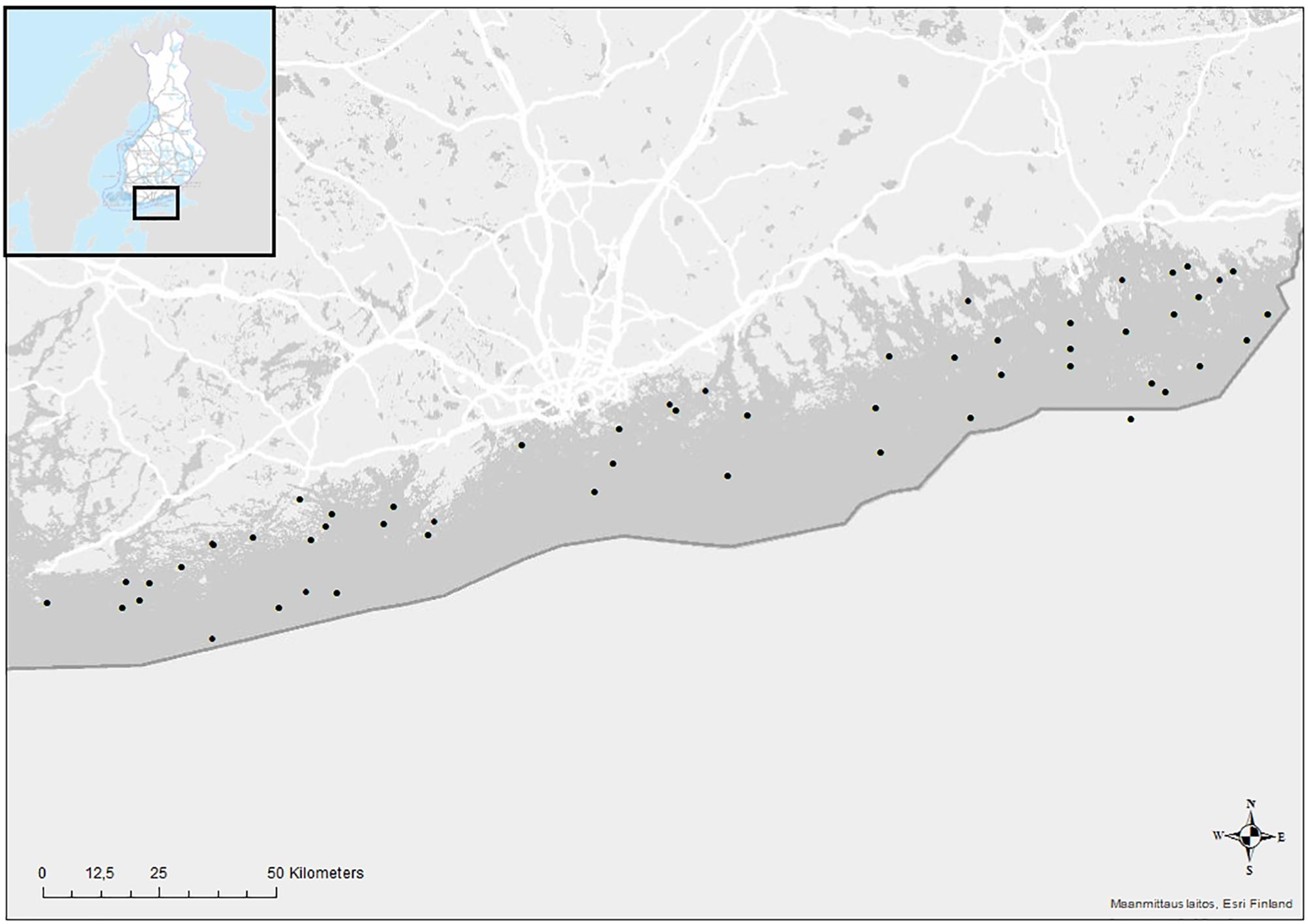
Figure 1. Map of the study area and the sampling stations in the Finnish coast of the Gulf of Finland, the Baltic Sea.

The Finnish monitoring program for the coastal macrozoobenthos has been carried out in the GoF since 2001. The benthos samples typically include only a few species due to frequent periods of hypoxia and of the brackish-water conditions of the study area, where many marine and freshwater species live on the edges of their distribution range. For this study, 55 zoobenthic sampling stations were chosen as these included measurements of oxygen, temperature, salinity, total phosphorus and total nitrogen. Samples with no observed macrofaunal life were also included in the study.

Sampling of Zoobenthos

Zoobenthos was sampled using the coastal research vessel R/V Muikku. One quantitative benthic sample was taken at each station during each sampling event. The sample was taken using a van Veen grab sampler, with grab area of 0.1 m². The sediment consistency (%) of each van Veen sample was visually evaluated, and sediment types were determined according to the Wentworth (1922) classification method into small stones (pebbles), gravel, sand, silt, mud, and clay (mud had the same grain size as clay, but its organic material consistency was higher). Samples were sieved on a 1 mm mesh, and the sediment remains and animals were stored in 70% alcohol for further analysis in the laboratory. Each of the sampling stations was characterized by east-west location (longitude), seabed depth (meters), and location in a coastal gradient (inner archipelago, outer archipelago, open sea).

Water Quality

The water quality in the study area has been measured by regional ELY-centres and by FEI. Available data on oxygen, temperature, salinity, total phosphorus and total nitrogen, at less than 1 m above the bottom, was compiled for the study period. Possible effects of the chosen water quality variables (oxygen, total phosphorus, total nitrogen, salinity, and temperature) on zoobenthos were studied both coinciding with the timing of zoobenthic sampling, and using a 1 year time-lag between the environmental conditions and the fauna, as the preceding year may have affected the juvenile phases of the zoobenthos, which may still be visible in the samples of the following year. Hence, the study period for the environmental factors also included the year 2000. The concentration of oxygen (mg L^–1) was determined by the Winkler titration method, salinity was determined by conductometric titration and total phosphorus (μg L^–1) and total nitrogen (μg L^–1) were determined using spectrophotometry (Creative Commons/ELY-centres and FEI).

Statistical Analyses

In total, 523 samples of zoobenthos were included in the study, with eleven distinct taxa representative enough to be included in the species-specific analyses (there were few more species observed occasionally, but they occurred in less than 2% of the samples, and were thus omitted): the bivalve Limecola (Macoma) balthica; the gastropod Hydrobia spp.; the crustaceans Monoporeia affinis, Pontoporeia femorata, Gammarus spp. and Saduria entomon; the polychaetes Marenzelleria spp., Bylgides sarsi and Hediste diversicolor; the priapulid Halicryptus spinulosus, and chironomid larvae of the family Chironomidae (Diptera). Environmental factors used to explain the variation of zoobenthos in the analyses were depth (continuous), year (continuous), longitude (continuous), coastal gradient (categorized: inner archipelago, outer archipelago, open sea), sediment types (separately as dummy variables: small stones, gravel, sand, silt, mud, clay), total phosphorus (continuous), total phosphorus in the preceding year (continuous), total nitrogen (continuous), total nitrogen in the preceding year (continuous), oxygen content (continuous and categorized), oxygen content in the preceding year (continuous and categorized), temperature (continuous), temperature in the preceding year (continuous), salinity (continuous) and salinity in the preceding year (continuous).

The Plymouth Routines in Multivariate Ecological Research (PRIMER 6.0) was used to conduct the Multidimensional scaling (MDS), the SIMPROF-test with the cluster dendrogram, the BEST-analysis, and the similarity percentages (SIMPER) analysis (Clarke and Gorley, 2006). The species matrix was log-transformed [Log(X + 1)] and the environmental variables were normalized for all of the analyses, and a resemblance matrix (measuring resemblance between every pair of samples), using Bray Curtis distance measure, by variables (taxa) of the community data was used to conduct the MDS -analysis and the SIMPROF-test. A second resemblance matrix (using Euclidean distance) was created based on environmental data per stations and used for SIMPER and BEST-analyses.

Multidimensional scaling and SIMPROF-test were used to investigate the association of zoobenthic species in space and time. The analyses were conducted on the resemblance matrix (using Bray Curtis distance), based on the abundance log-transformed data. In order to investigate how the zoobenthic species were distributed in multidimensional space, and whether there was any specific structure in the community data (i.e., whether the studied taxa formed assemblages, sharing habitats), we first conducted an MDS run and the SIMPROF-test with Bray-Curtis similarity procedure, and then visualized the results (Clarke and Gorley, 2006). MDS represents the studied taxa as points in a 2-dimensional space based on their ecological similarity (distances) (Clarke and Gorley, 2006). SIMPROF-test examines if there is statistically significant evidence of clusters in the species data; the output is a dendrogram displaying the grouping of taxa into decreasing number of clusters based on their ecological similarity (Clarke and Gorley, 2006).

As oxygen at the seabed is prerequisite for benthic life, and species have differing tolerances to oxygen deficiency (see e.g., Vaquer-Sunyer and Duarte, 2008), we carried out a SIMPER -analysis to specifically analyse the assemblage structure in distinct oxygen categories. Oxygen was classified into 10 different categories (1 = 0–1, 2 = 1–2, 3 = 2–3, 4 = 3–4, 5 = 4–5, 6 = 5–6, 7 = 6–7, 8 = 7–8, 9 = 8–9, 10 = 9–10 mg L^–1). To further visualize the impact of O₂ on zoobenthos abundance patterns, each studied species was measured against O₂ to investigate whether the abundance of species was related to O₂.

The BEST-analysis, which is based on Euclidean distance measures, was conducted to investigate which variables of the spatial and temporal environmental factors and their combinations that “best” matched the observed assemblage structure. The BEST-routine maximized rank correlations between environmental and biotic matrices to identify environmental variables that accounted for the highest proportion of variation among benthic assemblages (Clarke et al., 2008). All of the environmental variables were included to investigate which of the variables or their combinations significantly correlated with the observed assemblage pattern. The Best analysis was used to supplement the CCA-analysis. The analysis searches over subsets of abiotic variables for a combination that optimizes the match between assemblages and associated environmental variables (Clarke and Gorley, 2006).

The R statistical language with vegan library was used to conduct Constrained Correspondence Analysis (CCA) to study the specific influence of the chosen environmental variables on the zoobenthic species (Oksanen et al., 2018). CCA catches only the variation which can be explained by the chosen environmental variables or constraints. The analysis is based on chi-square distances and conducts weighted linear mapping (Legendre and Legendre, 2012; Oksanen et al., 2018). The species matrix was log-transformed [Log(X+1)] for the analysis. The first analysis was run using all of the environmental variables. In addition, one more analysis was run excluding the variables which strongly correlated with salinity, namely depth, longitude, temperature and the archipelago gradient (inner, outer, open sea). The included variables in this second analysis were year, mud, clay, sand, gravel, oxygen concentration during the same year and the preceding year, phosphorus during the same and the preceding year, nitrogen during the same and the preceding year and salinity during the same and the preceding year.

The R statistical language with “MASS” library was used to fit Gaussian generalized linear models (GLM) with species, in order to find out the effect of chosen predictor variables (the same variables as in BEST and CCA) on individual species abundance patterns (Venables and Ripley, 2002). GLM is a linear regression method that allows for response variables that have non-normal distributions (Venables and Ripley, 2002).

Results

Similarity of Species in an Environmental Space

The MDS-ordination and the SIMPROF-test with the cluster dendrogram showed the similarity of species distribution in an environmental space (Figures 2, 3 and Table 1). H. spinulosus and Hydrobia spp., as well as S. entomon and M. affinis were likely to co-occur in the study area. In addition, Limecola (Macoma) balthica, M. affinis and S. entomon often shared habitats together. Furthermore H. diversicolor, H. spinulosus and Hydrobia spp. formed a cluster with each other. P. femorata and B. sarsi formed a cluster. Marenzelleria spp., Limecola balthica, S. entomon and M. affinis also formed a cluster together Figure 3 and Table 1. According to the results, only clusters formed by B. sarsi and P. femorata as well as Gammarus spp. and Chironomidae were non-significant. Chironomidae displayed a unique ecological niche, and they did not have high similarity with any other species. In addition, the stations with no observed macrofaunal species present (severe hypoxia or anoxia) were clearly different from the stations with species.

FIGURE 2

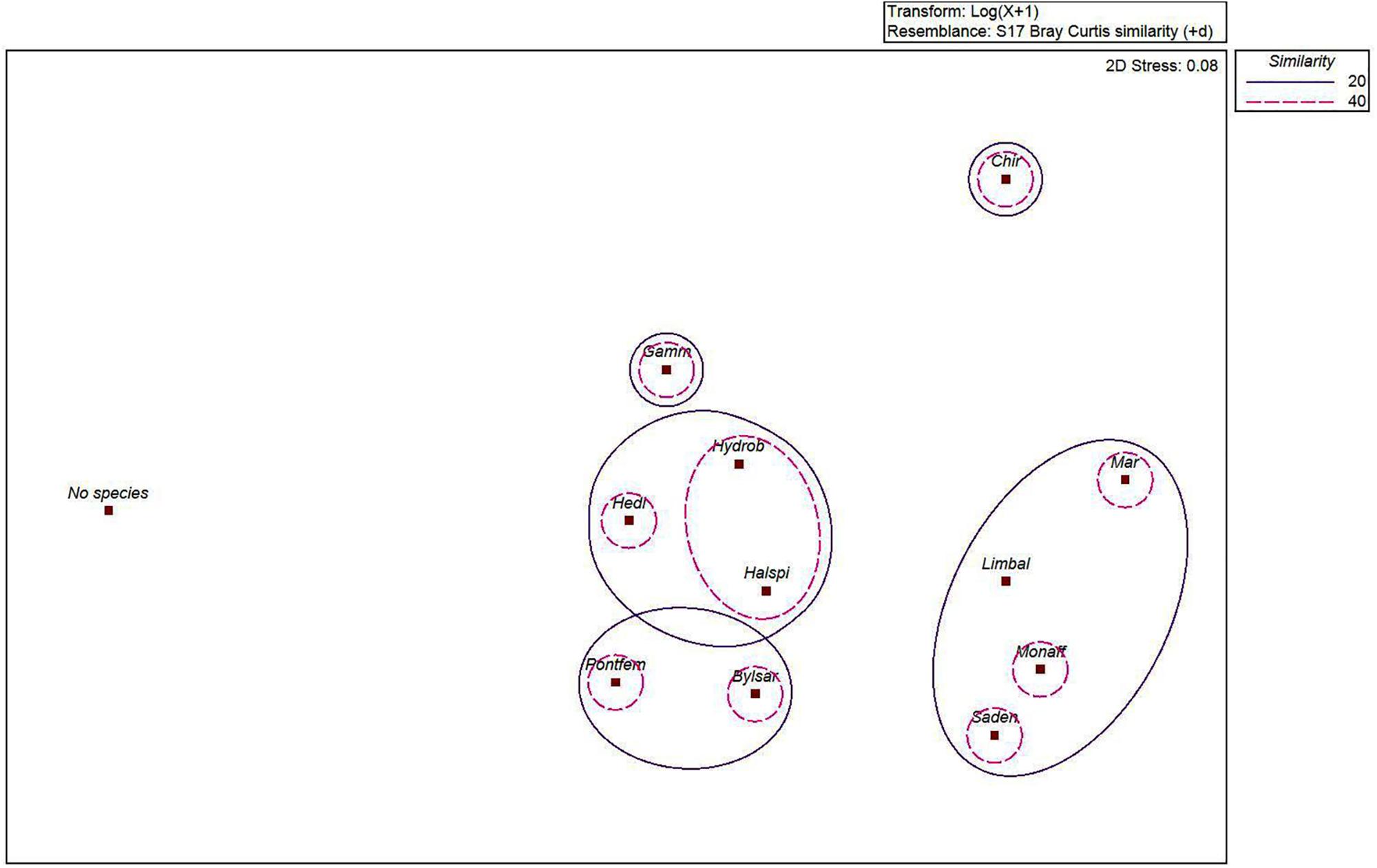
Figure 2. MDS-ordination on the similarity of the species (Marenzelleria spp., Bylgides sarsi, Hediste diversicolor, Halicryptus spinulosus, Limecola (Macoma) balthica, Hydrobia spp., Saduria entomon, Monoporeia affinis, Pontoporeia femorata, Gammarus spp., Chironomidae and variable “No species” (referring to samples lacking macrofaunal specimens) in an environmental space. 2D stress level of the test was 0.08, indicating sufficient statistical validity of the test. Bray Curtis similarity measure was used to define the similarity of species. Similarity levels of 20% (continuous line) and 40% (dashed line) are illustrated by contours.

FIGURE 3

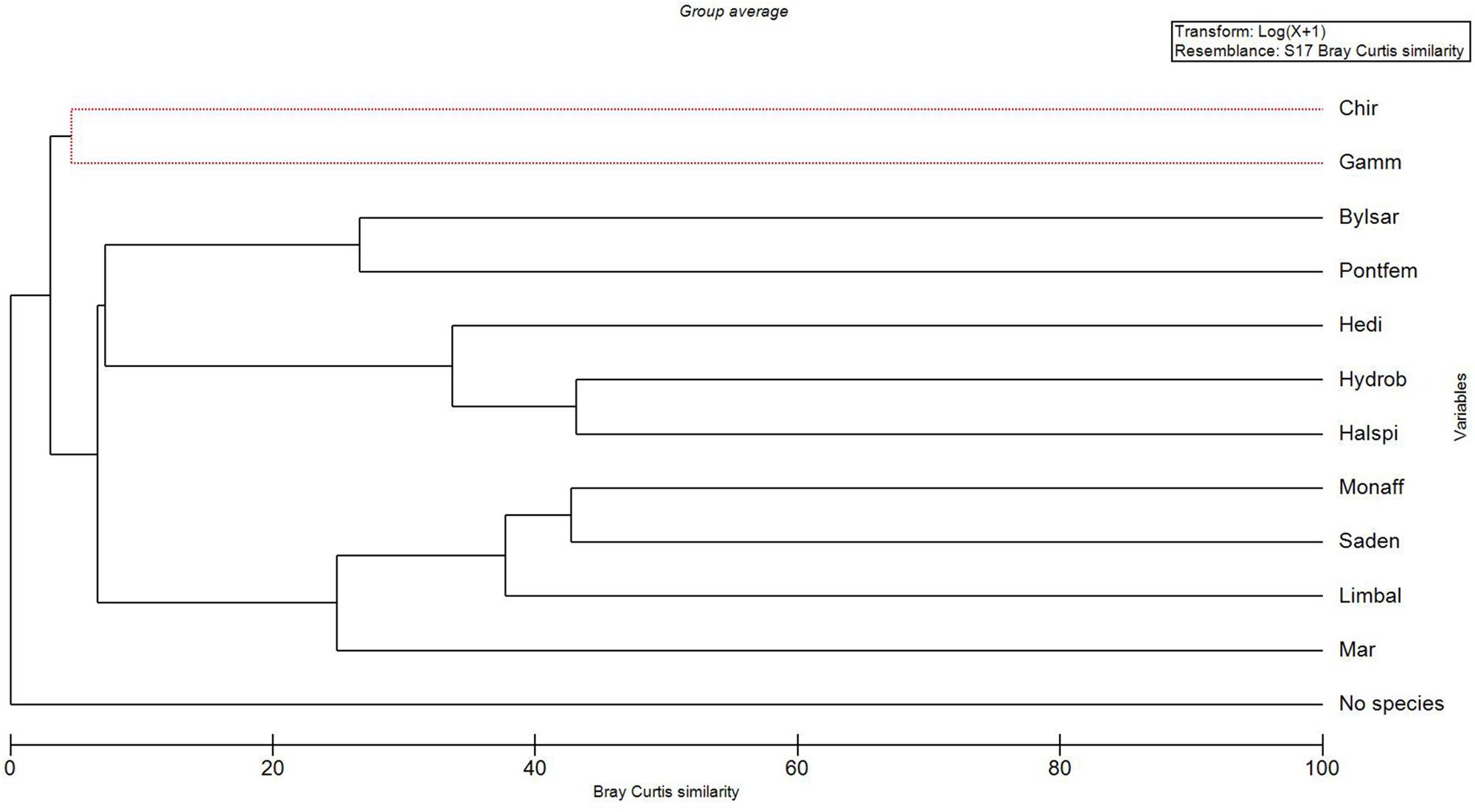
Figure 3. A cluster dendrogram output of the SIMPROF-test (see Table 1) with Bray Curtis similarity measure (x-axis) and variables (y-axis). “No species” refers to samples with lacking macro-benthic specimens. Taxa abbreviations: Mar – Marenzelleria spp., Limbal – Limecola (Macoma) balthica, Saden – Saduria entomon, Monaff – Monoporeia affinis, Hedi – Hediste diversicolor, Halspi – Halicryptus spinulosus, Hydrob = Hydrobia spp., Bylsar – Bylgides sarsi, Pontfem – Pontoporeia femorata, Gamm – Gammarus spp., Chir – Chironomidae. The red dashed lines refer to variables which cannot be significantly differentiated.

TABLE 1

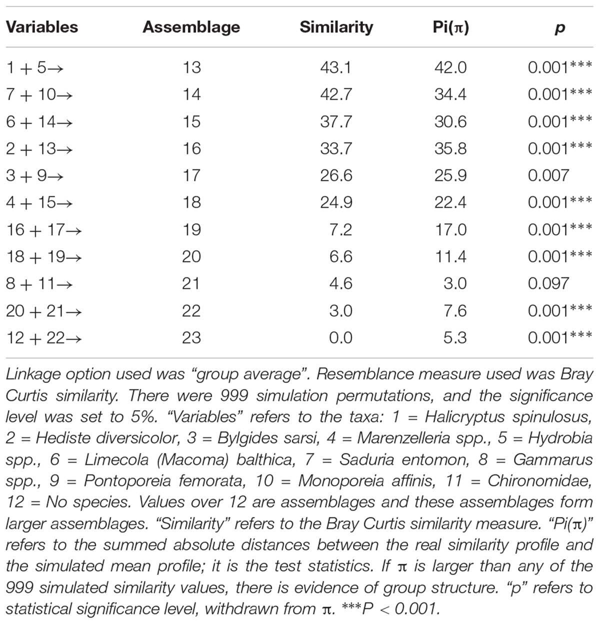
Table 1. SIMPROF-test results including relevant parameters. The results refer to the cluster diagram in Figure 3.

Effects of Environmental Variables on the Benthic Community Composition

The following significant correlations appeared between environmental variables: depth was correlated with archipelago gradient (r = 0.83), salinity (r = 0.72; illustrating the strong stratification in the Baltic Sea), temperature (r = −0.59) and nitrogen (r = −0.22). Nitrogen was also correlated with oxygen (r = −0.50) and phosphorus (r = 0.75). Phosphorus was also correlated with oxygen (r = −0.54). Archipelago gradient was also correlated with temperature (r = −0.55) and salinity (r = 0.63). Gravel was correlated with oxygen (r = 0.29). Salinity was also correlated with temperature (r = −0.59) and longitude (r = −0.24).

The CCA model was significant (p = 0.001, χ² = 1.07). Four of the first axes were significant; axis one (p = 0.001, χ² = 0.40), axis two (p = 0.001, χ² = 0.28), axis three (p = 0.005, χ² = 0.14) and axis four (p = 0.009, χ² = 0.12). The results showed that several driving factors significantly affected the species abundances in our study area (Table 2). In order of significance these were depth, longitude, year, mud, archipelago gradient, temperature of the previous year, clay, oxygen of the same and previous year (equal), temperature of the same year, total nitrogen of the same year, sand, total nitrogen of the previous year, and total phosphorus of the same year. All of the fore mentioned factors were statistically significant. Figure 4 illustrates the effect of the statistically significant variables on the studied zoobenthos.

TABLE 2

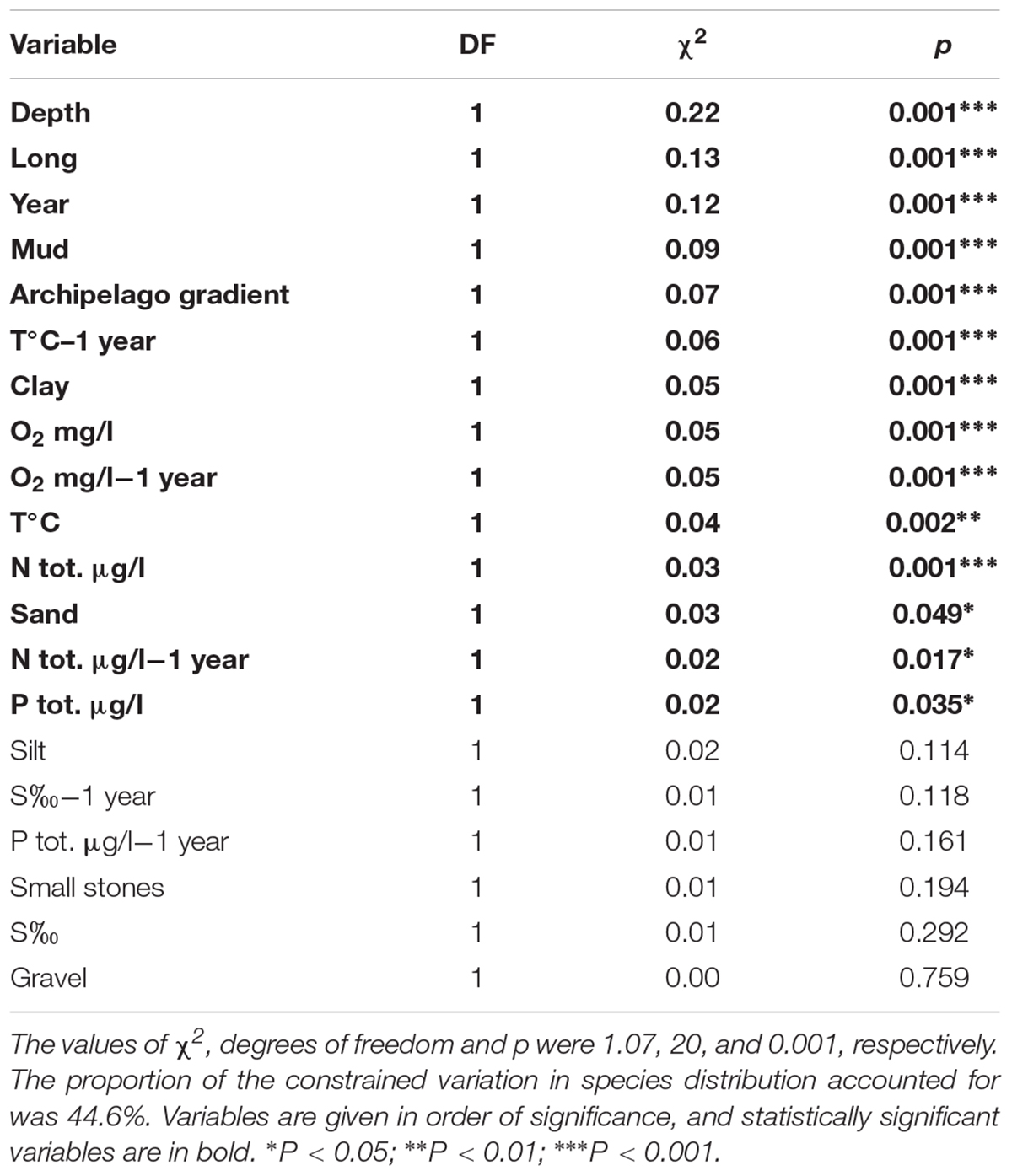
Table 2. The constrained variation and the statistical significance of the environmental variables used in the CCA –analysis, when all of the 20 variables were included.

FIGURE 4

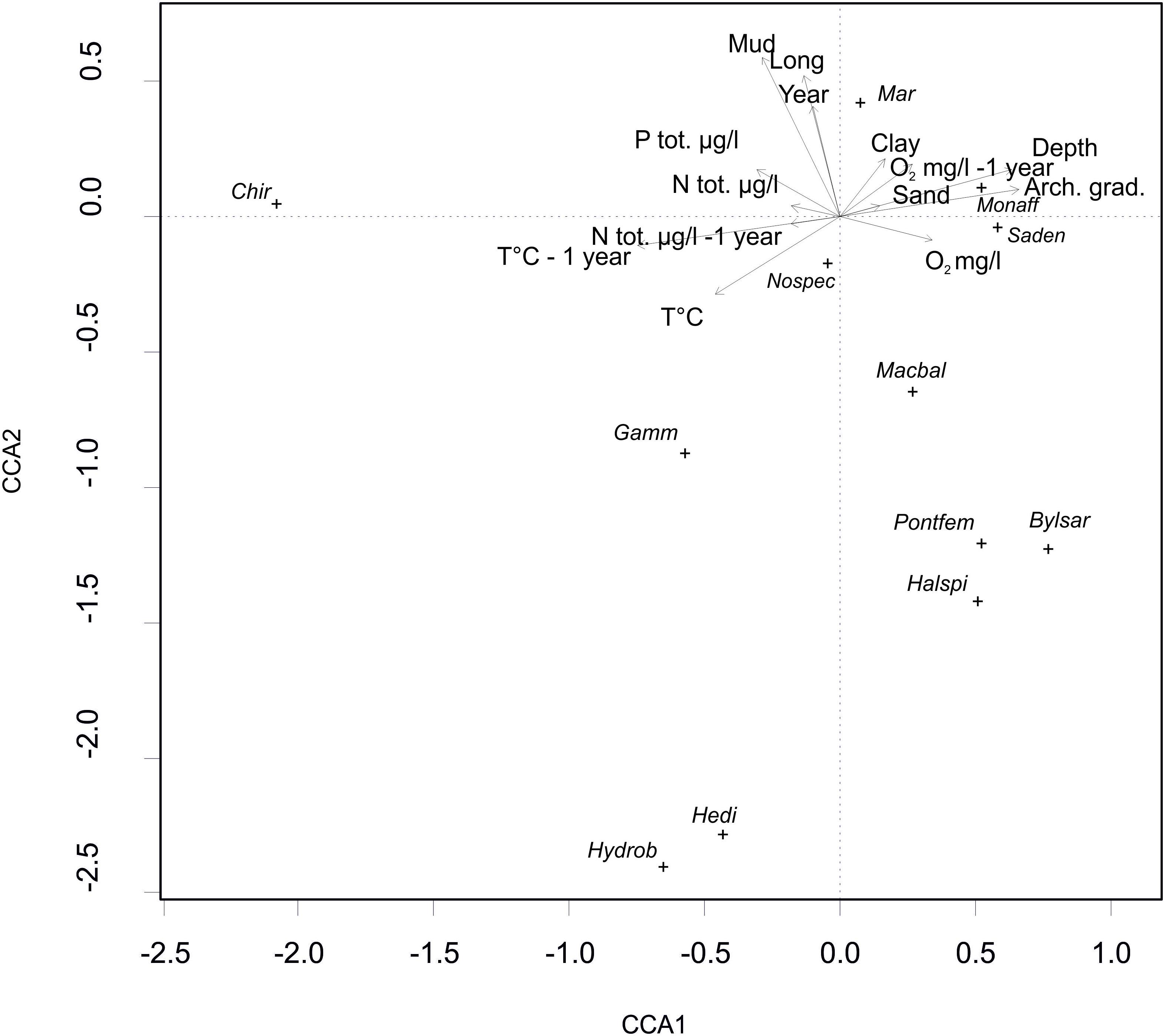
Figure 4. A CCA biplot depicting the effect of the statistically significant environmental variables (see Table 1), on the distribution and abundance of zoobenthic species (Mar – Marenzelleria spp., Bylsar – Bylgides sarsi, Halspi – Halicryptus spinulosus, Hedi – Hediste diversicolor, Gamm – Gammarus spp., Monaff – Monoporeia affinis, Pontfem – Pontoporeia femorata, Saden – Saduria entomon, Macbal – Limecola (Macoma) balthica, Hydrob – Hydrobia spp. Chir – Chironomidae).

When depth, archipelago gradient, temperature and longitude were omitted from the CCA (because of the strong correlation with salinity), the model was also significant (p = 0.001, χ² = 0.80). The four first axes were significant; axis one (p = 0.001, χ² = 0.31), axis two (p = 0.001, χ² = 0.23), axis three (p = 0.004, χ² = 0.10) and axis four (p = 0.010, χ² = 0.09). Salinity was the most significant variable in this analysis (p = 0.001, χ² = 0.14). In addition to salinity, mud (p = 0.001, χ² = 0.13), year (p = 0.001, χ² = 0.12), nitrogen of the same year (p = 0.001, χ²= 0.08), O₂ of the same year (p = 0.001, χ² = 0.08), O₂ of the previous year (p = 0.001, χ² = 0.06), clay (p = 0.002, χ² = 0.05), salinity of the previous year (p = 0.002, χ² = 0.03), and sand (p = 0.030, χ² = 0.03) were significant driving factors.

The CCA was supplemented with the BEST-analysis, which used Euclidean distances to find the “best” match between among-sample assemblage pattern and the related environmental factors driving it. The results indicated that sampling year, clay, silt, and sand had the highest Spearman rank correlation with the associated biotic matrix. The combined effect of these four variables accounted for 32% of the observed biological pattern.

Effects of Environmental Variables on the Species

The abundance of zoobenthos was differently affected by the studied environmental variables. In summary, the CCA results show that, Chironomidae was positively correlated with high temperatures and nutrient concentrations (Figure 4). Chironomidae also seemed to favor closeness to shore and relatively shallow depths with muddy sediments. Limecola (Macoma) balthica, B. sarsi, H. spinulosus and P. femorata were positively correlated with high O₂ concentrations. They were most abundant in the western parts of the study area in high salinity and during the earlier study years with less hypoxia present, but they did not favor muddy bottoms. The amphipods of the genus Gammarus seemed to favor high temperatures and high phosphorus content with 1 year’s time lag. The isopod S. entomon and the amphipod M. affinis were driven mostly by clayey or gravelly bottoms, and in addition occurred mostly in higher oxygen contents in deeper open sea stations. Marenzelleria occurred mostly in muddy bottoms during the later survey years and was most abundant in the eastern parts of the study area.

The GLM results (Supplementary Material 1) show that year (r = 0.096), clay (r = 0.134), mud (0.074) and oxygen content with a time lag of 1 year (0.061) significantly affected the abundance of Marenzelleria spp. Longitude (r = −0.000) and mud (r = −0.010) significantly affected the abundance of B. sarsi. Temperature (r = 0.008), mud (r = −0.008), total nitrogen with a time lag of 1 year (r = −0.000), and oxygen content with a time lag of 1 year (r = −0.007) significantly affected the abundance of H. diversicolor. Longitude (r = 0.000) significantly affected the abundance of H. spinulosus. Mud (r = −0.073), longitude (r = −0.000) and oxygen content (r = 0.031) significantly affected the abundance of Limecola (Macoma) balthica. Sand (r = 0.271), oxygen content (r = 0.027) and temperature with a time lag of 1 year (r = 0.031) significantly affected the abundance of S. entomon. Oxygen content (r = 0.047), year (r = 0.023), salinity with a time lag of 1 year (r = −0.129), clay (r = 0.045) and mud (r = −0.030) significantly affected the abundance of M. affinis. Mud (r = −0.008), year (r = 0.004) and longitude (r = −0.000) significantly affected the abundance of P. femorata. Mud (r = −0.014) and oxygen content with a time lag of 1 year (r = −0.011) significantly affected the abundance of Hydrobia spp. Temperature with a time lag of 1 year (r = 0.058), year (r = 0.028), total nitrogen (r = 0.001) and total phosphorus (r = −0.001) significantly affected the abundance of Chironomidae. In addition year (r = 0.079), longitude (r = −0.000), oxygen (r = 0.081) and sand (r = 0.349) significantly affected the number of species on the study sites. Gammarus spp. was the only taxon that did not significantly respond to the studied variables.

Distribution of Zoobenthos in Relation to Oxygen

The spatial distribution of the observed zoobenthic taxa was examined in relation to oxygen concentration (mg L^–1) at the time of the zoobenthic-sampling. Even if oxygen levels varied yearly and spatially, a pattern emerged that the number of species increased with the increasing O₂ concentration (Figure 5). Species-specific results show clear and specific adaptations to the gradient in oxygen levels (Figure 6). Pontoporeia femorata occurred at sites with O₂ concentrations of ≥6 mg L^–1. It was most abundant in areas with O₂ concentrations of around 8 mg L^–1 (up to < 70 ind. m^–2) and 6 mg L^–1 (∼ 48 ind. m^–2).

FIGURE 5

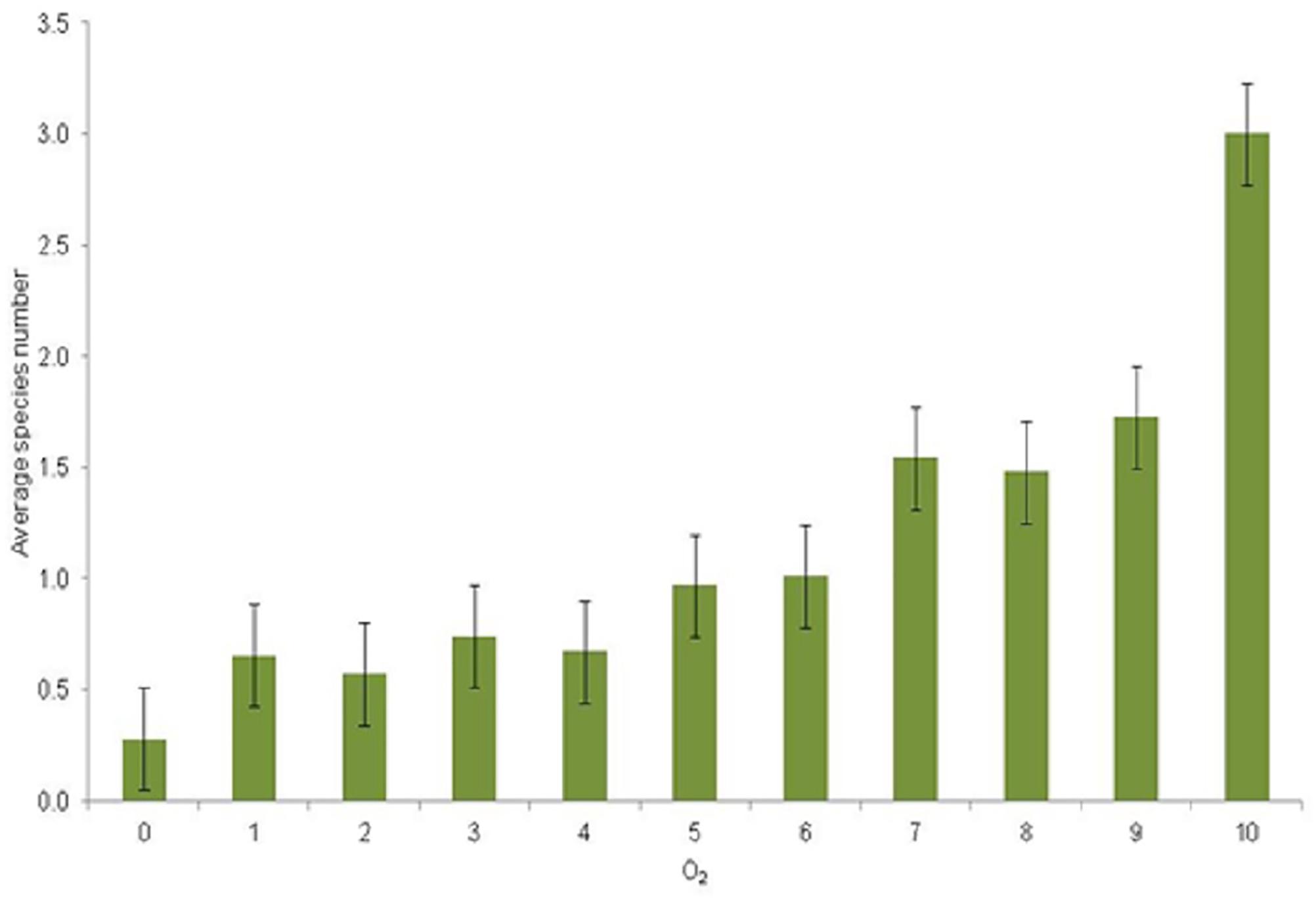
Figure 5. Average number of species (y-axis) per category of O₂ mg L^–1 (x-axis) and with standard error bars. Oxygen categories: 1 = 0–1, 2 = 1–2, 3 = 2–3, 4 = 3–4, 5 = 4–5, 6 = 5–6, 7 = 6–7, 8 = 7–8, 9 = 8–9, 10 = 9–10 mg L^–1.

FIGURE 6

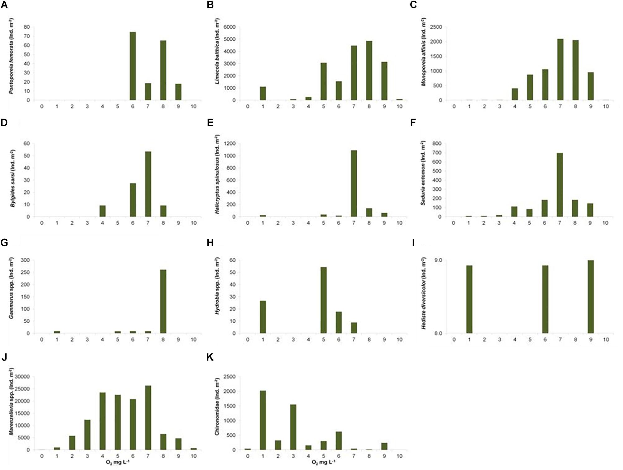
Figure 6. Total sum of studied taxa ind. m^–2 (y-axis) in distinct categories of O₂ mg L^–1 (x-axis). (A) Pontoporeia femorata, (B) Limecola (Macoma) balthica, (C) Monoporeia affinis, (D) Bylgides sarsi, (E) Halicryptus spinulosus, (F) Saduria entomon, (G) Gammarus spp., (H) Hydrobia spp., (I) Hediste diversicolor, (J) Marenzelleria spp., (K) Chironomidae.

Limecola (Macoma) balthica mainly occurred at sites with O₂ concentrations of ≥4 mg L^–1. It was most abundant in areas with O₂ concentrations of around 7 and 8 mg L^–1 (up to > 3400 ind. m^–2).

Monoporeia affinis mostly occurred at sites with O₂ concentrations of ≥4 mg L^–1. It was most abundant in areas with O₂ concentrations of around 7 and 8 mg L^–1 (up to 1690 ind. m^–2).

Bylgides sarsi was most abundant in 7 mg O₂ L^–1 (∼55 ind. m^–2). It was also present in O₂ concentrations of about 10 mg L^–1 (∼10 ind. m^–2). Its occurrence was not consistent along the oxygen gradient, as this species is mobile and tolerant to varying oxygen levels.

Halicryptus spinulosus was most abundant in 7–8 mg O₂ L^–1 (up to > 100 ind. m^–2). Although the species was totally absent in anoxic stations or in O₂ concentrations of 2–4 mg O₂ L^–1, it was randomly recorded in ∼1 mg O₂ L^–1 (up to ∼30 ind. m^–2).

Saduria entomon mostly occurred in areas with O₂ concentrations above 3 mg L^–1. It was most abundant at sites with O₂ concentrations of around 7 mg L^–1 (>420 ind. m^–2).

Gammarus spp. occurred in O₂ concentrations of around 5 mg L^–1 (∼10 ind. m^–2) and 8 mg L^–1 (∼250 ind. m^–2). It was totally absent in the sampling sites with O₂ concentrations of around 0, 2, 3, 4, and 9 mg L^–1, but was randomly found in O₂ concentrations of around 1, 6, and 7 mg L^–1.

Hydrobia spp. mostly occurred in O₂ concentrations of 5 mg L^–1 (∼ 50 ind. m^–2), but also randomly occurred in O₂ concentrations of 1, 6, and 7 mg L^–1.

The occurrence/distribution of H. diversicolor was random, with only a few individuals observed in the samples. It was found in O₂ concentrations of 9, 6, and 1 mg L^–1.

Marenzelleria spp. was most abundant (up to > 20000 ind. m^–2) in ca. 4 and 5 mg O₂ L^–1. The species was also relatively abundant around 6 and 7 mg O₂ L^–1 (up to > 15000 ind. m^–2). Marenzelleria was completely absent in anoxic stations but was randomly found in areas of very low oxygen concentration (1 mg O₂ L^–1).

Chironomidae occurred in all O₂ concentrations. However, it was most abundant in stations with low O₂ concentrations of around 1 mg L^–1 (>1000 ind. m^–2).

As a result of the SIMPER -analysis, characteristic assemblage compositions were described for each O₂ concentration -level (Table 3). Only Chironomidae and Marenzelleria were high in abundance in the lowest O₂ concentrations (0–1 and 1–2 mg L^–1). In concentrations of up to 5 mg L^–1 the assemblages were defined by Marenzelleria, Limecola (Macoma) balthica, S. entomon and Chironomidae. In O₂ concentrations of 6–9 mg L^–1 the assemblages were defined by Marenzelleria, S. entomon, M. affinis, Limecola (Macoma) balthica, B. sarsi, Chironomidae and H. spinulosus and these were also the most species-rich assemblages. The mean similarity of the sample communities decreased with higher O₂ concentrations and community diversity (Table 3).

TABLE 3

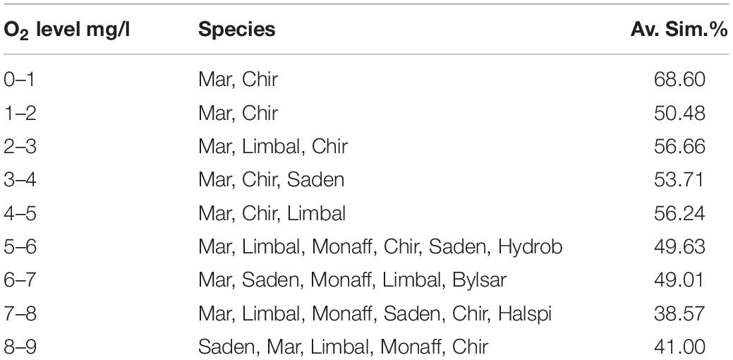
Table 3. Zoobenthic species contributing to the similarity of assemblages defined by O₂, and the average similarity (%) of assemblages in 9 different O₂ categories (0–1, 1–2, 2–3, 3–4, 4–5, 5–6, 6–7, 7–8, 8–9 mg L^–1; category 10 only included one species and was thus omitted).

Discussion

We found that the benthic species occurrence and abundance were primarily affected by depth (representing salinity and temperature, as both correlate with depth), east-west gradient (representing salinity), sampling year (temporal aspect), coastal zone (representing depth and closeness to shore; spatial aspect), seabed substrate (representing grain size and sediment organic content), and chemical factors (O₂ concentration, nitrogen concentration, phosphorus concentration and temperature). In support for our first hypothesis, the eutrophication process affects the zoobenthic assemblage composition: even if nutrient concentrations were significant explanatory variables, it was best manifested through the indirect secondary effects of eutrophication, i.e., changes (reductions) in oxygen concentration as a consequence of increased sedimentation of pelagic primary production and thus increased oxygen demand (Griffiths et al., 2017). As the sampling was temporally infrequent (annual), and the water chemical variables were not always measured during the same day as zoobenthic samples, it cannot be ruled out that higher levels of correlation and direct influence of the chosen environmental factors would have been seen closer to the zoobenthos sampling time (e.g., Weigel et al., 2015), although time-series studies with once-per-year sampling have proven to be fruitful before in this marine to brackish-water region (Rousi et al., 2013; Törnroos et al., 2019).

We were able to show relevant results with just one zoobenthic sample per station per year. Cuff and Coleman (1979) found that one sample with van Veen grab from a site was representative enough, provided the spatial coverage of sampling sites was sufficient, which was the basis for the sampling-design in our study. Our data is based on long-term coastal monitoring data, and the monitoring program is primarily designed for observing regional environmental changes. In support of the faunal samples, this study included information on sediment types, and there is a correlation between soft sediment (mud, soft clay and silt) and sediment organic content (e.g., Leipe et al., 2011; Hossain et al., 2014), i.e., the softer the sediment, the higher the organic content. Thus the factor “sediment type” in our study explains the part of the variability which can be associated with organic content.

The Environmental Variables Driving the Zoobenthos Abundance Trends in the GoF

Our results showed that both spatial and temporal variables accounted for the distribution of zoobenthos in the study area, the Finnish coastal region of the GoF (Figure 1). In support of our second hypothesis, the spatial variables (i.e., depth, east-west gradient) were more important than the temporal dynamics (sampling year) (Bonsdorff, 2006; Laine et al., 2007). According to the CCA-analysis, depth was the most important driver for the abundance of the zoobenthos; also longitude, year, mud, archipelago gradient, salinity, temperature, clay, oxygen, sand, and nutrients significantly affected zoobenthos distribution patterns. In the BEST-analysis, sampling year and the sediment-fraction clay accounted for most of the variation in abundance, but also sand and silt were significant drivers. The important role of substrate according to BEST was somewhat surprising as the sediments were mainly characterized as mud/clay, and a wider variety of substrates was not registered in the study area in spite of the large spatial scale of coverage over hundreds of kilometers (Figure 1). In contrast, Rousi et al. (2011) showed that spatial heterogeneity in coastal soft-sediment systems can be high even over small spatial scales in complex and mosaic archipelago areas. This classification of the substrates into gravel, sand, mud and clay is in line with the biotope definitions made in the Baltic Sea (HELCOM, 2013), and shows that assessments of the state of the substrate-based benthic biotopes can be done by coastal zoobenthic monitoring programs. Such an assessment is also required as part of the EU MSFD (EU-COM, 2017).

The BEST-analysis, which used Euclidean distance measure between environmental variables and zoobenthos, differed clearly from the CCA -analysis which used Chi-square distances between the environmental variables and respective zoobenthic assemblages. Euclidean distance is based on geometry, and Chi-square distance is based on differences between objects in the proportional representation of the species (Quinn and Keough, 2002). Canonical partitioning such as CCA is more suitable when studying community composition among sites, because it correctly estimates the different portions of community composition variation, whereas geometric distance underestimates the variation explained by environmental variables (Legendre et al., 2005).

Zoobenthos as an Integrative Indicator of Human Impacts

The monitoring and assessment of zoobenthos is part of the national Finnish program in support of EU water and marine policies (EU WFD and EU MSFD). The assessments provide advice on the level of human impacts on the marine and coastal environment, and are used to justify management measures. According to our results, the zoobenthos respond species-specifically to temporal oxygen deficiency, which is driven by regional coastal eutrophication and dynamics between offshore hypoxic areas and the coast. In addition, nutrient concentrations in the sampling area significantly affected the community composition. Even though the response to total phosphorus and nitrogen concentrations can also indicate an indirect effect reflecting the more general level of eutrophication, these factors give sufficient evidence that zoobenthic assemblages are good environmental indicators for eutrophication assessments in combination with physical and chemical environmental drivers (Villnäs and Norkko, 2011). Similar results have been shown for many coastal areas in Europe and other parts of the world (e.g., Zimboura and Zenetos, 2002; Bonsdorff et al., 2003; Cardoso et al., 2007; Perus et al., 2007; Foden et al., 2011; Howarth et al., 2011, and Snickars et al., 2014). The effects of oxygen, salinity and temperature on the zoobenthos have also been studied in the open sea area of the GoF by Laine et al. (1997, 2007), and the results from these deeper areas more frequently experiencing hypoxia support our findings. Our study highlights the temporal and spatial effects of nutrients and oxygen in the coastal Gulf of Finland, which is directly influenced by local nutrient loading and the fluctuating waters of the adjacent deep Baltic Proper, and the highly stressed coastal systems of the innermost parts of the gulf (Maximov et al., 2015).

Climate change-related variables, such as increasing temperature and reduced salinity in estuarine environments, have been shown to impact the distribution patterns of zoobenthos (e.g., Vaquer-Sunyer and Duarte, 2008; Rousi et al., 2013; Snickars et al., 2014; Grebmeier et al., 2015). We found implications of the significant effects of temperature and salinity on several of the studied species. Long-term and large-scale severe eutrophication may also be enhanced by both climate change-induced increases in precipitation and subsequent runoff of nutrients from land (Diaz and Rosenberg, 2008), and due to higher oxygen demand in the sedimentary systems in response to increased temperature (Vaquer-Sunyer and Duarte, 2008). On a larger scale, the basic changes seen in the GoF mirror those recorded along the entire Baltic Sea gradient (Andersen et al., 2017; Reusch et al., 2018), where the zoobenthos forms a continuum of gradual change dictated by the natural environmental gradients and amplified by eutrophication, oxygen deficiency and global change-related factors (Rumohr et al., 1996; Bonsdorff and Pearson, 1999; Bonsdorff, 2006; Gogina et al., 2016).

The Role of Oxygen in Shaping the Zoobenthic Assemblages

Along with biotic factors, such as ambient population dynamics, recolonization of benthic habitats after disturbance is dependent on abiotic factors of the surrounding areas (Zajac and Whitlatch, 1982). Our results clearly show that oxygen (normoxia, hypoxia, anoxia) is a strong predictor for species diversity and occurrence in the zoobenthic assemblage. Different taxa have specific tolerance ranges which can be predicted from the oxygen measurements in the same year and the previous year. This suggests that zoobenthic indicators can describe and mirror the benthic physical and chemical conditions over longer time spans even if the O₂ conditions have likely fluctuated during the period, which is in support of our third hypothesis.

The analysis showed that only the larvae of dipteran chironomids were well adapted to live in very low O₂ conditions (all the other recorded benthic species thrived in higher O₂ concentrations) as their tolerance to oxygen deficiency is evidently better, in part due to their high oxygen-binding capacity in response to their high levels of hemoglobin (Ha and Choi, 2008).

We conclude that the zoobenthos monitoring of the outer coastal waters of the GoF supports the assessments of the state of marine environment and that the zoobenthic assemblages are influenced by not only the sedimentary substrates but also variables related to eutrophication, closeness to shore, salinity and water temperature. Oxygen is one of the main environmental variables shaping the species composition, and we showed how species richness declined in the relatively species-poor benthic community as oxygen declined.

Data Availability

The raw data supporting the conclusions of this manuscript will be made available by the authors, without undue reservation, to any qualified researcher.

Author Contributions

HR was responsible for the research. HR and SK performed the statistical analyses. All authors planned the research and wrote the manuscript.

Funding

This study was supported by the Åbo Akademi University Foundation (to EB).

Conflict of Interest Statement

The authors declare that the research was conducted in the absence of any commercial or financial relationships that could be construed as a potential conflict of interest.

Acknowledgments

We want to thank the Finnish Environment administration (FEI and ELY-centre) for collecting the data. We also want to thank the R/V Muikku crew, and all those who participated in the data collection and analysis. Furthermore, we want to thank the Åbo Akademi University, and especially Dr. Katri Aarnio for some previously undone zoobenthic species laboratory analyses. We also want to thank the editor SC and the two reviewers for their big help in improving the manuscript. Over-inspector Mikaela Ahlman (ELY-centre) is thanked for her comments in an earlier version of the manuscript. The Åbo Akademi University Foundation is thanked for financial support (EB).

Supplementary Material

The Supplementary Material for this article can be found online at: https://www.frontiersin.org/articles/10.3389/fmars.2019.00464/full#supplementary-material

References

Alenius, P., Myrberg, K., and Nekrasov, A. (1998). The physical oceanography of the Gulf of Finland: a review. Bor. Environ. Res. 3, 97–125.

Google Scholar

Andersen, J. H., Carstensen, J., Conley, D. J., Dromph, K., Fleming-Lehtinen, V., Gustafsson, B. G., et al. (2017). Long-term temporal and spatial trends in eutrophication status of the Baltic Sea. Biol. Rev. 92, 135–149. doi: 10.1111/brv.12221

PubMed Abstract | CrossRef Full Text | Google Scholar

Bonsdorff, E. (2006). Zoobenthic diversity-gradients in the Baltic Sea: continuous post-glacial succession in a stressed ecosystem. J. Exp. Mar. Biol. Ecol. 330, 383–391. doi: 10.1016/j.jembe.2005.12.041

CrossRef Full Text | Google Scholar

Bonsdorff, E., Blomqvist, E. M., Mattila, J., and Norkko, A. (1997). Coastal eutrophication: causes, consequences and perspectives in the archipelago areas of the northern Baltic Sea. Estuar. Coast. Shelf Sci. 44, 63–72. doi: 10.1016/s0272-7714(97)80008-x

CrossRef Full Text | Google Scholar

Bonsdorff, E., Laine, A. O., Hänninen, J., Vuorinen, I., and Norkko, A. (2003). Zoobenthos of the outer archipelago waters (N. Baltic Sea) – the importance of local conditions for spatial distribution patterns. Bor. Environ. Res. 8, 135–145.

Google Scholar

Bonsdorff, E., and Pearson, T. H. (1999). Variation in the sublittoral macrozoobenthos of the Baltic Sea along environmental gradients; a functional-group approach. Aust. J. Ecol. 24, 312–326. doi: 10.1046/j.1442-9993.1999.00986.x

CrossRef Full Text | Google Scholar

Cardoso, P. G., Bankovic, M., Raffaelli, D., and Pardal, M. A. (2007). Polychaete assemblages as indicators of habitat recovery in a temperate estuary under eutrophication. Estuar. Coast. Shelf Sci. 71, 301–308. doi: 10.1016/j.ecss.2006.08.002

CrossRef Full Text | Google Scholar

Carstensen, J., Andersen, J. H., Gustafsson, B. G., and Conley, D. J. (2014). Deoxygenation of the Baltic Sea during the last century. Proc. Natl. Acad. Sci. U.S.A. 111, 5628–5633. doi: 10.1073/pnas.1323156111

PubMed Abstract | CrossRef Full Text | Google Scholar

Clarke, K. R., and Gorley, R. N. (2006). PRIMER. Plymouth: Primer-E.

Google Scholar

Clarke, K. R., Somerfield, P. J., and Gorley, R. N. (2008). Testing of null hypotheses in exploratory community analyses: similarity profiles and biota-environment linkage. J. Exp. Mar. Biol. Ecol. 366, 56–69. doi: 10.1016/j.jembe.2008.07.009

CrossRef Full Text | Google Scholar

Conley, D. J., Carstensen, J., Aigars, J., Axe, P., Bonsdorff, E., Eremina, T., et al. (2011). Hypoxia is increasing in the coastal zone of the Baltic Sea. Environ. Sci. Technol. 45, 6777–6783. doi: 10.1021/es201212r

PubMed Abstract | CrossRef Full Text | Google Scholar

Cuff, W., and Coleman, N. (1979). Optimal survey design: lessons from a stratified random sample of macrobenthos. J. Fish. Res. Board Can. 36, 351–361. doi: 10.1139/f79-054

CrossRef Full Text | Google Scholar

Diaz, R. J., and Rosenberg, R. (2008). Spreading dead zones and consequences for marine ecosystems. Science 321, 926–929. doi: 10.1126/science.1156401

PubMed Abstract | CrossRef Full Text | Google Scholar

EU-COM (2017). Commission Decision (EU) 2017/848 of 17 May 2017 Laying Down Criteria and Methodological Standards on Good Environmental Status of Marine Waters and Specifications and Standardized Methods for Monitoring and Assessment, and Repealing Decision 2010/477/EU. Brussels: European Commission.

Google Scholar

Foden, J., Devlin, M. J., Mills, D. K., and Malcolm, S. J. (2011). Searching for undesirable disturbance: an application of the OSPAR eutrophication assessment method to marine waters of England and Wales. Biogeochemistry 106, 157–175. doi: 10.1007/s10533-010-9475-9

CrossRef Full Text | Google Scholar

Gogina, M., Nygård, H., Blomqvist, M., Daunys, D., Josefson, A. B., Kotta, J., et al. (2016). The Baltic Sea scale inventory of benthic faunal communities. ICES J. Mar. Sci. 73, 1196–1213. doi: 10.1093/icesjms/fsv265

CrossRef Full Text | Google Scholar

Grebmeier, J. M., Bluhm, B. A., Cooper, L. W., Denisenko, S. G., Iken, K., Kȩdra, M., et al. (2015). Time-series benthic community composition and biomass and associated environmental characteristics in the Chukchi Sea during the RUSALCA 2004–2012 program. Oceanography 28, 116–133. doi: 10.5670/oceanog.2015.61

CrossRef Full Text | Google Scholar

Griffiths, J. R., Kadin, M., Nascimento, F. J. A., Tamelander, T., Törnroos, A., Bonaglia, S., et al. (2017). The importance of benthic-pelagic coupling for marine ecosystem functioning in a changing world. Glob. Change Biol. 23, 2179–2196. doi: 10.1111/gcb.13642

PubMed Abstract | CrossRef Full Text | Google Scholar

Ha, M. H., and Choi, J. (2008). Effects of environmental contaminants on hemoglobin of larvae of aquatic midge, Chironomus riparius (Diptera: Chironomidae): a potential biomarker for ecotoxicity monitoring. Chemosphere 71, 1928–1936. doi: 10.1016/j.chemosphere.2008.01.018

PubMed Abstract | CrossRef Full Text | Google Scholar

Heiskanen, A. S., Bonsdorff, E., and Joas, M. (2019). “Baltic Sea: a recovering future from decades of eutrophication,” in Coasts and Estuaries. The Future, eds E. Wolanski, J. W. Day, M. Elliott, and R. Ramachandran (Amsterdam: Elsevier), 343–362. doi: 10.1016/b978-0-12-814003-1.00020-4

CrossRef Full Text | Google Scholar

HELCOM (2009). Eutrophication in the Baltic Sea. An Integrated Thematic Assessment of the Effects of Nutrient Enrichment in the Baltic Sea Region. Helsinki: Helsinki Commission. doi: 10.13140/RG.2.1.2669.0400

CrossRef Full Text | Google Scholar

HELCOM (2013). Technical Report on the HELCOM Underwater Biotope and Habitat Classification. Helsinki: Helsinki Commission.

Google Scholar

HELCOM (2018). State of the Baltic Sea – Second HELCOM Holistic Assessment 2011–2016. Available at: http://stateofthebalticsea.helcom.fi/ (accessed November 13, 2018).

Google Scholar

Hossain, M. B., Marshall, D. J., and Senaphati, V. (2014). Sediment granulometry and organic matter content in the intertidal zone of the Sungai Brunei estuarine system, northwest coast of Borneo. Carpathian J. Earth Environ. Sci. 9, 231–239.

Google Scholar

Howarth, R., Chan, F., Conley, D. J., Garnier, J., Doney, S. C., Marino, R., et al. (2011). Coupled biogeochemical cycles: eutrophication and hypoxia in temperate estuaries and coastal marine ecosystems. Front. Ecol. Environ. 9, 18–26. doi: 10.2307/41149673

CrossRef Full Text | Google Scholar

Laine, A. O. (2003). Distribution of soft-bottom macrofauna in the deep open Baltic Sea in relation to environmental variability. Estuar. Coast. Shelf. Sci. 57, 87–97. doi: 10.1016/s0272-7714(02)00333-5

CrossRef Full Text | Google Scholar

Laine, A. O., Andersin, A. B., Leiniö, S., and Zuur, A. F. (2007). Stratification induced hypoxia as a structuring factor of macrozoobenthos in the Open Gulf of Finland (Baltic Sea). J. Sea Res. 57, 65–77. doi: 10.1016/j.seares.2006.08.003

CrossRef Full Text | Google Scholar

Laine, A. O., Sandler, H., Andersin, A. B., and Stigzelius, J. (1997). Long-term changes of macrozoobenthos in the eastern gotland basin and the gulf of Finland (Baltic Sea) in relation to the hydrographical regime. J. Sea Res. 38, 135–159. doi: 10.1016/s1385-1101(97)00034-8

CrossRef Full Text | Google Scholar

Legendre, P., Borcard, D., and Peres-Neto, P. R. (2005). Analyzing Beta diversity: partitioning the spatial variation of community composition data. Ecol. Monogr. 75, 435–450. doi: 10.1890/05-0549

CrossRef Full Text | Google Scholar

Legendre, P., and Legendre, L. (2012). Complex ecological data sets. Dev. Environ. Model. 24, 1–57. doi: 10.1016/b978-0-444-53868-0.50001-0

CrossRef Full Text | Google Scholar

Leipe, T., Tauber, F., Vallius, H., Virtasalo, J., Uscinowicz, S., Kowalski, N., et al. (2011). Particulate organic carbon (POC) in surface sediments of the Baltic Sea. Geo Mar. Lett. 31, 175–188. doi: 10.1007/s00367-010-0223-x

CrossRef Full Text | Google Scholar

Leppäranta, M., and Myrberg, K. (2009). Physical Oceanography of the Baltic Sea. Heidelberg: Springer-Verlag.

Google Scholar

Lundberg, C., Lönnroth, M., von Numers, M., and Bonsdorff, E. (2005). A multivariate assessment of coastal eutrophication. Examples from the Gulf of Finland, northern Baltic Sea. Mar. Pollut. Bull. 50, 1185–1196. doi: 10.1016/j.marpolbul.2005.04.029

PubMed Abstract | CrossRef Full Text | Google Scholar

Maximov, A., Bonsdorff, E., Eremina, T., Kauppi, L., Norkko, A., and Norkko, J. (2015). Context-dependent consequences of Marenzelleria spp. (Spionidae: Polychaeta) invasion for nutrient cycling in the Northern Baltic Sea. Oceanologia 57, 342–348. doi: 10.1016/j.oceano.2015.06.002

CrossRef Full Text | Google Scholar

Oksanen, J., Blanchet, F. G., Friendly, M., Kindt, R., Legendre, P., McGlinn, D., et al. (2018). Community Ecology Package. Available at: https://cran.r-project.org/ (accessed March 5, 2019).

Google Scholar

Perus, J., Bonsdorff, E., Bäck, S., Lax, H.-G., Villnäs, A., and Westberg, V. (2007). Zoobenthos as indicators of ecological status in coastal brackish waters: a comparative study from the Baltic Sea. Ambio 36, 250–256. doi: 10.1579/0044-7447(2007)36

PubMed Abstract | CrossRef Full Text | Google Scholar

Quinn, G. P., and Keough, M. J. (2002). Experimental Design and Data Analysis for Biologists. Cambridge: Cambridge University Press. doi: 10.1017/CBO9780511806384

CrossRef Full Text | Google Scholar

Raateoja, M., and Setälä, O. (2016). The Gulf of Finland Assessment. Reports of the Finnish Environment Institute 27. Available at: http://hdl.handle.net/10138/166296 (accessed May 7, 2019).

Google Scholar

Reusch, T. B. H., Dierking, J., Andersson, H. C., Bonsdorff, E., Carstensen, J., Casini, M., et al. (2018). The Baltic Sea as a time machine for the future coastal ocean. Sci. Adv. 4:eaar8195. doi: 10.1126/sciadv.aar8195

PubMed Abstract | CrossRef Full Text | Google Scholar

Rönnberg, C., and Bonsdorff, E. (2004). Baltic Sea eutrophication: area-specific ecological consequences. Hydrobiologia 514, 227–241. doi: 10.1007/978-94-017-0920-0_21

CrossRef Full Text | Google Scholar

Rousi, H., Laine, A. O., Peltonen, H., Kangas, P., Andersin, A. B., Rissanen, J., et al. (2013). Long-term changes in coastal zoobenthos in the northern Baltic Sea: the role of abiotic environmental factors. ICES J. Mar. Sci. 70, 440–451. doi: 10.1093/icesjms/fss197

CrossRef Full Text | Google Scholar

Rousi, H., Peltonen, H., Mattila, J., Bäck, S., and Bonsdorff, E. (2011). Impacts of physical environmental characteristics on the distribution of benthic fauna in the northern Baltic Sea. Bor. Environ. Res. 16, 521–533.

Google Scholar

Rumohr, H., Bonsdorff, E., and Pearson, T. H. (1996). Zoobenthic succession in Baltic sedimentary habitats. Arch. Fish. Mar. Res. 44, 179–214.

Google Scholar

Snickars, M., Weigel, B., and Bonsdorff, E. (2014). Impact of eutrophication and climate change on fish and zoobenthos in coastal waters of the Baltic Sea. Mar. Biol. 162, 141–151. doi: 10.1007/s00227-014-2579-2573

CrossRef Full Text | Google Scholar

Törnroos, A., Pecuchet, L., Olsson, J., Gårdmark, A., Blomqvist, M., Lindegren, M., et al. (2019). Four decades of functional community change reveals gradual trends and low interlinkage across trophic groups in a large marine ecosystem. Glob. Change Biol. 25, 1235–1246. doi: 10.1111/gcb.14552

PubMed Abstract | CrossRef Full Text | Google Scholar

Vaquer-Sunyer, R., and Duarte, C. M. (2008). Thresholds of hypoxia for marine biodiversity. Proc. Natl. Acad. Sci. U.S.A. 105, 15452–15457. doi: 10.1073/pnas.0803833105

PubMed Abstract | CrossRef Full Text | Google Scholar

Venables, W. N., and Ripley, B. D. (2002). Modern Applied Statistics with S. New York, NY: Springer-Verlag.

Google Scholar

Villnäs, A., and Norkko, A. (2011). Benthic diversity gradients and shifting baselines: implications for assessing environmental status. Ecol. Appl. 21, 2172–2186. doi: 10.1890/10-1473.1

PubMed Abstract | CrossRef Full Text | Google Scholar

Weigel, B., Andersson, H. C., Meier, M. H. E., Blenckner, T., Snickars, M., and Bonsdorff, E. (2015). Long-term progression and drivers of coastal zoobenthos in a changing system. Mar. Ecol. Prog. Ser. 528, 141–159. doi: 10.3354/meps11279

CrossRef Full Text | Google Scholar

Wentworth, C. K. (1922). A scale of grade and class terms for clastic sediments. J. Geol. 30, 377–392. doi: 10.1086/622910

CrossRef Full Text | Google Scholar

Zajac, R. N., and Whitlatch, R. B. (1982). Responses of estuarine infauna to disturbance.I. Spatial and temporal variation of initial recolonization. Mar. Ecol. Prog. Ser. 10, 1–14. doi: 10.3354/meps010001

CrossRef Full Text | Google Scholar

Zimboura, N., and Zenetos, A. (2002). Benthic indicators to use in Ecological quality classification of mediterranean soft bottom marine ecosystems, including a new biotic index. Mediter. Mar. Sci. 3, 77–111.

Google Scholar