Modeling Environmental DNA Transport in the Coastal Ocean Using Lagrangian Particle Tracking

Introduction

Oceans cover two-thirds of the planet and contain a vast biodiversity of organisms from microbes to whales. Humankind relies on marine organisms for food, medicines, and ecosystem services (de Groot et al., 2010; Hattam et al., 2015). While critically important organisms are threatened by climate change, over-fishing, and pollution (Coll et al., 2008; Haigh et al., 2015; McCauley et al., 2015), we are limited in our abilities to systematically protect them as we know little about their abundance and distribution. A key reason for this is that biomonitoring data sets used to characterize abundance and distribution rely mostly on human observations, and are therefore temporally and spatially sparse (Schratzberger et al., 2002; Edgar et al., 2004). New technologies are emerging that improve our capabilities to bio-monitor the oceans. For example, next generation sequencing, biologging, and novel instrumentation are providing opportunities to observe oceans on a global scale (Block et al., 2011; Thomsen and Willerslev, 2015). However, there remains an urgent need to develop spatially and temporally high-fidelity technologies to characterize the abundance and distribution of marine organisms that are cost effective, accurate, and rapid so that we can fully understand how anthropogenic and natural changes are impacting biodiversity in the ocean.

A promising new tool for revolutionizing biomonitoring is environmental DNA (eDNA). eDNA may be present in small uni- or multicellular organisms and in cells excreted by large vertebrates such as fish and mammals. While eDNA has been used for decades to detect microorganisms (Ogram et al., 1987), it has only recently been applied to the detection of vertebrates in water samples (e.g., Taberlet et al., 2012; Goldberg et al., 2016). Research has demonstrated proof-of-concept of marine vertebrate detection using eDNA: when relatively small volumes of ocean water are collected and vertebrate eDNA in the water is isolated and sequenced, the sequences obtained are those of vertebrates expected to be present at or near the sampling location (Kelly et al., 2014; Miya et al., 2015; Port et al., 2015; Thomsen et al., 2016; Andruszkiewicz et al., 2017b). Due to its non-invasive nature and the relative ease of water sampling, using eDNA for vertebrate biomonitoring in marine systems has the potential to enable acquisition of high resolution temporal and spatial biodiversity data while reducing costs associated with ship time and the mortality rates associated with some traditional biomonitoring methods (Schratzberger et al., 2002; Thomsen and Willerslev, 2015).

However, there is currently no framework to link eDNA concentrations measured in the marine environment to organism location or abundance – essential components of a biomonitoring dataset. In riverine systems, frameworks have been developed to link measured eDNA concentrations to the location and time of eDNA release (Deiner et al., 2016; Shogren et al., 2016; Wilcox et al., 2016; Sansom and Sassoubre, 2017). For example, the riverine framework by Sansom and Sassoubre (2017) is a modification of a plug-flow reactor simplified to one dimension and includes a first-order decay rate constant. Other riverine eDNA models include settling rates and organismal shedding rates (Wilcox et al., 2016). Most riverine models predict a metric such as “maximum distance downstream eDNA can be detected.” However, only one study thus far has attempted to model eDNA transport in marine water (Akatsuka et al., 2018). The authors carried out a numerical fate and transport simulation of eDNA originating from two seagrass beds in a small bay (8 × 10 km) and paired the simulations with field sampling. They found a correlation between the simulated concentration and measured concentration from field samples, suggesting that ocean modeling could be a useful tool for informing eDNA sampling and interpreting eDNA results (Akatsuka et al., 2018).

The goal of the present study is to advance a framework that links marine vertebrate eDNA concentrations to the time and location at which the host organism shed the eDNA. A mechanistic model of eDNA fate and transport that considers the processes of advection, mixing, decay, and gravitational settling is implemented in Monterey Bay, CA, United States (MB) using particle tracking software. MB is a well-studied region that includes a National Marine Sanctuary. This work identifies the most important processes affecting the concentration of eDNA after it is released into the ocean and highlights areas for future research. We found that eDNA can be transported on the order of tens of kilometers in a few days and that horizontal advection, decay, and settling have greater impacts on the transport of eDNA in the ocean than horizontal or vertical mixing. Results highlight the importance of making various ancillary measurements during eDNA collection in order to infer the location and timing of eDNA release from its host organism. A final goal of the study is to use the established modeling framework to interpret measured concentrations of anchovy eDNA detected in a water sample from MB.

Materials and Methods

Mass Balance Model of eDNA and Parameter Estimates

The governing equation describing the fate and transport of eDNA in the marine environment is given by

$$\frac{\partial C}{\partial t}+\overrightarrow{v}\cdot \nabla {\text{C}-\text{w}}_s\frac{\partial C}{\partial z}={\mathrm{\kappa }}_H{\nabla }_H^{\mathit{2}}C+\frac{\partial }{\partial z}\left({\mathrm{\kappa }}_V\frac{\partial C}{\partial z}\right)-\mathrm{𝑘𝐶}(1)$$

where C is eDNA concentration (in mass per unit volume), t is time, x, y, and z are spatial dimensions, $\overrightarrow{\text{v}}$ is the three-dimensional fluid velocity vector, w_s is the eDNA settling velocity, κ_H and κ_V are the horizontal and vertical turbulent diffusivities, respectively, and k is the first-order rate constant describing eDNA decay. The evolution of the eDNA concentration was solved with a Lagrangian particle tracking method and a three-dimensional ocean model (described below). The currents and vertical diffusivities needed for the particle tracking model were provided by the three-dimensional ocean model while the decay rate constant and settling velocity were defined prior to the Lagrangian particle tracking as constant values. The horizontal turbulent diffusivity was ignored because it is assumed that horizontal dispersion due to the spatio-temporally varying currents in the region is orders of magnitude larger than horizontal turbulent diffusivity. The horizontal dispersion is obtained from the time-derivative of the particle variance that is directly computed from the Lagrangian particle tracking results, following Liang et al. (2018). Below we describe how we estimated the various parameters required by the model framework.

Velocity and Vertical Turbulent Diffusivity

For the velocities and vertical diffusivities in Eq. 1, an established configuration of the Regional Ocean Modeling System (ROMS) was used for the full California Current System based on Drake et al. (2011, 2013), with a high resolution nest as in Drake et al. (2018). The nested ROMS domain used here included Central California from Point Arena to Point Conception at a spatial resolution of 1/90 degree (approximately 1 km) (Lowe et al. unpubl.). The domain extended from 34.64 to 39.16°N and from 120.51 to 126.52°W and contains 42 terrain-following vertical levels. Model forcing is as described by Drake et al. (2018). Briefly, the model was forced by hourly fields from the Coupled Atmospheric Mesoscale Prediction System (COAMPS) (Hodur et al., 2002). Boundary conditions were imposed by the National Oceanographic Data Center World Ocean Atlas (WOA05) monthly climatology (Antonov et al., 2006; Locarnini et al., 2006). The numerical model included realistic tidal forcing but did not include riverine outflow. The ROMS configuration calculated vertical turbulent diffusivities using the k-ω mixing turbulence model as described in Warner et al. (2005) and the diffusivities vary in three-dimensional space and in time (Umlauf and Burchard, 2003; Warner et al., 2005).

Hourly velocity fields for the year 2015 were used in the Lagrangian particle tracking software. Because turbulent diffusivity is a noisy field, we used daily-averaged values rather than hourly snapshots. In order to understand the sensitivity of the Lagrangian particle tracking simulations to the vertical turbulent diffusivity, we ran a sensitivity test using a constant diffusivity of 0.02 m² s^–1 and found that the results were not sensitive to this value (data not shown).

Settling Rate and Decay Rate Constant

The settling rate and decay rate constant were defined prior to the Lagrangian particle tracking algorithm using realistic values based on existing literature of eDNA (or similar marine particles) and a priori knowledge.

There is currently no published information on eDNA settling rates (w_s in Eq. 1) in marine or fresh water. Two possibilities for w_s in Equation 1 were considered to represent end-member, extreme values. The first case was that eDNA was neutrally buoyant (w_s = 0 cm s^–1) and the second case was that eDNA was assigned a fast settling rate representative of marine particulates (w_s = 0.1 cm s^–1) determined by in-situ experiments (Alldredge and Gotschalk, 1988).

The persistence of vertebrate eDNA in fresh and marine water has been reported in terms of half-lives that range from of 0.7 to 330 h (see Collins et al., 2018 for review). Only a subset of these studies report decay rate constants (k in Eq. 1), which are necessary for modeling (Thomsen et al., 2012; Sassoubre et al., 2016; Andruszkiewicz et al., 2017a; Collins et al., 2018). Conceptually, eDNA decay rate constants may depend on the length and sequence of the eDNA molecule, biotic and abiotic conditions, and whether it is dissolved or particle-associated (Collins et al., 2018). In the present study, two cases for eDNA decay rate constants were considered. The first case assumed negligible eDNA decay (k = 0 h^–1). The second case assumed k = 0.055 h^–1, which is the median value of the minimum and maximum decay rate constants reported for eDNA from marine fish in the literature (0.01–0.1 h^–1) (Thomsen et al., 2012; Sassoubre et al., 2016; Andruszkiewicz et al., 2017a).

Horizontal Turbulent Diffusivity

In general, horizontal turbulent diffusion describes the spreading of particles by turbulent motion, whereas horizontal dispersion describes the spreading of particles as a result of the combined effects of shear and turbulent diffusion (Fischer et al., 1979). The shear results from changes in the magnitude and direction of water velocities at different positions in space and time. The horizontal turbulent diffusivity term in the particle tracking was, therefore, neglected for the simulations due to the assumption that horizontal dispersion, and not horizontal diffusivity, is the dominant process here. The depth-averaged horizontal dispersion coefficients were calculated using the results of the Lagrangian particle tracking by calculating the slope of the variance (i.e., mean squared displacement of particles from the center of mass after 1 day) over time and dividing by two (Liang et al., 2018).

Implementation of Lagrangian Particle Tracking

The open-source particle tracking software OpenDrift (Dagestad et al., 2017) was used to track eDNA transport in MB. We chose to simulate eDNA transport using Lagrangian particle tracking due to the extensive literature modeling larvae and plankton using Lagrangian particle tracking (Hunter, 1987; Huret et al., 2007; Edwards et al., 2008; Lett et al., 2008; Navas et al., 2011; Thygesen, 2011; Drake et al., 2013; Robins et al., 2013; Dagestad et al., 2017). OpenDrift uses the Eulerian velocity fields generated by the ROMS model simulation and a second-order Runge-Kutta scheme to transport particles within the domain. Within the OpenDrift code, eDNA entered the modeling domain via a user-defined source and was tracked for a designated period of time. Each individual particle in OpenDrift was customized to be assigned a certain settling rate [cm s^–1] and was released from the surface of the water column. Here, the release of particles in the model domain was conceptualized as eDNA being shed from fish.

Herein, we use the term “particle” when discussing methods and results sections related to the particle tracking software, but we do not intend to imply that eDNA is particle-associated. A particle in the software represents a mass of eDNA in a water parcel that can be in one or multiple states, ranging from dissolved eDNA to particle-bound eDNA to cells. This requires an assumption that the volume of water containing a mass of eDNA that is one “particle” remains intact as a volume and does not exchange mass with surrounding water. This assumption is reasonable given the large spatial resolution of the model domain relative to the spatial scale over which dispersion is expected to be important. Thus, releasing 10,000 particles represents 10,000 realizations of how a parcel of water containing eDNA might be transported.

For each OpenDrift simulation, the initial condition was an instantaneous release of 10,000 particles at time = 0 from a historical monitoring station in MB: Station M1 (36.747°N, 122.022°W) (Figure 1). The number of released particles was chosen after comparing the temporal evolution of horizontal and vertical particle displacements obtained from using 10 to 100,000 particles (increasing by an order of magnitude, similar to Robins et al., 2013). The value of 10,000 was ultimately chosen as model predictions appeared stable and computational cost was reasonable; in addition, the value is consistent with Robins et al. (2013) (Supplementary Figure S1).

FIGURE 1

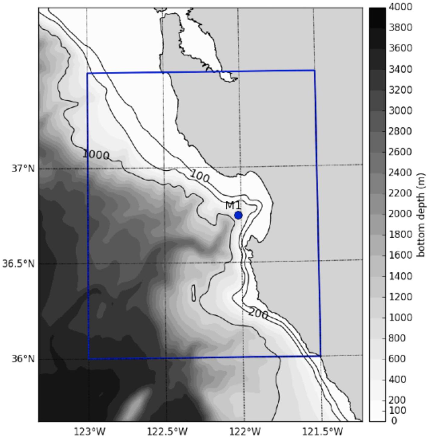
Figure 1. Map of particle release and field sampling location. 10,000 particles were released daily in 2015 from Station M1 (36.747°N, 122.022°W) and tracked for 7 days. Station M1 also represents the location of the field sample. The blue box represents the grid subset used to create the probability map of eDNA origin in Figure 6. The bathymetry represents that of the ROMS model.

Particles were released each day of the year in 2015 until 24 December (358 days) and particle trajectories were tracked for 7 days after they were released. All 10,000 particles were released at the same start time on each day (12:00 GMT) and results were stored at 1-hour time intervals. Particles that hit the coastline before the end of the simulation remained there unless currents transported them back offshore. The choice of coastline action was determined not to affect results (data not shown). Particles that reached the bed were removed from the simulation based on the assumption that eDNA would be incorporated into the bottom sediment upon deposition and is not resuspended.

For this study, we will refer to a “simulation” as a model run that commences on a particular day implemented using a specific value for the settling rate and the decay rate constant. Thus, four simulations were performed per day, resulting in a total of 1432 seven-day simulations: 358 days × 2 settling rate cases × 2 decay rate constant cases.

Analysis of Model Output

Defining Horizontal and Vertical Displacement and Spread

The time evolution of the displacement and spread of the particles was quantified for each simulation. “Displacement” is defined as the displacement of the center of mass (COM) of particles from the release location (Figures 2, 3). “Spread” is defined as the standard deviation of particle distance from the COM (Figures 2, 3). All particles remaining in the water column (i.e., those that did not reach the bottom) were used in the calculations of displacement and spread.

FIGURE 2

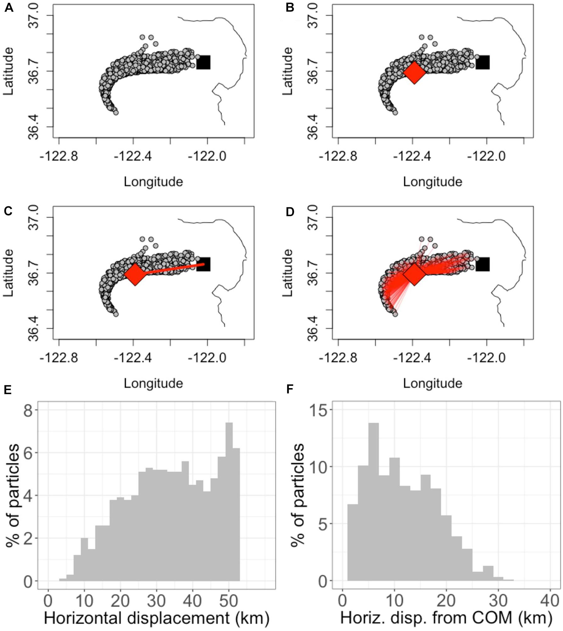
Figure 2. Demonstration of horizontal displacement and spread calculations. The demonstration uses a 1000-particle subset of the 10,000 used in a sample simulation for clarity of visualization. (A) the black square is the point of release, Station M1. The gray circles show the location of particles after being subject to ocean currents for 4 days. (B) the red diamond shows the center of mass (COM) of particles after 4 days. (C) the displacement of the COM from the point of release is shown as a red line. (D) the red lines show the distance from each particle to the COM. (E) A histogram of the displacement of particles from Station M1. (F) A histogram of the displacement of particles from the COM [red lines in Panel (D)] at this point in time (4 days since release). The horizontal displacement metric is defined as the displacement of the COM, which changes in time. The horizontal spread metric is calculated as the standard deviation of particle displacements from the COM, which also changes in time. For this demonstration, at t = 4 days, the horizontal displacement is 33 km and horizontal spread is 6.6 km.

FIGURE 3

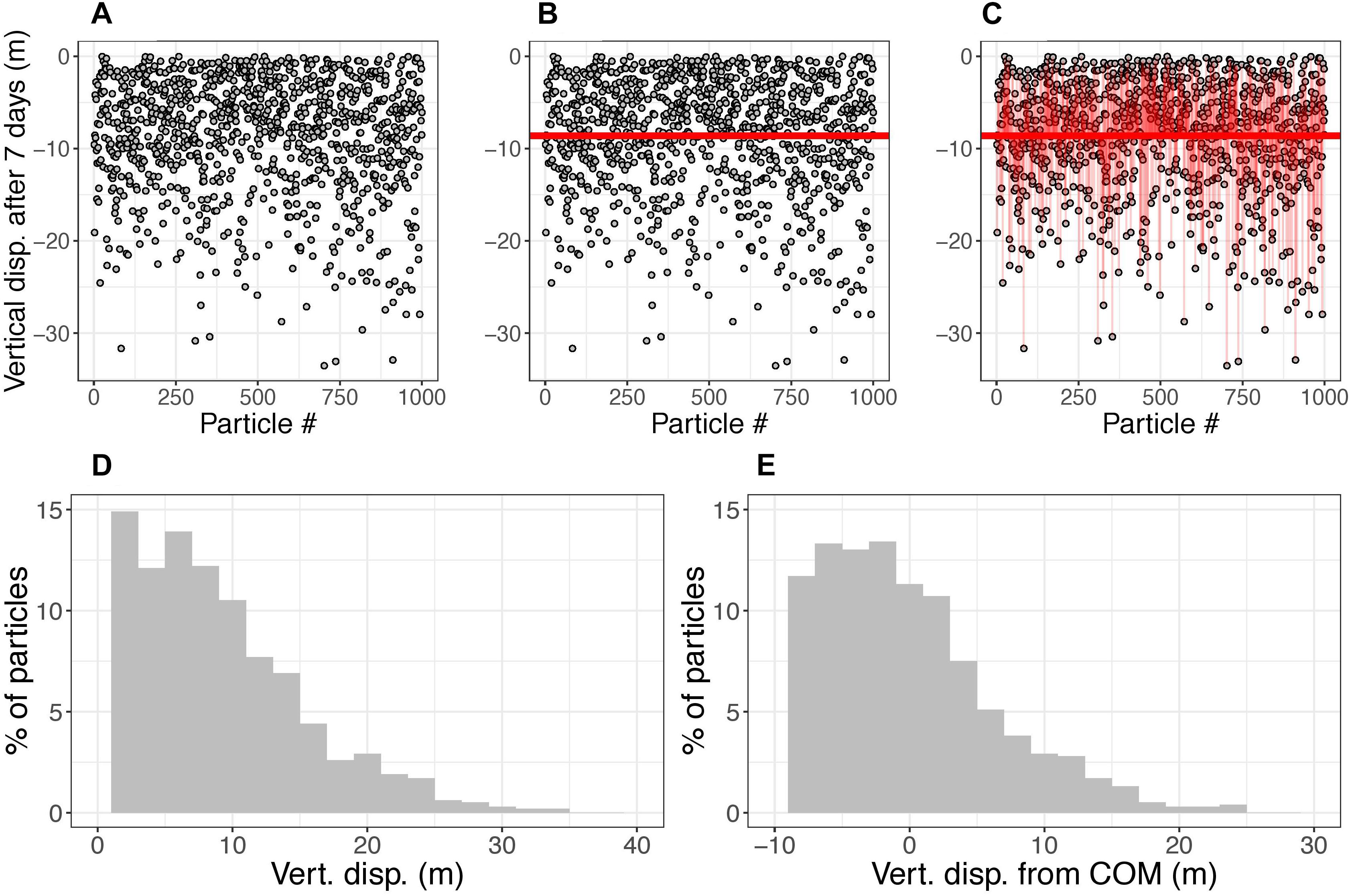
Figure 3. Demonstration of vertical displacement and spread calculations. The demonstration uses a 1000-particle subset of the 10,000 used in a sample simulation. (A) The gray circles show the location of particles (released from surface) after being subject to ocean currents for 7 days. (B) The horizontal line shows the vertical center of mass (COM) of particles after 7 days. Panel (C) the thin vertical red lines show the distance from each particle to the COM. (D,E) histograms of displacement of particles and displacement of particles from the COM, respectively, of the 1000 particles in this simulation at 7 days. The vertical displacement metric is defined as the displacement of the COM, which changes in time. The vertical spread metric is calculated as the standard deviation of particle displacements, which also changes in time. For plotting results, the positive and negative spread are separated. For the statistical models, the spread is calculated as one standard deviation accounting for both the positive and negative variances. For this demonstration, at t = 7 days, the vertical displacement is –8.6 m and spread is 2.4 m in the negative direction, 5.1 m in the positive direction, and 3.9 m considering both directions.

The location of the COM in the horizontal plane was determined by averaging the latitude and longitude of particle locations accounting for the sphericity of the earth (Figure 2B). The horizontal displacement of the COM was calculated by taking the Haversine distance between the latitude and longitude of the COM and the release location (Station M1) (Figure 2C). To determine horizontal spread, the standard deviation of particle displacement from the COM was calculated (Figure 2D).

The COM in the vertical dimension was defined as the average depth of particles. The displacement of the COM was measured as the depth of the COM because particles were released at surface (Figure 3B). For the spread in the vertical direction, the standard deviation of particle displacement was calculated (Figure 3C).

Evaluating the Effect of Settling Rate and Thermocline Depth on eDNA Fate and Transport

To visualize the effect of settling rate on displacement and spread of eDNA over time, results from all simulations were combined and displacement and spread were plotted as a function of time since release for the case of no decay (k = 0 h^–1). The horizontal spread was symmetric, whereas the vertical spread was separated into positive and negative spread after determining by visual assessment that it was skewed (Figures 3C,E and Supplementary Figures S1B,C).

In addition, statistical models were used to investigate associations between several independent variables and displacement and spread using simulations where k = 0 h^–1. Here, the vertical spread was represented using as a single value: the standard deviation of the absolute value of both positive and negative spread. Each model including the following independent variables: thermocline depth (continuous variable: absolute value of thermocline depth on day of particle release at Station M1), settling rate (binary variable: 0 for 0 cm s^–1, 1 for 0.1 cm s^–1), and time (continuous variable: hour since particle release). The thermocline depth was defined as the depth of the 12°C isotherm at Station M1; it was determined for each day of the year by finding the shallowest depth where the ROMS temperature was 12^oC after interpolating between vertical grid cells (Supplementary Figure S2) (Carr et al., 2008; Fiedler, 2010). The models were implemented in R using the “lm” function (R Core Team, 2017) using the following equation:

$$Y=\mathrm{\alpha }+{\mathrm{\beta }}_{\text{TD}}\times TD+{\mathrm{\beta }}_{\text{SR}}\times SR+{\mathrm{\beta }}_{\text{T}}\times t(2)$$

where Y is the dependent variable (horizontal displacement, horizontal spread, vertical displacement, or vertical spread), α is the intercept, β_TD is the coefficient for thermocline depth (TD), β_SR is the coefficient for settling rate (SR), and β_t is the coefficient for time, or hour since release (t). We consider positive and negative coefficients in the model to have a positive or negative association, respectively. A cut-off p-value of 1% was used to test for significant association.

An Analysis Framework Based on Time Scale Ratios

Five non-dimensional numbers can be constructed by comparing the time scales of the six fate and transport processes: (1) vertical advection, (2) vertical settling, (3) horizontal dispersion, (4) vertical dispersion, (5) decay, and (6) horizontal advection. By examining ratios of these time scales, we are able to determine which processes are dominant, and under which conditions. The numbers were formulated to be compared to the time scale of horizontal advection based on the hypothesis that horizontal advection would be the dominant process.

Characteristic parameter values were used to calculate the non-dimensional numbers: L_H0 is a characteristic length scale in the horizontal direction [m], L_V0 is a characteristic length scale in the vertical direction [m], U₀ is a characteristic advective velocity in the horizontal direction [m s^–1], W₀ is a characteristic advective velocity in the vertical direction [m s^–1], κ_H0 is a characteristic horizontal dispersion coefficient [m² s^–1], κ_V0 is a characteristic vertical turbulent diffusivity [m² s^–1], w_s0 is a characteristic settling rate [m s^–1], and k₀ is a characteristic decay rate constant [s^–1]. We combined these characteristic scales into five time scale ratios: $\frac{{\text{W}}_0{\text{L}}_{\text{H}0}}{{\text{U}}_0{\text{L}}_{\text{V}0}}$ (advection scale ratio), $\frac{{\text{w}}_{\text{s}0}{\text{L}}_{\text{H}0}}{{\text{U}}_0{\text{L}}_{\text{V}0}}$ (non-dimensional settling rate), $\frac{{\text{U}}_0{\text{L}}_{\text{H}0}}{{\mathrm{\kappa }}_{\mathrm{H0}}}$ (horizontal Péclet number), $\frac{{\mathrm{\kappa }}_{\mathrm{V0}}{\text{L}}_{\text{H}0}}{{\text{U}}_0{\text{L}}_{\text{V}0}^2}$ (vertical turbulent Péclet number), and $\frac{{\text{k}}_0{\text{L}}_{\text{H}0}}{{\text{U}}_0}$ (effective Damköhler number).

The advection scale ratio compares the time scale of horizontal advection to the time scale of vertical advection. A large value of the advection scale ratio indicates that the time scale of horizontal advection is much larger than the time scale of vertical advection. Conceptually, a large advection scale ratio indicates it takes longer for eDNA to be transported the characteristic length scale in the horizontal (L_H0) by advection than it does for eDNA to be transported the characteristic length scale in the vertical direction (L_V0) by advection. Similarly, the non-dimensional settling rate, the vertical turbulent Péclet number, and the effective Damköhler number compare the time scales of horizontal advection to the time scales of settling, vertical dispersion, and decay, respectively. These numbers can be interpreted in the same manner as the advection scale ratio: large numbers indicate that the corresponding process dominates horizontal advection while small values indicate that horizontal advection dominates. The horizontal Péclet number compares the time scales of horizontal dispersion to horizontal advection and thus the interpretation is reversed. For the Péclet number interpretation, a large value indicates that horizontal advection dominates horizontal dispersion and a small value indicates that dispersion dominates advection.

When calculating the non-dimensional numbers, L_H0 and L_V0 were held constant, w_s0 and k₀ were changed based on the simulation (0 or 0.1 cm s^–1; 0 or 0.055 h^–1, respectively), and U₀, W₀, κ_V0, andκ_H0 varied depending on the date the simulation was initiated. The length scale L_H0 = 5 km was chosen in accordance with the average displacement of eDNA during the course of 1 day (as described in section “Results”) and the length scale L_V0 = 100 m was chosen based on the order of magnitude depth of the thermocline (Supplementary Figure S2). The average of the absolute value of the horizontal and upward sea water velocities over the first day of the simulation from the ROMS model was used for U₀ and W₀, respectively. The depth-integrated average vertical turbulent diffusivity over the first day of the simulation was used for κ_V0 and a depth-integrated κ_H0 was calculated by determining the slope of the variance of particle displacements from the OpenDrift simulations over time for the first day of the 7-day simulation (Liang et al., 2018).

Interpretation of Field Measurements Using the Model

Quantifying eDNA Concentrations From Field Samples

Northern anchovy (Engraulis mordax) eDNA was quantified from field samples (3 biological replicates) collected at Station M1 from 40 m deep on 29 September 2015. The field collection and DNA extraction methods are reported in Andruszkiewicz et al. (2017a); triplicate 1-liter water samples were vacuum filtered onto 0.22 μm pore size Durapore polyvinylidene fluoride filters (Millipore, Burlington, MA, United States) and stored at −80^oC until extracting DNA using the DNeasy Blood and Tissue Kit (Qiagen, Germantown, MD, United States) with minor modifications. The DNA extracts were used to perform quantitative PCR (qPCR) to detect E. mordax eDNA. A published qPCR assay for E. mordax was applied that targets the control region d-loop gene (Sassoubre et al., 2016). The primer/probe sequences were: F 5′ TTCACTTGGCATTTGACGGG 3’, R 5′ TGCTCCTGAGATCACTTATGC 3′, P 5′-FAM- AGGTTGAACATTTTCCTTGCTTGCGA-BHQ. Each DNA extract was amplified in the following 20 μL reaction: Taqman Universal Mastermix II (1×), 0.2 mg ml^–1 bovine serum album (BSA), forward and reverse primer (0.2 μM), probe (0.15 μM), 2 μL of DNA extract, and molecular-biology-grade water (Sigma-Aldrich, St. Louis, MO, United States). Cycle temperature parameters are given in Sassoubre et al. (2016); the initial step is 95°C for 10 min, followed by 40 cycles of 95°C for 15 s and 60°C for 1 min. The cycle quantification (Ct) threshold was set to 0.01. The PCR plate contained triplicate reactions for each of the biological triplicate water samples for a total of 9 reactions of the field sample. The plate also included 3 no template controls with molecular grade water added to the reaction in lieu of DNA extract.

Standards were constructed from DNA extracted from E. mordax tissue using the Qiagen DNeasy Blood and Tissue Kit (Qiagen, Valencia, CA, United States). Extracted DNA was quantified using a QUBIT fluorometer 2.0 (Life Technologies, Grand Island, NY, United States). Standards were run in triplicate along with samples in each PCR plate at the following concentrations: 200 pg per reaction, 20 pg per reaction, 2 pg per reaction, 0.2 pg per reaction, and 0.02 pg per reaction. Standard curve data were pooled and used together to create a regression of DNA concentration per reaction versus Ct to calculate concentrations of unknown samples. The concentrations of unknowns were converted from mass DNA per reaction to mass DNA per volume of water filtered (1 L) using dimensional analysis. The limit of quantification was set at the lowest concentration of a known standard that all three triplicates were consistently assigned a Ct value.

Probability Density Function Map of eDNA Origin

The particle tracking model was used to determine possible locations where eDNA might have been shed from anchovies given the concentration of anchovy eDNA that was measured at Station M1. Particles were released from grid cells within a subset of the model domain every hour prior to the time that the field sample was collected. Particles that passed through Station M1 at the time of field sampling (22:30 GMT on 29 September 2015) within 10 m above or below the sampling depth (40 m) were identified and their origins noted to infer and map possible eDNA origins.

Two maps were created by releasing particles as a single point release every hour for 50 and 91 h prior to sampling. These two times were chosen to match the expected duration of time that eDNA is expected to persist in the environment given the concentration we measured in the field sample (C), an assumed initial concentration of eDNA (C₀), and an assumed decay rate constant k (either 0.1 or 0.055 h^–1 representing high and moderate values from the literature (Thomsen et al., 2012; Sassoubre et al., 2016; Andruszkiewicz et al., 2017a)). There are currently no estimates of how much eDNA is shed by a school of anchovy in the ocean to use for C₀. We assumed an upper bound estimate for C₀ of 1 pg ml^–1 based on the steady-state concentration of anchovy eDNA measured in a mesocosm study, which contained 43 anchovies in an approximately 5000 L tank (Sassoubre et al., 2016). 50 h and 91 h are the times at which C₀ decays to the measured concentration C given the two k values, respectively.

The subset of the ROMS domain to release particles was chosen after running a backtracking method (results not shown) to identify 1405 likely origin grid cells; 10,677 extra grid cells were added surrounding those cells in order to make the subset 136 × 136 grid cells (each grid cell was approximately 1 × 1 km). The resultant subset was bounded by 36.0°N, 123.0°W and 37.5°N, 121.5^oW (Figure 1, blue box) and included 12,082 cells after excluding cells within those bounds that were on land. 100 particles were released from the middle of each grid cell every hour; all particles were released at the surface and were not assigned a settling rate.

After the hourly simulations, the locations of the 1,208,200 particles at 29 September 2015 22:30 GMT (the time of sampling) were evaluated to identify which particles were within the grid cell corresponding to Station M1 (bounded by 36.75°N, 122.027°W and 36.738°N, 122.016^oW) and were between 30 and 50 m deep. If a particle was in the M1 grid cell and sampling depth window, the particle’s starting grid cell was recorded as a possible origin location. The number of particles starting in each grid cell was normalized by the total number of particles that ended in the M1 grid cell to a create probability map. Thus, each cell was assigned a probability that it was the origin cell of eDNA shed assuming either a moderate or fast decay rate constant; the sum of probabilities of all cells for each map was 1.

Results

Time Evolution of eDNA Displacement and Spread

An initial case was examined in which there was no decay of eDNA to understand how far, in the 7-day time limit, it may be transported from its source and to investigate the effect of settling rate on displacement and spread (Figure 4). In the horizontal direction, the center of mass of eDNA was both displaced and spread approximately 30 km after 7 days when there is no settling (Figure 4A). However, horizontal displacement of the center of mass of the eDNA, and the spread, were both approximately 10 km after 7 days with settling (Figure 4B). Inclusion of settling rate decreased horizontal displacement by a factor of three.

FIGURE 4

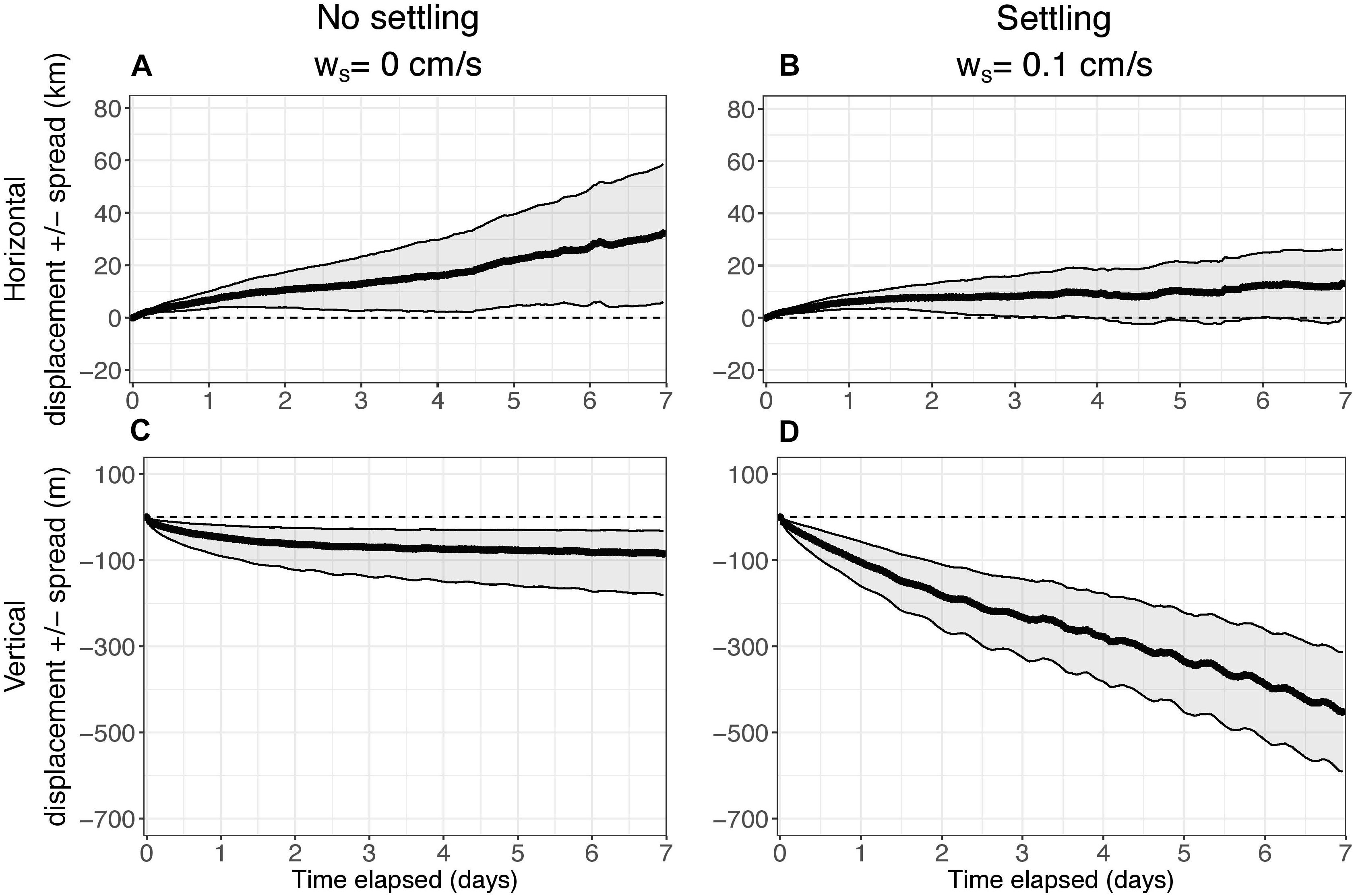
Figure 4. Median horizontal displacement (km) and vertical displacement (m) of the center of mass (COM) of particles as a function of time elapsed over the 7-day simulations for k = 0 h^–1 (no decay). (A,C) show results without settling (w_s = 0 cm s^–1). (B,D) show results with settling (w_s = 0.1 cm s^–1). The edges of the shading represent the median spread (km for horizontal, m for vertical) of particles around the COM. The horizontal spread is symmetric. The vertical spread was slightly skewed, so it was calculated separately for positive and negative directions.

In the vertical direction, the center of mass of eDNA was displaced approximately 100 m and the spread was approximately 50–100 m after 7 days when there is no settling (Figure 4C). However, as expected, with settling, the vertical displacement and spread of eDNA increased; displacement of the center of mass was approximately 500 m and the spread increased to approximately 100–125 m (Figure 4D). The inclusion of settling increased vertical displacement by a factor of about five. For both cases, the vertical spread was greater in the negative direction than the positive direction (Figures 4C,D).

In most simulations, a fraction of the 10,000 particles reached the bottom of the water column before the end of the 7-day simulation (Supplementary Figure S3). This occurred more frequently when particles when settling was included in the simulations (median: 9629; minimum: 680; maximum: 9997) (Supplementary Figure S3B). Without settling, the median number of particles that reached the bottom after 7 days was less than 5000 (half the total number of particles released) (median: 4352; minimum: 2, maximum: 8615) (Supplementary Figure S3A). However, with settling, after approximately 3 days, the median number of particles reaching the bottom exceeded 5000 (Supplementary Figure S3B).

Statistical models explored how displacement and spread covaried with the thermocline depth on the day of particle release, settling rate, and hour since release. The quantity “hour-since-release” was statistically significant and positively associated (i.e., coefficients in Eq. 2 were positive and had a p-value of <0.01) with horizontal displacement and spread (Table 1 and Supplementary Tables S1, S2). Thermocline depth and settling rate were statistically significant and negatively associated with both horizontal displacement and spread. The association with settling rate is consistent with the results in Figure 4 illustrating that the distribution of eDNA is both displaced and spread less when it is assigned a settling rate (Table 1 and Supplementary Tables S1, S2). The model for horizontal displacement explained 28% of its variability [displacement (r² = 0.284)], while the model for horizontal spread explained 46% of its variability (spread r² = 0.462).

TABLE 1

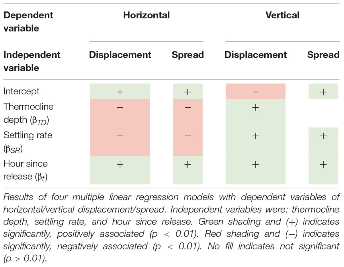
Table 1. Summary of statistical models.

Vertical displacement was significantly positively associated with thermocline depth, settling rate, and hour-since-release (Table 1 and Supplementary Tables S1, S2). These results indicate that as the thermocline became deeper, as time progressed, or when a settling rate was included, the distribution of eDNA was displaced farther in the vertical direction. Vertical spread was not significantly associated with thermocline depth but was significantly positively associated with settling rate and hour since release (Table 1 and Supplementary Tables S1, S2). Both vertical models were able to explain more that 65% of the independent variables’ variability (displacement r² = 0.682; spread r² = 0.669).

Dominant Transport Processes

Figure 5 shows histograms for three of the five non-dimensional numbers: the non-dimensional settling rate (comparing the time scale of horizontal advection to settling; Figure 5A), the Péclet number (comparing the time scale of horizontal dispersion to horizontal advection; Figure 5B), and the effective Damköhler number (comparing the time scale of horizontal advection to decay; Figure 5C). The other two non-dimensional numbers comparing time scales of horizontal advection to vertical advection (the advection scale ratio) and horizontal advection to vertical mixing (vertical turbulent Péclet number) had values much smaller than 1 for all simulations (data not shown), indicating that vertical advection and mixing were not dominant relative to horizontal advection in any of the simulations.

FIGURE 5

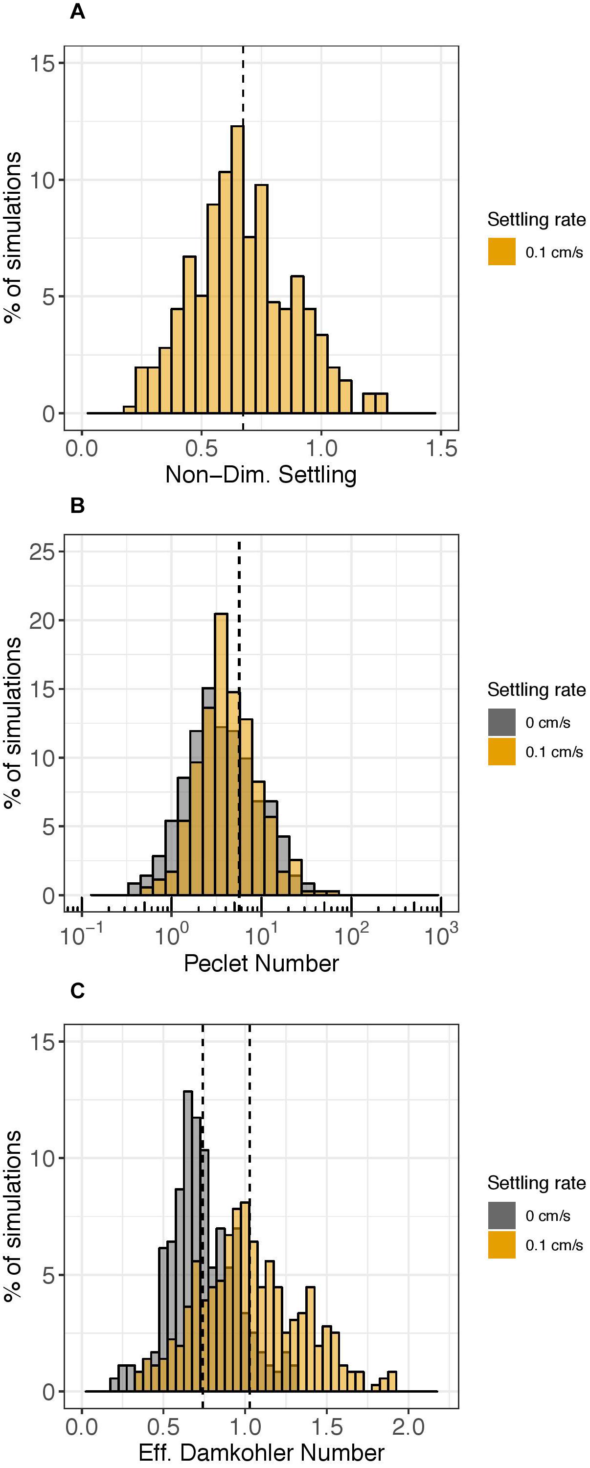
Figure 5. Histograms of select non-dimensional numbers. The y-axis represents the percent of simulations over the year (n = 358 for each settling rate case) that had the corresponding value on the x-axis after 1 day of the particle tracking simulation. Gray shading represents simulations without settling (w_s = 0 cm s^–1) and orange shading represents simulations with settling (w_s = 0.1 cm s^–1). The non-dimensional settling rate is plotted in Panel (A). The Pèclet number (log-scale) is shown in Panel (B) and the effective Damköhler number is shown in Panel (C). Vertical dashed lines show mean values; in Panel (B), the two vertical lines overlap.

The non-dimensional settling rate, which compares the time scale of horizontal advection to settling, was greater than 1 for only 25 of the 358 days simulated (about 7%) (Figure 5A). Physically, this means that when the time scale ratio of horizontal advection to settling was greater than 1, eDNA was transported 100 m vertically (L_V0) by settling (w_s0) faster than it was transported 5 km horizontally (L_H0) by advection (U₀).

The Péclet number comparing the time scale of horizontal dispersion to horizontal advection was consistently larger than 1 and varied by 2 orders of magnitude over the course of the year (Figure 5B). Thus, although horizontal advection generally dominated horizontal dispersion, for certain simulations, the processes had nearly equal influence. The very small effect of settling on the Péclet number can be seen in Figure 5 and was not significant; the null hypothesis that the difference in median Péclet number with or without settling is zero was not rejected (Figure 5B, orange vs. gray; Wilcox signed rank test, p = 0.04).

The ratio of time scales of horizontal advection to decay, represented by the effective Damköhler number, oscillated around 1 (Figure 5C). The value for the characteristic decay rate constant used for calculating the effective Damköhler number was 0.055 h^–1; hence the time scale of decay was approximately 18 h (1/0.055 h^–1). Thus, the effective Damköhler number indicates whether the time required for eDNA to be transported 5 km (L_H0) by horizontal advection (U₀) is greater than or less than 18 h. 30% of simulations had an effective Damköhler number with a value greater than 1, with a higher percentage when a settling rate was assigned (48%) compared to when a settling rate was not assigned (11%) (Figure 5C, orange vs. gray). The mean effective Damköhler number with settling was 1.0 compared to 0.74 without settling (Figure 5C, dashed vertical lines; Wilcox signed rank test p < 0.01) and the null hypothesis that the median difference in effective Damköhler number with or without settling was zero was rejected.

Application to Field Samples

The E. mordax qPCR assay had an efficiency of 94% and a limit of detection (lowest standard that at least one of triplicates was assigned a Ct value) of 0.01 pg μL^–1 of DNA extract. The extraction blank, filter blank, and no template controls had undetermined Ct values, indicating no contamination. The three biological replicates collected at 40 m depth at station M1 had an average concentration of 0.065 pg μL^–1, which, by dimensional analysis and after converting from volume of extract amplified to volume of water filtered, corresponds to 6.5 pg of anchovy eDNA per L of water. This concentration represents C and can be used in a first order decay model with C₀ [1 pg per mL of water based on Sassoubre et al. (2016)] and the two k values for moderate and fast decay (0.055 h^–1 and 0.1 h^–1) to obtain the times of 50 and 91 h, respectively, at which eDNA was likely shed from a school of anchovies in the past based on the field sample concentration.

The probability maps demonstrated that the origin of anchovy eDNA could have been located up to approximately 40 km away and that it was likely shed south of Station M1 (Figure 6). A larger value for the decay rate constant limits the possible locations of origin as time subject to ocean currents is reduced. Under the scenario of fast decay, it is most likely that eDNA originated within 20 km of Station M1 (Figure 6A). The cumulative probability that eDNA originated from within 20 km of Station M1 was 80% assuming a moderate decay rate constant (0.055 h^–1) compared to 96% assuming a fast decay rate constant (0.1 h^–1) (Figure 6B vs. Figure 6A).

FIGURE 6

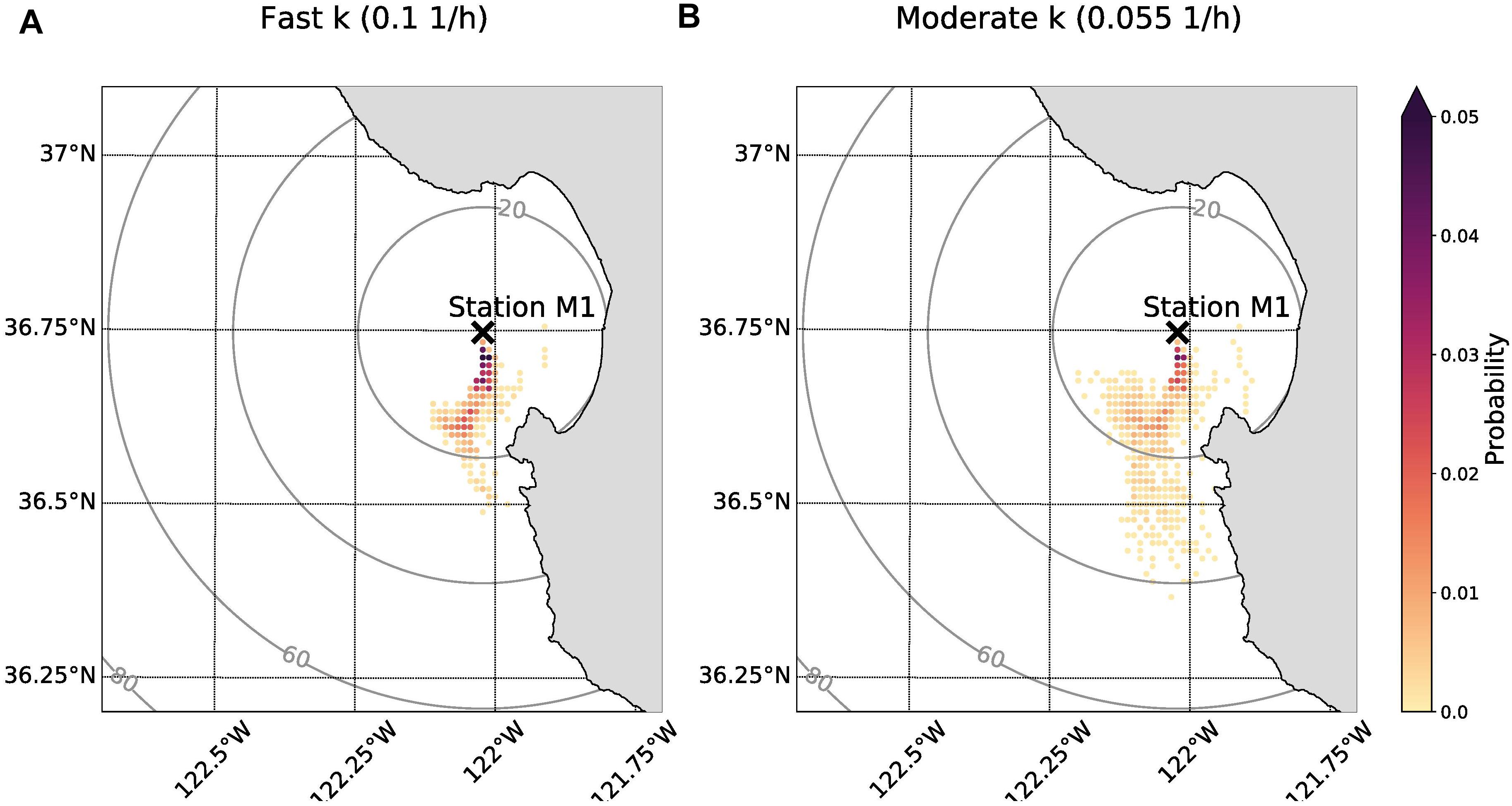
Figure 6. Probability maps showing anchovy eDNA origin given field sample detection on 29 September 2015. The sampling location (Station M1) is indicated with black “X.” The color corresponds to the probability that eDNA originated in that cell. The rings indicate distance from Station M1 in units of km. (A) Origin location probabilities of eDNA if the decay rate constant was fast (0.1 h^–1). (B) Origin location probabilities of eDNA if the decay rate constant was moderate (0.055 h^–1). The sum of all probabilities for each panel is equal to 1.

Discussion

Settling Affects Horizontal and Vertical Displacement

Settling of eDNA strongly impacted eDNA displacement and spread. The center of mass of neutrally buoyant eDNA was displaced less and spread less in the vertical direction than eDNA that was assigned a settling rate. In the horizontal, the center of mass of neutrally buoyant eDNA was displaced more and spread farther than settling eDNA, a result possibly attributable to depth variation in horizontal currents: when eDNA is assigned a settling rate, it may be subject to weaker horizontal currents. Surface currents are estimated to be approximately twice the magnitude of currents at intermediate depths (i.e., 25–150 m) in MB (Breaker and Broenkow, 1994).

The results of eDNA vertical spread provide estimates of how sampling depth might relate to shedding depth by providing a length scale to compare to sampling depth. For example, the positive vertical spread of neutrally buoyant eDNA was approximately 50 m after 7 days. This implies that eDNA is not likely to be mixed upward greater than 50 m in 7 days. Thus, the depth at which eDNA was shed from an organism is not likely greater than 50 m deeper than the sampling depth, assuming the eDNA was neutrally buoyant. Furthermore, the vertical mixing time scale can also be used to bound horizontal displacement. These time scale and length scale comparisons can be manipulated to provide estimates of maximum eDNA displacement.

The simulations in this paper were performed assuming an estimated settling rate value from research on marine snow (upper-end of published values) because there are currently no estimates of eDNA settling rates in the ocean. The different patterns of horizontal and vertical displacement and spread, the results of the statistical models, and the values of the non-dimensional setting rate all suggest that settling is an important process controlling the fate and transport of eDNA. The time scale of settling would always dominate the time scale of horizontal advection (i.e., the non-dimensional settling rate >1) if the settling rate were greater than 0.47 cm s^–1, which is unrealistically high. On the other hand, in order for the time scale of horizontal advection to always be greater than the time scale of settling, the settling rate would need to be less than 0.08 cm s^–1. In reality, settling rates are likely to be within this range and due to the variety of forms of eDNA, the influence of settling will be important in eDNA transport. Clearly, research is needed to document eDNA settling rates.

Decay Limits eDNA Transport Distances

The spatial extent of eDNA transport from its origin is controlled, in part, by the persistence of eDNA in the water column. We performed simulations over 7 days and found that when using a moderate decay rate constant (0.055 h^–1), eDNA decayed in 30% of the simulations before it was transported 5 km in the horizontal direction (effective Damköhler number >1). Hence, eDNA decay must be considered when estimating transport distances.

It is important to note that if a lower bound on k (0.01 h^–1) was used in calculating the effective Damköhler number, the ratio of decay to horizontal advection time scales would always be less than 1 (i.e., eDNA would always be transported 5 km or farther) and if an upper bound (0.1 h^–1) were used, the ratio of decay to horizontal advection time scales would be greater than 1 in 89% of simulations (i.e., only 11% of eDNA shed would be transported further than 5 km). This simple exercise demonstrates the need for more information about decay rate constants in order to impose a spatial bound on eDNA origin. For eDNA to consistently decay faster than it can be advected 5 km (effective Damköhler number >1), the decay rate constant would need to be 0.26 h^–1 and for eDNA to always be advected more than 5 km before decaying (effective Damköhler number always <1), the decay rate constant would need to be less than 0.029 h^–1. Reported range of decay rate constants in marine water ranges from 0.0097 to 0.1 h^–1 (Collins et al., 2018). These results can provide researchers conducting field studies with estimates of transport distances if a decay rate constant is known a priori by computing this time scale ratio.

Thermocline Depth Is Associated With Horizontal and Vertical Displacement

The results of the statistical models demonstrate that thermocline depth was significantly associated with the eDNA transport. A shallower thermocline depth resulted in greater horizontal displacement and spread and decreased vertical displacement. The thermocline depth was used as a proxy for upwelling conditions (Breaker and Broenkow, 1994). Therefore, the results suggest that in MB, upwelling conditions give rise to greater horizontal eDNA transport and decreased vertical displacement.

The finding that displacement and spread are affected by thermocline depth may be useful for interpreting eDNA results from field samples. If eDNA sampling in MB occurs during upwelling conditions, horizontal displacement and spread are expected to be greater than during non-upwelling conditions. Therefore, the distributions of potential origin locations of eDNA collected in a field sample during upwelling are likely to broader than the extent of potential origin locations of eDNA collected in a water sample during non-upwelling conditions. Similarly, if water sampling occurs during an upwelling event, the range of depths from which eDNA could have originated compared to the sampling depth will likely be narrower than if sampling occurred in the absence of upwelling due to the decreased vertical displacement.

Modeling Provides Spatial Bounds of eDNA Origin From Field Samples

We illustrated how modeling can provide probability maps indicating origin locations of eDNA. The modeling framework is set up such that a variety of assumptions can be made to visualize probabilities for different ecological situations. For example, we assumed that the anchovy eDNA came from a single location. In reality, the concentration of anchovy eDNA found in a field sample could have contributions from multiple sources at multiple points in time. Particle releases can be customized to create a variety of scenarios to explore different possibilities. Additionally, we had to assume an initial concentration of eDNA (C₀). There is currently very little information available to infer C₀ values in the field.

We chose to model eDNA in the field study as neutrally buoyant because there are currently no reliable estimates of eDNA settling rates in the literature. Furthermore, although we collected eDNA from the water using a 0.22 μm-pore size filter, it is difficult to assess the size of the captured eDNA because particles smaller than 0.22 μm in diameter, as well as dissolved eDNA, can also be captured via electrostatic and hydrophobic interactions between the eDNA and the filter (Hickel, 1984). Additionally, the shape (including the fractal dimension), and density of the eDNA would be needed to estimate a settling rate (Boehm and Grant, 2001). Finally, there is uncertainty about the form and size fractionation of eDNA (Takahara et al., 2012; Turner et al., 2014; Eichmiller et al., 2015; Sassoubre et al., 2016). When there is a better understanding of eDNA form and properties, model parameters may be improved.

Limitations and Future Research

This framework has been built with an ongoing goal of improvement. In particular, without published estimates of settling rates of eDNA in the environment, we had to resort to using an upper-end value determined for marine snow. We, therefore, strongly suggest that researchers quantify settling rates of eDNA. We also assumed a constant decay rate in our simulations, even though eDNA decay in ocean water may be more appropriately modeled using more than one decay rate because of variation in environmental stressors. Furthermore, decay might not be a simple first-order process as it is assumed in this, and many other, studies (e.g., Sassoubre et al., 2016; Andruszkiewicz et al., 2017a). Future work should investigate other decay models including models with a shoulder or an inactivation time lag. Finally, all particles were released at the surface of the water column, but it is more realistic that organisms shed eDNA at different depths in the water column. We released particles at depths of 100 m (data not shown) and found a small yet significant effect of release depth on transport, suggesting that additional work should investigate how release depth affects eDNA fate and transport.

Using numerical ocean models with Lagrangian particle tracking improves our current understanding of eDNA transport in the coastal ocean. This work provides baselines for visualizing the spatial extent to which eDNA can be transported given best available estimates of eDNA persistence. We provide the first approximations of the displacement and spread of eDNA distributions in the coastal ocean assuming a single point release, and the first probability map of eDNA origin based on a field sample. The majority of studies investigating eDNA in the ocean focus on concentrations of eDNA found in water samples, but these studies do not report approximate ranges of origin. For many research questions that could be answered using eDNA assays, having confidence in the spatial bounds of the source of the eDNA sampled would be extremely useful. The relative ease and low computational cost of particle tracking simulations make this method approachable and applicable and will enable managers and researchers to better understand the context in which they are interpreting eDNA field sample results.

Data Availability

The datasets generated for this study are available on request to the corresponding author.

Author Contributions

EA designed and performed the study, analyzed the results, and wrote the manuscript. JK, OF, and NO helped to design the study, analyze the results, and reviewed the manuscript. AL and CE provided the ROMS model, helped to analyze the results, and reviewed the manuscript. AB designed the study, analyzed the results, and wrote and reviewed the manuscript.

Funding

EA received funding from the Charles H. Leavell Graduate Student Fellowship and the EPA STAR program under STAR Fellowship Assistance Agreement no. F15E211913419 awarded by the United States Environmental Protection Agency (EPA). The publication has not been formally reviewed by EPA. The views expressed in this publication are solely those of EA and co-authors, and EPA does not endorse any products or commercial services mentioned in this publication.

Conflict of Interest Statement

The authors declare that the research was conducted in the absence of any commercial or financial relationships that could be construed as a potential conflict of interest.

Acknowledgments

Some of the computing for this project was performed on the Sherlock cluster. We acknowledged Stanford University and the Stanford Research Computing Center for providing computational resources and support through the use of the Sherlock cluster that contributed to these research results.

Supplementary Material

The Supplementary Material for this article can be found online at: https://www.frontiersin.org/articles/10.3389/fmars.2019.00477/full#supplementary-material

FIGURE S1 | Sensitivity of particle tracking releases to number of particles released. Panel (A) shows the mean squared horizontal displacement from the center of mass (COM) (km²) over time since release of particles. Panel (B) shows the mean squared vertical displacement from the COM in the positive direction (m²) over time and Panel (C) shows the mean squared vertical displacement from the COM in the negative direction (m²) over time. Colors of markers correspond to the number of particles released: 10 (red), 100 (orange), 1,000 (green), 10,000 (black), and 100,000 (blue).

FIGURE S2 | Thermocline depth, as defined by 12°C isotherm, from the ROMS model for 2015 at Station M1.

FIGURE S3 | Number of particles reaching bottom over the course of the simulation. Panel (A) includes simulations where no settling rate is applied, and Panel (B) shows simulations when a settling rate of 0.1 cm s⁻¹ is applied. The solid lines show the median number of particles reaching the bottom over the course of the year. The edge of the shading shows the 25th and 75th percentile and the dashed lines show the minimum and maximums.

TABLE S1 | Coefficients of linear model for horizontal and vertical displacement and spread. Bold indicates 1% significance.

TABLE S2 | Performance of linear models. Bold indicates 1% significance.

References

Akatsuka, M., Takayama, Y., and Ito, K. (2018). “Applicability of environmental DNA analysis and numerical simulation to evaluate seagrass inhabitants in a Bay,” in Proceedings of the 29th International Ocean and Polar Engineering Conference, (Sapporo: International society of offshore and polar engineers), 1538–1544.

Google Scholar

Alldredge, A., and Gotschalk, C. (1988). In situ settling behavior of marine snow. Limnol. Oceanogr. 33, 339–351. doi: 10.1016/j.scitotenv.2016.09.115

PubMed Abstract | CrossRef Full Text | Google Scholar

Andruszkiewicz, E. A., Sassoubre, L. M., and Boehm, A. B. (2017a). Persistence of marine fish environmental DNA and the influence of sunlight. PLoS One 12:e0185043. doi: 10.1371/journal.pone.0185043

PubMed Abstract | CrossRef Full Text | Google Scholar

Andruszkiewicz, E. A., Starks, H. A., Chavez, F. P., Sassoubre, L. M., Block, B. A., and Boehm, A. B. (2017b). Biomonitoring of marine vertebrates in Monterey Bay using eDNA metabarcoding. PLoS One 12:e176343. doi: 10.1371/journal.pone.0176343

PubMed Abstract | CrossRef Full Text | Google Scholar

Antonov, J. I., Locarnini, R. A., Boyer, T. P., Mishonov, A. V., and Garcia, H. E. (2006). “World Ocean atlas 2005,” in NOAA Atlas NESDIS, ed. S. Levitus (Washington, DC: United States Government Publishing Office), 62.

Google Scholar

Block, B. A., Jonsen, I. D., Jorgensen, S. J., Winship, A. J., Shaffer, S. A., Bograd, S. J., et al. (2011). Tracking apex marine predator movements in a dynamic ocean. Nature 475, 86–90. doi: 10.1038/nature10082

PubMed Abstract | CrossRef Full Text | Google Scholar

Boehm, A. B., and Grant, S. B. (2001). A steady state model of particulate organic carbon flux below the mixed layer and application to the joint Global Ocean flux study. J. Geophys. Res. 106, 227–231.

Google Scholar

Breaker, L. C., and Broenkow, W. W. (1994). “The circulation of Monterey Bay and related processes,” in Oceanography and Marine Biology: An Annual Review, eds A. D. Ansell, R. N. Gibson, and M. Barnes (Boca Raton, FL: CRC Press), 1–65.

Google Scholar

Carr, S. D., Capet, X. J., McWilliams, J. C., Pennington, J. T., and Chavez, F. P. (2008). The influence of diel vertical migration on zooplankton transport and recruitment in an upwelling region: estimates from a coupled behavioral-physical model. Fish. Oceanogr. 17, 1–15. doi: 10.1111/j.1365-2419.2007.00447.x

CrossRef Full Text | Google Scholar

Coll, M., Libralato, S., Tudela, S., Palomera, I., and Pranovi, F. (2008). Ecosystem overfishing in the ocean. PLoS One 3:e3881. doi: 10.1371/journal.pone.0003881

PubMed Abstract | CrossRef Full Text | Google Scholar

Collins, R. A., Wangensteen, O. S., O’Gorman, E. J., Mariani, S., Sims, D. W., and Genner, M. J. (2018). Persistence of environmental DNA in marine systems. Commun. Biol. 1:185. doi: 10.1038/s42003-018-0192-6

PubMed Abstract | CrossRef Full Text | Google Scholar

Dagestad, K. F., Röhrs, J., Breivik, Ø, and Ådlandsvik, B. (2017). OpenDrift v1.0: a generic framework for trajectory modeling. Geosci. Model Dev. Discuss. 11, 1–28. doi: 10.5194/gmd-2017-205

CrossRef Full Text | Google Scholar

de Groot, R. S., Alkemade, R., Braat, L., Hein, L., and Willemen, L. (2010). Challenges in integrating the concept of ecosystem services and values in landscape planning, management and decision making. Ecol. Complex 7, 260–272. doi: 10.1016/j.ecocom.2009.10.006

CrossRef Full Text | Google Scholar

Deiner, K., Fronhofer, E. A., Machler, E., Walser, J.-C., and Altermatt, F. (2016). Environmental DNA reveals that rivers are conveyer belts of biodiversity information. Nat. Commun. 7, 1–9. doi: 10.1038/ncomms12544

PubMed Abstract | CrossRef Full Text | Google Scholar

Drake, P. T., Edwards, C. A., and Barth, J. A. (2011). Dispersion and connectivity estimates along the U.S. west coast from a realistic numerical model. J. Mar. Res. 69, 1–37. doi: 10.1357/002224011798147615

CrossRef Full Text | Google Scholar

Drake, P. T., Edwards, C. A., Morgan, S. G., and Dever, E. P. (2013). Influence of larval behavior on transport and population connectivity in a realistic simulation of the California current system. J. Mar. Res. 71, 317–350. doi: 10.1357/002224013808877099

CrossRef Full Text | Google Scholar

Drake, P. T., Edwards, C. A., Morgan, S. G., and Satterthwaite, E. V. (2018). Shoreward swimming boosts modeled nearshore larval supply and pelagic connectivity in a coastal upwelling region. J. Mar. Syst. 187, 96–110. doi: 10.1016/j.jmarsys.2018.07.004

CrossRef Full Text | Google Scholar

Edgar, G. J., Barrett, N. S., and Morton, A. J. (2004). Biases associated with the use of underwater visual census techniques to quantify the density and size-structure of fish populations. J. Exp. Mar. Biol. Ecol. 308, 269–290. doi: 10.1016/j.jembe.2004.03.004

CrossRef Full Text | Google Scholar

Edwards, K. P., Hare, J. A., and Werner, F. E. (2008). Dispersal of black sea bass (Centropristis striata) larvae on the southeast U.S. continental shelf: results of a coupled vertical larval behavior 3D circulation model. Fish. Oceanogr. 17, 299–315. doi: 10.1111/j.1365-2419.2008.00480.x

CrossRef Full Text | Google Scholar

Eichmiller, J. J., Miller, L. M., and Sorensen, P. W. (2015). Optimizing techniques to capture and extract environmental DNA for detection and quantification of fish. Mol. Ecol. Resour. 16, 56–68. doi: 10.1111/1755-0998.12421

PubMed Abstract | CrossRef Full Text | Google Scholar

Fiedler, P. C. (2010). Comparison of objective descriptions of the thermocline. Limnol. Oceanogr. Methods 8, 313–325. doi: 10.4319/lom.2010.8.313

CrossRef Full Text | Google Scholar

Fischer, H., List, E. J., Koh, R. C. Y., Imberger, J., and Brooks, N. H. (1979). Mixing in Inland and Coastal Waters. Cambridge, MA: Academic Press.

Google Scholar

Goldberg, C. S., Turner, C. R., Deiner, K., Klymus, K. E., Thomsen, P. F., Murphy, M. A., et al. (2016). Critical considerations for the application of environmental DNA methods to detect aquatic species. Methods Ecol. Evol. 7, 1299–1307. doi: 10.1111/2041-210X.12595

CrossRef Full Text | Google Scholar

Haigh, R., Ianson, D., Holt, C. A., Neate, H. E., and Edwards, A. M. (2015). Effects of ocean acidification on temperate coastal marine ecosystems and fisheries in the Northeast Pacific. PLoS One 10:e117533. doi: 10.1371/journal.pone.0117533

PubMed Abstract | CrossRef Full Text | Google Scholar

Hattam, C., Atkins, J. P., Beaumont, N. J., Borger, T., Bohnke-Henrichs, A., Burdon, D., et al. (2015). Marine ecosystem services: linking indicators to their classification. Ecol. Indic. 49, 61–75. doi: 10.1016/j.ecolind.2014.09.026

CrossRef Full Text | Google Scholar

Hickel, W. (1984). Seston retention by Whatman G/C glass-fiber filters. Mar. Ecol. Prog. Ser. 16, 185–191. doi: 10.3354/meps016185

CrossRef Full Text | Google Scholar

Hodur, R., Pullen, J., Cummings, J., Martin, P., and Rennick, M. A. (2002). The coupled ocean/atmospheric mesoscale prediction system. Oceanography 15, 88–98. doi: 10.1175/BAMS-D-14-00164.1

PubMed Abstract | CrossRef Full Text | Google Scholar

Hunter, J. R. (1987). “The application of lagrangian particle-tracking techniques to modelling of dispersion in the sea,” in Numerical Modelling: Applications to Marine Systems North-Holland Mathematics Studies, ed. J. Noye (Amsterdam: Elsevier).

Google Scholar

Huret, M., Runge, J. A., Chen, C., Cowles, G., Xu, Q., and Pringle, J. M. (2007). Dispersal modeling of fish early life stages: sensitivity with application to Atlantic cod in the western Gulf of Maine. Mar. Ecol. Prog. Ser. 347, 261–274. doi: 10.3354/meps06983

CrossRef Full Text | Google Scholar

Kelly, R. P., Port, J. A., Yamahara, K. M., and Crowder, L. B. (2014). Using environmental DNA to census marine fishes in a large mesocosm. PLoS One 9:e86175. doi: 10.1371/journal.pone.0086175

PubMed Abstract | CrossRef Full Text | Google Scholar

Lett, C., Verley, P., Mullon, C., Parada, C., Brochier, T., Penven, P., et al. (2008). A lagrangian tool for modelling ichthyoplankton dynamics. Environ. Model. Softw. 23, 1210–1214. doi: 10.1016/j.envsoft.2008.02.005

CrossRef Full Text | Google Scholar

Liang, J.-H., Wan, X., Rose, K. A., Sullivan, P. P., and McWilliams, J. C. (2018). Horizontal dispersion of buoyant materials in the ocean surface boundary layer. J. Phys. Oceanogr. 48, 2103–2125. doi: 10.1175/JPO-D-18-0020.1

CrossRef Full Text | Google Scholar

Locarnini, R. A., Mishonov, A. V., Antonov, J. I., Boyer, T. P., and Garcia, H. E. (2006). “World Ocean altas 2005,” in NOAA Atlas NESDIS, ed. S. Levitus (Washington, DC: United States Government Publishing Office), 61.

Google Scholar

McCauley, D. J., Pinsky, M. L., Palumbi, S. R., Estes, J. A., Joyce, F. H., and Warner, R. R. (2015). Marine defaunation: animal loss in the Global Ocean. Science 347:1255641. doi: 10.1126/science.1255641

PubMed Abstract | CrossRef Full Text | Google Scholar

Miya, M., Sato, Y., Fukunaga, T., Sado, T., Poulsen, J. Y., Sato, K., et al. (2015). MiFish, a set of universal PCR primers for metabarcoding environmental DNA from fishes: detection of more than 230 subtropical marine species. R. Soc. Open Sci. 2:150088. doi: 10.1098/rsos.150088

PubMed Abstract | CrossRef Full Text | Google Scholar

Navas, J. M., Telfer, T. C., and Ross, L. G. (2011). Application of 3D hydrodynamic and particle tracking models for better environmental management of finfish culture. Cont. Shelf Res. 31, 675–684. doi: 10.1016/j.csr.2011.01.001

CrossRef Full Text | Google Scholar

Ogram, A., Sayler, G., and Barkay, T. (1987). The extraction and purification of microbial DNA from sediments. J. Microbiol. Methods 7, 57–66. doi: 10.1016/0167-7012(87)90025-x

CrossRef Full Text | Google Scholar

Port, J. A., O’Donnell, J. L., Romero-Maraccini, O. C., Leary, P. R., Litvin, S. Y., Nickols, K. J., et al. (2015). Assessing vertebrate biodiversity in a kelp forest ecosystem using environmental DNA. Mol. Ecol. 25, 527–541. doi: 10.1111/mec.13481

PubMed Abstract | CrossRef Full Text | Google Scholar

R Core Team (2017). R: A Language and Environment for Statistical Computing. Available at: http://www.R-project.org/ (accessed October 21, 2017).

Google Scholar

Robins, P. E., Neill, S. P., Giménez, L., Jenkins, S. R., and Malham, S. K. (2013). Physical and biological controls on larval dispersal and connectivity in a highly energetic shelf sea. Limnol. Oceanogr. 58, 505–524. doi: 10.4319/lo.2013.58.2.0505

CrossRef Full Text | Google Scholar

Sansom, B. J., and Sassoubre, L. M. (2017). Environmental DNA (eDNA) shedding and decay rates to model freshwater mussel eDNA transport in a river. Environ. Sci. Technol. 51, 14244–14253. doi: 10.1021/acs.est.7b05199

PubMed Abstract | CrossRef Full Text | Google Scholar

Sassoubre, L. M., Yamahara, K. M., Gardner, L. D., Block, B. A., and Boehm, A. B. (2016). Quantification of environmental DNA (eDNA) shedding and decay rates for three marine fish. Environ. Sci. Technol. 50, 10456–10464. doi: 10.1021/acs.est.6b03114

PubMed Abstract | CrossRef Full Text | Google Scholar

Schratzberger, M., Dinmore, T., and Jennings, S. (2002). Impacts of trawling on the diversity, biomass and structure of meiofauna assemblages. Mar. Biol. 140, 83–93. doi: 10.1007/s002270100688

CrossRef Full Text | Google Scholar

Shogren, A. J., Tank, J. L., Andruszkiewicz, E. A., Olds, B. P., Jerde, C. L., and Bolster, D. (2016). Modelling the transport of environmental DNA through a porous substrate using continuous flow-through column experiments. J. R. Soc. Interface 13:20160290. doi: 10.1098/rsif.2016.0290

PubMed Abstract | CrossRef Full Text | Google Scholar

Taberlet, P., Coissac, E., Hajibabaei, M., and Rieseberg, L. H. (2012). Environmental DNA. Mol. Ecol. 21, 1789–1793.

Google Scholar

Takahara, T., Minamoto, T., Yamanaka, H., Doi, H., and Kawabata, Z. (2012). Estimation of fish biomass using environmental DNA. PLoS One 7:e35868. doi: 10.1371/journal.pone.0035868

PubMed Abstract | CrossRef Full Text | Google Scholar

Thomsen, P. F., Kielgast, J., Iversen, L. L., Moller, P. R., Rasmussen, M., and Willerslev, E. (2012). Detection of a diverse marine fish fauna using environmental DNA from seawater samples. PLoS One 7:e41732. doi: 10.1371/journal.pone.0041732

PubMed Abstract | CrossRef Full Text | Google Scholar

Thomsen, P. F., Moller, P. R., Sigsgaard, E. E., Knudsen, S. W., Jorgensen, O. A., and Willerslev, E. (2016). Environmental DNA from seawater samples correlate with trawl catches of subarctic, deepwater fishes. PLoS One 11:e165252. doi: 10.1371/journal.pone.0165252

PubMed Abstract | CrossRef Full Text | Google Scholar

Thomsen, P. F., and Willerslev, E. (2015). Environmental DNA: an emerging tool in conservation for monitoring past and present biodiversity. Biol. Conserv. 183, 4–18. doi: 10.1016/j.biocon.2014.11.019

CrossRef Full Text | Google Scholar

Thygesen, U. H. (2011). How to reverse time in stochastic particle tracking models. J. Mar. Syst. 88, 159–168. doi: 10.1016/j.jmarsys.2011.03.009

PubMed Abstract | CrossRef Full Text | Google Scholar

Turner, C. R., Barnes, M. A., Xu, C. C. Y., Jones, S. E., Jerde, C. L., and Lodge, D. M. (2014). Particle size distribution and optimal capture of aqueous macrobial eDNA. Methods Ecol. Evol. 5, 676–684. doi: 10.1111/2041-210X.12206

CrossRef Full Text | Google Scholar

Umlauf, L., and Burchard, H. (2003). A generic length-scale equation for geophysical turbulence models. J. Mar. Res. 61, 235–265. doi: 10.1357/002224003322005087

CrossRef Full Text | Google Scholar

Warner, J. C., Sherwood, C. R., Arango, H. G., and Signell, R. P. (2005). Performance of four turbulence closure models implemented using a generic length scale method. Ocean Model. 8, 81–113. doi: 10.1016/j.ocemod.2003.12.003

CrossRef Full Text | Google Scholar

Wilcox, T. M., McKelvey, K. S., Young, M. K., Sepulveda, A. J., Shepard, B. B., Jane, S. F., et al. (2016). Understanding environmental DNA detection probabilities: a case study using a stream-dwelling char Salvelinus fontinalis. Biol. Conserv. 194, 209–216. doi: 10.1016/j.biocon.2015.12.023

CrossRef Full Text | Google Scholar