A BGC-Argo Guide: Planning, Deployment, Data Handling and Usage

Introduction

The Biogeochemical-Argo program (BGC-Argo) was officially launched in 2016 with the goal to measure key biogeochemical ocean variables at a global scale. These observations support objectives within the three themes framed by the Global Ocean Observing System (GOOS): (i) climate change, (ii) marine ecosystem health and (iii) operational services. Within this context BGC-Argo specifically addresses five science topics (ocean acidification, nitrogen cycling and oxygen minimum zones, biological carbon pump, ocean carbon uptake, and phytoplankton communities) and two ocean management topics (living marine resources and carbon budget verification), besides being a unique way to perform exploration of biogeochemical processes. To realize these objectives, BGC-Argo aims to organize and support the development and the sustained operation of a network of 1000 profiling floats. Each float will carry sensors to measure six core BGC-Argo variables: irradiance, suspended particles, chlorophyll-a (chl a), oxygen (O₂), nitrate (NO₃) and pH (Biogeochemical-Argo Planning Group, 2016). In 2018, the measurement of these six variables was approved by the International Oceanographic Commission (IOC), paving the way for an internationally agreed upon monitoring of the global ocean in a way compliant with the Law of the Sea.

As of early 2019, the nascent BGC-Argo program has cost-effectively acquired more than 10,000 pH profiles, 30,000 nitrate and irradiance profiles, 60,000 chlorophyll-a and suspended particles profiles and 160,000 oxygen profiles, many of which were taken in regions of the global ocean that were observationally sparse in such measurements until now (Russell et al., 2014). This fast-growing network thus has the potential to rapidly fill observational gaps and subsequently revolutionize our understanding of global biogeochemical processes through support of enhanced data assimilation and modeling efforts, as well as through the ability to inform local process studies of varying scales. Accomplishing this development is a highly demanding task and the community that manages this network has to be prepared for this challenging and exciting future. The so-called “best practices” which follow are meant to ease the demands upon this community.

From the very beginning, the development of BGC Argo has been fortunate to follow in the footsteps and practices of the highly regarded core-Argo program (Riser et al., 2016). Argo was anchored on simple essential principles from the very beginning: data had to be freely available and distributed through a rigorous community-shared data management system. Upstream of data distribution, strong international coordination of deployments associated with high-quality reference measurement collection was mandatory. At the same time, evaluation and improvement of technology (sensors and platforms) was a constant preoccupation of the program and still is today. These principles are essential to the future of BGC-Argo, and an even broader commitment is under discussion to unite core-Argo, Deep-Argo (floats which can make measurements below the previous 2000 m Argo limit), and BGC-Argo efforts into a coordinated array, currently referred to as Argo2020 (Roemmich et al., 2019).

The goal of this “best practices” document is to develop the procedures required to provide the highest quality data to the largest possible end user community in a cost effective and timely manner. This is an ambitious task because such recommendations encompass the technological details associated with the preparation of profiling floats and their associated sensors, the ship based deployment operations at sea, the associated collection of at sea validation data, as well as the setup of the data stream and the quality control of the resulting data. The development of BGC-Argo should acknowledge and follow the example of the core Argo program and take advantage of lessons learned over the past 20 years. However, the enhancement of the float payload with BGC sensors adds complexity. In addition, some of the added sensors are in relatively early stages of maturity. Both aspects pose new challenges. The present paper is therefore timely, arriving at a time when the BGC-Argo program is emerging from its infancy, and when the details of its merger into Argo2020 are under active discussion (Roemmich et al., 2019). The community agreed best-practices outlined in the following sections are intended to give guidance to scientists new to the Argo community (see key questions in Figure 1) and will serve to promote continued growth and expansion of high-quality BGC-Argo data and inevitably help the program achieve long-term sustainability.

FIGURE 1

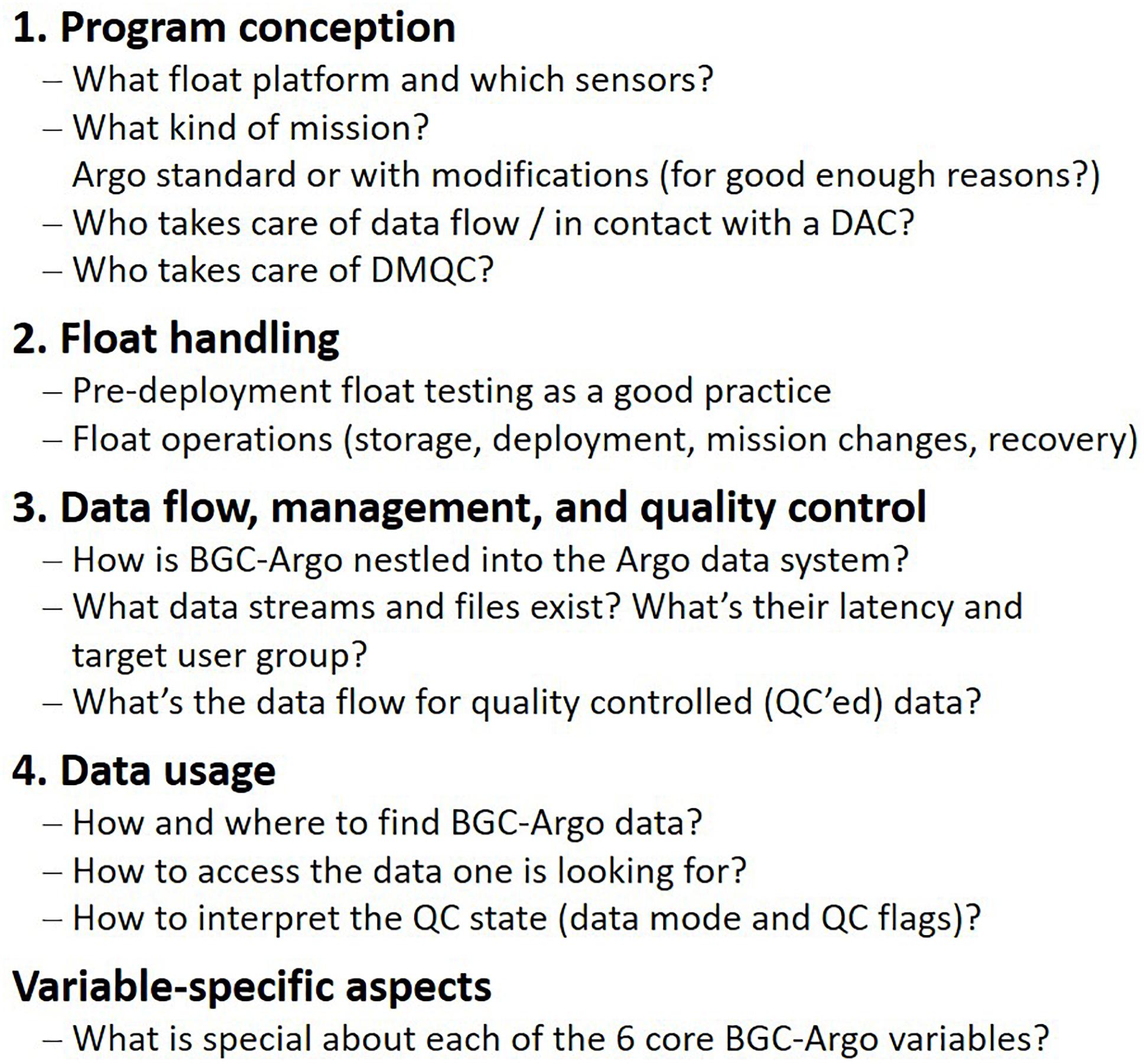
Figure 1. Key points and questions of a “BGC-Argo float life”, from conception, float operations, data management and quality control to data usage.

Up-to-date information on BGC-Argo such as participating countries and projects, BGC-Argo’s objectives, the network’s status, or links to the current data management documentation are available online at biogeochemical-argo.org.

1. Preparation and Deployment Conception

Mission Considerations or the Global Goal and the Compromises Required to Achieve It

To be a part of Argo, a BGC-Argo float mission must conform to the guidelines set out by the Argo Steering Team¹. A float included in Argo:

• must follow the Argo governance rules for pre-deployment notification and timely data delivery of both real-time and delayed-mode quality controlled data,

• must have a clear plan for long term data stewardship through a national Argo Data Assembly Centre, and

• should target the core Argo profiling depth and cycle time, 2000 m and 10 days, respectively. However, data that contributes to the estimation of the state of the ocean on the scales of the core Argo Program are also desirable.

These guidelines also define three stages in the expansion of Argo: Experimental Deployments, Global Argo Pilot, Global Implementation. BGC-Argo has achieved the second stage for its recommended core set of six variables (oxygen, nitrate, pH, chlorophyll fluorescence, optical backscatter, and solar irradiance). Those variables were chosen based on availability of operational sensors and desired research and management needs. To achieve the next stage, the BGC-Argo implementation plan targeted a fleet of 1000 floats profiling on average every 6 days, i.e., fewer than 1 float per 300 × 300 km area of ocean (Biogeochemical-Argo Planning Group, 2016). This was primarily based on an observation system simulation experiment (OSSE) designed to quantify the minimum number of observational platforms needed to constrain global air-sea CO₂ exchange (Biogeochemical-Argo Planning Group, 2016). Additional methods, such as satellite ocean chlorophyll data denial experiments, where an increasing part of the data are withheld and the difference between subsampled and full resolution field investigated, as well as a general evaluation of decorrelation length scales for various ocean variables, were assessed and resulted in a similar recommendation for array size. To support and sustain such an array size, float endurance and longevity are a crucial factor. If float lifetimes are shortened because of rapid repeated profiling, more BGC-Argo floats have to be deployed to maintain the array. The BGC-Argo implementation plan aims for a 250 cycle/4 year lifetime with an average 6-day cycle interval (Biogeochemical-Argo Planning Group, 2016). This more rapid repeat cycle than the 10-day core-Argo mission does come with costs that are challenging for maintaining a global array (Roemmich et al., 2019). In addition, specific scientific goals, regional issues, funding sources, and even sensor configurations may motivate different missions, and we illustrate these issues with two examples below. Addressing these issues is challenging, and achieving the greater goal of a sustained global array will require compromises. As a starting point, we suggest that participants in BGC-Argo should, at a minimum, commit to achieving the 10-day repeat cycle for a targeted lifetime of 4 years (i.e., 150 core BGC-Argo profiles over 4 years), profile down to 2000 m at least once a month, and target expending less than 20% of their float battery budgets addressing ancillary goals beyond the core BGC-Argo mission. Illustrative examples of the compromises required to meet specific science goals outlined in the BGC-Argo implementation plan include (i) the disparate optimal missions required for both the radiometer and chlorophyll sensors to contribute to the quantification of phytoplankton biomass and (ii) the measurement of net community production (NCP) using oxygen sensors.

Fluorescence observations as a measure of phytoplankton biomass are best done at night, because this signal is significantly compromised during the day by non-photochemical quenching (a response by phytoplankton to light that results in a reduction of fluorescence per unit chlorophyll, Kiefer, 1973). In contrast, assessment of biomass by the attenuation of the radiometer signal, and comparison of BGC-Argo sensor results to satellite remote sensing motivates measurements near noon. This combination merits obtaining both day and night profiles (IOCCG, 2011), and accordingly a mission with day-night pairs of rapid shallow profiles may be optimal. Interspersing these with deep profiles can meet core-Argo goals and also provide benefits for the bio-optical observations, because the increase in pressure significantly reduces the rate at which bio-fouling develops (Gould and Turton, 2006) and deep “spikes” in bio-optical signals are indicators of particle aggregates important to export processes (Briggs et al., 2011). Importantly, many BGC-Argo floats may not initially deploy both fluorometers and radiometers, and thus this type of compromise may not be required for all floats. Note, however, that performing measurements at a given time of day or night will bias our ability to study the relationships between diel mixed-layer processes and observed parameters.

The oxygen sensor is useful to assess both changes in global ocean oxygen inventories and local biological activity, e.g., NCP as the balance between photosynthesis and respiration (Biogeochemical-Argo Planning Group, 2016, and references therein). These different goals have different optimal missions. Changes in whole of oxygen inventories are expected on decadal timescales (Stramma et al., 2010; Helm et al., 2011) motivating sustained array observations and requiring significant commitment to sensor stability assessments (Körtzinger et al., 2005; Bittig and Körtzinger, 2015; Johnson et al., 2015; Bushinsky et al., 2016). Options for assessing stability include:

• Periodic deep profiling into waters where oxygen concentrations can be considered stable and known (i.e., correction to climatology) – data at 2000 m appears appropriate for this along with assumptions about how biases from deep values should be used to correct values over the whole profile (for example assuming a constant gain or constant offset or their optimized combination, Takeshita et al., 2013; Bittig et al., 2018a). Deep profiles are required often enough to repeatedly sample waters of relatively constant temperature (T), salinity (S), and O₂ properties relative to the shallower changes of interest, and thus the optimum frequency will depend on location.

• Use of a regional feature such as zero oxygen concentrations in oxygen minimum zones at mesopelagic depths as a special form of the climatological approach, without the requirement for as deep profiling (Wojtasiewicz et al., 2018b).

• Periodic measurement of atmospheric oxygen values using sensors that emerge from the sea, i.e., the optode on a stick approach (Bittig et al., 2015). In principle this is an improvement over deep climatological corrections, because the oxygen content of the atmosphere is spatially invariant relative to all ocean oxygen questions of interest and the sensor response is very sensitive at these levels, but is not achievable by all sensor types.

In contrast, NCP measurements, especially if they are to be scaled to satellite remote sensing of biomass to achieve global perspectives, require high temporal and spatial frequency observations, because NCP changes sign on diel cycles and control by zooplankton has shorter correlation length scales than the sub-mesoscale phytoplankton fields (e.g., Abraham, 1998).

In summary, float deployments often serve multiple purposes and careful compromises must be made. This includes the optimal choice of sensors and the optimal choice of missions. Interspersing mission types or changing missions over the lifetime of the float can be a useful strategy to address these compromises. This can include reacting to events over the lifetime of a float, such as drifting into shallow waters that preclude deep profiling or degrading responses from one or more sensors that motivate focusing on other goals than initially envisioned. All of these issues motivate committed ongoing involvement with float missions after deployment. Care must also be taken that these considerations do not become overly complicated but give full consideration to later data processing requirements, comparability to other floats and interpretability of data.

Data Management Considerations

Whether deploying a handful of floats or a larger array, giving adequate consideration to the structure of one’s data processing workflow in advance to float deployment is highly advised. Developing a working relationship with the local Argo Data Assembly Center (DAC) will serve to assist in this process, as each DAC acts as a gateway in the transfer of BGC data from float(s) to the Global Data Assembly Centers (GDACs). The float owner/principal investigator’s (PI’s) level of involvement/cooperation in float data processing and in the production of Argo-specific files can vary depending on availability of resources and personnel. However, certain issues, such as assigning a representative to manage delayed-mode quality control (DMQC) of core and BGC float data, will require some level of involvement on the float PI’s behalf. Additionally, it is worthwhile to anticipate the explicit needs of one’s user-base in the context of data management. For example, are there additional file formats or derived products (that fall outside of the Argo domain) that would be useful to one’s science team or external float-data users? If so, is there a potential avenue for production of such products within the operational data stream? Such questions are worthy of consideration as one plans a program and reaches out to one’s DAC representatives. Further details on such topics, including key recommendations with respect to data management and operations within the Argo system, are outlined in section “3. Data Management/Processing and QC.”

Platform Considerations

The specific float platform used is at the core of any BGC-Argo project. Different types of floats have different capabilities (e.g., number of sensors that can be accommodated, battery capacity, flexibility with respect to the frequency and vertical resolution of individual sensor measurements), which constrain how each sensor can be operated to achieve the required number of profiles.

At present, there are nine manufacturers whose floats have been equipped with at least one BGC sensor (Table 1). The three most common commercially available ones are the Apex, Provor, and Navis floats, for which Table 2 gives a more detailed overview with respect to various float capabilities. Among these, Navis floats are the most lightweight and easy to handle, and Provor floats are the most flexible and adaptable thanks to two controller boards, a board for float operations and a science board for the sensors. Float energy budgets and telemetry systems should also be thoroughly understood prior to float selection and mission planning. As an example, an estimation of power consumption per profile is given in Table 3 for an Apex-UW SOCCOM BGC-Argo float (after Riser et al., 2018) and an NKE PROVOR CTS4 remOcean BGC-Argo float. Additionally, Iridium rudics communication is typically more cost-efficient for BGC-Argo than Iridium SBD communication (Riser et al., 2018). The choice of float, however, depends on multiple criteria and should be made separately for each project.

TABLE 1

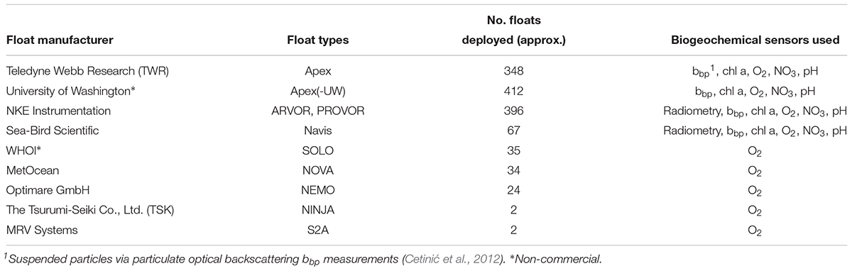
Table 1. Distribution of currently deployed BGC-Argo floats (as of January 2019) by float manufacturer/float type with list of biogeochemical sensors that have been used on these floats (not always concurrently). Information are compiled from AIC/JCOMMOPS and GDAC meta data.

TABLE 2

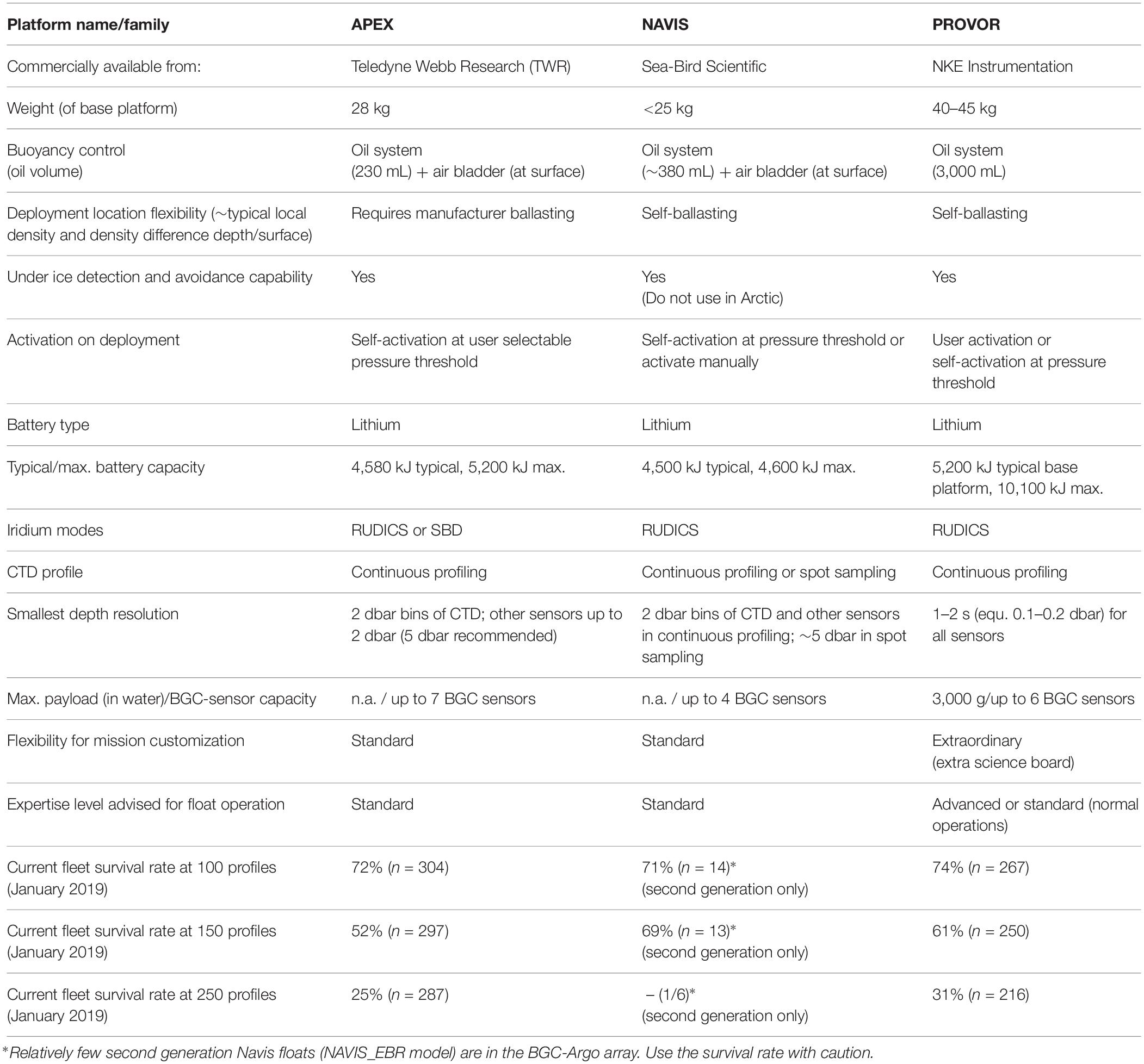
Table 2. Qualitative comparison of common, commercially available BGC-Argo float types.

TABLE 3

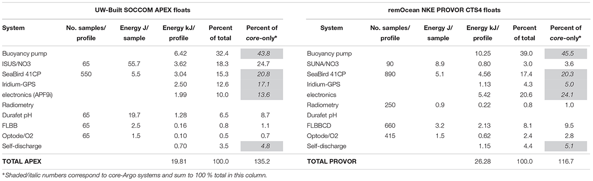
Table 3. Energy budget estimate on a per profile basis for UW-built SOCCOM APEX floats (left set; after Riser et al., 2018) and for remOcean NKE PROVOR CTS4 floats (right set; 2000 m profile). Total battery capacity for both floats is 5,200 and 8,600 kJ, respectively, which gives energy for nominally 262 profiles for SOCCOM APEX floats and for 327 profiles for remOcean PROVOR CTS4 floats.

2. Field Aspects

Pre-deployment Testing

BGC-Argo floats are complex instruments that merit pre-deployment qualification. In general, pre-deployment testing on the user side helps to increase confidence in float operation as well as to identify hardware and/or firmware flaws or glitches that may have catastrophic consequences if unnoticed. This may only affect a fraction of floats, but is important both on a fleet/network level and on an individual float level, given the investment of a BGC-Argo float.

Float manufacturers are expected to conduct similar tests prior to shipping floats to customers, to ensure proper functioning and best performance of their product. This is crucial to also enable contributions of small programs or individual researchers to the construction of the BGC-Argo network.

This section can only provide qualitative indications and few quantitative statements. The reason is that programs that deploy a certain kind of float in large numbers (i.e., with a sound statistical basis) tend to perform particular testing or adaptations to the floats since they have the necessary leverage, expertise and resources. For example, commercial TWR-built APEX floats and APEX floats built at the University of Washington (UW) have largely the same hardware. UW, however, intensively tests the hardware and float operations before deployment. In addition, UW also developed its own firmware that is different from TWR. Another example is the NKE Provor type of floats. The majority of floats (80% as of January 2019) pass through a pool test deployment (see below), allowing the identification and repair of malfunctions before deployment of both floats and sensors. The remaining ca. 20% of Provor floats pass through a test in an 8 m deep, water-filled basin at NKE, allowing verification of the float’s hydraulics. A comparison of float survival for these three sets of floats as well as Sea-Bird Navis floats is given in Figure 2. UW’s thorough testing and adapted firmware dramatically improves survivability when compared to other APEX floats. The survival rate of Provor floats is in between UW’s and other APEX float’s and shows a higher fraction of floats with many profiles. Statistics for Navis floats are less robust due to fewer deployed floats (Figure 2). Note that they include floats both from the first generation (“NAVIS_A” model) and current generation (“NAVIS_EBR” model), which received a major redesign of the air/oil bladder system, as well as floats that underwent additional checking at UW.

FIGURE 2

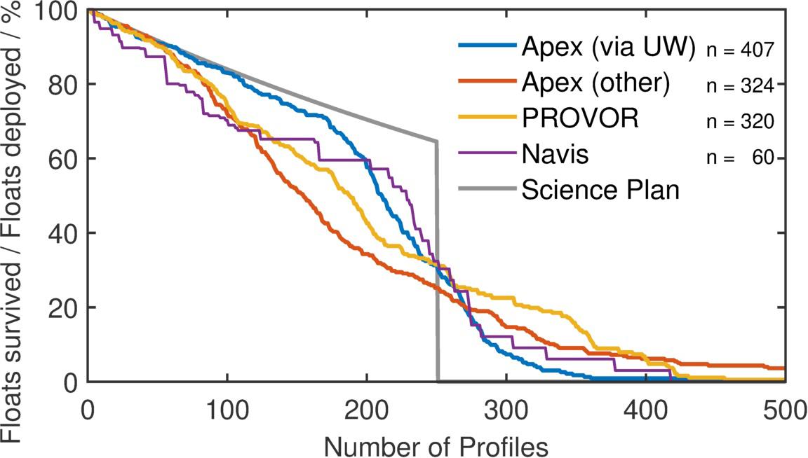
Figure 2. Float survival rate of Apex-UW (blue, n = 407) vs. other Apex floats (red, n = 324). Same for Provor floats (all types) (yellow, n = 320). Note that not all of the Provor profiles go down to 2000 dbar. Navis floats (both NAVIS_A and NAVIS_EBR models) are shown for completeness (purple, n = 60). About one third of the Navis floats underwent additional checking at UW. The gray line gives the float survival estimate from the BGC-Argo Science and Implementation Plan (250 cycle lifetime, average 6 days cycle interval, 90% survival rate per year; Biogeochemical-Argo Planning Group, 2016).

As a general rule, appropriate time and resources should be allocated for testing and qualification prior to deployment. Everything that is feasible to test should be tested, which may also depend on the particular float type. Guidance can be obtained from manufacturers as well as details on the tests performed prior to float delivery. The depth of tests ranges from those carried out in port and on the ship, where the least amount of time and facilities are available, to tests carried out at a home institution with engineering facilities, where one has the most time and tools to check out the float. For this purpose, engineering facilities include technical personnel, an electronics shop, saltwater pool and pressure test facilities. It is considered good practice to perform pre-deployment tests, including whole platform operation “dock tests”/pool or at sea tests whenever firmware is changed significantly.

Part of (in lab) pre-deployment operations should include the completion and archival of all float-related metadata, including battery type and capacity, float and sensor types as well as serial numbers, and vertical offsets of BGC sensor positions relative to the pressure sensor, due to their attachment location (see Supplementary Material for an example). Ideally, these metadata are supplied by the float manufacturer.

Example: University of Washington Float Qualification

In principle, there are three levels of float testing: (A) In lab (with engineering facilities and time prior to shipping), which include all tests of (B) and (C) (see Figure 3). (B) In lab (no engineering facilities, with time prior to shipping), which include all test of (C). (C) In port or on research vessel (no engineering facilities, limited time before deployment).

FIGURE 3

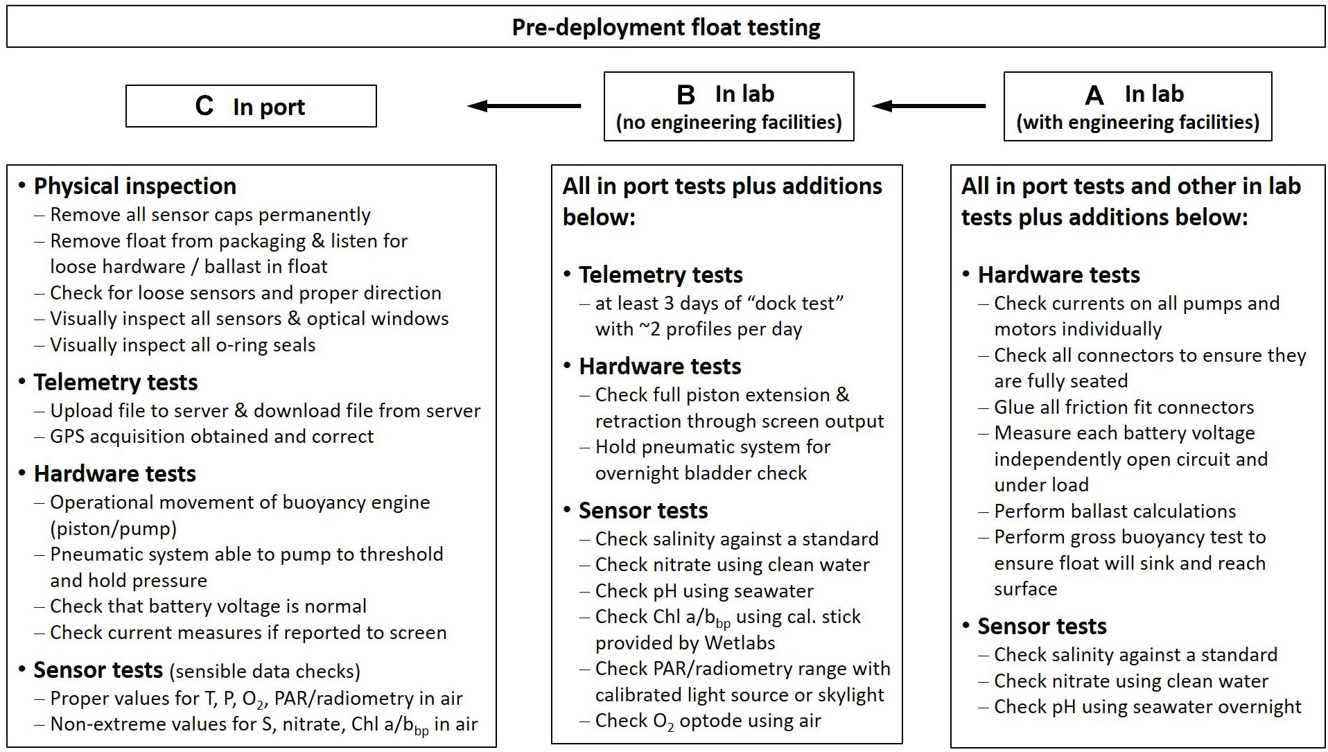
Figure 3. Pre-deployment float testing levels with steps undertaken based on University of Washington experience. Whether all three levels of float testing (A–C) can be performed depends on facilities and time available prior to deployment.

The tests of level A, in essence, control all movable parts of a float. For “dock testing” (level B), the float is put outside where satellite communication and GPS acquisition is possible. It then starts a “normal” mission, including buoyancy engine actions, satellite communications, and the sensors are sampled at least once as the float crosses one pressure table sample over multiple days of testing. It is set to cycle rapidly (e.g., 2 profiles per day) to verify normal float functioning. The in-port tests of level C are simple but nonetheless crucial to catch any issues which occur during shipping and should be standard practice for all deployments. Due to the large number of sensors on these floats, they are very susceptible to damage in transit.

Example: Ifremer Pool Float Tests

Once sensors are individually tested and then mounted on the float, PROVOR BGC Argo floats undergo a pool test in the Ifremer pool (20 m depth, 50 m length). Each float slides along a line which is stretched between the bottom and the surface. The distance between the vertical lines is less than 1 m (Supplementary Figure S1). The pool is supplied by sea water, which is filtered and treated by additional bleach injection. The floats are launched like they are in an at-sea mission. They perform several cycles (typically 3). Parameters are measured at first descent, at the park depth (20 m), and during the ascent. These tests are a crucial way to identify and avoid bugs in new firmware pre-deployment.

Additionally, tests at sea can be made, e.g., off the bay of Villefranche-sur-Mer given easy access to deep water. The float is attached to a line with a buoy at the surface, and can profile from 0 to 200 m (see Table 4 for a pros and cons of such tests).

TABLE 4

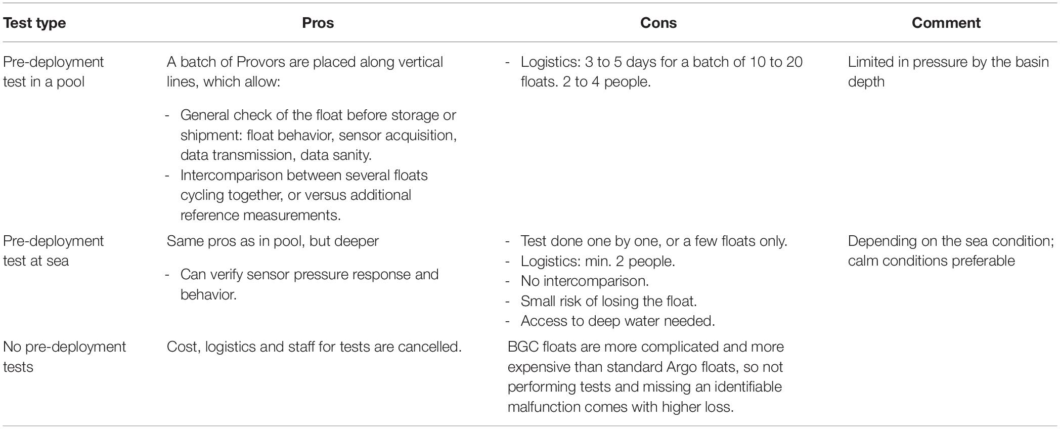
Table 4. Comparison of float test deployment options with pros and cons based on Ifremer experience.

Float Storage

During storage or transport, freezing temperatures should be avoided. If the float is expected to encounter freezing temperatures, the conductivity-temperature-depth sensor (CTD) and pumped flow paths must be dried before shipment to avoid cracking of the conductivity cell. This holds true during shipping, home institution storage, or storage while on the deck of the ship before deployment. When preparing the float for deployment in such conditions, the float must be inside the ship and the deployment phase should be as short as possible (e.g., less than half an hour). Using insulated protection around the float and the sensors can be a way to limit thermal effects. Extreme temperatures (both high and low) can have an impact on the float calibration due to the acceleration of the deterioration of the filter of the radiometer, for example. The loss of energy from the main battery during storage is temperature dependent, with a typical self-discharge rate of 3% per year (Riser et al., 2018). Higher temperatures lead to an increase in self-discharge. This behavior is not specific to BGC floats.

Float Notification and Argo Governance

Since 2000, the implementation of the Argo program has been guided by IOC/UNESCO Member States and a set of resolutions (XX-6 and EC-XLI.4) and guidelines to meet coastal states legitimate transparency demand in the United Nations Convention on the Law of the Sea (UNCLOS) context. Resolution XX-6 (IOC, 1999) requested Argo implementers to notify, reasonably in advance and through appropriate channels, any Argo float deployment in the high seas that might drift into Member States exclusive economic zones (EEZ). Resolution EC-XLI.4 (IOC, 2008) offered then the possibility to coastal states, through official request to IOC/UNESCO, to be formally and bilaterally notified of float drift into EEZ by implementers. This resolution and resulting guidelines clarified as well the right for the coastal state to request to stop data transmission in its EEZ. These rules apply to official Argo floats, endorsed by the Argo Steering Team, and not to any profiling float.

The Member States of the Intergovernmental Oceanographic Commission of UNESCO have agreed with Decision EC-LI/4.8 (IOC, 2018) to have BGC-Argo floats and their 6 core variables covered by the same notification regime as core Argo floats. This requires as well free and unrestricted data sharing in real-time; a mandatory rule for all Argo floats.

Practically, all BGC floats deployed in high seas, which might drift into Member States EEZs, will not require a clearance according to UNCLOS, but rather a bilateral notification from the implementer to the coastal state. Such notification is triggered by a real-time warning system set up at JCOMMOPS and its Argo Information Centre (AIC)², which assist implementers to do so and concerns for now a dozen of coastal states. However, all Argo implementers have to seek a Marine Scientific Research (MSR) clearance (according to UNCLOS) for deployment of floats directly into EEZs for most of the Coastal States.

Any BGC-Argo float deployment needs thus to be notified with the AIC in advance of deployment. The AIC developed a centralized electronic notification system, which informs Member States of the float deployments. Float operators register their deployment (including early plans) in the AIC system, which will trigger a notification email including float deployment details, sensors equipped, configuration, contact points, etc. The availability of data is also checked by the AIC. In this process, each Argo float deployment will be assigned a unique identifier, its WMO number, which is also used in the data system.

Biogeochemical float deployments outside of Argo (and outside the Argo data system) are possible and fall under the rules of UNCLOS. This means that MSR clearances will have to be requested to coastal states in advance (i) for deployments into any EEZ and (ii) for drift into any EEZ.

Float Deployment

Float manufacturers follow different deployment philosophies.

• Provor: Provor floats need to be shipped with their batteries in switch-off state because of transport regulations, which requires an operator to switch them on prior to deployment. NKE floats are adjusted to maximum buoyancy before deployment (i.e., the float is shipped with its external oil ballast full) to prevent the accidental sinking and loss of an inactivated float. To be able to sink, these floats must reduce their volume (buoyancy) by opening a solenoid valve to bring the oil back into the hull. Activation is typically done just before deployment. The float then starts a sequence of self-tests which last a few minutes with success indicated by an audible signal, signaling that the float starts its volume reduction. This volume reduction and signal lasts 30 min and the user should not deploy the float after the signal has stopped to avoid too rapid sinking of the float. After deployment, it can take 30–40 min before the float leaves the surface, possibly longer in cold waters due to increased oil viscosity.

Alternatively, recent Provor floats can be activated in advance with a pressure threshold triggering the start of the mission (compare Apex/Navis behavior below), though this procedure is not recommended by NKE.

• Apex/Navis: Navis floats are shipped in a “frozen” mode and need to be connected to a computer using the serial (20 mA) connector to wake up (the magnetic interrupt switch cannot be used to wake up Navis floats). For APEX and Navis floats, startup can be done well in advance of actual deployment (e.g., in port). The float then reads its pressure sensor every 2 h. As the float is ballasted low, it sinks (passively) on its own, and typically leaves the surface after the cowling fills with water (2–20 min). When the float’s pressure reading exceeds a 20 dbar threshold, the float starts its mission (“pressure activation”).

Pre-deployment sensor-specific procedures should include the cleaning of optical windows (e.g., Talley et al., 2017). Upon deployment, metadata should be completed with location, time, concurrent observations, etc. (see Supplementary Material for an example).

Concurrent reference samples (e.g., calibrated CTD-O₂ cast; bottle NO₃, pH, chl a, HPLC pigments, POC samples; sensor chlorophyll a fluorescence, b_bp, radiometry profile) are taken by many groups. This is good practice and recommended for validation, but not essential for calibration in most cases, see section “Variable-specific Aspects”.

Mission Modifications

Experience from some float groups suggests that daily profiles for the first 5 days after deployment as well as enabling descending and ascending profile acquisition (only possible on NKE floats) allow certain sensors (e.g., pH, O₂) to stabilize faster for better calibration against ship data. After these 5 days, the float can be configured to a standard Argo mode. This includes profiling to 2000 m depth at least once per month to allow appropriate salinity data qualification for the core Argo mission³.

Thanks to two-way communication, mission changes like those above are possible during deployment. This is a very useful capability, but should be used cautiously, depending on the detail of modification. If the level of the modifications is low and affects only standard parameters (e.g., float profiling or parking depth, cycle period), they can be easily changed. For example, the remOcean project floats in subpolar/austral areas follow a spring/summer bloom period-intensified schedule (i.e., cycle interval of 2 days in December–February, 5 days in March/April, 10 days in May–August, 5 days in September, and 3 days in November, respectively). More advanced modifications, that may not be available on all float types, include individual sensor on/off depths or sampling frequencies (e.g., possible on NKE, Apf11 floats). Other parameters can be very advanced and should be left to expert users.

In any case, any modification of parameters must be carefully checked in order to detect any conflict between them. Pre-validated missions should be used or, if available, a simulation software that assists the float operator in this task. The new mission parameters are directly connected with the firmware version of the float, i.e., the float version must be kept in the meta data. This information is crucial. The capability to change the float mission can become quite time consuming because the data subsequently transmitted by the float needs to be monitored frequently.

Float Recovery

This is only possible with two-way communication which permits a change in mission parameters to set a float into recovery mode. This mode keeps the float at the surface sending regular position updates at a higher frequency. BGC-Argo float recovery is becoming a common practice when logistics permit, e.g., in the Mediterranean or Baltic Sea, and allow post-deployment verification and recalibrations of sensors.

In the Baltic Sea, a permanent presence in the Gotland basin has been maintained by Argo Finland since 2013 using 2 floats interchangeably (Siiriä et al., 2018). The NAOS Mediterranean array has been maintained since 2012 with about a dozen active BGC-Argo floats and a total fleet of 30 BGC-Argo floats. Every 2–3 years, a ship cruise is dedicated to the recovery of old floats and the deployment of refurbished platforms (Taillandier et al., 2018; D’Ortenzio et al., in preparation). Recovered floats have been refurbished in the following way, serving as a template for others: Visual check of the sensors before cleaning, systematic replacement of batteries and o-rings in the lab, pre-deployment tests for ballasting, communication, mission configuration and software performance. In addition, sensors should be recalibrated as a best practice recommendation. Calibration/validation was performed during (re-)deployment using water samples of a concomitant CTD and bottle sample cast.

Recovering and redeploying floats is cost effective, eco-friendly, allows for sensor recalibration, and helps to maintain the BGC-Argo array and attain the BGC-Argo science goals (Biogeochemical-Argo Planning Group, 2016). It is thus recommended to check for recovery opportunities wherever possible. Note, however, that while float recovery and redeployment has many benefits, its feasibility is highly dependent on float location and related field logistics and is not mandatory within the Argo system. Only 4% of the current BGC-Argo array has been successfully recovered (as of January 2019), the majority of which were deployed in semi-enclosed seas.

The NAOS redeployment experience suggests that though the recovered battery voltages would allow a prolonged deployment, the bio-optical sensors were covered by a biofilm in most cases (depending on in situ conditions encountered), which decreased the data quality and became the factor limiting the mission. In contrast, optics and electronics of the bio-optical sensors were not critically affected even with high sampling rates. Overall, the choice to limit the deployment of the platform to 2–3 years (about 200 cycles) provided a better data quality and reduced calibration drifts. On the other hand, the floats’ technical functioning or battery lifetime was not limiting the missions. When seen in the perspective of maintaining the array, the recovery cruise allowed for a higher level of data quality and maintained the initial seeding plan for the Mediterranean.

3. Data Management/Processing and QC

Placement Within the Argo Data System

The primary objective of BGC-Argo data management is to provide calibrated, science-quality biogeochemical data to the global user community, while at the same time preserving raw BGC float data in its original form such that applied adjustments can be reprocessed as-needed. The pre-existing framework of the core Argo data system supports these aims through the management of specific real-time and delayed-mode file structures. Additionally, associated meta-data, trajectory, and technical files provide the supporting framework for storing all pertinent calibration and location information.

BGC-Argo data are nested within the core Argo data system, and preserve all float data needed for “from-scratch” reprocessing. To increase biogeochemical data visibility and availability, it is therefore “best practice” to serve these data within the pre-established Argo data system. The Argo data system has been serving core Argo data successfully since 2001 and is considered a reputable repository for data from autonomous profiling floats. Since biogeochemical data are obtained by sensors that are housed within Argo floats and need to be used in conjunction with their temperature (T) and salinity (S) profiles, it is natural to serve the BGC data as an extension in the core Argo data system.

An “extension” format has been designed that allows biogeochemical data to be served within the Argo data system, and yet leaves the core Argo component undisturbed. This is achieved by storing T/S data and BGC data in two separate files, a core- and a b-file. BGC data generally require more frequent delayed mode assessment and reprocessing than their T/S counterparts simply due to the relative immaturity of the sensors. The 2-file structure means that the relative instability of the BGC data will not disturb the stability of the T/S data. Hence on occasions when the BGC data undergo significant changes, the T/S component can continue to function independently in order to serve its core users.

The core-file stores the pressure, temperature and salinity data. The b-file stores the pressure and all corresponding BGC data. The pressure axes in both files are identical and are used to merge core and BGC data from a single cycle into various higher-level files served at the GDAC. All the profile data are stored as they are telemetered and decoded, thus preserving the data in their rawest form. In the b-files, both the intermediate BGC parameters and the computed ocean-state BGC parameters are recorded. In this manner, re-processing of BGC data can be carried out with relative ease and integrity.

In addition to the single-cycle vertical profile files (core- and b-), other float data are stored in composite multi-cycle files: _traj, _meta, _tech. Together these files serve to preserve the complete float record.

Data Processing and Quality Control

Being part of Argo, BGC-Argo has two data streams: “real-time” and “delayed-mode.” The real-time stream has a latency requirement of 24 h between profile termination and data availability at both GDACs. Real-time data are aimed to serve operational users such as those assimilating Argo float data within numerical weather prediction and other operational models. Data in this stream is subject to real-time quality control checks and is expected to be free of gross outliers. Only automated quality control and data checks can be applied. The second data stream, delayed-mode data, is meant to provide the best quality data for science at the present date, including realistic error estimates. It includes more sophisticated data adjustment and quality control procedures than the real-time data stream, including manual inspection by either the float’s PI or pre-identified DMQC expert. For core data, the DMQC process is typically expected to occur on an annual basis. The same frequency is recommended for BGC parameters, although initial DMQC, which improves initial accuracy considerably, should be performed as soon as a sufficient number profiles have been returned (typically after 5–10 cycles). The sequence of DMQC actions and its impact during float’s life time is illustrated in Figure 4. During a delayed mode assessment, for either core or BGC data, data from a float are rigorously examined in a multi-parameter context, which typically includes some level of comparative analysis to regional reference data and climatology (e.g., Wong et al., 2003; Owens and Wong, 2009; Johnson et al., 2017). In many cases, any necessary data adjustments (gain, drift, offset) derived by the delayed-mode operator during such an assessment can be fed back into the incoming data stream in real-time, producing real-time adjusted data. The data stream associated with each float parameter, whether real-time (R), real-time-adjusted (A), or delayed-mode (D), is recorded within the PARAMETER_DATA_MODE variable in the files. The file name prefix contains a “D” if any of the float’s parameters are in delayed-mode. If no parameters exist in delayed-mode (i.e., all parameters are either real time, “R,” or real time adjusted, “A”), then the file name prefix remains “R” (Table 5).

FIGURE 4

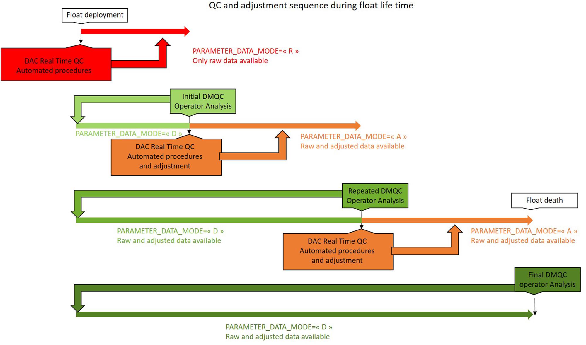
Figure 4. Sequence of quality control and adjustment steps during the life time of a float from float deployment to death. The color shading indicates the data mode: “R” real-time data in red, “A” real-time adjusted data in yellow, and “D” delayed-mode data in green. Initial DMQC should be performed soon after deployment (typically after 5–10 cycles). With subsequent DMQC revisits (on an annual basis), adjustments become more reliable (indicated by the green shading).

TABLE 5

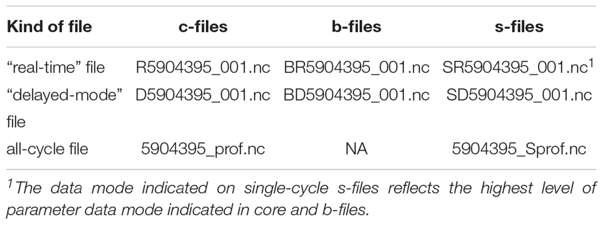
Table 5. Example of the file naming scheme for a float with WMO number 5904395. Note that either a “real-time” c-/b-/s-file or a “delayed-mode” c-/b-/s-file exists, not both. The all-cycle file contains all available cycles for the float.

These two data streams are reflected in the BGC-Argo data processing organization and documentation. A total of 9 out of the 11 Argo DACs process BGC-Argo parameters, <PARAMs>. The DACs receive float-transmitted raw or preprocessed sensor data, such as sensor counts or voltages (termed intermediate or “i”-parameters), and translate them to ocean-state biogeochemical quantities held in Argo “b”-parameter variables (i.e., DOXY, NITRATE or CHLA). This step is the “bread and butter” of a DAC, and all processing formulas are detailed in a “Processing BGC-Argo <PARAM> data at the DAC level” cookbook for each parameter (e.g., Table 6, column 2 for an overview) with an update frequency that follows approximately the inclusion of a new sensor into BGC-Argo. Each cookbook document is highly comprehensive, often including sample parameter data processing code and meta-data population examples for a wide range of BGC sensor types and model configurations. It is highly recommended that particular care is taken in following the procedures outlined within the Argo data processing documentation in order to ensure consistency between DACs. Specific questions related to a specific float configuration, should they arise, are typically directed toward the Argo community via the Argo data management list-serve.

TABLE 6

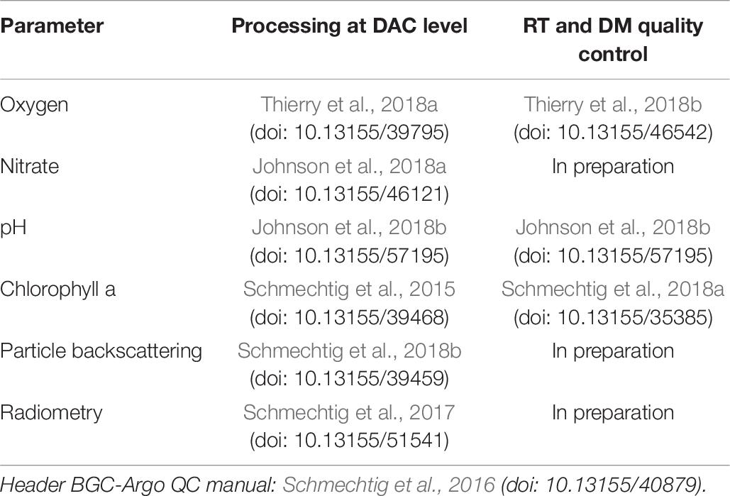
Table 6. Overview about BGC-Argo documentation for the 6 core BGC variables.

It is important to note that the accuracy of “R”-mode BGC data resulting from the cookbook processing is often not suitable for direct usage in scientific applications due to the presence of potentially large initial offsets, the magnitude of which cannot be fully characterized prior to deployment. Therefore, users are warned that raw biogeochemical data should be treated with care, and that often, adjustments are needed before these data can be used for meaningful scientific applications.

This is why there is a second BGC-Argo document for each parameter, an “Argo quality control manual for <PARAM> data” (e.g., Table 6, column 3 for an overview). The QC manuals go hand in hand with the processing cookbooks. However, their update frequency is driven by scientific evolution. Each QC manual details parameter-specific QC tests applicable to “R”-, “A”-, and “D”-mode data. Moreover, they describe the adjustment procedures required to make the biogeochemical quantities scientifically usable, both in delayed-mode “D” (using potentially complex methods) and in real-time adjusted mode “A” (using robust and operationally feasible methods that do not require human intervention and are implementable at the DAC level). A real-time “A”-mode adjustment for incoming data can be based on a delayed-mode “D” adjustment of existing data. Both “D”- and “A”- mode data fill the <PARAM>_ADJUSTED data fields as well as the corresponding SCIENTIFIC_CALIB data fields. <PARAM>_ADJUSTED_ERROR estimates are mandatory for “D”-mode data and highly recommended for “A”-mode. If not stated otherwise, they represent a 1 sigma uncertainty. Note that raw intermediate parameters are not quality controlled and that only the derived BGC parameters receive QC.

Data Flow Guidance

Real-time operations, including the reception of float-transmitted files, decoding and conversion to biogeochemical parameters, application of real-time adjustments, as well as the creation of Argo netcdf files and transfer to the GDACs, are performed at each DAC.

Delayed-mode operations (data adjustment to science quality by an expert of the parameter, control and/or correction of QC flags, visual QC, incorporation of the results into the Argo files, and feedback of “D”-mode data files to the responsible DAC) fall exclusively into the responsibility of the float PI, and it is the float PI’s task to allocate appropriate capacity and funds to perform these tasks for the lifetime of the float.

Note that both the sharing of data and providing delayed-mode quality controlled data is mandatory for a float running under the Argo label and its associated IOC regulations (Argo Steering Team, 2018^{4, 5}).

Defining the proper pathway for processing of a BGC float (Figure 5) could take different forms, but having a system identified prior to deployment is advised. Suggested steps would include:

FIGURE 5

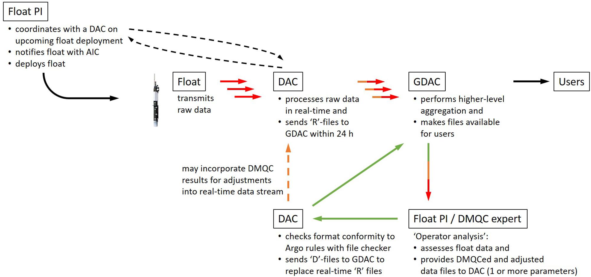
Figure 5. Pathway for processing of BGC-Argo float data with interactions and data flow between different players: float principal investigator (PI), data acquisition center (DAC), global DAC (GDAC), delayed-mode quality control operator, and users. The upper row indicates the real-time data stream, while the lower loop shows the delayed-mode data stream. All data are made available to the users via the two GDACs, ftp://ftp.ifremer.fr/ifremer/argo/ or ftp://usgodae.org/pub/outgoing/argo/.

(1) Identification of a pre-existing DAC to perform the real-time processing and submission of incoming float data in the proper Argo data-file formats.

(2) Identification of personnel to perform DMQC for core, and BGC data (This could include the float PI, or external experts. Given the richness of parameters, this does not need to be localized at a single laboratory).

An operational workflow must be established such that any data adjustments resulting from DMQC efforts (2) are effectively fed back into the processing and submission scheme (1). Key resources for aiding in the operational implementation of both real-time and delayed-mode processing, including specifics related to conversion of raw sensor output into scientific quantities as well as quality control and adjustment procedures, can be found at http://www.argodatamgt.org/Documentation, and are summarized in Table 6. Code/software that can aid in the QC process are, for example, the SOCCOM Assessment and Graphical Evaluation tools⁶ or Scoop-Argo (Detoc et al., 2017).

The Argo Data Management Team coordinates and approves the BGC-Argo processing and QC/adjustment approaches on the network level through the two key documents, the BGC-Argo cookbooks and the QC manuals, in order to ensure consistency between DACs/float operators and to incorporate and approve new scientific approaches.

Finally, as highlighted in the previous parts, the BGC-Argo data flow implies a lot of transformation of the data files from the real time to the delayed mode status. A file checker is developed and made available to the Argo community⁷ so that before submitting modified files to the GDAC, anyone can check that their files are compliant with the Argo rules and documentations.

4. Data Usage

File Types: Core-, b- and s-Files

There are three types of Argo files on the GDACs: (1) the core- or c-files; (2) the biogeochemical- or b-files; and (3) the simplified- or s-files (Table 5).

The c-files contain the float pressure, temperature and salinity data. The b-files contain the pressure and all BGC data, including the raw intermediate sensor data and the computed ocean-state variables. The c- and b-files record the raw float-transmitted data. However, there are subtle differences between how various float types/manufacturers/firmware transmit their data. For example, NKE PROVOR floats transmit the exact pressure reading at the moment a BGC parameter is sampled, while APEX floats transmit only the pressure at which a sequence of sensors samplings are initiated, i.e., all samples around a pressure level are reported with the same pressure despite being sampled at slightly different moments.

To (a) give a homogeneous structure to all BGC-Argo floats, independent of the level of detail of their transmitted data, (b) account for vertical displacement between T/S and BGC sensors due to different vertical position on the float, (c) co-align quasi-concurrent BGC observations for easy multi-parameter analysis, the c- and b- profile data are synthesized to produce the so-called simplified- or s-profiles at the GDACs (Bittig et al., 2019). The s-files contain both the T/S profile data and the ocean-state BGC parameter data interpolated onto one pressure axis. These are relatively new files in the Argo data system and will eventually replace the previous GDAC merge- or m-files, which were a simple concatenation of the T/S and BGC data without vertical interpolation.

Data Modes and Quality Flags

Biogeochemical-Argo data come in one of three data modes (Figure 6). These are given within the PARAMETER_DATA_ MODE variable and provide an indication on the data quality to expect:

FIGURE 6

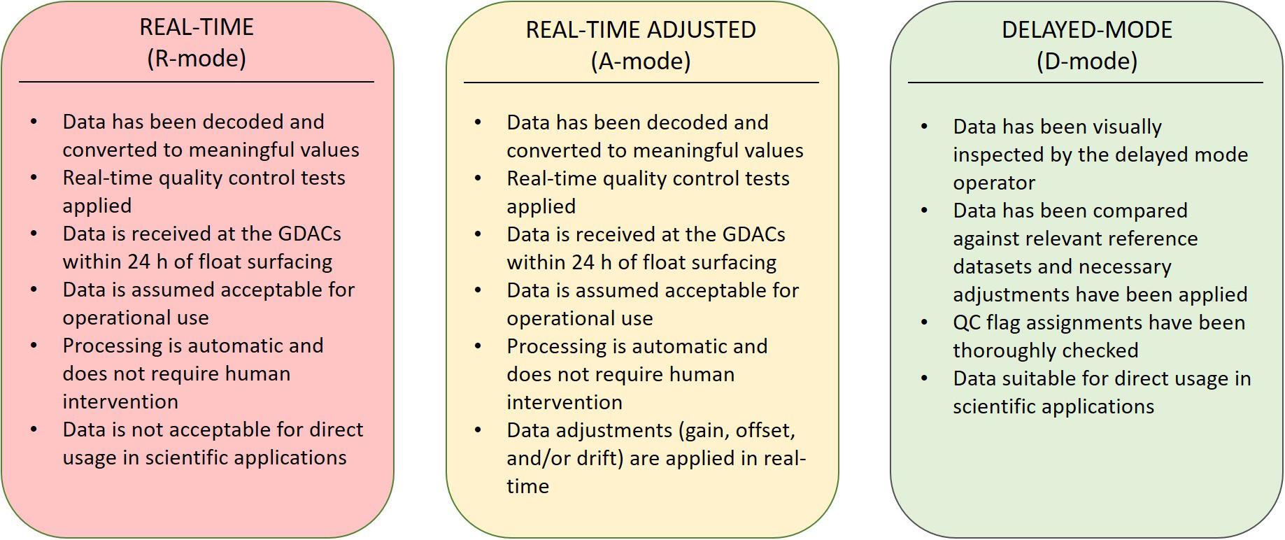
Figure 6. Summary of data mode characteristics.

“R” or “Real-Time”: Designates data of the real-time data stream that is unadjusted. These data were converted by the DAC from raw transmitted sensor data to an ocean state BGC parameter without any further adjustments. While real-time QC was applied to remove gross outliers, these data should be treated with care, as adjustments are often needed before these data can be used for meaningful scientific applications.

“A” or “Real-Time Adjusted”: Designates data of the real-time data stream that is adjusted in real-time. These data were converted by the DAC from raw transmitted sensor data to an ocean state BGC parameter and subsequently received an adjustment in an automated manner. While accuracy of such data is a priori much better than for “R”-mode data and should allow scientific use, no guarantee is given that they are free of sensor malfunction or other flaws (e.g., unidentified biofouling causing drifts/offsets). They can be provided with an uncertainty estimate (typically 1 σ).

“D” or “Delayed-Mode (Adjusted)”: Designates data of the delayed-mode data stream that have been adjusted (Note: Could be x + 0 if the raw data are fine) and quality controlled (e.g., flagging of data biased by biofouling; see details in QC manuals, Table 6) by a scientific expert. “D”-mode data are validated for scientific exploitation and represent the highest quality of data at the given point in time. They are provided with an uncertainty estimate (typically 1 σ).

Note that BGC-Argo is an evolving network, which is also true for its data. This means that “D”-mode data do not always stay the same. They may well change when better methods, climatologies, or longer float time-series become available.

In addition, each sample has a corresponding quality flag. The QC flags and their meaning are defined in Argo reference table 2 (Wong et al., 2019), reproduced in Table 7. The QC flags are an essential part of the data.

TABLE 7

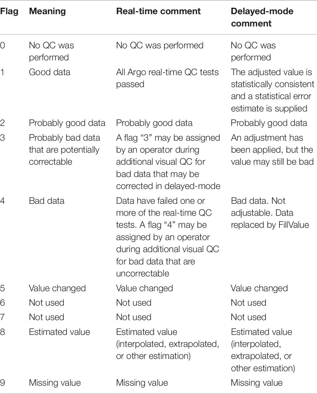
Table 7. “Argo reference table 2” with meanings of quality control flags from the Argo QC manual (Wong et al., 2019).

Data Access Guide

Data access begins with the search for appropriate floats and profiles. A good starting point is the exploration of various Argo index files at the GDACs, e.g., argo_bio-profile_index.txt lists profile location, time, parameters, and parameter data modes for floats at the GDACs.

Once identified, data access for individual files should follow:

(1) What parameters are in the file? (→ PARAMETER variable),

(2) What’s the processing state (“R,” “A,” or “D”) of the respective parameter? (→ PARAMETER_DATA_MODE variable), and

(3) Depending on (2), the actual access to both the parameter values and their quality flags (<PARAM> and <PARAM>_QC variables for “R,” <PARAM>_ ADJUSTED, <PARAM>_ADJUSTED_QC, and <PARAM>_ADJUSTED_ERROR for “A” and “D”) (Figure 7).

FIGURE 7

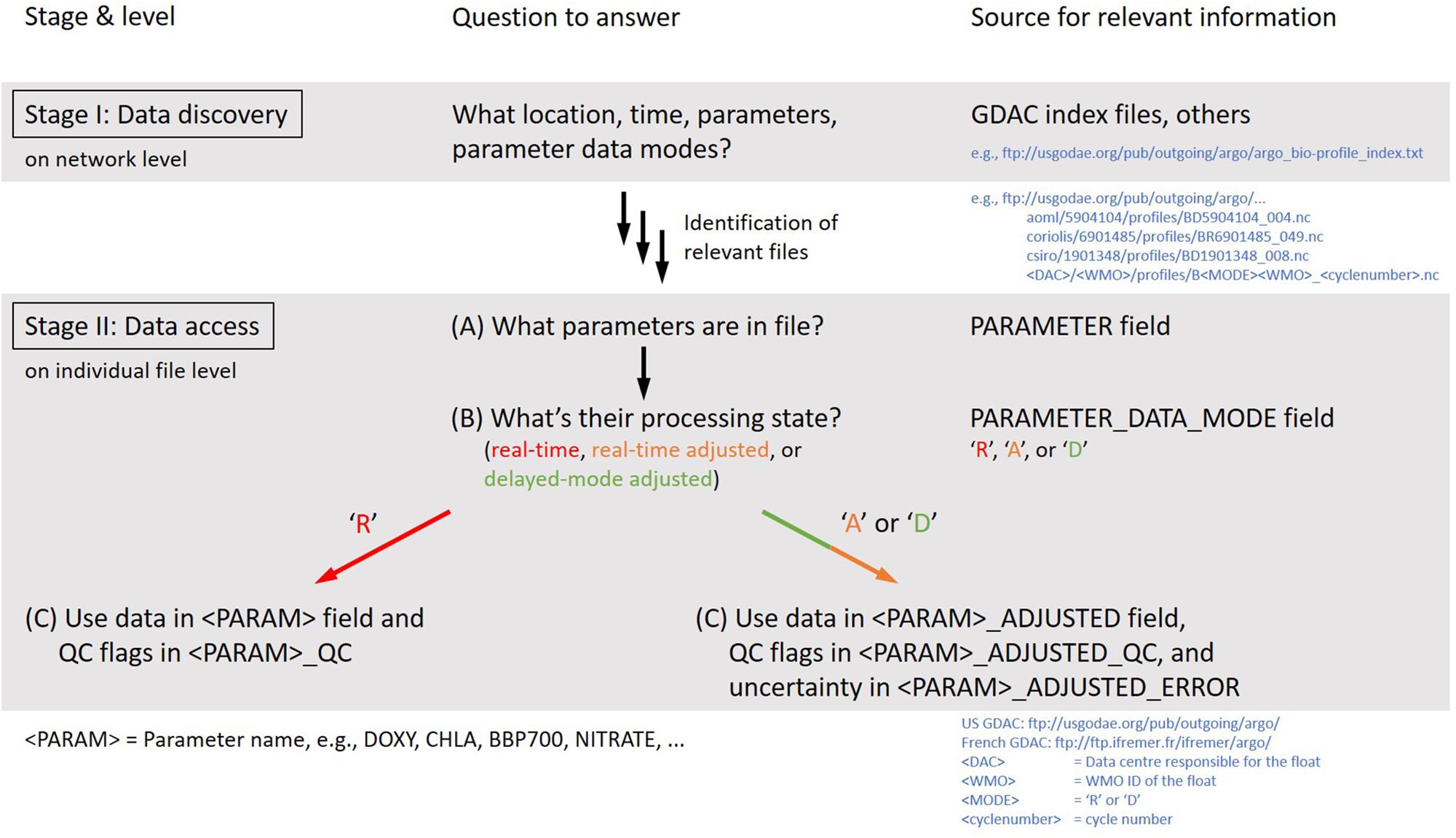
Figure 7. Workflow how to discover (stage I) and access BGC-Argo data (stage II).

Data Sources

Argo data can be accessed by either one of the two GDACs (ftp://ftp.ifremer.fr/ifremer/argo or ftp://usgodae.org/pub/outgoing/argo) or through the Argo GDAC doi (Argo, 2000). To allow traceability of research, the Argo doi may be sub-referenced to one of the monthly snapshots with its own doi key⁸.

Other sources may aggregate Argo data for specific purposes (e.g., regional). However, only those sources should be used where the data origin is traceable and transparent, i.e., a given profile can be unambiguously traced back to the Argo data system’s profile (i.e., has float WMO, cycle number, and file update date or Argo snapshot doi).

Data Acknowledgment

Being part of Argo, BGC-Argo data are freely available without restrictions. Still, Argo (and thus BGC-Argo) asks users to acknowledge their usage by stating “These data were collected and made freely available by the International Argo Program and the national programs that contribute to it (http://www.argo.ucsd.edu, http://argo.jcommops.org). The Argo Program is part of the Global Ocean Observing System.” and by citation of the appropriate Argo doi.

In many cases, however, the float PI or operator may have more detailed knowledge about a BGC-Argo float or the area of operation. For regional studies or studies involving just a limited number of float programs, it is recommended to contact the respective float PI or programs.

Variable-Specific Aspects

Descriptions of biogeochemical sensors available on BGC-Argo floats are provided below. Note that accompanying temperature, salinity and pressure data are required to support the transformation of raw data returned from a respective BGC sensor into a meaningful BGC quantity. The CTD instrumentation used on typical Argo floats is described in Roemmich et al. (2004). An outline of the associated core-Argo variable quality control procedures can be found in Wong et al. (2019). Such details will not be summarized here, as they are beyond the scope of this paper.

For all sensors it is good practice to always transmit the raw data, following the sensors’ sensing principle (e.g., temperature, phase shift, spectral absorption, currents, counts). The processing capabilities of the data management system will always be superior to on-board capabilities and raw data can be reprocessed at any time as improved algorithms become available as long as the calibration information is available. Figure 8 gives some examples of BGC sensor attachments on different float platforms.

FIGURE 8

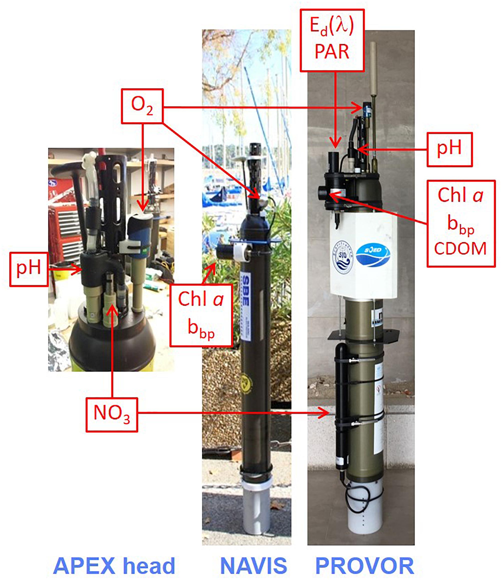
Figure 8. Examples for biogeochemical sensor attachments and implementations on different float platforms. Note that BGC sensors can be vertically displaced relative to the CTD pressure sensor. This displacement should be recorded in the float’s meta data.

Oxygen

Dissolved oxygen (O₂) is a key variable of ocean biogeochemistry (e.g., biological production, respiration) and a valuable tracer for ocean physics (e.g., ventilation, deoxygenation). It was the first biogeochemical variable to be measured by Argo (Körtzinger et al., 2004; Gruber et al., 2007).

The preferred type of sensor to measure O₂ from floats are oxygen optodes as they are robust and have low power consumption (order 1.5 J per sample). They are based on luminescence quenching of a chemical immobilized in a gas-permeable sensing membrane, which is in contact with seawater. This has two consequences: (1) Oxygen optodes sense the seawater oxygen partial pressure, pO₂, and (2) they show an oxygen time response due to re-equilibration between sensing membrane and seawater (Bittig et al., 2018a). Typical response times are between 5 and 100 s, depending on sensor and setting, and can be reduced if the optode is in a pumped flow (Bittig et al., 2014; Bittig and Körtzinger, 2017). Response time correction algorithms require the measurement times of optode samples to be stored and transmitted by the float’s firmware. The Argo data system is able to store this information alongside the sensor data (Bittig et al., 2017).

Only oxygen optodes with individual multi-point calibration should be used, as “foil-batch” calibrations perform worse in characterizing the O₂-temperature-response (Bittig et al., 2018a) and miss the accuracy target of 0.5% O₂ saturation (Bittig et al., 2018a) aimed for by Argo-O₂ (Gruber et al., 2010).

Oxygen optodes show a strong O₂ sensitivity drift (order –5% year^–1 between calibration and deployment), independent of the type of calibration, which should be corrected with a factor on the oxygen partial pressure pO₂ (Bittig et al., 2018a). Foil-batch calibrated optodes, which were used dominantly in the first decade of Argo-O₂ (2003–2013), can additionally have differences between batch calibration and individual optode that may require an additional offset next to the factor on pO₂. Takeshita et al. (2013) analyzed predominantly such foil batch calibrated optodes and found significant offsets for correction. Even for such optodes, however, correction should be done in units of partial pressure to match the sensor character (Bittig et al., 2018a).

Oxygen observations thus require a solid plan for in situ referencing and adjustment. A simple “plug & play” deployment without in situ reference easily gives data biased by >20 hPa (>10% O₂ saturation, >20–30 μmol kg^–1), while a stringent referencing and adjustment process can yield accuracies of 1 hPa (0.5% O₂ saturation, approx. 1.0–1.5 μmol kg^–1) (Bittig et al., 2018a). The recommended approach is to perform in-air measurements at each surfacing (SCOR WG 142, Bittig et al., 2015). This allows the correction of (1) the strong O₂ sensitivity drift between calibration and deployment (“storage drift”), as well as (2) a smaller “in situ drift” (order –0.5% year^–1) that can occur (Bittig et al., 2018a) and accumulate a considerable drift in accuracy over a multi-year deployment. To enable in-air measurements, oxygen optodes should be attached at the top of the float (e.g., on a small stick) so that the sensor is exposed to air when the float is at the surface. As a good practice, at least 2–3 in-air measurements per month should be performed to generate sufficient samples for in situ drift assessment.

Regular in-air measurements can be accompanied by hydrographic O₂ profiles (e.g., calibrated CTD-O₂ profiles upon deployment) or other reference data to refine the correction, and particularly the pressure response of the oxygen sensor (Bittig et al., 2018a). CTD O₂ sensors should be calibrated according to standard practice using Winkler bottle reference titrations (e.g., Uchida et al., 2010). Note that upon the first descent, the float body/plastics tend to degass excess oxygen and should not be used for comparison. More information can also be found in two BGC Argo data management documents: Processing Argo oxygen data at the DAC level (Thierry et al., 2018a) and Argo quality control manual for dissolved oxygen concentration (Thierry et al., 2018b).

Nitrate

Nitrate is an essential nutrient needed by phytoplankton for growth. It is required for the production of cellular proteins and chlorophyll molecules. Changes in water column nitrate concentration are often stoichiometrically linked to changes in carbon due to organic matter production and respiration.

To date there are two types of nitrate sensors available on profiling floats: the ISUS (In situ Ultraviolet Spectrophotometer) built by the Monterey Bay Aquarium Research Institute (MBARI) (Johnson and Coletti, 2002); and the commercially available equivalent Submersible Ultraviolet Nitrate Analyzer (SUNA) built by Sea-Bird Scientific. Another commercial sensor following the same principle is the OPUS sensor built by TriOS GmbH, which has been implemented on experimental floats. While the ISUS is integral to the Webb/APEX float head deployed by University of Washington, the SUNA is strapped to the outside of the profiling float body and connected to the float controller via electrical cabling (Figure 8). Both instruments operate to 2000 m. The SUNA has a stated accuracy and precision of 2 and 0.3 μmol kg^–1, respectively, for raw data. After data is adjusted, as described by Johnson et al. (2017), accuracy improves to order of 0.5 μmol kg^–1. Nitrate sensors operate best when not included in the pumped flow stream of the CTD as the turbulence when the float is at the ocean surface helps to keep the optics clean. The first generation ISUS sensors require about 40 J per sample (Johnson et al., 2013), which sums to about 18% of the profile energy budget when 60 samples are collected on a 2000 m profile. This is second only to the buoyancy pump (32%) (Riser et al., 2018). Recent changes in the microcontroller have reduced the ISUS energy demand by about half. Per sample power consumption on a SUNA has not been reported.

Nitrate is determined by measuring the ultraviolet absorption spectrum of seawater from around 217 to 240 nm. In oxic waters the shape of this spectrum is dominated by the Br^– and NO₃^– ions and the spectrum can be deconvolved to determine the nitrate concentration (Johnson and Coletti, 2002; Sakamoto et al., 2009). The calculation requires co-located measurements of pressure, temperature, and salinity from the CTD sensor. Additional sensor diagnostic data, such as the fit error and baseline absorbance, can be useful for automated quality control of the raw data and should be retained, if possible.

Despite careful calibration in the laboratory, these sensors can suffer from an initial calibration offset once deployed and a calibration drift over time. Therefore, the raw data returned from the float should not be considered “science quality” and should be used cautiously to address scientific questions until these offset and drifts have been accounted for. Fortunately, for any given profile, the correction is an additive offset: a correction at one depth can be applied to the whole profile (Johnson et al., 2013). Since it is unlikely that any validation data will be collected for a float once it is deployed, one useful correction approach is to compare the raw float data to reference estimates for nitrate at 1500 m where temporal changes in concentration are minimal. Two global model estimates are LINR (Locally Interpolated Nitrate Regression) (Carter et al., 2018) and CANYON-B (Bayesian version of CArbonate system and Nutrients concentration from hYdrological properties and Oxygen using a Neural-network) (Bittig et al., 2018b). Both of these models are trained on the GLODAPv2 dataset (Key et al., 2015; Olsen et al., 2016), provide error estimates and require an accurate oxygen concentration as a model input for best results. The requirement for an accurate oxygen value implies that nitrate sensors should always be deployed in combination with an oxygen sensor that collects air oxygen values. If possible a profile of discrete water samples should be collected when the float is deployed (Talley et al., 2017), as this will help validate the correction process. The raw intensity and sensor calibration data should also be retained if the user desires to reprocess the data. More information can also be found in the Processing Bio-Argo nitrate concentration at the DAC level document (Johnson et al., 2018a).

pH

Over the last century the combustion of fossil fuels has led to a systematic increase in atmospheric carbon dioxide. A large portion of this atmospheric input is absorbed by the ocean which ultimately lowers the pH of the ocean by around −0.002 pH year^–1 (Dore et al., 2009). This persistent decrease (ocean acidification) is superimposed upon much larger rates of variability (±0.1 pH year^–1) due to seasonal cycles in temperature, biological production, and biological respiration. The high precision and accuracy of pH sensors on profiling floats makes it possible to tease apart these different processes.

Similar to the nitrate sensor, there are two flavors of pH sensors in use today. The Deep Sea DuraFET is constructed at MBARI and is installed on Webb/APEX floats deployed by the University of Washington (Johnson et al., 2016). The SBE Float Deep SeaFET is the commercially available equivalent built by Sea-Bird Scientific. Both sensors are installed in the head of the float and employ the same technology: an ion sensitive field effect transistor (ISFET) matched with a reference electrode composed of an AgCl pellet. The in situ pH is proportional to the voltage between the ISFET source and the reference electrode (Martz et al., 2010; Johnson et al., 2016). Sea-Bird Scientific claims an initial stated accuracy of ±0.05 pH and a stability of 0.036 pH/year. After data is adjusted as described in Johnson et al. (2017), accuracy improves considerably. The mean bias between adjusted SOCCOM float pH and independent spectrophotometric pH samples (Talley et al., 2017) is reduced to 0.005 (Johnson et al., 2017).

On APEX floats deployed by the University of Washington, the pH sensor only accounts for about 7% of the total energy budget for a profile of 70 samples collected over 2000 m (Riser et al., 2018; Table 3). The pH calculation requires co-located measurements of salinity, temperature and pressure from the CTD. The ISFET is light sensitive, so the sensor should be protected from sunlight, preferably with a black flow cell that is connected to the pumped flow stream of the CTD. The sensor counter electrode current (I_k) and base current (I_b) are useful diagnostic measurements for sensor health. If the absolute values of I_k or I_b are greater than 10^–7 A, the sensor is in poor health. If such diagnostic data is returned along with reference-source voltage it can be used to aid in automated quality control of the raw data. Similar to nitrate, the raw calculated pH should not be considered “science quality” until it has been inspected/corrected for offsets and drifts. A similar approach can be used as described for nitrate using LIPHR (Locally Interpolated pH Regression) (Carter et al., 2018) or CANYON-B (Bittig et al., 2018b) to obtain model estimates for comparison at depth. However, ongoing anthropogenic pH change may also affect deep waters in some regions, e.g., in the Labrador Sea, thus requiring alternative approaches in the future. Analogously to nitrate, pH sensors should always be deployed in combination with an oxygen sensor that collects air oxygen values. More details for calculating float pH and performing quality control adjustments can be found in the BGC Argo data management document: Processing BGC-Argo pH data at the DAC level (Johnson et al., 2018b).

Chl a and b_bp

All phytoplankton contain chlorophyll. Thus the concentration of chlorophyll (chl a) is used as an indicator of phytoplankton abundance and to parameterize estimates of net primary production (e.g., Behrenfeld and Falkowski, 1997). Since phytoplankton regulate their chlorophyll/carbon ratio in response to growth promoting variables (light and nutrients) it is useful to also measure a parameter that correlates with phytoplankton carbon, e.g., optical backscattering, b_bp (Graff et al., 2015). Backscattering also respond to other particles in the water and is hence useful to quantify total particulate organic carbon (e.g., Cetinić et al., 2012). At depth, backscattering is useful to detect nepheloid and detached nepheloid layers. If measured at sufficient frequency, spikes in these properties are useful to detect sinking aggregates (Briggs et al., 2011) and other large particles (Briggs et al., 2013). Changes of these properties in time are useful to constrain NCP (Boss and Behrenfeld, 2010) as well as to constrain export (Dall’Olmo and Mork, 2014). Where more than one wavelength of backscattering is measured, the spectral slope may be able to estimate the particle size distribution, giving an indication of the phytoplankton size-classes present (Dufois et al., 2017). Finally, chl a and b_bp are also useful to evaluate the consistency of remote-sensing based BGC product (e.g., Haëntjens et al., 2017).

Chlorophyll a is measured using a fluorometer with excitation emission at 470 nm (source) and emission detector in the near-infrared (around 695 nm). Chlorophyll fluorescence of phytoplankton decreases when exposed to ambient light (a process known as non-photo-chemical quenching, NPQ). Correcting for this effect is possible (e.g., Xing et al., 2012a, 2018) and is advised (Schmechtig et al., 2018b), even if this correction is still affected by significant uncertainties.

The backscattering sensor has a similar design as the fluorometer except that the detector and source are at the same nominal wavelength. The translation from scattering at one angle in the back direction to the total back hemisphere scattering (that is the backscattering) is based on the observation that the two are very well correlated (Oishi, 1990; Boss and Pegau, 2001).

Currently, several flat-faced instruments, all manufactured by WETlabs/Sea-Bird Scientific, can be installed on BGC-Argo floats. These include a sensor that measures fluorescence of chlorophyll a (excitation at 470 nm, emission at 695 nm) and backscattering at 700 nm (sharing the same detector, Sea-Bird’s ECO-FLBB), a sensor (Sea-Bird’s MCOMS or ECO-FLBBCD) that measures backscattering at 700 nm and chlorophyll a as well as CDOM fluorescence (excitation at 370 nm, emission at 460 nm), and a sensor (Sea-Bird’s ECO-FLBB2) that measures backscattering at two wavelengths (e.g., 532 and 700 nm) and chlorophyll a fluorescence. Although similar, each of these sensors has a different acceptance-angle geometry for backscattering (see Annex in Schmechtig et al., 2018b), which could cause departures of the order of 10% between different sensor models for scattering measurements at the same wavelength (Boss and Pegau, 2001). The energy consumption is on the order of 3 J per sample (Table 3).

Fluorometer and backscattering sensors are typically integrated into a unique instrument and installed by the float manufacturer. To minimize bio-fouling (from settling particles) and to improve ambient light rejection, optical surfaces should be facing horizontally or downward (i.e., not upward). The horizontal position also ensures that the sensor measures relatively undisturbed water when the float surfaces or dives.

The manufacturer calibration of both fluorometers and backscattering meters is extremely coherent between sensors of the same technology, which means they are expected to give the same result reading in the same water (Poteau et al., 2017). Current practice is therefore to (i) use the manufacturer calibration (i.e., dark counts and slope) for backscattering; (ii) for fluorometers, use a dark current based on the minimum fluorescence reading at depth and a slope based on the manufacturer slope divided by two (Roesler et al., 2017) to have a globally consistent BGC-Argo data set (Schmechtig et al., 2018b). Users should be aware that the ratio of chlorophyll a fluorescence (measured by the sensors) to chlorophyll a concentration varies as a function of phytoplankton species, photoacclimation, nutrient limitation, light acclimation, growth phase, and non-photo-chemical quenching (e.g., Roesler et al., 2017). Even after NPQ correction, uncertainties in chlorophyll from fluorescence measurement are large, potentially reaching ± 300% (Roesler et al., 2017). Local knowledge regarding chlorophyll fluorescence to chlorophyll (measured with HPLC pigment analysis) can reduce uncertainties to max(0.12 mg Chl m^–3, ±40%) on average (e.g., Johnson et al., 2017). Hence, it is strongly recommended that samples be collected at deployment.

Uncertainties in the backscattering coefficient are currently on the order of max(2 × 10^–4 m^–1, 20%), and have been significantly reduced since a problem with manufacturer calibration has been identified (Poteau et al., 2017). POC estimations from backscattering have uncertainties on the order of max(40 mg C m^–3, 50%) (Johnson et al., 2017), and it is recommended that POC samples be collected at deployment.

Additional quality control checks include comparison of sensor output with optical sensors deployed on the ship rosette if present, and for data measured in the upper ocean, comparing observed chl a – b_bp relationship with published ones (e.g., Westberry et al., 2010). Also, if a radiometer is present, it could be used to reduce uncertainties in chlorophyll by providing an independent bio-optical proxy (Xing et al., 2011).

For research purposes, it would be useful if expert users measured the dark counts pre-deployment with sensor integrated on the float, face covered with black electrical tape (only the light receiver covered, but not the light emitter) and submerged in water (Talley et al., 2017). If dark counts are measured by the user, the user should make sure no glue residue is left on the optical surface by the electrical tape after removal. In case, wash the optical surface with warm soapy water or isopropyl alcohol followed with a rinse with the cleanest water available. Do not use other solvents if the optical surface is not made of glass. Differences between this dark and that of the manufacturer provides an input for uncertainties estimation.

Users often have limited control on the sampling frequency and thus depth resolution of optical sensors. Unless a special controller board is available on the float to control the BGC sensor sampling (as with the NKE Provor floats), the maximal frequency is that of the CTD itself (e.g., for Navis). Hence high-frequency optical sampling usually requires an increase in the sampling of the physical variables as well.

High-frequency sampling (>1 measurement/dbar) provides the possibility to resolve spikes in the data, caused by rare large particles (relative to the few cm² of volume sampled), which can then be used to compute the size of the large particles producing them and, by observing them through time, their flux to depth (Briggs et al., 2011, 2013). High-frequency sampling requires more energy to power the sensors and to transmit the larger data set. Not all floats are capable of high-frequency sampling, limiting the scope of bio-optical BGC-Argo observations in such cases (Table 2, smallest depth resolution).

Sampling during the float drift at parking depth is also useful to observe flux events and to diagnose drift of sensors (Poteau et al., 2017). It is recommended to have at least daily samples of the relatively constant optical properties at parking depth for diagnostic purposes. Note, however, that this option is not typically available for all manufactured floats, and users need to request it when ordering them.

Radiometry (PAR/E_d)

Sunlight is essential for the growth of phytoplankton which transform atmospheric CO₂ into organic carbon via photosynthesis. Knowledge of the distribution of the in-water light field is therefore key to address the variability of such biogeochemical processes and understand their implications on the global carbon fluxes. In addition, radiometric measurements can be used to derive biogeochemical quantities such as chlorophyll and dissolved organic matter concentrations (e.g., Xing et al., 2011, 2012b; Organelli et al., 2017b) as well as being a fruitful data resource for ocean color satellite validation (Gerbi et al., 2016; Organelli et al., 2017a; Leymarie et al., 2018) and for improving predictions of numerical ecosystem models (Fujii et al., 2007; Terzić et al., 2019).

Currently, only one type of radiometer is mounted on BGC-Argo floats. The multispectral ocean color radiometer (OCR-504, SATLANTIC Inc./Sea-Bird Scientific) measures simultaneously monochromatic downward irradiance (E_d) up to 4 wavelengths in the ultraviolet (UV) and/or visible regions of the electromagnetic spectrum (Wojtasiewicz et al., 2018a), and alternatively E_d at 3 wavelengths plus the Photosynthetically Available Radiation (PAR) integrated between 400 and 700 nm (Organelli et al., 2016). The OCR is a low-consumption sensor (0.9 J per sample) equipped with 4 diffusers (i.e., 1 for each wavelength) with a field of view that is sensitive to incoming photons according to the cosine of the angle of the incident light beam (i.e., maximal sensitivity for perpendicular beams). Collected photons then pass through an interference filter which selects the photons of a given wavelength with spectral bandwidth of 10–20 nm (Satlantic, 2013). Selected photons are finally captured by a silicon photodiode detector, and electronic counts are transformed into radiometric quantities by applying calibration factors (Satlantic, 2013).

Radiometers are always accompanied with manufacturer calibration, including responsivity slope and dark counts. However, if the float will be deployed months after the purchase or last checks on the sensor, it is recommended to verify dark counts (at the same ambient temperature used by the manufacturer) in the laboratory before deployment. In addition, recent laboratory analyses have also shown that measured dark counts vary in response to changes in air/water temperature (adding uncertainty to the measurement) in sensors from the same family and bands within the same sensor (Organelli et al., 2017a). The sensor responsivity to temperature has also been suggested for in situ profiles acquired by night (Wojtasiewicz et al., 2018a). It is thus good practice, where facilities and expertise are available, to test the sensor to deploy and measure dark counts at the lowest and highest temperatures expected within the region of deployment. During the test, it is also recommended to check the time the sensor dark counts need to stabilize among different temperatures. All these tests can be useful later, in quality-control, to improve the temperature correction of E_d measurements. It is important to note that dark counts are important at low light levels, e.g., at depth. The main source of uncertainty at high light levels (e.g., at the surface during the day) is related to the responsivity slope of the sensor.

In absence of additional checks on dark counts, it could be useful to compare the first radiometric profile of the float with other profiles simultaneously measured by independent radiometers to check the overall performances of the sensor. However, floats generally start sampling after the research vessel has left the deployment site, which prevents such an inter-calibration. As an alternative, the float’s radiometer could be inter-calibrated in any moment just before the cruise, in situ, or with own laboratory facilities, even in optically different waters from those where the float will operate (e.g., coastal vs. open ocean). Portable stabilized light sources (like the HobiLabs PURLS or FieldCal from TRIOS) could also be an option for lab or field testing prior to deployment.

Additional recommendations for BGC-Argo radiometric measurements are related to the position of the radiometer on float. Radiometers always need to be installed at the top of the float to avoid any shading by the float on the field of view of the sensor. Examples can be found in Organelli et al. (2016), Gerbi et al. (2016), and Wojtasiewicz et al. (2018a), for PROVOR, APEX and NAVIS platforms, respectively. The optimal sensor’s position minimizes any shading by the float itself and other instrumentation. For example, in the case of the PROVOR platform, the shading produced by the float’s antenna and CTD sensor is generally negligible for E_d except over a few degrees of the sun’s azimuth (direct shading; Organelli et al., 2017a). If floats are being deployed for Ocean Color Remote Sensing validation, it is suggested to install the E_d sensor on a stick for a reliable measurement of in-air irradiance just above the sea-surface (E_s). Such a practice helps reduce the uncertainties in estimating E_s due to the application of theoretical models for atmospheric irradiance or to the extrapolation from in-water measurements (Gerbi et al., 2016).

Deviation of the float and, thus of the radiometer, from the vertical is detrimental for E_d measurements (Mueller et al., 2003) and can yield uncertainties up to 10% in BGC-Argo floats (Gerbi et al., 2016; Organelli et al., 2017b). When possible, each float should be configured with a tilt sensor in order to correct the measured radiometric profile and/or disregard data with tilting values higher than a few degrees [e.g., >5° in Gerbi et al. (2016) for APEX platforms]. In any case, floats should be balanced in order to minimize static deviation from the vertical.

For BGC-Argo radiometric measurements we recommend to ensure vertical profiles down to at least 200 m, in line with protocols for radiometric measurements (Mueller et al., 2003). However, in oceanic regions such as in the oligotrophic mid-ocean gyres where light can be found at 250 m (Organelli et al., 2016), it is good practice to extend the sampling deeper, at least until 300 m depth. To be able to characterize the wave focusing effect (Gerbi et al., 2016, and references therein), high instrument sampling rate (>10 samples per meter) and lower speed when the float approaches the surface are recommended. Otherwise, a nominal resolution of 1 m throughout the entire profile is a good compromise and, e.g., the adopted strategy for remOcean Provor floats. Such a strategy reduces power consumption and helps extend the float’s lifetime. Finally, plan for the possibility to record radiometric data, at regular interval (e.g., once a day), also when the float is in drift-mode at park depth because it can help detect any change in sensor’s performance to ultimately yield more robust quality-controlled data (Organelli et al., 2017a).

Challenges for the Next Decade

The BGC-Argo system is not fully implemented yet and, in many countries, it lacks dedicated funding. Current floats are not distributed evenly in the ocean with certain regions (e.g., Southern Ocean) having significantly more floats than others. Radiometers have been deployed on very few sensors and there are, to date, very few floats mounting the full sensor suite. For the system to reach its 1000-float target and full potential, additional floats need to be deployed, mounting the full sensor suite, and distributed evenly throughout the world’s ocean.

Additionally, delayed mode QC protocols have not been written for all the sensors and subtle differences exist between processing at different DACs. Homogenization of the system practices is necessary and is the subject of current efforts. We envision that by the end of the next decade BGC-Argo will achieve the operational budget necessary to deploy and maintain at least 1000 floats distributed evenly in the ocean and with data being distributed with similar processing from all DACs via the GDACs.

To achieve these ambitious objectives, important efforts will need to be spent on improving coordination, data management, as well as sensor and float performances. The BGC-Argo community will also need to support emerging manufactures by rigorously testing new sensors in order to diversify suppliers, which is expected to increase standards, reduce costs and minimize risks to the BGC-Argo network.

A crucial challenge will be to raise awareness about the objectives and requirements of the BGC-Argo network, and special attention should be dedicated to engaging with and training early career scientists. Finally, we note that many of these challenges, and efforts to address them, are shared with other components of the emerging multi-disciplinary Argo array (Roemmich et al., 2019).

Author Contributions

HB led the study. TM, JP, AW, CS, HC, TT, and UB were instrumental in the creation and advancement of the main parts of the study. EB, GD’O, EO, AP, and KJ provided key contributions in their field of expertise. CH, EL, SR, RR, VTa, VTh, and XX contributed significantly to selected topics. All authors wrote passages and contributed to the redaction of the manuscript.

Funding

This study was supported by and is part of the following research projects: remOcean (ERC grant agreement 246777), NAOS (Agence Nationale de la Recherche, “Equipement d’avenir” program, grant agreement ANR J11R107-F), EQUIPEX NAOS (Novel Argo Observing System) project [French National Research Agency (ANR), reference ANR-10-EQPX-40], AtlantOS (EU Horizon 2020 Research and Innovation Program, grant agreement 2014-633211), SOCLIM (Fondation BNP Paribas), the French Bio-Argo program (Bio-Argo France; funded by CNES-TOSCA, LEFE Cyber, and GMMC), and NSF’s Southern Ocean Carbon and Climate Observations and Modeling (SOCCOM) project under the NSF Award PLR-1425989, with additional support from NOAA and NASA (award NNX14AP49G and NNX14AP496). VTh was supported by the French Institute for the Exploitation of the Sea (IFREMER, Plouzané, France). TT and CH acknowledge support by the Australian Integrated Marine Observing System (IMOS). The publication of this article was funded by the Open Access Fund of the Leibniz Association.

Conflict of Interest Statement

The authors declare that the research was conducted in the absence of any commercial or financial relationships that could be construed as a potential conflict of interest.

Acknowledgments

Float data were collected and made freely available by the International Argo Program and the national programs that contribute to it (http://www.argo.ucsd.edu and http://argo.jcommops.org). The Argo Program is part of the Global Ocean Observing System. The authors would like to thank Mathieu Belbéoch (AIC/JCOMMOPS), Siv Kari Lauvset (NORCE), Nathan Briggs (NOCS), and Nick Hardman-Mountford (CSIRO Oceans and Atmosphere/University of Western Australia) for helpful discussions and comments on the manuscript.

Supplementary Material

The Supplementary Material for this article can be found online at: https://www.frontiersin.org/articles/10.3389/fmars.2019.00502/full#supplementary-material

Footnotes

1. ^ http://www.argo.ucsd.edu/Argo_Framework.html
2. ^ http://argo.jcommops.org
3. ^ http://www.argo.ucsd.edu/Argo_Framework.html
4. ^ http://www.argo.ucsd.edu/What_is_Argo_float.html
5. ^ http://www.argo.ucsd.edu/Argo_Framework.html
6. ^ https://github.com/SOCCOM-BGCArgo/ARGO_PROCESSING
7. ^ http://usgodae.org/pub/outgoing/argo/etc/FileChecker/
8. ^ http://www.argo.ucsd.edu/Acknowledging_Argo2.html

References

Abraham, E. R. (1998). The generation of plankton patchiness by turbulent stirring. Nature 391, 577–580. doi: 10.1038/35361

PubMed Abstract | CrossRef Full Text | Google Scholar

Argo (2000). Argo Float Data and Metadata from Global Data Assembly Centre (Argo GDAC). SEANOE. doi: 10.17882/42182

PubMed Abstract | CrossRef Full Text | Google Scholar

Behrenfeld, M. J., and Falkowski, P. G. (1997). Photosynthetic rates derived from satellite-based chlorophyll concentration. Limnol. Oceanogr. 42, 1–20. doi: 10.4319/lo.1997.42.1.0001

CrossRef Full Text | Google Scholar

Biogeochemical-Argo Planning Group (2016). The Scientific Rationale, Design and Implementation Plan for a Biogeochemical-Argo Float Array. doi: 10.13155/46601

CrossRef Full Text | Google Scholar

Bittig, H. C., Fiedler, B., Scholz, R., Krahmann, G., and Körtzinger, A. (2014). Time response of oxygen optodes on profiling platforms and its dependence on flow speed and temperature. Limnol. Oceanogr. Methods 12, 617–636. doi: 10.4319/lom.2014.12.617

CrossRef Full Text | Google Scholar

Bittig, H. C., and Körtzinger, A. (2015). Tackling oxygen optode drift: near-surface and in-air oxygen optode measurements on a float provide an accurate in situ reference. J. Atmos. Ocean. Technol. 32, 1536–1543. doi: 10.1175/JTECH-D-14-00162.1

CrossRef Full Text | Google Scholar

Bittig, H. C., and Körtzinger, A. (2017). Technical note: update on response times, in-air measurements, and in situ drift for oxygen optodes on profiling platforms. Ocean Sci. 13, 1–11. doi: 10.5194/os-13-1-2017

CrossRef Full Text | Google Scholar

Bittig, H. C., Körtzinger, A., Johnson, K. S., Claustre, H., Emerson, S., Fennel, K., et al. (2015). SCOR WG 142: Quality Control Procedures for Oxygen and Other Biogeochemical Sensors on Floats and Gliders. Recommendation for Oxygen Measurements from Argo Floats, Implementation of in-air-measurement Routine to Assure Highest Long-term Accuracy. doi: 10.13155/45917

CrossRef Full Text | Google Scholar

Bittig, H. C., Körtzinger, A., Neill, C., van Ooijen, E., Plant, J. N., Hahn, J., et al. (2018a). Oxygen optode sensors: principle, characterization, calibration, and application in the ocean. Front. Mar. Sci. 4:429. doi: 10.3389/fmars.2017.00429

PubMed Abstract | CrossRef Full Text | Google Scholar

Bittig, H. C., Steinhoff, T., Claustre, H., Fiedler, B., Williams, N. L., Sauzède, R., et al. (2018b). An alternative to static climatologies: robust estimation of open ocean CO₂ variables and nutrient concentrations from T, S, and O₂ data using Bayesian neural networks. Front. Mar. Sci. 5:328. doi: 10.3389/fmars.2018.00328

CrossRef Full Text | Google Scholar

Bittig, H. C., Schmechtig, C., Rannou, J.-P., and Poteau, A. (2017). Processing Argo Measurement Timing Information at the DAC Level, v1.0. doi: 10.13155/47998

CrossRef Full Text | Google Scholar

Bittig, H. C., Wong, A. P. S., and Plant, J. N., and the Coriolis Argo data management team. (2019). BGC-Argo Synthetic Profile File Processing and Format on Coriolis GDAC, v1.1. doi: 10.13155/55637

CrossRef Full Text | Google Scholar

Boss, E., and Behrenfeld, M. (2010). In situ evaluation of the initiation of the North Atlantic phytoplankton bloom. Geophys. Res. Lett. 37:L18603. doi: 10.1029/2010GL044174

CrossRef Full Text | Google Scholar

Boss, E., and Pegau, W. S. (2001). Relationship of light scattering at an angle in the backward direction to the backscattering coefficient. Appl. Opt. 40, 5503–5507. doi: 10.1364/AO.40.005503

PubMed Abstract | CrossRef Full Text | Google Scholar

Briggs, N., Perry, M. J., Cetiniæ, I., Lee, C., D’Asaro, E., Gray, A. M., et al. (2011). High-resolution observations of aggregate flux during a sub-polar North Atlantic spring bloom. Deep Sea Res. Part I Oceanogr. Res. Pap. 58, 1031–1039. doi: 10.1016/j.dsr.2011.07.007

CrossRef Full Text | Google Scholar

Briggs, N. T., Slade, W. H., Boss, E., and Perry, M. J. (2013). Method for estimating mean particle size from high-frequency fluctuations in beam attenuation or scattering measurements. Appl. Opt. 52, 6710–6725. doi: 10.1364/AO.52.006710

PubMed Abstract | CrossRef Full Text | Google Scholar

Bushinsky, S. M., Emerson, S. R., Riser, S. C., and Swift, D. D. (2016). Accurate oxygen measurements on modified Argo floats using in situ air calibrations. Limnol. Oceanogr. Methods 14, 491–505. doi: 10.1002/lom3.10107

CrossRef Full Text | Google Scholar

Carter, B. R., Feely, R. A., Williams, N. L., Dickson, A. G., Fong, M. B., and Takeshita, Y. (2018). Updated methods for global locally interpolated estimation of alkalinity, pH, and nitrate. Limnol. Oceanogr. Methods 16, 119–131. doi: 10.1002/lom3.10232

CrossRef Full Text | Google Scholar

Cetinić, I., Perry, M. J., Briggs, N. T., Kallin, E., D’Asaro, E. A., and Lee, C. M. (2012). Particulate organic carbon and inherent optical properties during 2008 North Atlantic bloom experiment. J. Geophys. Res. Oceans 117:C06028. doi: 10.1029/2011JC007771

CrossRef Full Text | Google Scholar

Dall’Olmo, G., and Mork, K. A. (2014). Carbon export by small particles in the Norwegian Sea. Geophys. Res. Lett. 41, 2921–2927. doi: 10.1002/2014GL059244

CrossRef Full Text | Google Scholar

Detoc, J., Garo, M., Carval, T., Thepault, B., and Mahoudo, P. (2017). Scoop-Argo: Visual Quality Control for Argo NetCDF Data Files. doi: 10.17882/48531

CrossRef Full Text | Google Scholar

Dore, J. E., Lukas, R., Sadler, D. W., Church, M. J., and Karl, D. M. (2009). Physical and biogeochemical modulation of ocean acidification in the central North Pacific. Proc. Natl. Acad. Sci. U.S.A. 106, 12235–12240. doi: 10.1073/pnas.0906044106

PubMed Abstract | CrossRef Full Text | Google Scholar

Dufois, F., Hardman-Mountford, N. J., Fernandes, M., Wojtasiewicz, B., Shenoy, D., Slawinski, D., et al. (2017). Observational insights into chlorophyll distributions of subtropical South Indian Ocean eddies. Geophys. Res. Lett 44:2016GL072371. doi: 10.1002/2016GL072371

CrossRef Full Text | Google Scholar

Fujii, M., Boss, E., and Chai, F. (2007). The value of adding optics to ecosystem models: a case study. Biogeosciences 4, 817–835. doi: 10.5194/bg-4-817-2007

CrossRef Full Text | Google Scholar

Gerbi, G. P., Boss, E., Werdell, P. J., Proctor, C. W., Haëntjens, N., Lewis, M. R., et al. (2016). Validation of ocean color remote sensing reflectance using autonomous floats. J. Atmos. Ocean. Technol. 33, 2331–2352. doi: 10.1175/JTECH-D-16-0067.1

CrossRef Full Text | Google Scholar

Gould, W. J., and Turton, J. (2006). Argo-Sounding the oceans. Weather 61, 17–21. doi: 10.1256/wea.56.05

CrossRef Full Text | Google Scholar

Graff, J. R., Westberry, T. K., Milligan, A. J., Brown, M. B., Dall’Olmo, G., Dongen-Vogels, V. V., et al. (2015). Analytical phytoplankton carbon measurements spanning diverse ecosystems. Deep Sea Res. Part I Oceanogr. Res. Pap. 102, 16–25. doi: 10.1016/j.dsr.2015.04.006

CrossRef Full Text | Google Scholar

Gruber, N., Doney, S. C., Emerson, S. R., Gilbert, D., Kobayashi, T., Körtzinger, A., et al. (2007). A White Paper to Promote the Addition of Oxygen Sensors to the International Argo Float Program. Available at: http://www-argo.ucsd.edu/o2_white_paper_web.pdf (accessed November 5, 2009).

Google Scholar

Gruber, N., Doney, S. C., Emerson, S. R., Gilbert, D., Kobayashi, T., Körtzinger, A., et al. (2010). “Adding oxygen to Argo: developing a global in-situ observatory for ocean deoxygenation and biogeochemistry,” in Proceedings of OceanObs’09: Sustained Ocean Observations and Information for Society, eds J. Hall, D. E. Harrison, and D. Stammer (Venice: ESA Publication WPP-306), doi: 10.5270/OceanObs09.cwp.39

CrossRef Full Text | Google Scholar

Haëntjens, N., Boss, E., and Talley, L. D. (2017). Revisiting ocean color algorithms for chlorophyll a and particulate organic carbon in the Southern Ocean using biogeochemical floats. J. Geophys. Res. Oceans 122, 6583–6593. doi: 10.1002/2017JC012844

CrossRef Full Text | Google Scholar

Helm, K. P., Bindoff, N. L., and Church, J. A. (2011). Observed decreases in oxygen content of the global ocean. Geophys. Res. Lett. 38:L23602. doi: 10.1029/2011GL049513

PubMed Abstract | CrossRef Full Text | Google Scholar

IOC (1999). The Argo Project. IOC Resolution XX-6. Available at: http://www.ioc-unesco.org/index.php?option=com_oe&task=viewDocumentRecord&docID=18526 (accessed March 6, 2019).

Google Scholar

IOC (2008). Guidelines for the Implementation of Resolution XX-6 of the IOC Assembly Regarding the Deployment of Profiling Floats in the High Seas within the Framework of the Argo Programme. IOC Resolution EC-XLI.4. Available at: http://ioc-unesco.org/index.php?option=com_oe&task=viewDocumentRecord&docID=21855 (accessed March 6, 2019).

Google Scholar

IOC (2018). Evolving Capabilities of the ARGO Profiling Float Network. in Summary Report of the 51st session of the IOC Executive Council, IOC/EC-LI/3, IOC Decision EC-LI/4.8. Available at: http://ioc-unesco.org/index.php?option=com_oe&task=viewDocumentRecord&docID=23402 (accessed March 6, 2019).

Google Scholar

IOCCG (2011). Bio-Optical Sensors on Argo Floats. Reports of the International Ocean-Colour Coordinating Group. No. 11. Dartmouth, NS: IOCCG.

Google Scholar

Johnson, K. S., and Coletti, L. J. (2002). In situ ultraviolet spectrophotometry for high resolution and long-term monitoring of nitrate, bromide and bisulfide in the ocean. Deep Sea Res. Part I Oceanogr. Res. Pap. 49, 1291–1305. doi: 10.1016/s0967-0637(02)00020-1

CrossRef Full Text | Google Scholar

Johnson, K. S., Coletti, L. J., Jannasch, H. W., Sakamoto, C. M., Swift, D. D., and Riser, S. C. (2013). Long-Term nitrate measurements in the ocean using the in situ ultraviolet spectrophotometer: sensor integration into the APEX Profiling Float. J. Atmos. Ocean. Technol. 30, 1854–1866. doi: 10.1175/JTECH-D-12-00221.1

CrossRef Full Text | Google Scholar

Johnson, K. S., Jannasch, H. W., Coletti, L. J., Elrod, V. A., Martz, T. R., Takeshita, Y., et al. (2016). Deep-Sea DuraFET: a pressure tolerant pH sensor designed for global sensor networks. Anal. Chem. 88, 3249–3256. doi: 10.1021/acs.analchem.5b04653

PubMed Abstract | CrossRef Full Text | Google Scholar

Johnson, K. S., Pasqueron De Fommervault, O., Serra, R., D’Ortenzio, F., Schmechtig, C., Claustre, H., et al. (2018a). Processing Bio-Argo Nitrate Concentration at the DAC Level, v1.1. doi: 10.13155/46121

CrossRef Full Text | Google Scholar

Johnson, K. S., Plant, J. N., Coletti, L. J., Jannasch, H. W., Sakamoto, C. M., Riser, S. C., et al. (2017). Biogeochemical sensor performance in the SOCCOM profiling float array. J. Geophys. Res. Oceans 122, 6416–6436. doi: 10.1002/2017JC012838

CrossRef Full Text | Google Scholar

Johnson, K. S., Plant, J. N., and Maurer, T. L. (2018b). Processing BGC-Argo pH data at the DAC level, v1.0. doi: 10.13155/57195

CrossRef Full Text | Google Scholar

Johnson, K. S., Plant, J. N., Riser, S. C., and Gilbert, D. (2015). Air oxygen calibration of oxygen optodes on a profiling float array. J. Atmos. Ocean. Technol. 32, 2160–2172. doi: 10.1175/JTECH-D-15-0101.1

CrossRef Full Text | Google Scholar

Key, R. M., Olsen, A., van Heuven, S., Lauvset, S. K., Velo, A., Lin, X., et al. (2015). Global Ocean Data Analysis Project, Version 2 (GLODAPv2), ORNL/CDIAC-162, ND-P093. Available at: https://doi.org/10.3334/CDIAC/OTG.NDP093_GLODAPv2 (accessed November 9, 2016).

Google Scholar

Kiefer, D. A. (1973). Fluorescence properties of natural phytoplankton populations. Mar. Biol. 22, 263–269. doi: 10.1007/BF00389180

CrossRef Full Text | Google Scholar

Körtzinger, A., Schimanski, J., and Send, U. (2005). High quality oxygen measurements from profiling floats: a promising new technique. J. Atmos. Ocean. Technol. 22, 302–308. doi: 10.1175/JTECH1701.1

CrossRef Full Text | Google Scholar

Körtzinger, A., Schimanski, J., Send, U., and Wallace, D. (2004). The ocean takes a deep breath. Science 306:1337. doi: 10.1126/science.1102557

PubMed Abstract | CrossRef Full Text | Google Scholar

Leymarie, E., Penkerc’h, C., Vellucci, V., Lerebourg, C., Antoine, D., Boss, E., et al. (2018). ProVal: a new autonomous profiling float for high quality radiometric measurements. Front. Mar. Sci. 5:437. doi: 10.3389/fmars.2018.00437

CrossRef Full Text | Google Scholar

Martz, T. R., Connery, J. G., and Johnson, K. S. (2010). Testing the honeywell durafet^® for seawater pH applications. Limnol. Oceanogr. Methods 8, 172–184. doi: 10.4319/lom.2010.8.172

CrossRef Full Text | Google Scholar

Mueller, J. L., Clark, D. K., Kuwahara, V. S., Lazin, G., Brown, S. W., Fargion, G. S., et al. (2003). “Ocean optics protocols for satellite ocean color sensor validation, revision 4, vol. III: radiometric measurements and data analysis protocols,” in NASA/TM-2003-21621/Rev-Vol III, eds J. L. Mueller, G. S. Fargion, and C. R. McLain (Greenbelt, MD: NASA Goddard Space Flight Center).

Google Scholar

Oishi, T. (1990). Significant relationship between the backward scattering coefficient of sea water and the scatterance at 120°. Appl. Opt. 29, 4658–4665. doi: 10.1364/AO.29.004658

PubMed Abstract | CrossRef Full Text | Google Scholar

Olsen, A., Key, R. M., Van Heuven, S., Lauvset, S. K., Velo, A., Lin, X., et al. (2016). The global ocean data analysis project version 2 (GLODAPv2) – an internally consistent data product for the world ocean. Earth Syst. Sci. Data 8, 297–323. doi: 10.5194/essd-8-297-2016

CrossRef Full Text | Google Scholar

Organelli, E., Barbieux, M., Claustre, H., Schmechtig, C., Poteau, A., Bricaud, A., et al. (2017a). Two databases derived from BGC-Argo float measurements for marine biogeochemical and bio-optical applications. Earth Syst. Sci. Data 9, 861–880. doi: 10.5194/essd-9-861-2017

CrossRef Full Text | Google Scholar

Organelli, E., Claustre, H., Bricaud, A., Barbieux, M., Uitz, J., D’Ortenzio, F., et al. (2017b). Bio-optical anomalies in the world’s oceans: an investigation on the diffuse attenuation coefficients for downward irradiance derived from Biogeochemical Argo float measurements. J. Geophys. Res. Oceans 122, 3543–3564. doi: 10.1002/2016JC012629

CrossRef Full Text | Google Scholar

Organelli, E., Claustre, H., Bricaud, A., Schmechtig, C., Poteau, A., Xing, X., et al. (2016). A novel near-real-time quality-control procedure for radiometric profiles measured by bio-argo floats: protocols and performances. J. Atmos. Ocean. Technol. 33, 937–951. doi: 10.1175/JTECH-D-15-0193.1

CrossRef Full Text | Google Scholar

Owens, W. B., and Wong, A. P. S. (2009). An improved calibration method for the drift of the conductivity sensor on autonomous CTD profiling floats by θ–S climatology. Deep Sea Res. Part I Oceanogr. Res. Pap. 56, 450–457. doi: 10.1016/j.dsr.2008.09.008

CrossRef Full Text | Google Scholar

Poteau, A., Boss, E., and Claustre, H. (2017). Particulate concentration and seasonal dynamics in the mesopelagic ocean based on the backscattering coefficient measured with Biogeochemical-Argo floats. Geophys. Res. Lett. 44, 6933–6939. doi: 10.1002/2017GL073949

CrossRef Full Text | Google Scholar

Riser, S. C., Freeland, H. J., Roemmich, D., Wijffels, S., Troisi, A., Belbéoch, M., et al. (2016). Fifteen years of ocean observations with the global Argo array. Nat. Clim. Change 6, 145–153. doi: 10.1038/nclimate2872

CrossRef Full Text | Google Scholar

Riser, S. C., Swift, D., and Drucker, R. (2018). Profiling floats in SOCCOM: technical capabilities for studying the southern ocean. J. Geophys. Res. Oceans 123, 4055–4073. doi: 10.1002/2017JC013419

CrossRef Full Text | Google Scholar

Roemmich, D., Alford, M. H., Claustre, H., Johnson, K. S., King, B., Moum, J., et al. (2019). On the future of Argo: an enhanced global array of physical and biogeochemical sensing floats. Front. Mar. Sci. 6:439. doi: 10.3389/fmars.2019.00439

CrossRef Full Text | Google Scholar

Roemmich, D., Riser, S. C., Davis, R., and Desaubies, Y. (2004). Autonomous profiling floats: workhorse for broad-scale ocean observations. Mar. Technol. Soc. J. 38, 21–29. doi: 10.4031/002533204787522802

CrossRef Full Text | Google Scholar

Roesler, C., Uitz, J., Claustre, H., Boss, E., Xing, X., Organelli, E., et al. (2017). Recommendations for obtaining unbiased chlorophyll estimates from in situ chlorophyll fluorometers: a global analysis of WET Labs ECO sensors. Limnol. Oceanogr. Methods 15, 572–585. doi: 10.1002/lom3.10185

CrossRef Full Text | Google Scholar

Russell, J., Sarmiento, J., Cullen, H., Hotinski, R., Johnson, K. S., Riser, S. C., et al. (2014). The Southern Ocean Carbon and Climate Observations and Modeling Program (SOCCOM). Ocean Carbon Biogeochem. News 7. Available at: https://web.whoi.edu/ocb/wp-content/uploads/sites/43/2016/12/OCB_NEWS_FALL14.pdf (accessed March 6, 2019).

Google Scholar

Sakamoto, C. M., Johnson, K. S., and Coletti, L. J. (2009). Improved algorithm for the computation of nitrate concentrations in seawater using an in situ ultraviolet spectrophotometer. Limnol. Oceanogr. Methods 7, 132–143. doi: 10.4319/lom.2009.7.132

CrossRef Full Text | Google Scholar

Satlantic (2013). Operation Manual for the OCR-504. Operation Manual SAT-DN-00034 Rev. G. Halifax, NS: Satlantic.

Google Scholar

Schmechtig, C., Claustre, H., Poteau, A., and D’Ortenzio, F. (2018a). Bio-Argo Quality Control Manual for Chlorophyll-a Concentration, v1.1. doi: 10.13155/35385

CrossRef Full Text | Google Scholar

Schmechtig, C., Poteau, A., Claustre, H., D’Ortenzio, F., Dall’Olmo, G., and Boss, E. (2018b). Processing Bio-Argo Particle Backscattering at the DAC level, v1.4. doi: 10.13155/39459

CrossRef Full Text | Google Scholar

Schmechtig, C., Poteau, A., Claustre, H., and D’Ortenzio, F. (2017). Processing BGC-Argo Radiometric Data at the DAC Level, v1.1. doi: 10.13155/51541

CrossRef Full Text | Google Scholar

Schmechtig, C., Poteau, A., Claustre, H., D’Ortenzio, F., and Boss, E. (2015). Processing Bio-Argo Chlorophyll-a Concentration at the DAC level, v1.0. doi: 10.13155/39468

CrossRef Full Text | Google Scholar

Schmechtig, C., and Thierry, V., and the Bio-Argo Team. (2016). Argo Quality Control Manual for Biogeochemical Data, v1.0. doi: 10.13155/40879

CrossRef Full Text | Google Scholar

Siiriä, S., Roiha, P., Tuomi, L., Purokoski, T., Haavisto, N., and Alenius, P. (2018). Applying area-locked, shallow water Argo floats in Baltic Sea monitoring. J. Oper. Oceanogr. 12, 58–72. doi: 10.1080/1755876X.2018.1544783

CrossRef Full Text | Google Scholar

Stramma, L., Schmidtko, S., Levin, L. A., and Johnson, G. C. (2010). Ocean oxygen minima expansions and their biological impacts. Deep Sea Res. Part I Oceanogr. Res. Pap. 57, 587–595. doi: 10.1016/j.dsr.2010.01.005

CrossRef Full Text | Google Scholar

Taillandier, V., Wagener, T., D’Ortenzio, F., Mayot, N., Legoff, H., Ras, J., et al. (2018). Hydrography and biogeochemistry dedicated to the Mediterranean BGC-Argo network during a cruise with RV Tethys 2 in May 2015. Earth Syst. Sci. Data 10, 627–641. doi: 10.5194/essd-10-627-2018

CrossRef Full Text | Google Scholar

Takeshita, Y., Martz, T. R., Johnson, K. S., Plant, J. N., Gilbert, D., Riser, S. C., et al. (2013). A climatology-based quality control procedure for profiling float oxygen data. J. Geophys. Res. Oceans 118, 5640–5650. doi: 10.1002/jgrc.20399

CrossRef Full Text | Google Scholar

Talley, L. D., Becker, S., Key, R., Dickson, A. G., Boss, E., Gum, J., et al. (2017). SOCCOM BGC Floats: Shipboard Calibration data Requirements. Available at: https://soccom.princeton.edu/content/manuals (accessed February 22, 2019).

Google Scholar

Terzić, E., Lazzari, P., Organelli, E., Solidoro, C., Salon, S., D’Ortenzio, F., et al. (2019). Merging bio-optical data from Biogeochemical-Argo floats and models in marine biogeochemistry. Biogeosciences 16, 2527–2542. doi: 10.5194/bg-16-2527-2019

CrossRef Full Text | Google Scholar

Thierry, V., Bittig, H. C., Gilbert, D., Kobayashi, T., Kanako, S., and Schmid, C. (2018a). Processing Argo Oxygen Data at the DAC Level, v2.3.1. doi: 10.13155/39795

CrossRef Full Text | Google Scholar

Thierry, V., and Bittig, H. C., and The Argo-Bgc Team (2018b). Argo Quality Control Manual for Dissolved Oxygen Concentration, v2.0. doi: 10.13155/46542

CrossRef Full Text | Google Scholar

Uchida, H., Johnson, G. C., and McTaggart, K. E. (2010). “CTD oxygen sensor calibration procedures,” in The GO-SHIP Repeat Hydrography Manual: A Collection of Expert Reports and Guidelines IOCCP Report Number 14. ICPO Publication Series Number 134, eds E. M. Hood, C. L. Sabine, and B. M. Sloyan. Available at: http://www.go-ship.org/HydroMan.html

Google Scholar

Westberry, T. K., Dall’Olmo, G., Boss, E., Behrenfeld, M. J., and Moutin, T. (2010). Coherence of particulate beam attenuation and backscattering coefficients in diverse open ocean environments. Opt. Express 18, 15419–15425. doi: 10.1364/OE.18.015419

PubMed Abstract | CrossRef Full Text | Google Scholar

Wojtasiewicz, B., Hardman-Mountford, N. J., Antoine, D., Dufois, F., Slawinski, D., and Trull, T. W. (2018a). Use of bio-optical profiling float data in validation of ocean colour satellite products in a remote ocean region. Remote Sens. Environ. 209, 275–290. doi: 10.1016/j.rse.2018.02.057

CrossRef Full Text | Google Scholar

Wojtasiewicz, B., Trull, T. W., Udaya Bhaskar, T. V. S., Gauns, M., Prakash, S., Ravichandran, M., et al. (2018b). Autonomous profiling float observations reveal the dynamics of deep biomass distributions in the denitrifying oxygen minimum zone of the Arabian Sea. J. Mar. Syst. (in press). doi: 10.1016/j.jmarsys.2018.07.002

CrossRef Full Text | Google Scholar

Wong, A. P. S., Keeley, R., and Carval, T., and Argo Data Management Team (2019). Argo Quality Control Manual for CTD and Trajectory Data, v3.2. doi: 10.13155/33951

CrossRef Full Text | Google Scholar

Wong, A. P. S., Johnson, G. C., and Owens, W. B. (2003). Delayed-Mode calibration of autonomous CTD profiling float salinity data by θ–S climatology. J. Atmos. Ocean. Technol. 20, 308–318. doi: 10.1175/1520-04262003020<0308:DMCOAC>2.0.CO;2

CrossRef Full Text | Google Scholar

Xing, X., Briggs, N., Boss, E., and Claustre, H. (2018). Improved correction for non-photochemical quenching of in situ chlorophyll fluorescence based on a synchronous irradiance profile. Opt. Express 26, 24734–24751. doi: 10.1364/OE.26.024734

PubMed Abstract | CrossRef Full Text | Google Scholar

Xing, X., Claustre, H., Blain, S., D’Ortenzio, F., Antoine, D., Ras, J., et al. (2012a). Quenching correction for in vivo chlorophyll fluorescence acquired by autonomous platforms: a case study with instrumented elephant seals in the Kerguelen region (Southern Ocean). Limnol. Oceanogr. Methods 10, 483–495. doi: 10.4319/lom.2012.10.483

CrossRef Full Text | Google Scholar

Xing, X., Morel, A., Claustre, H., D’Ortenzio, F., and Poteau, A. (2012b). Combined processing and mutual interpretation of radiometry and fluorometry from autonomous profiling Bio Argo floats: 2. Colored dissolved organic matter absorption retrieval. J. Geophys. Res. Oceans 117:C04022. doi: 10.1029/2011JC007632

CrossRef Full Text | Google Scholar

Xing, X., Morel, A., Claustre, H., Antoine, D., D’Ortenzio, F., Poteau, A., et al. (2011). Combined processing and mutual interpretation of radiometry and fluorimetry from autonomous profiling Bio-Argo floats: chloro- phyll a retrieval. J. Geophys. Res. Oceans 116:C06020. doi: 10.1029/2010JC006899

CrossRef Full Text | Google Scholar