Net Community Production and Carbon Exchange From Winter to Summer in the Atlantic Water Inflow to the Arctic Ocean

Introduction

The Arctic Ocean is changing, where warming, decreasing sea-ice extent, thinning of ice and increased freshwater addition have been reported recently (e.g., IPCC, 2007; Rabe et al., 2009; Morrison et al., 2012; Pachauri et al., 2014). The characteristics of the Arctic ice cover has changed from thick multi-year sea ice to thinner first- or second-year sea ice (e.g., Serreze et al., 2007; Rabe et al., 2009; Granskog et al., 2016; Rösel et al., 2018). As a result of all these changes, surface-water stratification, primary production, carbon export and ocean CO₂ uptake are expected to change (e.g., ACIA, 2005; AMAP, 2013, 2018; Slagstad et al., 2015; Fransson et al., 2017).

Part of the changes within the Arctic Ocean originates from trends already observed in the Pacific and Atlantic inflow waters (e.g., Jones et al., 2003; Shadwick et al., 2011b). One of the main deep gateways to the Arctic Ocean is the Fram Strait, where the inflow (eastern Fram Strait) into the Arctic consists of the relatively warm and salty Atlantic water (AW; e.g., Schauer et al., 2008). Recent findings show warming of the inflowing Atlantic water into the Arctic Ocean (e.g., Schauer et al., 2008; Beszczynska-Möller et al., 2012). The warmer inflowing water also affects the Arctic Ocean, and waters around Svalbard and in the Barents Sea, where less sea ice in summer has been reported (e.g., Årthun et al., 2012; Onarheim et al., 2014; Carmack et al., 2015), which will have implications for the biogeochemical processes and greenhouse-gas exchange (Damm et al., 2011; Fransson et al., 2017). The inflowing Atlantic water supplies nutrients, which is favorable for primary production, with consequences for the marine ecosystem (e.g., Fransson et al., 2001; Torres-Valdés et al., 2013; Haug et al., 2017). Moreover, the Atlantic water also transports inorganic carbon into the Arctic Ocean (e.g., Anderson et al., 1998; Fransson et al., 2001). Most of the atmospheric CO₂ uptake occurs as the Atlantic water is cooled, during its way north along the Norwegian coast, and consequently the AW contains high anthropogenic CO₂ content (e.g., Sabine et al., 2004; Olsen et al., 2006; Vázquez-Rodríguez et al., 2009). In addition, Chierici (1998) found that although most of the CO₂ uptake occurred before the AW enters the Arctic Ocean, it was due to processes within the Arctic, such as transport by brine shelf plumes that acted to sequester CO₂ into deep waters.

Ocean CO₂ uptake, as an effect of increased atmospheric CO₂ due to the increased emission of CO₂ from human activities (e.g., burning of fossil fuel, deforestation), is causing ocean acidification (OA) in the Arctic Ocean (e.g., AMAP, 2013, 2018). In addition, reported release of methane and CO₂ from the Siberian shelves may also contribute to OA in the Arctic (e.g., Semiletov et al., 2012; Anderson et al., 2017; Qi et al., 2017). With continued warming, freshening and changes to primary production, the rate of ocean acidification is expected to increase (AMAP, 2013, 2018). This will have consequences for the carbon export, ocean CO₂ uptake, anticipated consequences for the marine organisms and ecosystems around the Svalbard Archipelago. For example, several studies suggest that increased CO₂ in the Arctic Ocean would increase and stimulate spring bloom production (Holding et al., 2015; Sanz-Martín et al., 2018).

The seasonal variability in physical variables (salinity, temperature, and water masses), nutrients and chlorophyll a concentrations is well known and thoroughly described from the CarbonBridge cruises in Randelhoff et al. (2018). In this study, we focus on the seasonal variability of the carbonate chemistry parameters from surface to 800 m, such as dissolved inorganic carbon (DIC), total alkalinity (AT), pH, fugacity of CO₂ (fCO₂), and aragonite saturation (Ω_Ar). Especially, little is known about the seasonal variability of these parameters as well as the ocean acidification state and change in the Atlantic water inflow to the Arctic Ocean. In addition, we use the semi-conservative tracer N^∗, which indicates deviations from a conservative nitrogen to phosphate behavior during photosynthesis and gives an indication of effects due to denitrification and nitrogen fixation in our study area. Here, we explore the components explaining the DIC change, such as biological DIC (e.g., CO₂) uptake (by the nitrate loss from pre-bloom values in January), the net DIC exchange with the surrounding environment, such as the air-sea CO₂ flux, and the formation and dissolution of calcium carbonate in three domains: the ice-melt affected domain, the Atlantic core-water domain, and the shelf domain. Our estimates are compared with other studies in the same area and polar regions in general.

Study Area

The study area (79°N-80°N, 4°E-10°E) that includes the eastern Fram Strait, west and north of Svalbard and main surface currents are shown in Figure 1. The eastern Fram Strait and western shelf off Spitsbergen are affected by the warm and saline Atlantic water (AW), transported in the West Spitsbergen Current (WSC; e.g., Cottier et al., 2005). This current brings heat, nutrients, and carbon into the Arctic Ocean and the Svalbard area (e.g., Randelhoff et al., 2018; Renner et al., 2018). In the western part of the WSC, sea ice forms in winter and seasonal heating creates a surface layer of meltwater. In 2014, the area north of Svalbard was covered by sea ice throughout the study (Figures 2A–D). In our main study region between 79 and 79.5°N, and 4–10°E, the sea-ice boundary (>10% of sea ice) was found at about 4°E (Figure 2A). This limited the ship’s ability to move further west in January and May 2014. In the area close to Svalbard, shelf water and shelf processes dominated, resulting in a mixture of AW, coastal water and locally formed water such as transformed Atlantic water (e.g., Cottier et al., 2005; Randelhoff et al., 2018).

FIGURE 1

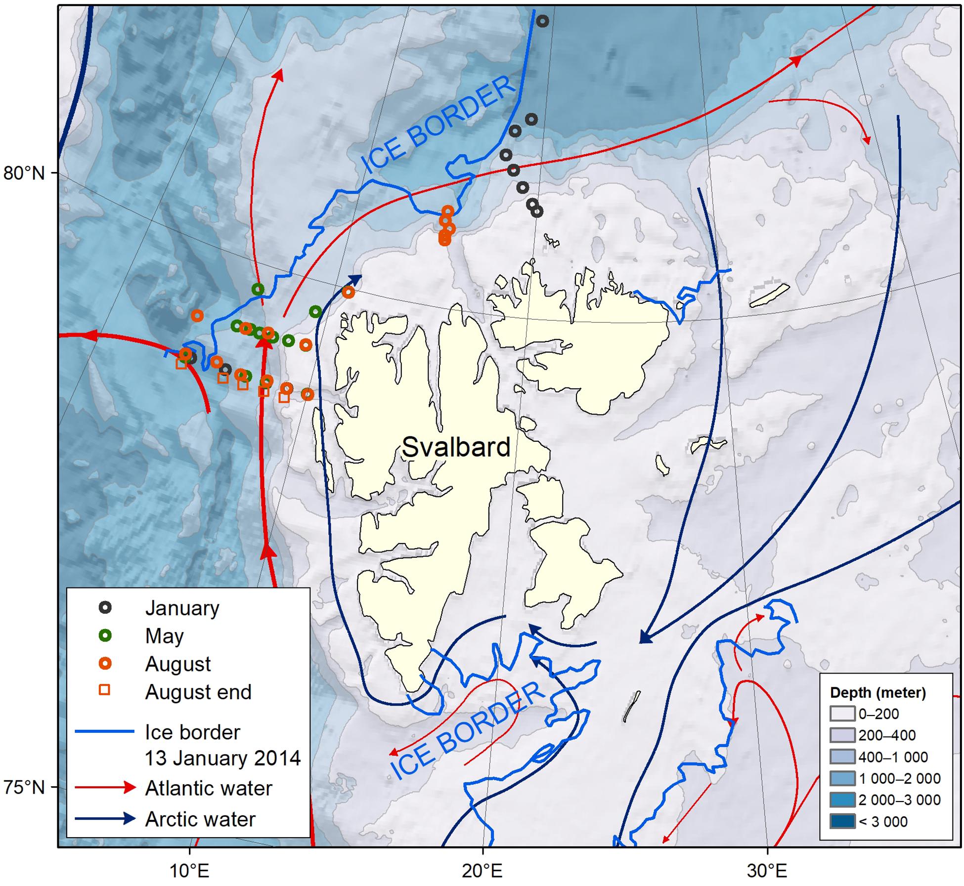
Figure 1. Map of the study area with station locations of the four different cruises. Shown are the major surface currents (Arctic in blue and the Atlantic water in red), and ice edge at 13th January 2014 (marked blue line).

FIGURE 2

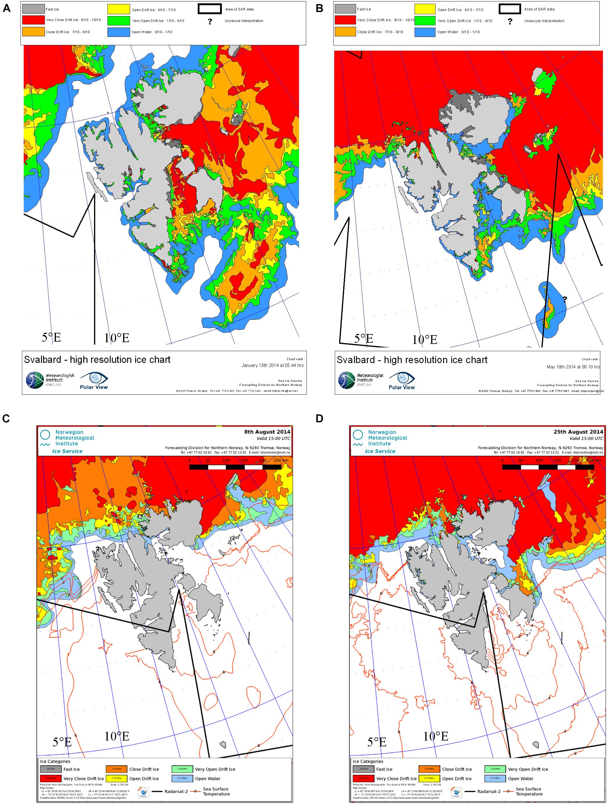
Figure 2. Sea ice cover around Svalbard for selected dates during the four cruises: (A) 13th of January, (B) 19th of May, (C) 8th of August, and (D) 25th of August in 2014. Data is obtained from the Ice Service of the Norwegian Meteorological Institute (MET, http://polarview.met.no/) and use their ice chart color scheme for very open drift ice (1–4/10ths), open drift ice (4–7/10ths), close drift ice (7–10/10ths), and fast ice (10/10ths).

Three different domains are defined based on the surface-water characteristics in January and on topography. The meltwater domain (MWD) includes the western and northern parts of the study area that are influenced by fresher surface water in spring and summer due to sea-ice melt from the sea ice formed the previous winter. The Atlantic core-water domain (AWD) is dominated by the AW and the shelf domain (SD) is located on the shelf near West Spitsbergen (Figure 1).

Materials and Methods

Sampling

The data of carbonate chemistry and inorganic nutrients were collected during four cruises in 2014 (Figure 1 and Supplementary Table S1). Three cruises were conducted as part of the CarbonBridge project (January, May, and August). A Fram Strait cruise was conducted in late August 2014, to obtain information on the Atlantic water inflow. The data analysis concentrates on two sections with the largest seasonal coverage on the eastern shelf of the Fram Strait (January, May, beginning of August and end of August) between ∼79–79.5°N and 4–10°E.

Water samples were collected from 8-L Niskin bottles mounted on a General Oceanics 12-bottle rosette equipped with a Conductivity-Temperature-Depth sensor system (CTD, Seabird SBE-911 plus). Water samples were collected at a total of 11 to 14 depths, from surface to 800 m depth (or at bottom) at each station, with the highest resolution in the upper 100 m. From these samples inorganic nutrients, nitrate (NO₃^–), phosphate (PO₄^3–), silicic acid [Si(OH)₄], and total DIC and total AT were determined.

Section figures and surface interpolation from weighted-gridding were performed in Ocean Data View software version 4.7 (Schlitzer, 2015).

Chemical Analyses

The DIC and AT were analyzed after the cruises at the Institute of Marine Research (IMR Tromsø, Norway) following the method described in Dickson et al. (2007). DIC was determined using gas extraction of acidified samples followed by coulometric titration and photometric detection using a Versatile Instrument for the Determination of Titration carbonate (VINDTA 3D, Marianda, Germany). The AT was determined by potentiometric titration with 0.1 N hydrochloric acid using a Versatile Instrument for the Determination of Titration Alkalinity (VINDTA 3S, Marianda, Germany). Routine analyses of Certified Reference Materials (CRM, provided by A. G. Dickson, Scripps Institution of Oceanography, United States) ensured the accuracy of the measurements, which was better than ±1 and ±2 μmol kg^–1 for DIC and AT, respectively.

Water samples for analysis of nutrients [NO₂^– + NO₃^–, Si(OH)₄, PO₄^3–] were frozen until post-cruise analysis by standard methods (Grasshoff et al., 2009) using a Flow Solution IV analyzer from O.I. Analytical, United States. The analyzer was calibrated using reference seawater from Ocean Scientific International Ltd., United Kingdom. Three replicates were analyzed for each sample. Note that we refer to the NO₃^– concentration throughout the study, but it is actually the sum of NO₂^– + NO₃^–, since NO₂^– levels are considered to be low in this area (Codispoti et al., 2005).

Calculations of the Carbonate System

We used AT, DIC, and nutrient concentrations as input parameters in a CO₂-chemical speciation model (CO2SYS program, Pierrot et al., 2006) to calculate other variables describing the carbonate chemistry, such as pH, fugacity of CO₂ (fCO₂), saturation state of calcium carbonate (Ω) for the two most common forms of aragonite (Ω_Ar) and calcite (Ω_Ca). The calculations are based on the carbonate system dissociation constants (K^∗1 and K^∗2) estimated by Mehrbach et al. (1973), modified by Dickson and Millero (1987) and the HSO₄^– dissociation constant from Dickson (1990).

Calcium carbonate (CaCO₃) saturation state (Ω) is commonly used to indicate a change in the CO₂ chemistry and the ocean acidification state, and indicates the dissolution potential for solid CaCO₃, such as calcareous shells and skeleton of marine organisms. When Ω < 1, solid CaCO₃ is chemically unstable and prone to dissolution (i.e., the waters are undersaturated with respect to the CaCO₃ mineral). In the Arctic Ocean, increased freshwater supply from sea-ice melt and river runoff have shown to decrease Ω (and provide a positive feedback on OA; Chierici and Fransson, 2009; Fransson et al., 2013, 2015). However, Ω is a chemical parameter showing the dissolution potential; most organisms require higher saturation state to grow due to the high energy demand of calcification. For example, the aragonite forming pteropod Limacina helicina, showed decreased calcification at Ω_Ar value of <1.4 and that lower values had negative effects on the shell density and thickness (e.g., Comeau et al., 2009; Lischka and Riebesell, 2012; Bednaršek et al., 2014).

Calculation of Seasonal Drivers of the Carbonate System

The strength of the effects and direction of different drivers of the change of DIC are schematically summarized in Figure 3. Earlier studies have shown that biological processes, such as photosynthesis and respiration explain much of the observed seasonal changes of the carbonate system in the Arctic Ocean as well as on the air-sea CO₂ exchange (Fransson et al., 2001, 2017; Chierici et al., 2011; Tynan et al., 2016). During photosynthesis, DIC and fCO₂ decrease, and pH and CaCO₃ saturation (Ω) increase. AT increases slightly during photosynthesis as a result of nitrate and hydrogen ion consumption when proteins are formed (Eq. 1a) but is less affected by photosynthesis than DIC (Figure 3). However, the AT change is twice as much as DIC during the production of calcium carbonate (Eq. 1b). This means that if CaCO₃ production occurs simultaneously with photosynthesis, both AT and DIC change, but if no CaCO₃ production takes place, only DIC changes. Thus, AT can give indications on the presence of CaCO₃-forming organisms and the contribution of CaCO₃ formation in sea ice. Sea-ice melting and formation cause changes to the carbonate chemistry where CaCO₃ is formed inside the ice (Assur, 1958) producing high CO₂-rich brine, which is rejected to underlying water (e.g., Rysgaard et al., 2007; 2013; Fransson et al., 2013, 2017). The solid CaCO₃ can be trapped in the ice until ice melting when it dissolves in the water (e.g., Rysgaard et al., 2012, 2013). The CO₂-rich brine is considered an important process for transport and sequestering of CO₂ in the Arctic Ocean to depth (e.g., Chierici, 1998; Fransson et al., 2013; Rysgaard et al., 2013). In our study area, sea ice is formed in the western part of the Fram Strait and in the area north of Svalbard while the AW inflow keeps the West Spitsbergen shelf ice free. Precipitation of CaCO₃ from the brine produces CO₂ (aq) and reduces AT in the brine (Eq. 1b), where Ca²⁺ and HCO₃^– denote the concentration of the calcium ions (Ca²⁺) and the bicarbonate ions (HCO₃^–) that are consumed as solid CaCO₃(s), CO₂, and water (H₂O) are produced.

FIGURE 3

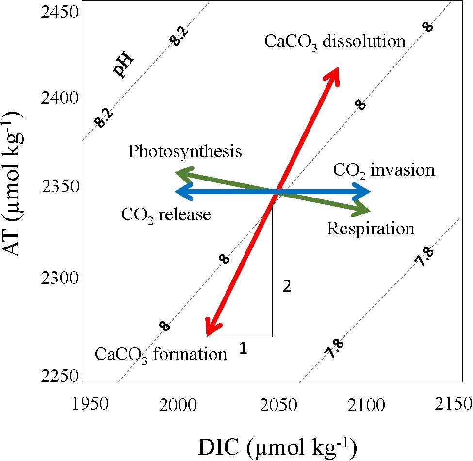
Figure 3. Effect of various processes driving the variability of dissolved inorganic carbon (DIC) and total alkalinity (AT), such as the photosynthesis/respiration (green arrow, DIC decrease/increase and a small AT increase/decrease); calcium carbonate formation/dissolution (red arrow, DIC reduces/increase by one and AT by two units); CO₂ invasion from atmosphere (blue arrow) increases DIC, and release of CO₂ to the atmosphere decreases DIC and AT stays constant in both cases. The dashed lines represent pH as a function of DIC and AT. The figure is adapted from Zeebe and Wolf-Gladrow (2001).

$2\mathrm{C}\mathrm{O}{}_2+\mathrm{NO}{}_3{}^{-}+\mathrm{H}{}^{+}+\mathrm{H}{}_2\mathrm{O}\to \mathrm{NHCH}{}_2\mathrm{CO}(\mathrm{org})+3.5\mathrm{O}{}_2(\mathrm{1a})$

$\mathrm{Ca}{}^2{}^{+}+2\mathrm{H}\mathrm{C}\mathrm{O}{}_3{}^{-}\to \mathrm{CaCO}{}_3(\mathrm{s})+\mathrm{H}{}_2\mathrm{O}+\mathrm{CO}{}_2(\mathrm{aq})(\mathrm{1b})$

Physical processes such as mixing of sub-surface water, usually high in CO₂ (low pH), play a large role for transferring CO₂ to the surface water, especially in fall due to increased wind-induced mixing and water column cooling. The DIC, fCO₂, and pH values also change with air-sea CO₂ exchange (C_EXCH). When the ocean fCO₂ is lower than the atmospheric, CO₂ is added to the water CO₂ (ocean sink, referred as invasion in Figure 3), and if ocean fCO₂ is higher, it loses CO₂ to the atmosphere during ocean outgassing (ocean CO₂ source, referred to as release in Figure 3). Since AT describes the ion-charge balance in the water, changes in the uncharged CO₂ will not affect AT (Figure 3). Seasonal warming and cooling affect the CO₂ solubility and explain part of the fCO₂ and pH variability.

The full inorganic carbonate system is used together with nutrient data from the seasonal cruises, to estimate the different components causing a change in DIC (C_DIC) from pre-bloom situation in January, to May, August to the end of August, described in Eqs 2–5. The January values of a salinity >35 in the upper 50 m were considered representative for concentrations before the onset of photosynthesis (Supplementary Table S2). In order to eliminate the change in concentrations due to salinity changes (i.e., dilution), all data were salinity-normalized to 35.1 (January salinity in the Atlantic water), after 35.1/S × C, where S refers to the observed salinity and C refers to the concentration of either DIC, AT, or NO₃. Since the area is considered to be nitrogen limited (Smith et al., 1987; Kattner and Becker, 1991; Randelhoff et al., 2018), we used the change in salinity-normalized nitrate concentrations from January to May/August (ΔNO₃, μmol kg^–1) converted to carbon using the carbon-to-nitrate (C:N) stoichiometric ratio based on 106:16 (Redfield et al., 1963), to estimate the biological component (C_BIO, mol C m^–2) of the total DIC change (C_DIC, mol C m^–2). Similar C:N ratios were found in the particulate organic matter during nitrogen consumption in May and August based on data collected in the same study (Paulsen et al., 2018). The difference between C_DIC, C_BIO, and C_CALC gives an estimate of the ocean’s role as an atmospheric CO₂ sink or source, C_EXCH (mol C m^–2) according to Eq. 5. C_BIO, C_EXCH, and C_CALC were integrated in the top 50 meters. This assumption was valid because that was the maximum depth of nitrate drawdown observed in Randelhoff et al. (2018). Following from the discussion above, the change in total alkalinity (ΔAT, mol C m^–2) corrected for the effect of photosynthesis by subtracting the NO₃^– change, was used to estimate the change in the calcification component of the C_DIC (mol C m^–2), referred to as C_CALC, mol C m^–2. The mean concentrations for each parameter in January at S > 35 were used to represent the pre-bloom state (Supplementary Table S2).

${\mathrm{C}}_{\text{DIC}}={\mathrm{C}}_{\text{BIO}}+{\mathrm{C}}_{\mathrm{EXCH}}+\mathrm{C}{}_{\text{CALC}}{}_{}(2)$

${\mathrm{C}}_{\text{BIO}}=\mathrm{\Delta }{\mathrm{NO}}_3\times \mathrm{C}:\mathrm{N}(3)$

${\mathrm{C}}_{\text{CALC}}=0.5(\mathrm{\Delta }\mathrm{AT}+\mathrm{\Delta }\mathrm{NO}{}_3)(4)$

${\mathrm{C}}_{\mathrm{EXCH}}={\mathrm{C}}_{\text{DIC}}-{\mathrm{C}}_{\text{BIO}}-\mathrm{C}{}_{\text{CALC}}{}_{}(5)$

Calculation of N^∗

The semi-conservative tracer N^∗ (μmol L^–1) allows us to easily identify high and low anomalies relative to the global mean concentration of fixed nitrogen lost relative to the phosphate concentration (PO₄^3–, μmol L^–1, Eq. 6). Deviations from conservative behavior are meaningful in identifying regions of denitrification and nitrogen fixation but only give indications for either nitrogen loss or replenishment, which are not always caused by nitrification. This means that negative (positive) values of N^∗ cannot be directly associated with denitrification (nitrogen fixation). The distribution and seasonal change in N^∗ in our study area was calculated using the relationship described in Eq. 6 (Deutsch et al., 2001). This relationship includes processes leading to deviations in the entire water column and not only in the euphotic zone as described in Gruber and Sarmiento (1997).

${\mathrm{N}}^{*}={\mathrm{NO}}_3-16\times {\mathrm{PO}}_4+2.9(6)$

In the equation, the constant 16 refers to the stoichiometric relationship between NO₃^– and PO₄^3– based on linear regression of world ocean nutrient data, and 2.9 is the constant derived by setting the global mean values to zero (Gruber and Sarmiento, 1997). The change in N^∗ reflects the net effect of denitrification and N₂ fixation, thus negative N^∗ values suggests a deficit of nitrogen relative to the global mean, whereas positive values denotes larger than the world mean thus suggesting a nitrogen excess possibly linked to nitrogen fixation. In this study N^∗ is used to study the seasonal change of the deficit or source that may be explained by denitrification or nitrogen fixation, but also by advection of waters of different N^∗.

Remotely Sensed Data

To obtain information on the timing and development of the phytoplankton bloom in our study area we used data on chlorophyll (Chl_sat) and particulate inorganic carbon (PIC, Figure 12) from the Moderate Resolution Imaging Spectroradiometer (MODIS) onboard Aqua spacecraft downloaded from NASA Goddard Space Flight Center, Ocean Ecology Laboratory, Ocean Biology Processing Group. Level 3, 8-day binned, 9 × 9 km resolution arrays were further sampled into grid cells limited by 1° longitude and 0.5° latitude (Børsheim et al., 2014).

Estimates of net primary production from the Vertically Generalized Production Model (VGPM, Behrenfeld and Falkowski, 1997) were downloaded from www.science.oregonstate.edu. Annual primary production was estimated by integrating the production time series from each grid cell throughout the productive season (Børsheim et al., 2014).

The information on sea-ice coverage for the Svalbard area during part of our field periods displayed in Figure 2 was obtained from ice charts of the Ice Service of the Norwegian Meteorological Institute (MET)¹ where the ice chart color scheme shows for very open drift ice (1–4/10ths), open drift ice (4–7/10ths), close drift ice (7–10/10ths), and fast ice (10/10ths).

Results

Seasonal Variability in the Atlantic Water Inflow and Shelf Water

Hydrography

Salinity and temperature in January, May, and August showed large variability between months (Figures 4–6). In January, there were clear longitudinal differences in the water-mass characteristics in the upper 100 m, which defined our study domains. At 4–5°E, there was a relatively thin surface layer in the upper 20 m, with lower salinity (<34.5) and temperature (<0°C) than in the surface water further to the east (Figures 4A,B). Between 5 and 8°E, the upper 100 m was more saline (>35) and warmer (4–6°C) than the other domains, while on the shelf (8–10°E) the salinity and temperature were intermediate, 34.8–35 and 2–4°C, respectively (Figures 4A,B). In January and May, a relatively warm (>2°C) water off shelf, with high salinity (>35), reached from >600 m depth to the surface. The warm (>4°C) core in the upper 150 m in January was not observed in May (Figures 4B, 5B). The low-salinity (<34.5) and cold water (<2°C) in January in the upper 50 m observed in the western part of the study area (3–5°E), was located further to the east, closer to the slope (5–8°E) in May (Figures 4–6). In August, this low-salinity upper-50 m layer had spread eastward to the slope and shelf, where increased temperature (>6°C) was observed, compared to in January and May (Figures 6A,B). The relatively low salinity and relatively high temperature contributed to a water stratification in the upper 50 m.

FIGURE 4

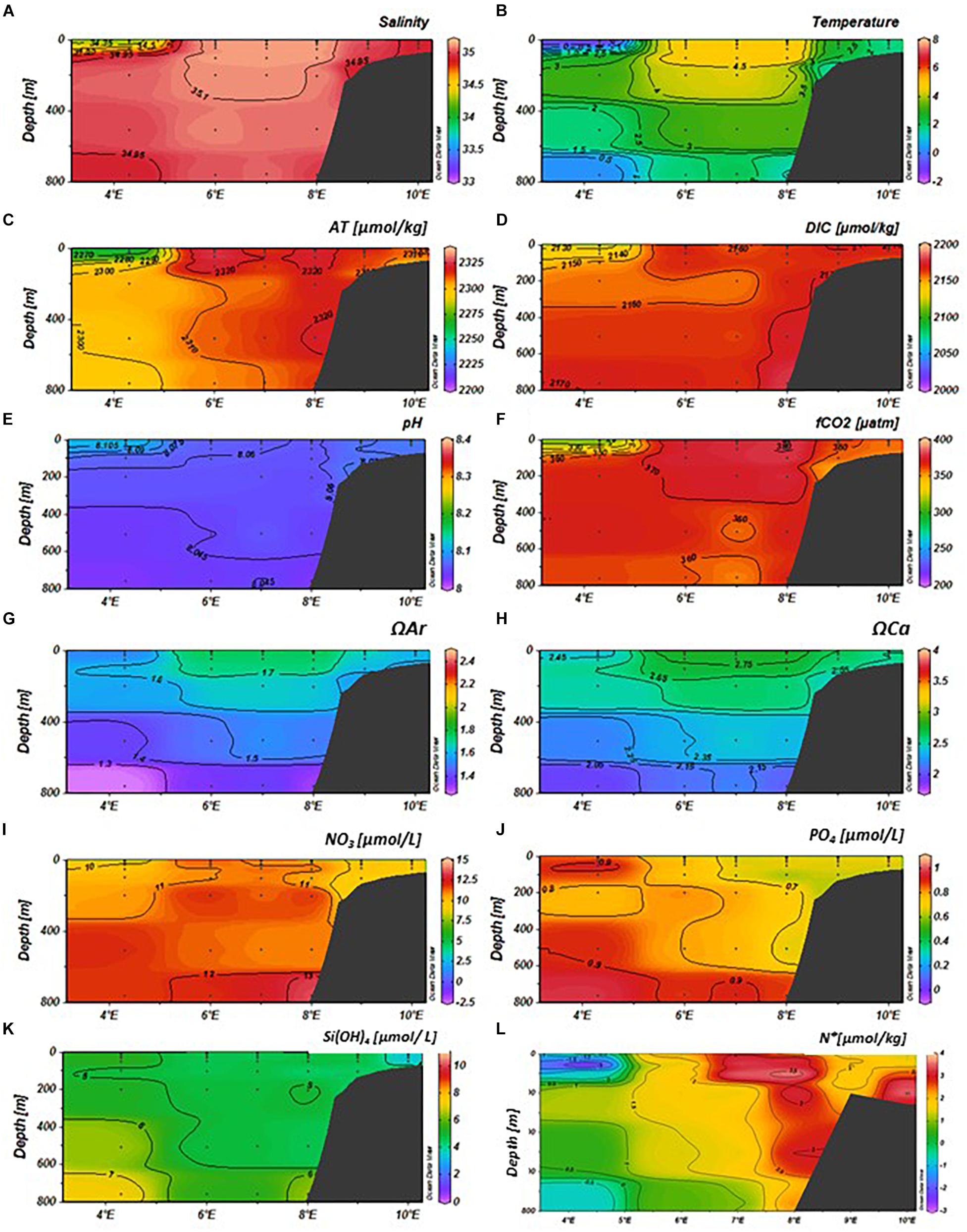
Figure 4. Variability of physical and chemical parameters in the eastern Fram Strait (latitude: 79–79.5°N, longitude: 4–10°E) in January 2014 from top; (A) salinity, (B) temperature (°C), (C) total alkalinity (AT, μmol kg^–1), (D) total dissolved inorganic carbon (DIC, μmol kg^–1), (E) pH, (F) fugacity of carbon dioxide (fCO₂, μatm), (G) aragonite saturation (ΩAr), (H) calcite saturation (ΩCa), (I) nitrate (NO₃, μmol L^–1), (J) phosphate (PO₄, μmol L^–1), (K) silicic acid (SiOH₄, μmol L^–1), and (L) N^∗ (μmol kg^–1, negative values denote denitrification, and positive values show nitrification). The sampling locations and depths are denoted as black dots. The section plot and interpolation were performed by the Ocean Data View program (Schlitzer, 2015).

FIGURE 5

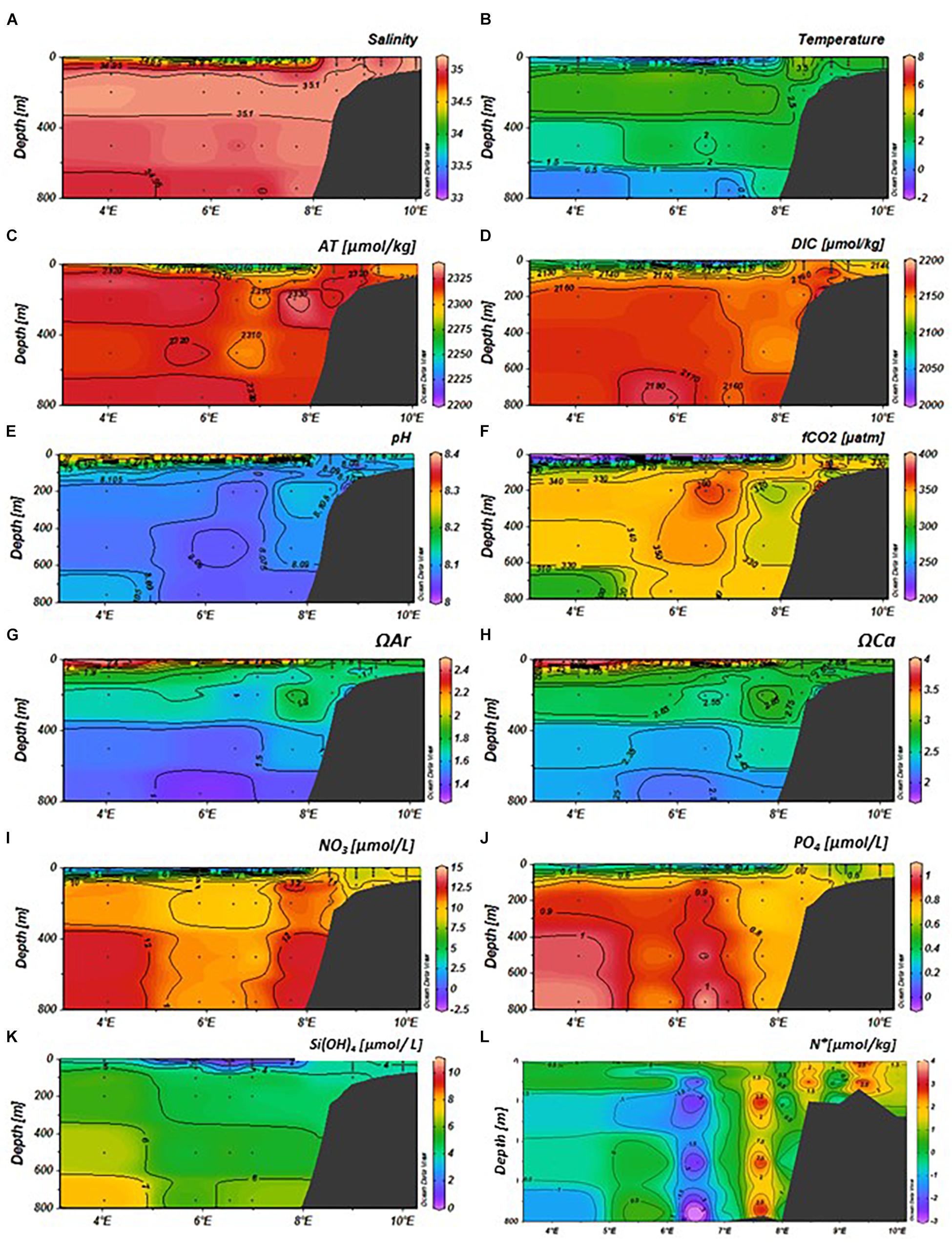
Figure 5. Variability of physical and chemical parameters in the eastern Fram Strait (latitude: 79–79.5°N, longitude: 4–10°E) in May 2014 from top; (A) salinity, (B) temperature (°C), (C) total alkalinity (AT, μmol kg⁻¹), (D) total dissolved inorganic carbon (DIC, μmol kg⁻¹), (E) pH, (F) fugacity of carbon dioxide (fCO₂, μatm), (G) aragonite saturation (ΩAr), (H) calcite saturation (ΩCa), (I) nitrate (NO₃, μmol L⁻¹), (J) phosphate (PO₄, μmol L⁻¹), (K) silicic acid (SiOH₄, μmol L⁻¹), and (L) N^∗ (μmol kg⁻¹, negative values denote denitrification, and positive values show nitrification). The sampling locations and depths are denoted as black dots. The section plot and interpolation were performed by the Ocean Data View program (Schlitzer, 2015).

FIGURE 6

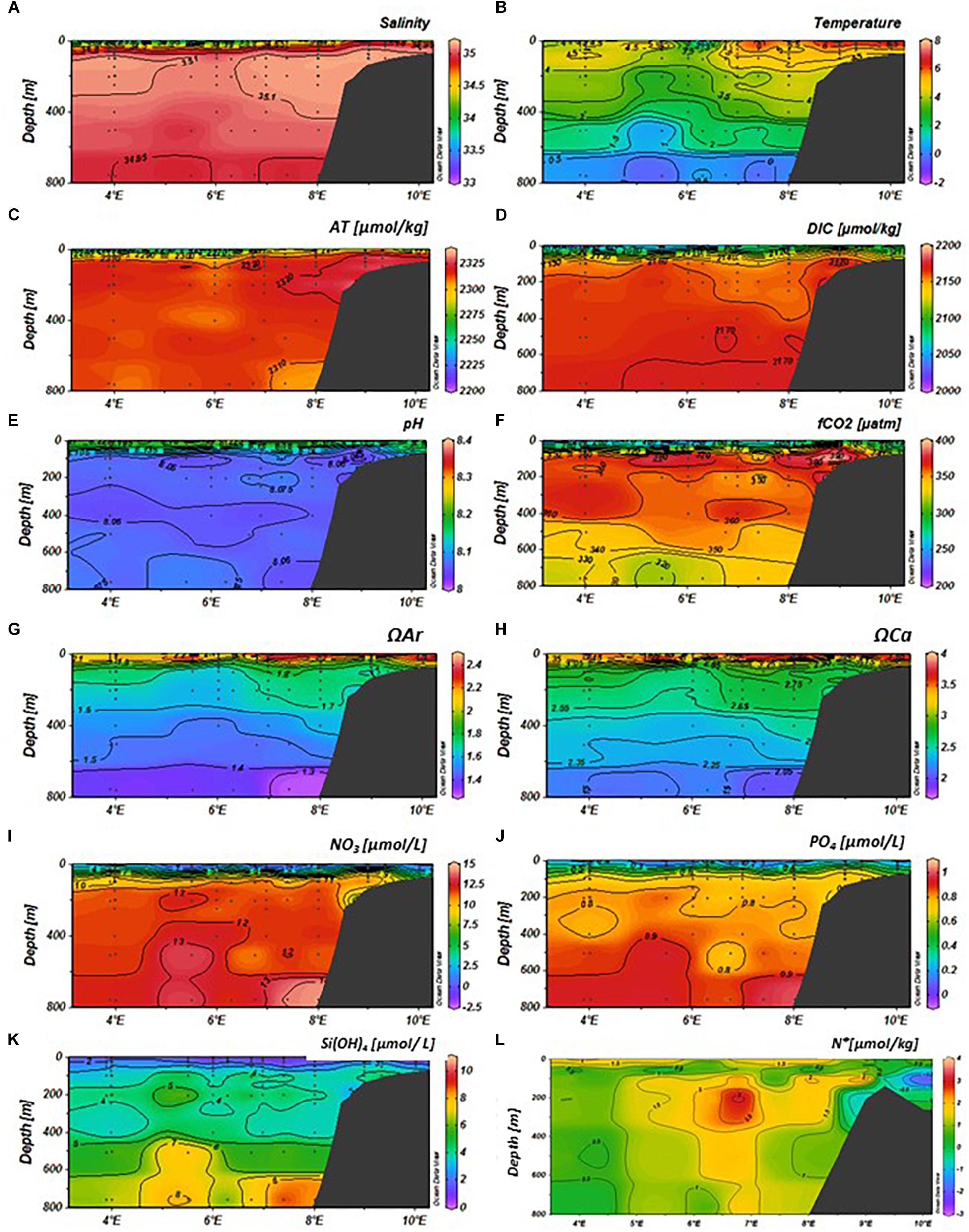
Figure 6. Variability of physical and chemical parameters in the eastern Fram Strait (latitude: 79–79.5°N, longitude: 4–10°E) in August 2014 from top; (A) salinity, (B) temperature (°C), (C) total alkalinity (AT, μmol kg⁻¹), (D) total dissolved inorganic carbon (DIC, μmol kg⁻¹), (E) pH, (F) fugacity of carbon dioxide (fCO₂, μatm), (G) aragonite saturation (ΩAr), (H) calcite saturation (ΩCa), (I) nitrate (NO₃, μmol L⁻¹), (J) phosphate (PO₄, μmol L⁻¹), (K) silicic acid (SiOH₄, μmol L⁻¹), and (L) N^∗ (μmol kg⁻¹, negative values denote denitrification, and positive values show nitrification). The sampling locations and depths are denoted as black dots. The section plot and interpolation were performed by the Ocean Data View program (Schlitzer, 2015).

Carbonate Chemistry and Ocean Acidification State

The AT, DIC, and fCO₂ values varied between the months. The AT values were lowest (about 2270 μmol kg^–1) in the upper 50 m at 4–5°E (MWD) in January (Figure 4C) and at 5–8°E (AWD) in May (Figure 5C), similar to the pattern observed in salinity (Figures 4A, 5A, 6A). The highest AT values of approximately 2325 μmol kg^–1 were observed in the locations of AWD and SD in the upper 50 m. In August, this low-alkalinity water was spread in the upper 50 m over the entire study area 4–10°E (Figure 6C), coinciding with low salinity (Figure 6A). The linear relationship between AT and salinity in the upper 50 m (AT = 57.07 × S + 315, R² = 0.95, N = 99), indicated a freshwater end-member of 315 μmol kg^–1. The DIC values in January and May were also low in the upper 50 m, coinciding with observations of low salinity and AT in the upper 50 m (Figures 4A,D, 5A,D). In August, the DIC trends were different than those observed in January and May, with the lowest DIC (<2100 μmol kg^–1), coinciding with both the lowest salinity and the highest temperature, in the upper 50 m (Figures 6A,B,D). At a few depths on the slope at 50–400 m depth, DIC was elevated compared to the same depth off the slope and on the shelf during all three cruises: in January (Figure 4D), May (Figure 5D) and August (Figure 6D). The fCO₂ values were undersaturated relative to the atmospheric fCO₂ levels of about 406 μatm (Fransson et al., 2017), with the lowest fCO₂ values in the upper 50 m in May (<200 μatm) and August (about 250 μatm), following a similar pattern to DIC (Figures 5D,F, 6D,F). In the water column on the shelf at about 9°E, the DIC and fCO₂ values were higher than the surrounding water. This was most evident in the fCO₂ that reached near atmospheric concentration of 406 μatm. The pH, Ω_Ar and Ω_Ca values also showed temporal variability, highest in May (Figures 5E,G,H) and August (Figures 6E,G,H) in the upper 50 m, coinciding with low DIC and fCO₂ values, in the stratified upper 50 m due to changes in salinity and temperature (Figures 5C,D, 6C,D). In May, the Ω_Ar and Ω_Ca values reached values up to a maximum of 2.5 and 4, respectively (Figures 5G,H), coinciding with low-salinity water (Figure 5A). The minimum Ω_Ar and Ω_Ca values of approximately 1.3 and 2.05, respectively, were observed at depths below 600 m in January (Figures 4G,H).

Nutrients, N^∗, and Chlorophyll

In the AWD, the water column had high concentrations of NO₃^–, PO₄^2–, and Si(OH)₄ in January throughout the water column with values of 11, 0.8, and 5 μM, respectively (Figures 4I–K). Interestingly, the PO₄^2– concentrations were higher near the ice edge (MWD) in the upper 200 m relative to the concentrations in AWD, whereas NO₃^– and SiOH₄ concentrations were lower in this region, relative to those in the AWD. In the upper 50 m, nutrient concentrations changed from relatively high (values) in January to depleted or near-depleted values in May (Figures 4, 6I–K). The Si(OH)₄ concentration had the largest decrease from January to May in the AWD, whereas PO₄^2– and NO₃^– concentrations showed largest decrease in the low-salinity water. This was where high pH and high Ω_Ar and Ω_Ca values were observed (Figures 5E,G,H). By August, Si(OH)₄ concentrations in the upper 50 m, were low (<2 μM) from off shore to the shelf (Figure 6K). The ratio between ΔNO₃ and ΔPO₄ over the period of maximum observed nutrient decrease (i.e., January to May), based on data in upper 50 m was 15.2 ± 0.5 μM, similar to the N:P ratio of 16 reported by Redfield et al. (1963).

In January, N^∗ values were generally positive, in excess of >3 μmol kg^–1 throughout the water column in the Atlantic-water influenced domain (Figure 4L). Similar values were also found on the shelf. Negative values of less than <−1 μmol kg^–1 were observed in the upper 100 m and below 650 m in the MWD (Figure 5L). By May, negative N^∗ remained in the MWD (Figure 5L). The most striking difference from January to May was the change of N^∗ in the western part of the AWD, which shifted from high positive N^∗ values in January, to negative values of less than −2 μmol kg^–1 at 7°E (Figure 5L). The change from positive to negative values were also observed on the slope (8°E), and on parts of the shelf at 9°E (Figure 5L). In August, the negative N^∗ values remained only in the intermediate water on the shelf, while the rest of the study area showed positive N^∗ values with a maximum of 2.8 μmol kg^–1 in the AWD (Figure 6L).

Remotely sensed chlorophyll data (Chl_sat) gives an overview of the succession of the phytoplankton bloom and clearly shows the onset of a bloom near the ice edge (Figures 7B,C, white areas show ice cover). In the first week of May (Figure 7A), the bloom increased around the ice edge (Figure 7C), continuing until late June (Figure 7D), when the Chl_sat decreased. At the end of July, Chl_sat increased again in our study area and persisted through August (Figures 7F,G) until the beginning of September after which the bloom ceased completely and reached undetectable values (Figure 7H). Largest values were observed in between May and mid-June (Figures 7B,C).

FIGURE 7

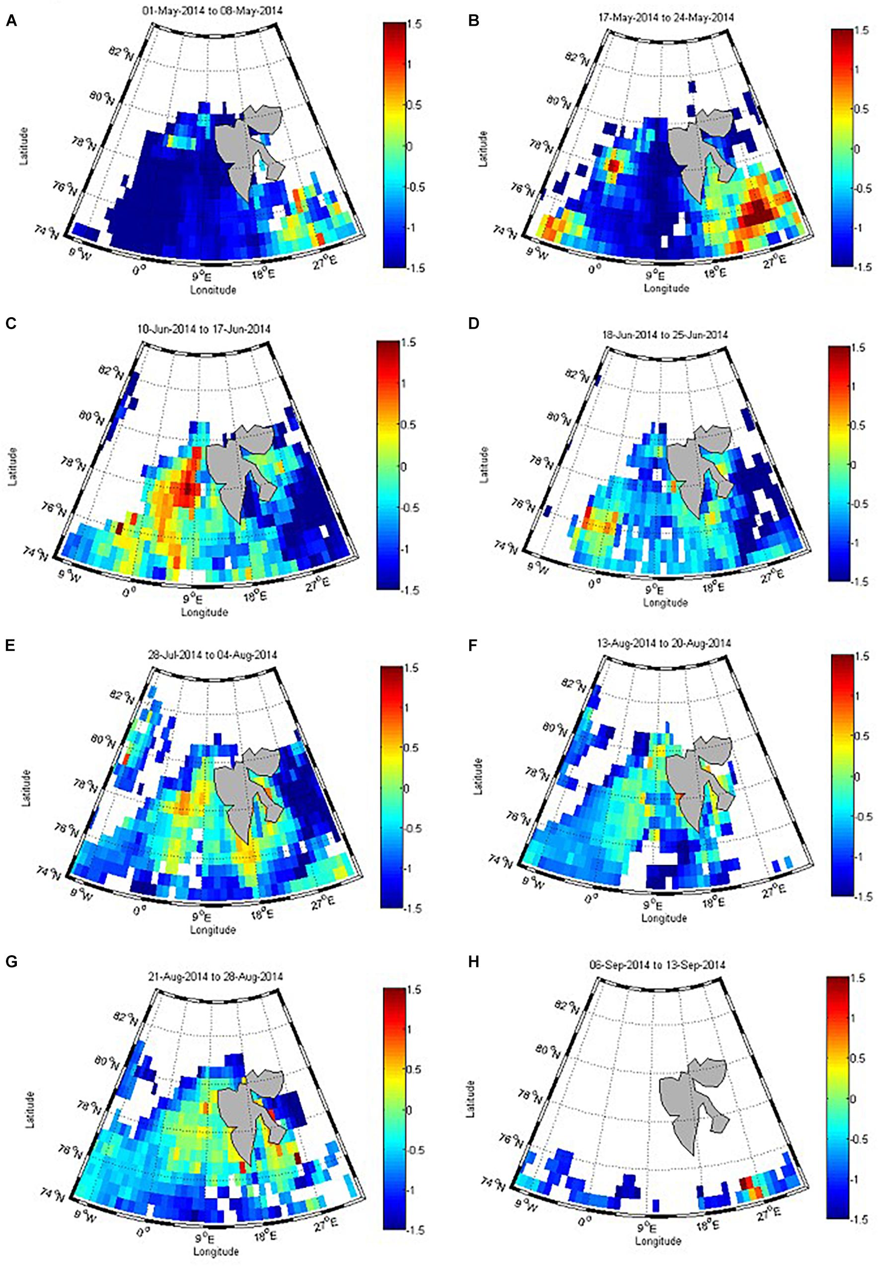
Figure 7. Remotely sensed chlorophyll a (Chl_sat, 8-day average) in May (A,B), June (C,D), July (E), August (F,G), and September (H), in 2014. Red values show the highest concentration and blue the lowest values on a logarithmic scale in mg m^–3.

Seasonal Drivers of DIC Change

Negative values of C_BIO signify loss of DIC in the surface water (i.e., CO₂) through net photosynthesis, whereas positive C_BIO values signify DIC release through net respiration. The C_BIO between January and May was between 1.9 and 2.2 mol C m^–2 (23–26 g C m^–2) in the MWD at about 4–6°E (Figure 8A). In the AWD, further east (>6 and 8°E) and along 79°N, the C_BIO averaged between −0.7 mol C m^–2 and near 0 mol C m^–2 at the shelf break (Figure 8A). On the West Spitsbergen shelf, C_BIO was −0.8 mol C m^–2. The C_BIO between January and August was −3.0 mol C m^–2 (−36 g C m^–2) in the AWD (Figure 8B), implying a 0.8 mol C m^–2 net community production in summer (between May and August).

FIGURE 8

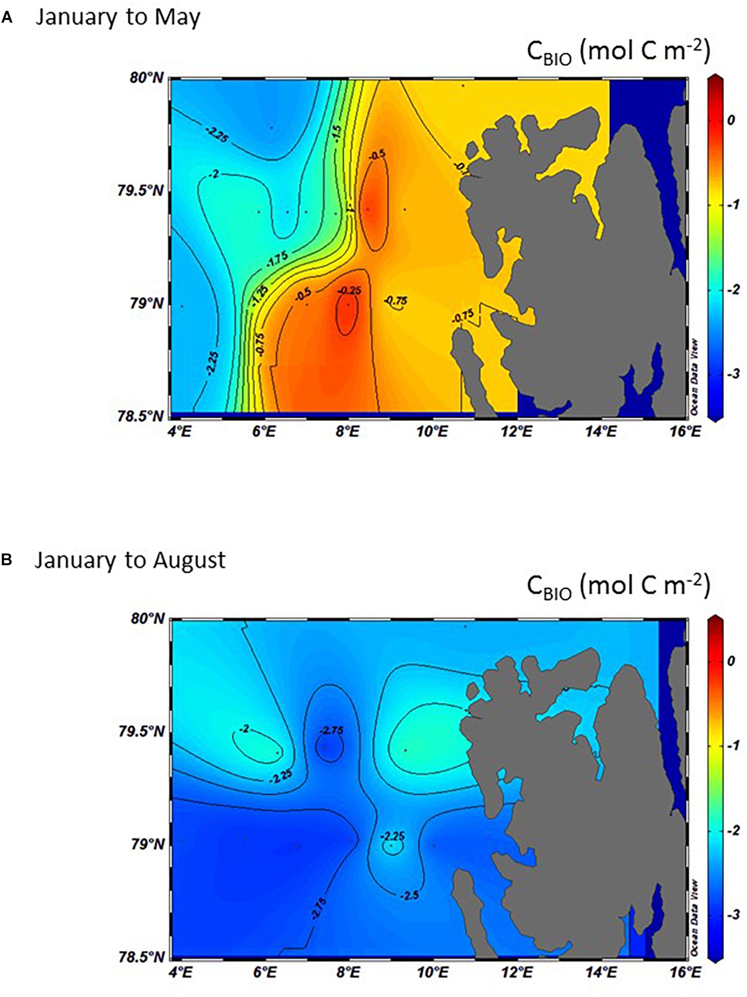
Figure 8. Interpolated and integrated C_BIO in the top 50 m (mol C m^–2) calculated from the difference between January and: (A) May and, (B) August in 2014. Negative numbers denote a loss of carbon through carbon consumption during phytoplankton production and a positive denote a gain of carbon during respiration and remineralization of organic matter.

Negative C_EXCH indicates an ocean loss, for example through CO₂ outgassing to the atmosphere (loss, negative values), while positive values denote an oceanic uptake of atmospheric CO₂ (Figure 9, Eq. 4). Between January and May, C_EXCH ranged from being a net oceanic CO₂ sink of about 0.5 mol C m^–2 on the SD, northern MWD and the northeast Svalbard, to become a net atmospheric CO₂ source (loss) between 0.5 and 0.2 mol C m^–2 in the southern MWD (Figure 9A). By August, the southern part of the study area (around 79°N), especially evident in the AWD, C_EXCH changed from an insignificant ocean CO₂ sink to a larger CO₂ sink of about 2.3 mol C m^–2 (Figure 9B). In the northern part, C_EXCH values were changed from a net sink to a net CO₂ source reaching a maximum release of 0.5 mol C m^–2. This was particularly pronounced in the area north of Svalbard (Figure 9B).

FIGURE 9

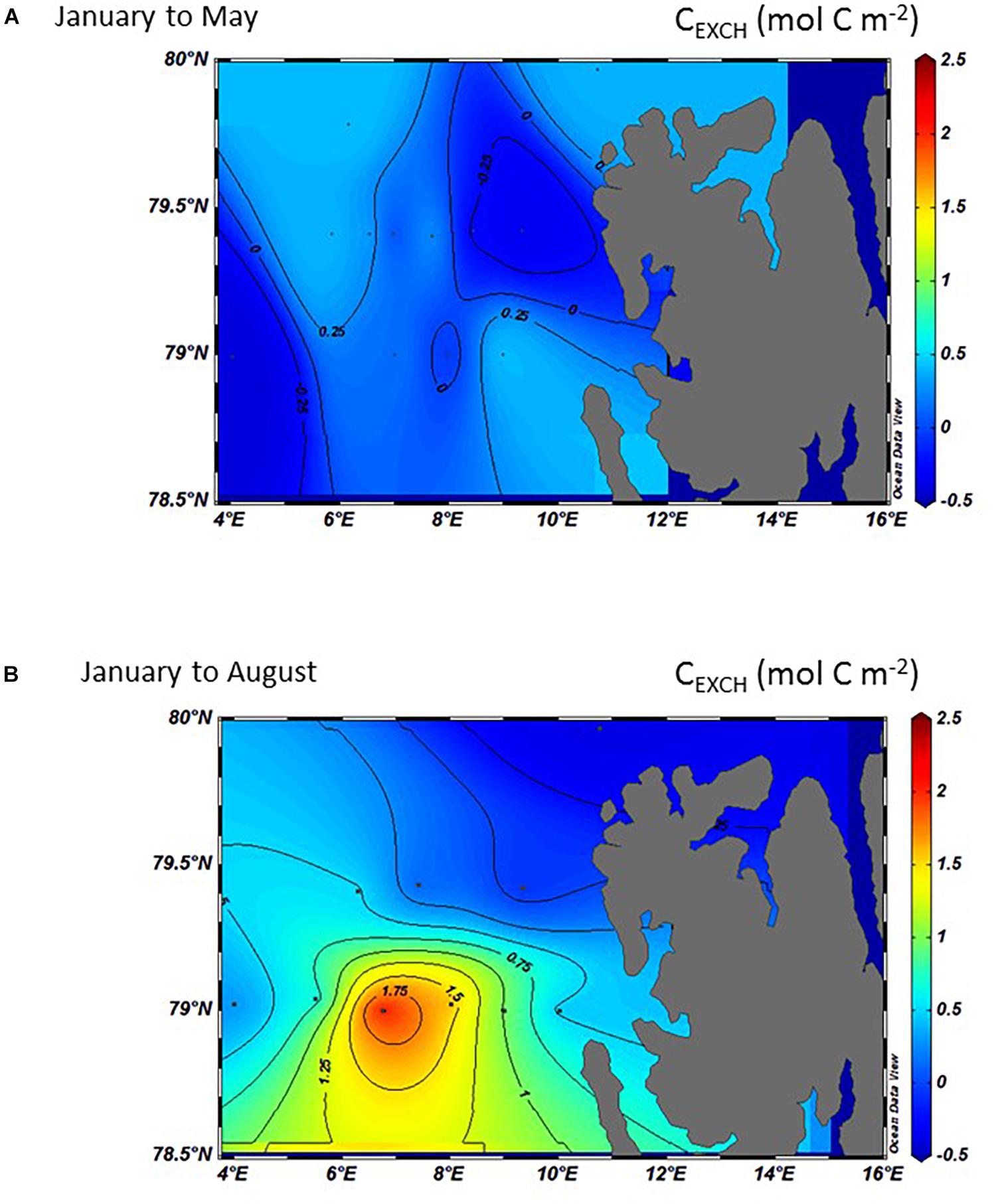
Figure 9. The interpolated and integrated C_EXCH in the top 50 meters (mol C m^–2) in 2014 calculated from the difference between January and: (A) May and, (B) August 2014. Negative numbers denote an ocean CO₂ sink from the environment, such as uptake from the atmosphere, and positive numbers denote an ocean CO₂ outgassing and source to the environment.

The influence of calcification or dissolution of CaCO₃ on the DIC change (C_CALC) was investigated following Eq. 4, where positive values signify a gain in DIC through CaCO₃ dissolution and negative values a loss through CaCO₃ formation/precipitation. Equation 4 is based on the salinity-normalized AT, corrected for photosynthesis using the nitrate change. Since AT is not affected by air-sea CO₂ exchange, it is only CaCO₃ dissolution that explains the increase in AT and ultimately the increase in C_CALC. Generally, the area showed a DIC gain (positive C_CALC) for the whole region, except for the small loss of 0.1 mol C m^–2 found in the SD between January and May (Figure 10A). At this time, the largest DIC gain of up to 0.5 mol C m^–2 was found in the MWD and the lowest DIC gain of less than 0.10 mol C m^–2 in the area north of Svalbard (Figure 10A). In the AWD, the largest C_CALC values were 0.3 mol C m^–2. Between January and August, the DIC gain derived from C_CALC had generally increased throughout the study area except in the MWD and north of Svalbard compared to the change between January and May. The largest DIC gain derived from C_CALC was observed in the AWD to a maximum of 0.7 mol C m^–2 between January and August, hence an increase between May and August of about 0.4 mol C m^–2 (Figure 10B).

FIGURE 10

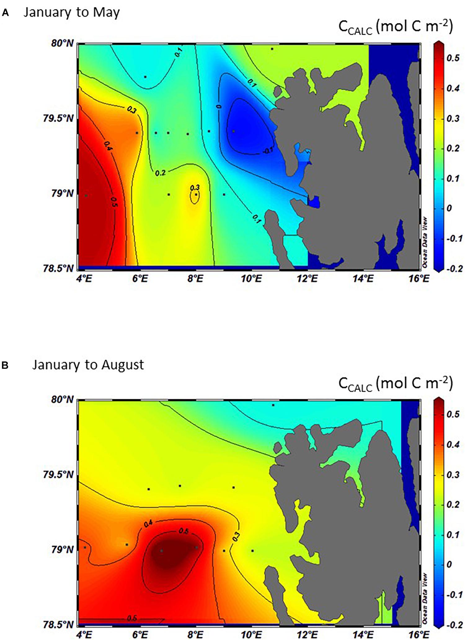
Figure 10. The interpolated and integrated C_CALC in the top 50 meters (mol C m^–2) in 2014 calculated from the difference between January and: (A) May and, (B) August 2014. Positive values denote a gain in DIC through CaCO₃ dissolution and negative values a loss through formation of CaCO₃.

Figure 11 shows a composite of the seasonal change of C_BIO, C_EXCH, and C_CALC focusing on variability of the area between 79–79.5°N and 4–10°E between January and May (Figure 11A), May and August (difference in the DIC between January and August, Figure 11B), and between beginning August and the end of August (Figure 11C). Figure 11 clearly shows a large biological DIC uptake, C_BIO in the MWD between January and May (Figure 11A). C_BIO DIC uptake increased (more negative C_BIO) in the SD and AWD from May to August to a maximum C_BIO DIC change of −3.0 mol C m^–2 (Figure 11B). By the end of August, C_BIO showed a net DIC gain in the AWD and MWD of up to 2.3 mol C m^–2, sustaining biological DIC uptake (negative C_BIO) in part of the MWD and SD of about 0.2 mol C m^–2 (Figure 11C). Between January and May, C_EXCH showed that the ocean generally acted as a small net oceanic sink of atmospheric CO₂ of about 0.4 mol C m^–2 (Figure 11A). By beginning of August, the CO₂ sink increased in the AWD of up to 2.3 mol C m^–2 (Figure 11B). At the end of August, the CO₂ sink decreased greatly and changed C_EXCH by −3.8 mol C m^–2 from a sink to become a CO₂ source, releasing CO₂ to the atmosphere in the AWD (Figure 11C). In January to May and May to August, throughout the study area, the C_CALC resulted in a DIC gain of maximum of 0.5 mol C m^–2 in the MWD in January to May (Figures 11A,B). In the SD, C_CALC showed less importance than the other domains (Figures 11A–C). By the end of August, the C_CALC changed from a DIC gain to a DIC loss (Figure 11C) of a maximum of about −0.5 mol C m^–2.

FIGURE 11

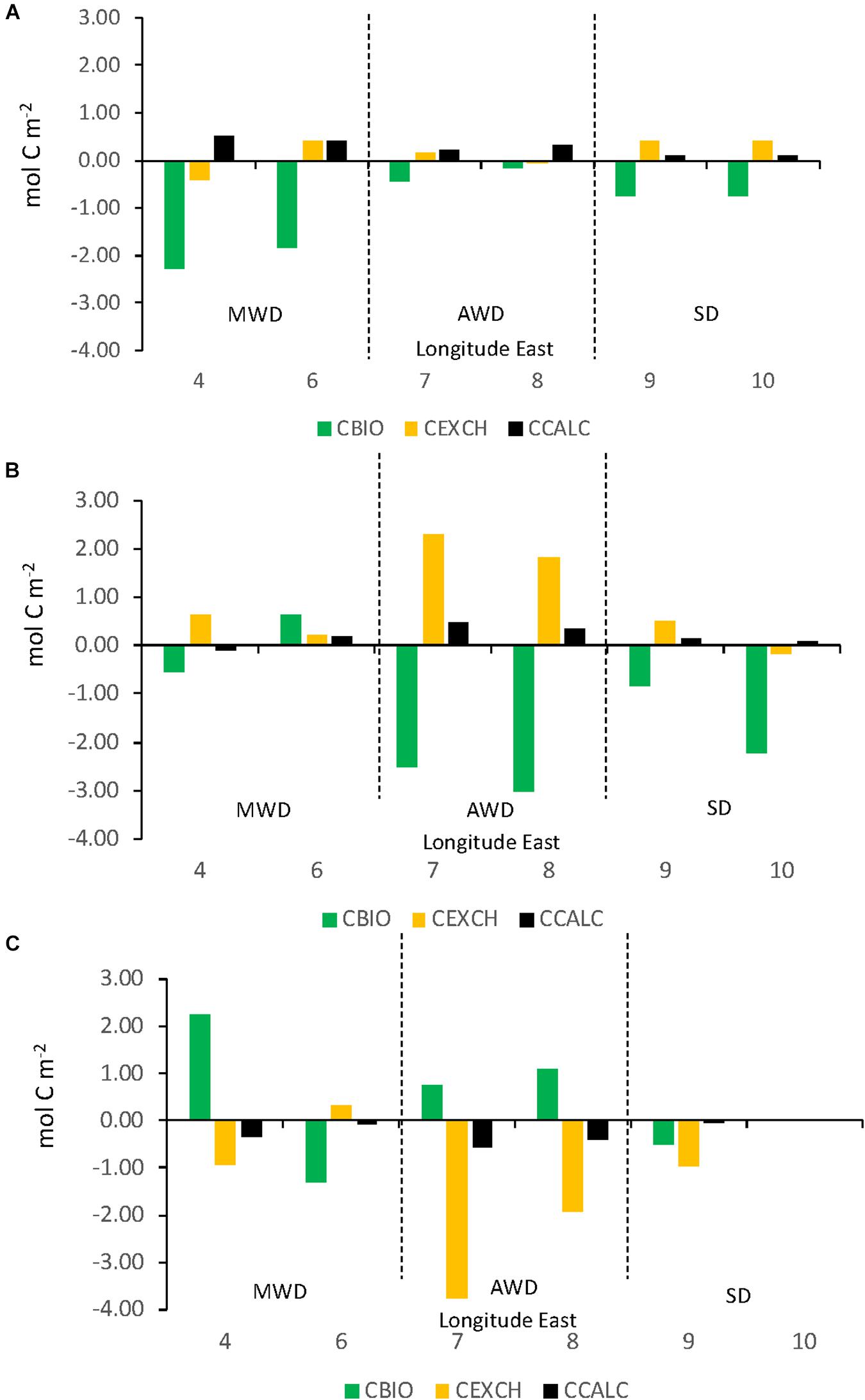
Figure 11. The integrated change of C_BIO (green columns), C_EXCH (orange columns), and C_CALC (black columns) in top 50 meters (y-axis, mol C m^–2) between: (A) January and May, (B) May to August, and (C) August to end of August along the 79°N section in eastern Fram Strait (x-axis Longitude°E). The dashed vertical lines divide the section in the three domains; meltwater domain (MWD), the Atlantic water domain (AWD), and the shelf domain (SD). Positive numbers denote a gain of carbon, and negative denote a loss of carbon.

The large C_CALC values in May and August were found in the area influenced by sea-ice formation and melt, such as in the MWD in May, and in the AWD in August. In our study area and time of year, the remotely sensed data on particulate inorganic carbon (PIC_sat) showed a clear seasonal trend (based on data in the area 78.5–79.5°N and 4–10°E) from values less than 0.1 μmol kg^–1 in May to maximum PIC values of up to 0.6 μmol kg^–1 in August (Figure 12). The seasonal trend agrees with our C_CALC estimates for the AWD, but the values are too low to explain the C_CALC in the AWD of up to 0.5 mol C m^–2 between May and August (Figure 11B). Part of the difference between the PIC_sat and C_CALC are based on the methodological difference. The C_CALC values are integrated to 50 m and PIC_sat values are based on the surface ocean.

FIGURE 12

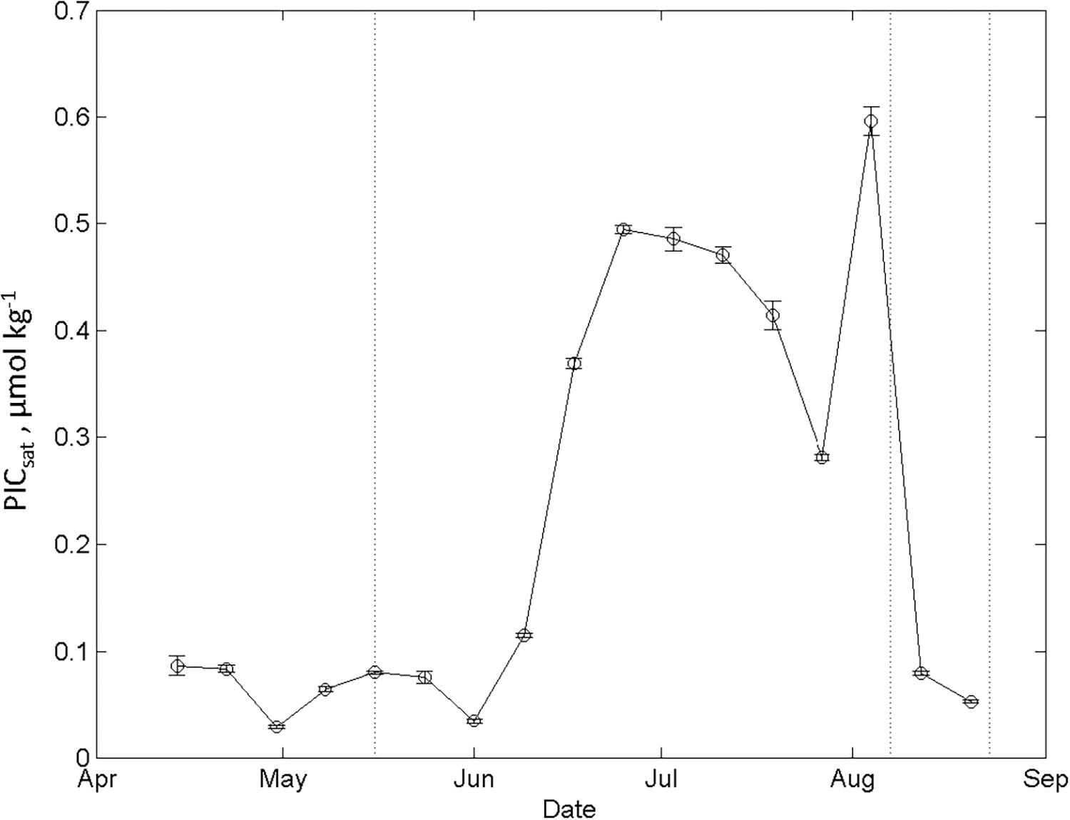
Figure 12. The seasonal evolution of the remotely sensed particulate inorganic carbon (PIC_sat, μmol kg^–1) from mid-April to end of August 2014, in the area between longitude 4 and 10°E, and latitude between 78.5 and 79.5°N.

The succession of C_BIO from May to end of August was also observed from the remotely sensed chlorophyll data (chl_sat). The maximum 8-day mean values of chl_sat in the area 79.75–78.75°N shown by longitude reached >0.5 mg m^–3 (in the MWD) by 23rd April and reached the highest values of 6 mg m^–3 in the beginning of July at 6°E (Figure 13A). After the peak, chl_sat rapidly decreased to reach values below 1 mg m^–3 (Figure 13A). The succession of the bloom was also investigated in the three domains, where chl_sat > 0.5 mg m^–3 was observed one week later in the AWD and SD domains than in MWD, on the 1st May (Figures 13B,C). In the AWD, the chl_sat varied between 3 and 1.5 mg m^–3 throughout the season and showed less seasonal variability than the other domains (Figure 13B). In the shelf domain at 9°E, generally higher chl_sat of about 3 mg m^–3 was observed than on the shallow shelf at 10°E, where chl_sat values steadily increased and reached the highest values of 1.7 mg m^–3 by the 23rd August. One week later, chl_sat values rapidly declined to undetectable values (Figure 13C). The chl_sat in the MWD clearly showed a spring bloom between end of April to end of May, followed by a secondary bloom from mid-June to end of July (Figure 3A).

FIGURE 13

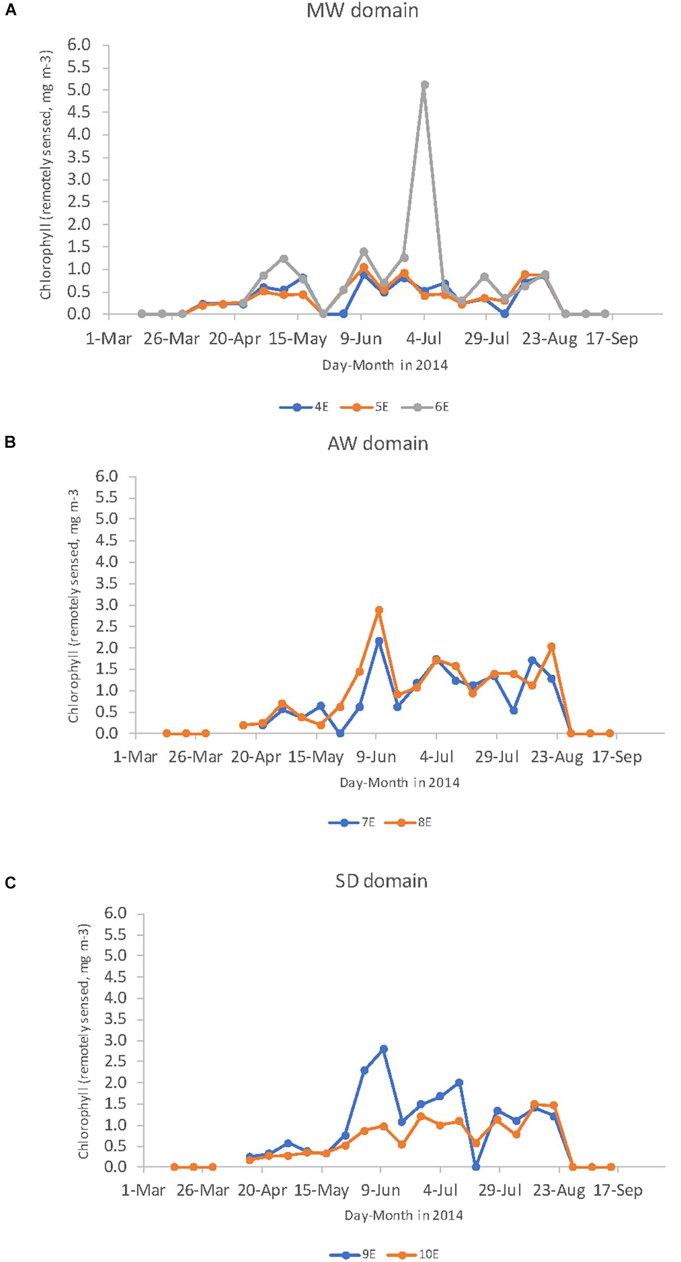
Figure 13. The seasonal variability of the maximum value of remotely sensed chlorophyll a (mg m^–3) in the area between 79.75 and 78.75°N from 4 to 10°E divided in the: (A) meltwater influenced domain (MWD), (B) the Atlantic water domain (AWD), and (C) in the shelf domain (SD) from 4th of February to 12th of October in 2014. Values are Level 3, 8-day binned, 9 × 9 km resolution arrays from the Moderate Resolution Imaging Spectroradiometer (MODIS) onboard Aqua spacecraft downloaded from NASA Goddard Space Flight Center, Ocean Ecology Laboratory, Ocean Biology Processing Group.

Discussion

Succession of the Bloom and Variability in Primary Productivity Estimates

Our study agrees with several studies that show evidence of extensive spring blooms near the ice edge in the Arctic Ocean and its shelf seas. These blooms are mainly caused by relatively high-light conditions, meltwater-induced stratification and high nutrient availability, controlled by the nitrate concentration (i.e., Sakshaug, 2004; Wassmann and Reigstad, 2011; Assmy et al., 2017). Randelhoff et al. (2018) found an overall increase in ammonium values from May to August, explained by the remineralization after the spring bloom when the plankton community shifted toward a nutrient-recycling state during summer. Later in summer these authors suggested that thermal convection added nutrients and likely CO₂-rich sub-surface water to the surface ocean. Increased remineralization (where C_BIO results in increased DIC) and mixing at the end of the summer would explain the rapidly changing conditions from a net biological DIC consumption and ocean CO₂ sink in August to a net biological DIC source in late August (Figure 11C). Increased mixing of CO₂-rich sub-surface water would also explain the change in C_EXCH from an ocean CO₂ sink area in August to atmospheric CO₂ release by the end of August. Our study supports these findings: the spring bloom started near the ice edge in the west and moved eastward as the season progressed with most of the biological DIC consumption estimated in the AW domain and on the shelf (SD; Figure 11).

Based on the difference between January and May (2.2 mol C m^–2 and 26 g C m^–2) and between January and August (3.0 mol C m^–2 and 36 g C m^–2) estimates (Figure 8 and Table 1), about 75% of the C_BIO occurred in spring, whereas the remaining 25% (0.8 mol C m^–2 and ∼9 g C m^–2) occurred in summer (between May and August). This spring value is similar to the annual export production estimates of 28–32 g C m^–2 in the Barents Sea presented by Fransson et al. (2001) using a similar approach as in our study. Our C_BIO estimates are based on the loss of NO₃^–, sometimes referred to as new production, and do not consider production based on recycled nitrogen, other than nitrate (Muggli and Smith, 1993). In the Labrador Sea, primary production showed a similar bloom succession as in our area, with high nitrate-based spring bloom in May and recycled production in August (Tremblay et al., 2006). They estimated the ratio between the relative contribution of NO₃^– to total nitrogen uptake ratio, the f-ratio, to be 0.8 in May and 0.2 in August (Tremblay et al., 2006). The f-ratios from their study was used to convert our C_BIO estimates to total production based on all nitrogen sources (C_BIOTOT). This resulted in a C_BIOTOT of up to 2.6 mol C m^–2 for the spring bloom (between January and May), 1.4 mol C m^–2 in summer (between May and August), and a total annual C_BIOTOT of 4.0 mol C m^–2.

TABLE 1

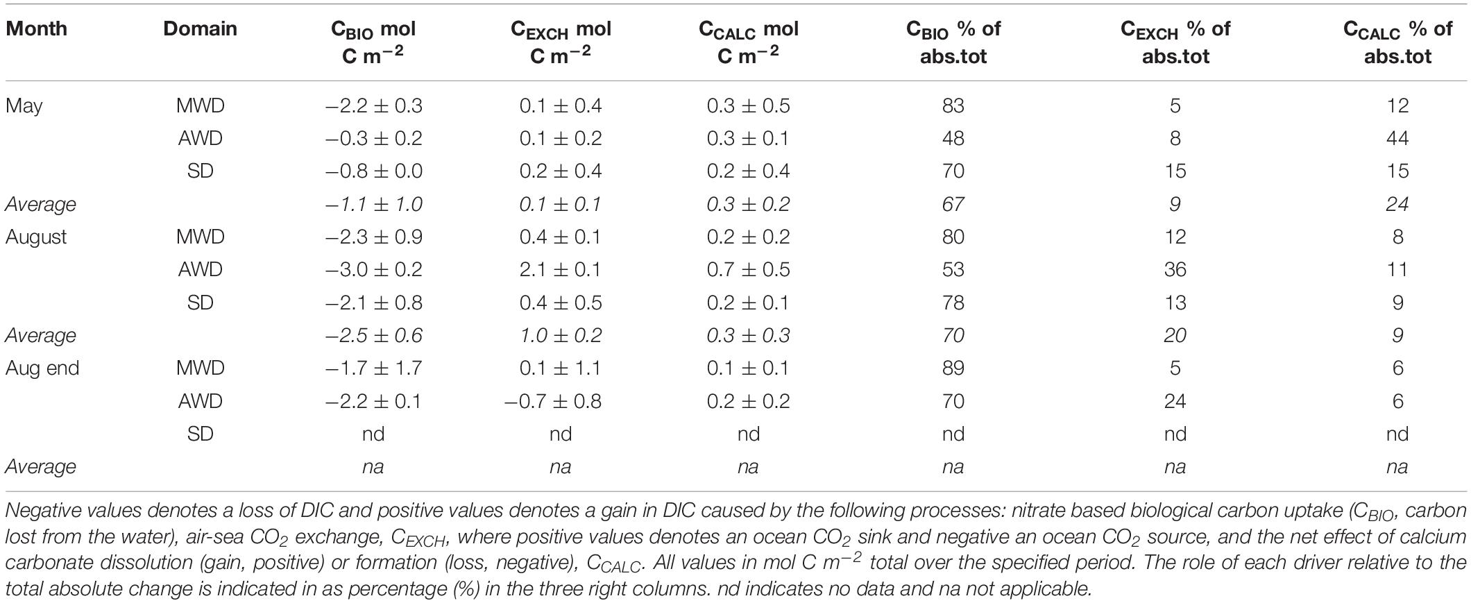
Table 1. Summary and direction of the estimated drivers of the mean and standard deviation for the seasonal DIC change (C_DIC, mol C m^–2) integrated in the top 50 meters in the three study domains: meltwater influenced domain, MWD, Atlantic water domain, AWD, and the shelf domain, SD, in May, August, and end of August 2014.

Based on chl_sat data, the onset of the bloom occurred close to the 1st of May, resulting in a daily C_BIO estimate of 0.10 and 0.14 mol C m^–2 d^–1, or 1.2 to 1.7 g C m^–2 d^–1 using data collected between 16th and 23th of May (equivalent to 16 to 23 “bloom days,” Figure 13). The daily total production estimate (C_BIOTOT) for May range between 0.11 and 0.16 mol C m^–2 d^–1 (1.4–2.0 g C m^–2 d^–1). Sanz-Martín et al. (2018) estimated total production (Gross Primary Production, GPP) west and north of Svalbard in May 2014. They used oxygen (O₂) production in incubations with water collected from the spring-bloom conditions. Their study estimated a daily GPP of about 6.2 μmol O₂ l^–1 d^–1 (converted to 4.8 μmol C l^–1 d^–1 by C:O ratio of 106:138) from northwest Svalbard shelf stations (P1 and P5, Supplementary Table S1). Converting their value to the same bloom period as ours, integrated to 50 m results in a daily estimate of 0.24 mol C m^–2 (2.9 g C m^–2 d^–1) which is larger than our daily C_BIOTOT estimates from 0.11 to 0.16 mol C m^–2 d^–1 b (2.6 mol C m^–2 for 16–23 days). This is likely due to the integration of their value to 50 m, which probably overestimates the Sanz-Martín et al. (2018) GPP value. Wassmann et al. (2010) presented model estimates of GPP in the area west of Svalbard between 74 and 80°N, where they found a maximum annual GPP of 120 g C m^–2 (10 mol C m^–2), with an annual mean of 75 g C m^–2 (6.3 mol C m^–2).

In the open ocean north of Svalbard, Assmy et al. (2017) estimated a biological carbon consumption based on ¹⁴C uptake during the spring bloom of 1.3 mol C m^–2, integrated in the top 50 m for 27 days, between 25th of May and 22nd of June. In the same area and time, Fransson et al. (2017) used a similar method as in our study (nitrate-deficit method) and estimated a biological DIC consumption integrated in the top 50 m during the spring bloom of 1.6 mol C m^–2 in May–June. Both the estimates of Assmy et al. (2017) and Fransson et al. (2017) are lower than our C_BIO estimates of 2.2 mol C m^–2 in May, suggesting that the eastern Fram Strait region has larger net community production than the basin north of Svalbard, in spring.

Estimated remotely-sensed biological carbon consumption NCP_sat in our study area showed an annual net production up to 1.3 mol C m^–2 (Figure 14). Part of the difference between the NCP_sat and the C_BIO estimates of 3.0 mol C m^–2 (36 g C m^–2) for the full period between January and August was likely caused by methodological considerations. A difference in the integration depth can be expected, NCP_sat was based on a surface chlorophyll a and PAR values, and variable euphotic zone depth, likely shallower than the 50-meter C_BIO estimate. For example, Randelhoff et al. (2018) measured a mixed layer depth of 10–15 m at the ice edge.

FIGURE 14

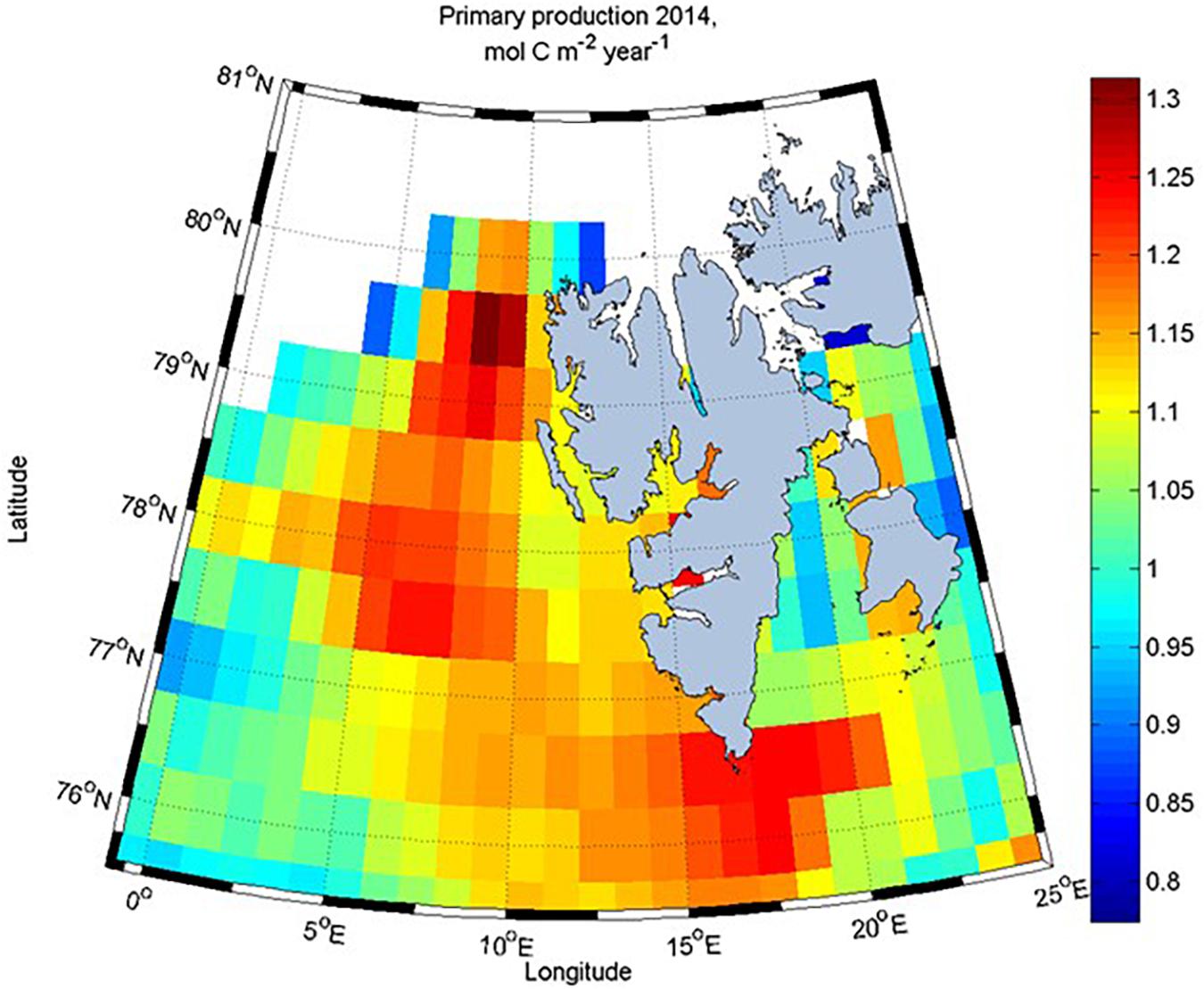
Figure 14. Remotely sensed net primary production (NCP_sat, mol C m^–2) for 2014 from the Vertically Generalized Production Model (VGPM, Behrenfeld and Falkowski, 1997) downloaded from www.science.oregonstate.edu. NCP_sat was estimated by integrating the production time series from each grid cell throughout the productive season (Børsheim et al., 2014).

Dissolved inorganic carbon uptake by Arctic productivity is similar to Antarctic estimates. In the Atlantic sector of the Southern Ocean in the Weddell Sea, Hoppema et al. (2007) estimated the NCP using integrated nutrient-deficiency methods such as in our study, and estimated NCP (same as our C_BIO) to be 1.5 mol C m^–2 for a 4-month period between November and March 2005 (Hoppema et al., 2002). Extrapolated values to include the entire marginal ice zone, resulted in much larger NCP estimates of up to 4.1 mol C m^–2 in the same area (Smith and Nelson, 1990).

In summary, there is a large variability in primary productivity estimates for polar regions, including our area of study, based on environmental and methodological considerations at different time and spatial scales. The C_BIOTOT estimates are about half the maximum values from O₂ incubations and a third of the model estimates (both GPP), but twice as large as the primary production estimates based on ¹⁴C by Assmy et al. (2017), the nitrate-deficit values of Fransson et al. (2017) and the NCP_sat from this study. Seasonally, up to 75% of the net community productivity is constrained to the spring bloom. Areas west of Svalbard present twice as much annual production than in the Arctic, north of Svalbard. Finally, the depth of integration and the length of the sampling period can bias estimates in regions with shallow, and variable, mixed layer depth. Our analysis, encompassing from winter to autumn, highlights the importance of the seasonal signal in this high-latitude region.

The Oceanic Sink of Atmospheric CO₂ in Fram Strait Area and Its Variability

Several studies estimating the air-sea CO₂ fluxes and the annual net CO₂ sink show that the Arctic Ocean, the Fram Strait and waters around Svalbard act as atmospheric CO₂ sinks (e.g., Tynan et al., 2016; Yasunaka et al., 2016, 2018; Fransson et al., 2017). The 18-year annual average of observed seawater fCO₂ and a self-organizing mapping technique showed that the Arctic Ocean acted as an ocean CO₂ sink between 8 and 12 mmol m^–2 d^–1 and a daily mean in a full annual cycle of 5 mmol m^–2 d^–1 (Yasunaka et al., 2018). In our estimates, the study area showed a small oceanic CO₂ sink until May at an average of 0.12 ± 0.06 mol C m^–2 for the period January to May. By August, the ocean CO₂ uptake increased to a large net ocean CO₂ sink of an average of 1.1 ± 1.0 mol C m^–2 and a maximum CO₂ sink of 2.1 mol C m^–2 (25 g C m^–2) in the AWD for the January to August period (Table 1). This suggests a mean daily ocean CO₂ uptake of 10 mmol m^–2 d^–1 and a maximum of 21 mmol m^–2 d^–1 in August (100 days). By the end of August, the AWD shifted to a significant CO₂ source of about 0.7 mol C m^–2 (Table 1). Accounting for the study period between January and August, this results in an ocean net annual CO₂ sink between 4 and 8 mmol m^–2 d^–1, which are similar to the results by Yasunaka et al. (2018). The winter-to-summer ocean CO₂ uptake estimates of 3.7 mol C m^–2 (44 g C m^–2) by Fransson et al. (2001) in the Barents Sea in the upper 50 m, are nearly twice as large as our maximum estimate of 2.1 mol C m^–2 (25 g C m^–2). Their relatively large CO₂ uptake were mainly driven by biological DIC uptake in the biologically productive waters of the Barents Sea. Model estimates for the Barents Sea showed an annual oceanic CO₂ uptake between 10 and 40 g C m^–2, related to warm and cold years (Slagstad and Wassmann, 1996), which were similar to our estimates of the annual net oceanic CO₂ uptake between 10 and 25 g C m^–2 for the whole period from January to May and August. In the Greenland Sea, the ocean acted as a CO₂ sink throughout the year of about 53 g C m^–2 (Anderson et al., 2000). On the other hand, our estimate is much larger than the Atlantic water influenced Kara-Laptev Sea of 1 g C m^–2 (Fransson et al., 2001). In the southern Beaufort Sea, surface waters were undersaturated with respect to atmospheric CO₂ throughout the year and constituted a net sink of 14 g C m^–2 (1.2 mol C m^–2 yr^–1), with ice coverage and ice formation limiting the CO₂ uptake during winter (Shadwick et al., 2011a). They explained that the CO₂ uptake was largely driven by under-ice and open−water biological activity, with high subsequent export of organic matter to the deeper water column. These results emphasize the large regional variability of the annual net oceanic sink of atmospheric CO₂ and the importance to consider the local processes driving the exchange.

In the high-latitude Southern Ocean, Fransson et al. (2004) used a similar method as in our study, i.e., winter-to-summer deficits of nitrate in several regions, such as the polar front (APF), winter ice edge (WIE), and the seasonal ice edge (SIE). In the SIE and the APF, a net ocean release of CO₂ to the atmosphere of 0.1–0.5 mol m^–2, respectively, was calculated over a time scale of several months (from austral winter to January). In the WIE, the ocean acted as a net atmospheric CO₂ sink of about 0.1 mol m^–2, which is similar to our values for the MWD for the period January to May (Table 1).

Dissolution and Sources of CaCO₃

Increased C_CALC suggests dissolution of CaCO₃, which may be caused by breakdown of CaCO₃ shells and skeleton from calcifying organisms or dissolution of ikaite minerals from sea ice melt water (Rysgaard et al., 2012, 2013; Fransson et al., 2013). Our estimate of C_CALC showed that the corresponding DIC change due to calcification or dissolution, was less significant than the C_BIO but at times similar to the values of C_EXCH (Figure 11 and Table 1). We found that the large C_CALC values in May were either found in the area influenced by sea ice formation and melt such as in MWD, or in the AWD domain in August.

The shells (coccoliths) affects the reflectance of the surface water and results in a turquoise milky surface which is clearly observed using remotely sensed sensors (Tyrrell et al., 1999). In our study area and time of year, the remotely sensed data on particulate inorganic carbon (PIC_sat) showed a clear seasonal trend from values less than 0.1 μmol kg^–1 in May to maximum PIC values of up to 0.6 μmol kg^–1 in August (Figure 12). The seasonal PIC_sat trend agrees with our C_CALC estimates for the AWD but as previously stated, the values are too low to explain the DIC gain through CaCO₃ dissolution estimated from C_CALC of maximum of 0.3 and 0.7 mol C m^–2 in May and August, respectively (Table 1). Calcifying phytoplankton blooms are known to occur after the spring bloom and may sustain growth in relatively nutrient depleted waters during summer. This is observed on the Arctic inflow shelves such as the Bering Sea and Barents Sea and very common in the North Atlantic (e.g., Robertson et al., 1994), but not common in the Arctic Ocean (i.e., Tyrrell and Merico, 2004 and references therein). The low PIC_sat during our study agreed with observations of very low cell numbers of calcifying phytoplankton observed during the CarbonBridge study (Egge et al., 2018). Perhaps these shells were not locally formed and dissolved but transported from the south with the Atlantic water inflow or from the West Spitsbergen fjords (e.g., Lalande et al., 2016). This was the explanation for the E. huxleyi blooms, the most common and opportunistic calcifying phytoplankton, that was observed in the upper 50 m of the marginal ice zone in the Barents Sea in August 2003 (Hegseth and Sundfjord, 2008). These blooms were attributed to intrusions of Atlantic water bringing cells of oceanic phytoplankton species via the subsurface circumpolar boundary current west of Svalbard and then eastward along the Eurasian Shelf break.

Another possible source for DIC gain through CaCO₃ dissolution is the dissolution of ikaite particles (which is a form of CaCO₃ formed in sea ice) that has been recently released from melting sea ice and dissolved in the upper water column. Sea-ice cover will obstruct remotely sensed observations of ikaite and is most likely not included in the PIC_sat values (Figure 12). Consequently, sea-ice derived ikaite could explain the relatively high DIC gain from C_CALC of about 0.3 mol C m^–2 estimated between January and May. This implies that most of the C_CALC increase of about 0.4 mol C m^–2 (from 0.3 to 0.7 mol C m^–2; Table 1) in the AWD between May and August is attributed to dissolution of advected CaCO₃ shells (Table 1). By the end of August, the C_CALC values are the lowest throughout the study area (Table 1), agreeing well with the drastic decrease in PIC_sat values (Figure 12).

The Role of Nitrogen Fixation and Denitrification Based on N^∗

N^∗ values from our study varied with season and ranged between −3 and +2.5 μmol kg^–1, which is the same range as reported from other ocean basins (Gruber and Sarmiento, 1997). The high values (>1 μmol kg^–1) in the AWD is generally found in well-oxygenated waters, such as in the North Atlantic >35°N (Gruber and Sarmiento, 1997). Consequently, the high N^∗ in the eastern Fram Strait may be enriched by the inflowing Atlantic waters and does not necessarily imply a local source due to on-site N₂ fixation. To estimate the different nitrogen sources and sinks requires information on the isotopic nitrogen ratios (Granger et al., 2011). Sipler et al. (2017) estimated the depth-integrated N₂ fixation in the ice-free season (June to September) west of Svalbard and the Barents Sea to about 1.5 g N m^–2 in the upper 50 m. In the Nansen Basin, north of Svalbard, integrated N₂-fixation was significantly lower and between 0 and 0.5 g N m^–2 (Sipler et al., 2017).

The negative N^∗ values observed on the shelf slope and in shelf bottom water, especially evident in August, may indicate a nitrogen loss due to benthic denitrification (Figure 6L). This was observed to be the case in the Pacific Arctic inflow region, in the eastern Bering Sea shelf where benthic denitrification caused a nitrogen loss of between 2 and 13 μmol L^–1 in April 2007 and 2008 (Granger et al., 2011). This implies that modifications such as increased nitrogen loss on the Bering Sea shelf may decrease the nitrogen concentrations in the Pacific water inflow waters and the surface water column in the Arctic Ocean (e.g., Jones et al., 2003). The Arctic outflow water exits through the Fram Strait, mainly in the East Greenland Current along the Greenland shelf (e.g., de Steur et al., 2014). It is unlikely that the negative N^∗ values observed in the water column in January and May in the MWD was caused by Pacific water outflow. Denitrification has also been found in melting Arctic sea ice before the under-ice spring bloom oxygenates the surface water (Rysgaard et al., 2008). This could explain the nitrogen loss in the upper water column in January as well as the increasing N^∗ values in the surface water as the bloom progressed and oxygenated the water from May to August (Figures 4L, 5L, 6L). However, sea-ice processes cannot explain the negative N^∗ values before May in the deeper parts of the water column (>200 m). The decreased N^∗ from January to May below 200 m depth for whole area, may be caused by contribution of another water mass. About half of the AW transported by the WSC, recirculated between 76 and 81°N, exits the Fram Strait from the north, and has modified the chemical and physical properties of AW (MAW; Rudels et al., 2000; Marnela et al., 2013). According to Sipler et al. (2017), N₂ fixation was much lower in the Arctic Ocean than in the AW inflow area. Consequently, one explanation for the decreased N^∗ between January and May could be that the AW looses nitrogen as it resides in the low N₂ fixation area further north and during its return to the Fram Strait contains less nitrogen as well as less heat. By August, the nitrogen increased by 2 μmol L^–1, showing a nitrogen gain, which implies a larger contribution of original AW. The strength and magnitude of the recirculation of MAW in the Fram Strait show large interannual variability (Rudels et al., 2000; de Steur et al., 2014). Moreover, observations and models show that eddy activity results in substantial seasonal and spatial variability in the recirculation and facilitates subduction of AW (Hattermann et al., 2016).

Conclusion and Future Outlook

Phytoplankton DIC uptake (C_BIO) played by far the most important role for the observed DIC change throughout the study area and explained up to 89% of the total DIC change. The C_EXCH played a minor to moderate role and was most significant in August in the Atlantic water domain, explaining about 36% of the relative importance of the DIC drivers. In May, dissolution of sea-ice derived CaCO₃ (ikaite) played a moderate but important role to explain the net effect of the DIC gain in all domains. By August, the biological DIC uptake (C_BIO) had increased in all domains, and at this time we observed the largest C_EXCH gain, and continuing gain from CaCO₃ dissolution, most likely from an advected source. Of the total DIC gain between January and August (sum of C_EXCH and C_CALC ∼2.8 mol C m^–2, Table 1), 25% was explained by CaCO₃ dissolution and the remaining 75% of C_EXCH was due to ocean CO₂ uptake from the atmosphere as a result of the high biological CO₂ demand during photosynthesis between May and August.

In a future scenario, decreased sea ice and more open water exposed to atmosphere will facilitate direct ocean CO₂ uptake through increased air-sea CO₂ flux as long as the surface water is undersaturated in CO₂ relative to the atmospheric CO₂ level. In contrast, less sea-ice associated CaCO₃ dissolution (ikaite) will decrease the addition of total alkalinity, thus the buffering capacity against acidic input (e.g., CO₂), decreasing the CO₂ uptake potential in spring. However, with the influence of advected CaCO₃ shells later in summer, the buffering potential could be fully or partly restored but at a later stage. Moreover, less influence of melting sea ice may potentially decrease nitrate removal caused by denitrification. A larger inflow of well-oxygenated Atlantic water will also result in lower potential for denitrification to take place. Several studies show that increased CO₂ concentrations enhance primary production in spring in this area (Holding et al., 2015; Sanz-Martín et al., 2018), which would allow larger DIC uptake through biological CO₂ consumption. In that case, progressing ocean acidification in the surface water would be mitigated fully or partly by biological CO₂ consumption. In a scenario of increased advection of Atlantic water, this buffer may become more important for the CO₂ uptake capacity and on-going ocean acidification. However, the net effect of the studied processes on the DIC change and ocean CO₂ uptake in the Arctic inflow region will ultimately depend on a combination of several processes such as changes in primary production, stratification, nutrient availability, the net carbon export out of the mixed layer, as well as changes in the advection of warm Atlantic water. Warming of the surface ocean will decrease the ocean CO₂ uptake solubility due to decreased CO₂ dissolution in warmer compared to colder water. With less meltwater in spring, the sea-ice ikaite contribution to the surface water would decrease, hence having consequences for the ocean to act as a net CO₂ sink in future. Furthermore, the increase in wind-induced vertical mixing due to increased open water in winter could contribute to increased DIC in the surface water, perhaps resulting in a CO₂ source.

Data Availability

The datasets generated for this study are available on request to the corresponding author.

Author Contributions

MC, AF, and MV involved in the sampling and study design. MC performed the data analyses, and created the tables and figures. MC completed the writing of the manuscript with contributions from MV and AF. MV contributed with the calculations. KB contributed with the calculations based on the remotely sensed data. MC and AF collected and analyzed the carbonate chemistry.

Funding

This study is a contribution to the Carbon Bridge (RCN-226415) project funded by the Norwegian Research Council and the Flagship Research Program “Ocean acidification and effects in Northern waters” within the FRAM-High North Research Centre for Climate and Environment (MC and AF).

Conflict of Interest Statement

The authors declare that the research was conducted in the absence of any commercial or financial relationships that could be construed as a potential conflict of interest.

Acknowledgments

We are grateful for the splendid support by the captain and crew on the two research vessels RV Helmer Hanssen and RV Lance.

Supplementary Material

The Supplementary Material for this article can be found online at: https://www.frontiersin.org/articles/10.3389/fmars.2019.00528/full#supplementary-material

Footnotes

1. ^ http://polarview.met.no/

References

ACIA (2005). Arctic Climate Impact Assessment. ACIA Overview Report. Cambridge: Cambridge University Press.

Google Scholar

AMAP (2013). AMAP Assessment 2013: Arctic Ocean Acidification. Oslo: Arctic Monitoring and Assessment Programme.

Google Scholar

AMAP (2018). Arctic Ocean Acidification. Tromsø: Arctic Monitoring and Assessment Programme.

Google Scholar

Anderson, L. G., Drange, H., Chierici, M., Fransson, A., Johannessen, T., Skjelvan, I., et al. (2000). Annual carbon fluxes in the upper Greenland Sea based on measurements and a box-model approach. Tellus B Chem. Phys. Meteorol. 52, 1013–1024. doi: 10.1034/j.1600-0889.2000.d01-9.x

CrossRef Full Text | Google Scholar

Anderson, L. G., Ek, J., Ericson, Y., Humborg, C., Semiletov, I., Sundbom, M., et al. (2017). Export of calcium carbonate corrosive waters from the East Siberian Sea. Biogeosciences 14, 1811–1823. doi: 10.5194/bg-14-1811-2017

CrossRef Full Text | Google Scholar

Anderson, L. G., Olsson, K., and Chierici, M. (1998). A carbon budget for the Arctic Ocean. Glob. Biogeochem. Cycles. 12, 455–465. doi: 10.1029/98gb01372

CrossRef Full Text | Google Scholar

Årthun, M., Eldevik, T., Smedsrud, L. H., Skagseth, Ø, and Ingvaldsen, R. B. (2012). Quantifying the influence of Atlantic heat on Barents Sea ice variability and retreat. J. Clim. 25, 4736–4743. doi: 10.1175/jcli-d-11-00466.1

CrossRef Full Text | Google Scholar

Assmy, P., Fernández-Méndez, M., Duarte, P., Meyer, A., Randelhoff, A., Mundy, C. J., et al. (2017). Leads in Arctic pack ice enable early phytoplankton blooms below snow-covered sea ice. Sci. Rep. 7:40850. doi: 10.1038/srep40850

PubMed Abstract | CrossRef Full Text | Google Scholar

Assur, A. (1958). Composition of sea ice and its tensile strength in Arctic Sea Ice. Natl. Acad. Sci. Nat. Res. Counc. 598, 106–138.

Google Scholar

Bednaršek, N., Tarling, G. A., Bakker, D. C. E., Fielding, S., and Feely, R. A. (2014). Dissolution dominating calcification process in polar pteropods close to the point of aragonite undersaturation. PLoS One 9:e109183. doi: 10.1371/journal.pone.0109183

PubMed Abstract | CrossRef Full Text | Google Scholar

Behrenfeld, M. J., and Falkowski, P. G. (1997). Photosynthetic rates derived from satellite-based chlorophyll concentration. Limnol. Oceanogr. 42, 1–20. doi: 10.4319/lo.1997.42.1.0001

CrossRef Full Text | Google Scholar

Beszczynska-Möller, A., Fahrbach, E., Schauer, U., and Hansen, E. (2012). Variability in Atlantic water temperature and transport at the entrance to the Arctic Ocean. 1997–2010. ICES J. Mar. Sci. 69, 852–863. doi: 10.1093/icesjms/fss056

CrossRef Full Text | Google Scholar

Børsheim, K. Y., Milutinović, S., and Drinkwater, K. F. (2014). TOC and satellite-sensed chlorophyll and primary production at the Arctic Front in the Nordic Seas. J. Mar. Syst. 139, 373–382. doi: 10.1016/j.jmarsys.2014.07.012

CrossRef Full Text | Google Scholar

Carmack, E., Polyakov, I., Padman, L., Fer, I., Hunke, E., Hutchings, J., et al. (2015). Toward quantifying the increasing role of oceanic heat in sea ice loss in the new Arctic. Bull. Am. Meteorol. Soc. 96, 2079–2105. doi: 10.1175/BAMS-D-13-00177.1

CrossRef Full Text | Google Scholar

Chierici, M. (1998). On the Fluxes of Dissolved Inorganic Carbon in the Arctic Mediterranean Sea. Doctoral thesis. Göteborg University, Gothenburg.

Google Scholar

Chierici, M., and Fransson, A. (2009). CaCO3 saturation in the surface water of the Arctic Ocean: undersaturation in freshwater influenced shelves. Biogeosciences 6, 2421–2432.

Google Scholar

Chierici, M., Fransson, A., Lansard, B., Miller, L. A., Mucci, A., Shadwick, E., et al. (2011). The impact of biogeochemical processes and environmental factors on the calcium carbonate saturation state in the Circumpolar Flaw Lead in the Amundsen Gulf, Arctic Ocean. JGR Oceans 116:C00G09. doi: 10.1029/2011JC007184

CrossRef Full Text | Google Scholar

Codispoti, L., Flagg, C., Kelly, V., and Swift, J. H. (2005). Hydrographic conditions during the 2002 SBI process experiments. Deep Sea Res. II Top. Stud. Oceanogr. 52, 3199–3226. doi: 10.1016/j.dsr2.2005.10.007

CrossRef Full Text | Google Scholar

Comeau, S., Gorsky, G., Jeffree, R., Teyssie, J.-L., and Gattuso, J.-P. (2009). Impact of ocean acidification on a key Arctic pelagic mollusc (Limacina helicina). Biogeosciences 6, 1877–1882. doi: 10.1098/rspb.2011.0910

PubMed Abstract | CrossRef Full Text | Google Scholar

Cottier, F. R., Tverberg, V., Inall, M. E., Svendsen, H., Nilsen, F., and Griffiths, C. (2005). Water mass modification in an Arctic fjord through crossshelf exchange: the seasonal hydrography of Kongsfjorden. Svalbard. J. Geophys. Res. 110:C12005. doi: 10.1029/2004JC002757

CrossRef Full Text | Google Scholar

Damm, E., Thoms, S., Kattner, G., Beszczynska-Möller, A., Nöthig, E.-M., and Stimac, I. (2011). Coexisting methane and oxygen excesses in nitrate-limited polar water (Fram Strait) during ongoing sea ice melting. Biogeosciences 8, 5179–5195. doi: 10.5194/bgd-8-5179-2011

CrossRef Full Text | Google Scholar

de Steur, L., Hansen, E., Mauritzen, C., Beszczynska-Möller, A., and Fahrbach, E. (2014). Impact of recirculation on the East Greenland current infram strait: results from moored current meter measurements between 1997 and 2009. Deep Sea Res. Part I 92, 26–40. doi: 10.1016/j.dsr.2014.05.018

CrossRef Full Text | Google Scholar

Deutsch, C., Gruber, N., Key, R. M., Sarmiento, J. L., and Ganachaud, A. (2001). Denitrification and N2 fixation in the Pacific Ocean. Glob. Biogeochem. Cycles 15, 483–506. doi: 10.1029/2000GB001291

CrossRef Full Text | Google Scholar

Dickson, A. G. (1990). Standard potential of the (AgCl(s)11/2H2 (g) 5Ag(s)1HCl(aq)) cell and the dissociation constant of bisulfate ion in synthetic sea water from 273.15 to 318.15 K. J. Chem. Thermodyn. 22, 113–127. doi: 10.1016/0021-9614(90)90074-z

CrossRef Full Text | Google Scholar

Dickson, A. G., and Millero, F. J. (1987). A comparison of the equilibrium constants for the dissociation of carbonic acid in seawater media. Deep Sea Res. Part A 34, 1733–1743. doi: 10.1016/0198-0149(87)90021-5

CrossRef Full Text | Google Scholar

Dickson, A. G., Sabine, C. L., and Christian, J. R. (eds) (2007). Guide to Best Practices for Ocean CO2 Measurements. Sidney: North Pacific Marine Science Organization.

Google Scholar

Egge, J. K., Tverberg, S., Thomsen, H. A., Gabrielsen, T., Larsen, A., and Heldal, M. (2018). “Coccolithophores in Svalbard waters,” in Proceedings of the Poster Abstract, Arctic Frontiers conference, Tromsø.

Google Scholar

Fransson, A., Chierici, M., Anderson, L. G., Bussman, I., Jones, E. P., and Swift, J. H. (2001). The importance of shelf processes for the modification of chemical constituents in the waters of the eastern Arctic Ocean: implication for carbon fluxes. Cont. Shelf Res. 21, 225–242. doi: 10.1016/s0278-4343(00)00088-1

CrossRef Full Text | Google Scholar

Fransson, A., Chierici, M., Anderson, L. G., and David, R. (2004). Transformation of carbon and oxygen in the surface layer of the Southern Ocean. Deep Sea Res. II 51, 2757–2772. doi: 10.1016/j.dsr2.2001.12.001

CrossRef Full Text | Google Scholar

Fransson, A., Chierici, M., Miller, L. A., Carnat, G., Thomas, H., Shadwick, E., et al. (2013). Impact of sea ice processes on the carbonate system and ocean acidification state at the ice-water interface of the Amundsen Gulf, Arctic Ocean. J. Geophys. Res. Oceans 118, 1–23. doi: 10.1002/2013JC009164

CrossRef Full Text | Google Scholar

Fransson, A., Chierici, M., Nomura, D., Granskog, M. A., Kristiansen, S., Martma, T., et al. (2015). Effect of glacial drainage water on the CO2 system and ocean acidification state in an Arctic tidewater-glacier fjord during two contrasting years. J. Geophys. Res. Oceans 120, 2413–2429. doi: 10.1002/2014JC010320

CrossRef Full Text | Google Scholar

Fransson, A., Chierici, M., Skjelvan, I., Olsen, A., Assmy, P., Peterson, A., et al. (2017). Effect of sea-ice and biogeochemical processes and storms on under-ice water fCO2 during the winter-spring transition in the high Arctic Ocean: implications for sea-air CO2 fluxes. JGR Oceans 122, 5566–5587. doi: 10.1002/2016JC012478

CrossRef Full Text | Google Scholar

Granger, J., Prokopenko, M. G., Sigman, D. M., Mordy, C. W., Morse, Z. M., Morales, L. V., et al. (2011). Coupled nitrification-denitrification in sediment of the eastern Bering Sea shelf leads to 15N enrichment of fixed N in shelf waters. J. Geophys. Res. 116:C11006. doi: 10.1029/2010JC006751

CrossRef Full Text | Google Scholar

Granskog, M. A., Assmy, P., Gerland, S., Spreen, G., Steen, H., and Smedsrud, L. H. (2016). Arctic research on thin ice: consequences of Arctic sea ice loss. Eos Trans. AGU 97, 22–26. doi: 10.1029/2016EO044097

CrossRef Full Text | Google Scholar

Grasshoff, K., Kremling, K., and Ehrhardt, M. (2009). Methods of Seawater Analysis, 3rd Edn. New York, NY: John Wiley.

Google Scholar

Gruber, N., and Sarmiento, J. L. (1997). Global patterns of marine nitrogen fixation and denitrification. Glob. Biogeochem. Cycles 11, 235–266. doi: 10.1029/97gb00077

CrossRef Full Text | Google Scholar

Hattermann, T., Isachsen, P. E., von Appen, W.-J., Albretsen, J., and Sundfjord, A. (2016). Eddy-driven recirculation ofAtlantic Water in Fram Strait. Geophys. Res. Lett. 43, 3406–3414. doi: 10.1002/2016GL068323

CrossRef Full Text | Google Scholar

Haug, T., Bogstad, B., Chierici, M., Gjøsaeter, H., Hallfredsson, E., Høines, Å, et al. (2017). Future harvest of marine biological resources on the Northeast Atlantic side of the Arctic Ocean: a review of possibilities and constraints. Fish. Res. 188, 38–57. doi: 10.1016/j.fishres.2016.12.002

CrossRef Full Text | Google Scholar

Hegseth, E. N., and Sundfjord, A. (2008). Intrusion and blooming of Atlantic phytoplankton species in the high Arctic. J. Mar. Syst. 74, 108–119. doi: 10.1016/j.jmarsys.2007.11.011

CrossRef Full Text | Google Scholar

Holding, J. M., Duarte, C. M., Sanz-Martín, M., Mesa, E., Arrieta, J. M., Chierici, M., et al. (2015). Temperature-dependence of CO2-enhanced primary production in the European Arctic Ocean. Nat. Clim. Change 5, 1079–1082. doi: 10.1038/nclimate2768

CrossRef Full Text | Google Scholar

Hoppema, M., De Baar, H. J. W., Bellerby, R. G. J., Fahrbach, E., and Bakker, K. (2002). Annual export production in the interior Weddell Gyre estimated from a chemical mass balance of nutrients. Deep Sea Res. II 49, 1675–1689. doi: 10.1016/s0967-0645(02)00006-1

CrossRef Full Text | Google Scholar

Hoppema, M., Middag, R., de Baar, H. J. W., Fahrbach, E., van Weerlee, E. M., and Thomas, H. (2007). Whole season net community production in the Weddell Sea. Polar Biol. 31, 101–111. doi: 10.1007/s00300-007-0336-5

CrossRef Full Text | Google Scholar

IPCC (2007). “Climate change 2007,” in The Physical Science Basis, ed. S. Soloman (Cambridge: Cambridge University Press).

Google Scholar

Jones, E. P., Swift, J. H., Anderson, L. G., Lipizer, M., Civitarese, G., Falkner, K. K., et al. (2003). Tracing Pacific water in the North Atlantic Ocean. J. Geophys. Res. 108:3116. doi: 10.1029/2001JC001141

PubMed Abstract | CrossRef Full Text | Google Scholar

Kattner, G., and Becker, H. (1991). Nutrients and organic nitrogenous compounds in the marginal ice zone of the Fram Strait. J. Mar. Syst. 2, 385–394. doi: 10.1016/0924-7963(91)90043-t

CrossRef Full Text | Google Scholar

Lalande, C., Moriceau, B., Leynaert, A., and Morata, N. (2016). Spatial and temporal variability in export fluxes of biogenic matter in Kongsfjorden. Polar Biol. 39, 1725–1738. doi: 10.1007/s0030-016-1903-4

CrossRef Full Text | Google Scholar

Lischka, S., and Riebesell, U. (2012). Synergistic effects of ocean acidification and warming on overwintering pteropods in the Arctic. Glob. Change. Biol. 18, 3517–3528. doi: 10.1111/geb.12020

CrossRef Full Text | Google Scholar

Marnela, M., Rudels, B., Houssais, M.-N., Beszczynska-Möller, A., and Eriksson, P. B. (2013). Recirculation in the Fram Strait and transports of water in and north of the Fram Strait derived from CTD data. Ocean Sci. 9, 499–519. doi: 10.5194/os-9-499-2013

CrossRef Full Text | Google Scholar

Mehrbach, C., Culberson, C. H., Hawley, J. E., and Pytkowicz, R. M. (1973). Measurement of the apparent dissociation constants of carbonic acid in seawater at atmospheric pressure. Limnol. Oceanogr. 18, 897–907. doi: 10.4319/lo.1973.18.6.0897

CrossRef Full Text | Google Scholar

Morrison, J., Kwok, R., Peralta-Ferriz, C., Alkire, M., Rigor, I., Andersen, R., et al. (2012). Changing arctic ocean freshwater pathways. Nature 481, 66–70. doi: 10.1038/nature10705

PubMed Abstract | CrossRef Full Text | Google Scholar

Muggli, D. L., and Smith, W. O. Jr. (1993). Regulation of nitrate and ammonium uptake in the Greenland Sea. Mar. Biol. 115, 199–208. doi: 10.1007/bf00346336

CrossRef Full Text | Google Scholar

Olsen, A., Omar, A. M., Bellerby, R. G. J., Johannessen, T., Ninnemann, U., Brown, K. R., et al. (2006). Magnitude and origin of the anthropogenic CO2 increase and 13C Suess effect in the Nordic seas since 1981. Glob. Biogeochem. Cycles 20:GB3027. doi: 10.1029/2005GB002669

CrossRef Full Text | Google Scholar

Onarheim, I. H., Smedsrud, L. H., Ingvaldsen, R. B., and Nilsen, F. (2014). Loss of sea ice during winter north of Svalbard. Phys. Ocanogr. 63:23933. doi: 10.3402/tellusa.v66.23933

PubMed Abstract | CrossRef Full Text | Google Scholar

Pachauri, R. K., Allen, M. R., Barros, V. R., Broome, J., Cramer, W., and Christ, R. (2014). in Climate Change 2014: Synthesis Report. Contribution of Working Groups I, II and III to the Fifth Assessment Report of the Intergovernmental Panel on Climate Change, eds R. K. Pachauri and L. A. Meyer (Geneva: IPCC), 151.

Google Scholar

Paulsen, M. L., Seuthe, L., Reigstad, M., Larsen, A., Cape, M. R., and Vernet, M. (2018). Asynchronous accumulation of organic carbon and nitrogen in the Atlantic Gateway to the Arctic Ocean. Front. Mar. Sci. 5:416. doi: 10.3389/fmars.2018.00416

CrossRef Full Text | Google Scholar

Pierrot, D., Lewis, E., and Wallace, D. W. R. (2006). “MS Excel program developed for CO₂ system calculations,” in Rep. ORNL/CDIAC-105a, (Oak Ridge, TN: Carbon Dioxide Inf. Anal. Cent., Oak Ridge Natl. Lab., US Department of Energy).

Google Scholar

Qi, D., Chen, L., Chen, B., Gao, Z., Zhong, W., Feely, R. A., et al. (2017). Increase in acidifying water in the western Arctic Ocean. Nat. Clim. Change 7, 195–199. doi: 10.1038/NCLIMATE3228

CrossRef Full Text | Google Scholar

Rabe, B., Schauer, U., Mackensen, A., Karchera, M., Hansen, E., and Beszczynska-Möller, A. (2009). Freshwater components and transports in the Fram Strait: recent observations and changes since the late 1990s. Ocean Sci. 5, 219–233. doi: 10.5194/os-5-219-2009

CrossRef Full Text | Google Scholar

Randelhoff, A., Reigstad, M., Chierici, M., Sundfjord, A., Ivanov, V., Cape, M. R., et al. (2018). Seasonality of the Physical and biogeochemical hydrography in the inflow to the Arctic Ocean through Fram Strait. Front. Mar. Sci. 5:224. doi: 10.3389/fmars.2018.00224

CrossRef Full Text | Google Scholar

Redfield, A., Ketchum, B. H., and Richards, F. A. (1963). “The influence of organisms on the composition of sea water,” in The Sea, Vol. 2, ed. M. N. Hill (New York, NY: Interscience), 26–77.

Google Scholar

Renner, A. H. H., Sundfjord, A., Janout, M. A., Ingvaldsen, R., Beszczynska-Möller, A., Pickart, R., et al. (2018). Variability and redistribution of heat in the Atlantic Water boundary current north of Svalbard. J. Geophys. Res. Oceans 123, 6373–6391. doi: 10.1029/2018JC013814

CrossRef Full Text | Google Scholar

Robertson, J. E., Robinson, C., Turner, D. R., Holligan, P., Watson, A. J., Boyd, P., et al. (1994). The impact of a coccolithophore bloom on oceanic carbon uptake in the northeast Atlantic during summer 1991. Deep Sea Res. Part I Oceanogr. Res. Pap. 41, 297–314. doi: 10.1016/0967-0637(94)90005-1

CrossRef Full Text | Google Scholar

Rösel, A., Itkin, P., King, J., Divine, D., Wang, C., Granskog, M. A., et al. (2018). Thin sea ice, thick snow and widespread negative freeboard observed during N-ICE2015 north of Svalbard. J. Geophys. Res. Oceans 123, 1156–1176. doi: 10.1002/2017JC012865

CrossRef Full Text | Google Scholar

Rudels, B., Meyer, R., Fahrbach, E., Ivanov, V. V., Østerhus, S., Schauer, S., et al. (2000). Water mass distribution in Fram Strait and over the Yermak Plateau in summer 1997. Ann. Geophys. Eur. Geosci. 18, 687–705. doi: 10.1007/s00585-000-0687-5

CrossRef Full Text | Google Scholar

Rysgaard, S., Glud, R. N., Lennert, K., Cooper, M., Halden, N., Leakey, R. J. G., et al. (2012). Ikaite crystals in melting sea ice—Implications for pCO2 and pH levels in Arctic surface waters. Cryosphere 6, 901–908. doi: 10.5194/tc-6-901-2012

CrossRef Full Text | Google Scholar

Rysgaard, S., Glud, R. N., Sejr, M. K., Bendtsen, J., and Christensen, P. B. (2007). Inorganic carbon transport during sea ice growth and decay: a carbon pump in polar seas. J. Geophys. Res. 112:C03572. doi: 10.1029/2006JC003572

CrossRef Full Text | Google Scholar

Rysgaard, S., Glud, R. N., Sejr, M. K., Blicher, M. E., and Ståhl, H. J. (2008). Denitrification activity and oxygen dynamics in Arctic sea ice. Polar Biol. 31, 527–537. doi: 10.1007/s00300-007-0384-x

CrossRef Full Text | Google Scholar

Rysgaard, S., Søgaard, D. H., Cooper, M., Pucko, M., Lennert, K., Papakyriakou, T. N., et al. (2013). Ikaite crystal distribution in winter sea ice and implications for CO2 system dynamics. Cryosphere 7, 707–718. doi: 10.5194/tc-7-707-2013

CrossRef Full Text | Google Scholar

Sabine, C. L., Feely, R. A., Gruber, N., Key, R. M., Lee, K., Bullister, J. L., et al. (2004). The oceanic sink for anthropogenic CO2. Science 305, 367–371. doi: 10.1126/science.1097403

PubMed Abstract | CrossRef Full Text | Google Scholar

Sakshaug, E. (2004). “Primary and secondary production in the Arctic Seas,” in The Organic Carbon Cycle in the Arctic Ocean, eds R. Stein and R. W. Macdonald (Berlin: Springer-Verlag), 57–81. doi: 10.1007/978-3-642-18912-8_3

CrossRef Full Text | Google Scholar

Sanz-Martín, M., Chierici, M., Mesa, C. E., Carrillo-de-Albornoz, P., Delgado-Huertas, A., Agusti, S., et al. (2018). Episodic Arctic CO2 limitation in the west Svalbard shelf. Front. Mar. Sci. 5:221. doi: 10.3389/fmars.2018.00221

CrossRef Full Text | Google Scholar

Schauer, U., Beszczynska-Möller, A., Walczowski, W., Fahrbach, E., Piechura, J., and Hansen, E. (2008). “Variation of measured heat flow through the Fram Strait between 1997 and 2006,” in Arctic Subarctic Ocean Fluxes, eds R. R. Dickson, J. Meincke, and P. Rhines (Dordrecht: Springer), 65–85. doi: 10.1007/978-1-4020-6774-7_4

CrossRef Full Text | Google Scholar

Schlitzer, R. (2015). Ocean Data View. Available at: http://odv.awi.de

Google Scholar

Semiletov, I., Shakhova, N. E., Sergienko, V. I., Pipko, I. I., and Dudarev, O. V. (2012). On carbon transport and fate in the East Siberian Arctic land–shelf–atmosphere system. Environ. Res. Lett. 7:13. doi: 10.1088/1748-9326/7/1/015201

CrossRef Full Text | Google Scholar

Serreze, M. C., Holland, M. M., and Stroeve, J. (2007). Perspectives on the arctic’s shrinking sea-ice cover. Science 315, 1533–1536. doi: 10.1126/science.1139426

PubMed Abstract | CrossRef Full Text | Google Scholar

Shadwick, E. H., Thomas, H., Chierici, M., Else, B., Fransson, A., Michel, C., et al. (2011a). Seasonal variability of the inorganic carbon system in the Amundsen Gulf region of the southeastern Beaufort Sea. Limnol. Oceanogr. 56, 303–322. doi: 10.4319/lo.2011.56.1.0303

CrossRef Full Text | Google Scholar

Shadwick, E. H., Thomas, H., Gratton, Y., Leong, D., Papakyriakou, T., and Prowe, A. E. F. (2011b). Export of Pacific carbon through the Arctic Archipelago to the North Atlantic. Cont. Shelf Res. 31, 806–816. doi: 10.1016/j.csr.2011.01.014

CrossRef Full Text | Google Scholar

Sipler, E. R., Gong, D., Bare, S. E., Sanderson, M. P., Roberts, Q. N., and Mulholland, M. R. (2017). Preliminary estimates of the contribution of Arctic nitrogen fixation to the global nitrogen budget. Limnol. Oceanogr. Lett. 2, 159–166. doi: 10.1002/lol2.10046

CrossRef Full Text | Google Scholar

Slagstad, D., and Wassmann, P. (1996). Climate change and carbon flux in the Barents Sea: 3-D simulations of ice distribution, primary production and vertical export of particulate organic carbon. Mem. Natl. Inst. Polar. Res. 51, 119–141.

Google Scholar

Slagstad, D., Wassmann, P., and Ellingsen, E. (2015). Physical constraints and productivity in the future Arctic Ocean. Front. Mar. Sci. 2:85. doi: 10.3389/fmars.2015.0085

CrossRef Full Text | Google Scholar

Smith, W. O. Jr., and Nelson, D. M. (1990). Phytoplankton growth and new production in the Weddell Sea marginal ice zone in the austral spring and autumn. Limnol. Oceanogr. 35, 809–821. doi: 10.4319/lo.1990.35.4.0809

CrossRef Full Text | Google Scholar

Smith, W. O., Baumann, M. E. M., Nelson, D. L., and Aletsee, L. (1987). Phytoplankton biomass and productivity in the Marginal Ice Zone of the Fram Strait during summer 1984. J. Geophys. Res. 92, 6777–6786.

Google Scholar

Torres-Valdés, S., Tsubouchi, T., Bacon, S., Naveira-Garabato, A. C., Sanders, R., McLaughlin, F. A., et al. (2013). Export of nutrients from the Arctic Ocean. J. Geophys. Res. Oceans 118, 1625–1644. doi: 10.1002/jgrc.20063

CrossRef Full Text | Google Scholar

Tremblay, J.-E., Michel, C., Hobson, K. A., Gosselin, M., and Price, N. M. (2006). Bloom dynamics in early opening waters of the Arctic Ocean. Limnol. Oceanogr. 51, 900–912. doi: 10.4319/lo.2006.51.2.0900

CrossRef Full Text | Google Scholar

Tynan, E., Clarke, J. S., Humphreys, M. P., Ribas-Ribas, M., Esposito, M., Rérolle, V. M. C., et al. (2016). Physical and biogeochemical controls on the variability in surface pH and calcium carbonate saturation states in the Atlantic sectors of the Arctic and Southern Oceans 2016. Deep Sea Res. II 127, 7–27. doi: 10.1016/j.dsr2.2016.01.001

CrossRef Full Text | Google Scholar

Tyrrell, T., Holligan, P. M., and Mobley, C. D. (1999). Optical impacts of oceanic coccolithophore blooms. J. Geophys. Res. 104, 3223–3241. doi: 10.1029/1998jc900052

CrossRef Full Text | Google Scholar

Tyrrell, T., and Merico, A. (2004). “Emiliania huxleyi: bloom observations and the conditions that induce them,” in Coccolithophores From Molecular Processes to Global Impact, eds H. R. Thierstein and J. R. Young (New York, NY: Springer), 75–97. doi: 10.1007/978-3-662-06278-4_4

CrossRef Full Text | Google Scholar

Vázquez-Rodríguez, M., Touratier, F., Lo Monaco, C., Waugh, D. W., Padin, X. A., Bellerby, R. G. J., et al. (2009). Anthropogenic carbon distributions in the Atlantic Ocean: data-based estimates from the Arctic to the Antarctic. Biogeosciences 6, 439–451. doi: 10.5194/bg-6-439-2009

CrossRef Full Text | Google Scholar

Wassmann, P., and Reigstad, M. (2011). Future Arctic Ocean seasonal ice zones and implications for pelagic-benthic coupling. Oceanography 24, 220–231. doi: 10.5670/oceanog.2011.74

CrossRef Full Text | Google Scholar

Wassmann, P., Slagstad, D., and Ellingsen, I. (2010). Primary production and climatic variability in the European sector of the Arctic Ocean prior to 2007: preliminary results. Polar Biol. 33, 1641–1650. doi: 10.1007/s00300-010-0839-3

CrossRef Full Text | Google Scholar

Yasunaka, S., Murata, A., Watanabe, E., Chierici, M., Fransson, A., van Heuven, S., et al. (2016). Mapping of the air-sea CO2 flux in the Arctic Ocean and adjacent seas: basin-wide distribution and seasonal to interannual variability. Polar Sci. 10, 323–334. doi: 10.1016/j.polar.2016.03.006

CrossRef Full Text | Google Scholar

Yasunaka, S., Siswanto, E., Olsen, A., Hoppema, M., Watanabe, E., Fransson, A., et al. (2018). Arctic Ocean CO2 uptake: an improved multiyear estimate of the air–sea CO2 flux incorporating chlorophyll a concentrations. Biogeosciences 15, 1–18. doi: 10.5194/bg-15-1-2018

CrossRef Full Text | Google Scholar

Zeebe, R. E., and Wolf-Gladrow, D. (2001). CO2 in Seawater: Equilibrium, Kinetics, Isotopes. Amsterdam: Elsevier, 346.

Google Scholar