GliderTools: A Python Toolbox for Processing Underwater Glider Data

Introduction

Over the past decade, there has been a large uptake of underwater glider technology by various communities (academia, government agencies and managers and the industrial sector), yet fairly recent emergence leads to a lack of clear consensus on higher-order processing of this data, particularly for academic purposes. Here, we present an open-source tool for scientists to easily process, clean, interpolate and visualize underwater glider data.

Underwater gliders are autonomous sampling platforms that profile the water column by altering the volume of the glider’s hull to control ascent and descent. Pitch and steerage are enabled by adding wings and altering the center of mass by shifting the battery on the horizontal plane inside the hull (Rudnick et al., 2004). In standard open-ocean use, gliders profile the water column from the surface to 1000 m depth and back in a see-saw pattern. Each dive takes approximately 5–6 h to complete, covering a horizontal distance of approximately 5–6 km. After each dive, the glider surfaces and sends its science and engineering data “home” via satellite telemetry, whilst being capable of receiving updated navigation commands from the land-based glider pilot. A major advantage of gliders is their low power consumption, meaning gliders can undertake multi-month deployments (up to approximately a year depending on sampling mode and sensors used). Their lightweight and compact design make them deployable from small boats and large research vessels. As a result, gliders have been deployed in a wide range of environments: from continental boundary currents to the polar seas, to study aspects ranging from long-term climate variability to fine-scale submesoscale processes, thereby providing a key component to current and future ocean observing systems (see Testor et al., 2019 for a full list of studies and their references). Gliders are optimized for collecting continuous, high-resolution data of the water column, which leads to the production of large, multi-variable datasets for which the tools to process this data have not been standardized. Moreover, profiling glider data is increasingly available from public data repositories¹,²,³,⁴, yet potential users of these data do not have access to easy-to-use tools to process this data for scientific use.

In the last 5 years, a number of open-source user-written glider-specific software products have become available for processing glider data. Notable open access examples include the Coriolis toolbox (EGO gliders data management team, 2017), UEA toolbox⁵, and SOCIB (Troupin et al., 2015) packages. These software packages provide methods to process data from a raw state (engineering and log files) into a more widely used data format (netCDF) and perform automated quality control (QC) for several variables. More specifically, the Coriolis tool formats data from multiple glider platforms into the standardized EGO netCDF format (Everyone’s Gliding Observatories; EGO gliders data management team, 2017). The SOCIB and UEA packages offer improved thermal lag corrections compared to the Kongsberg’s Basestation software for Seagliders. While these packages have provided great utility for the community by improving the accessibility to working with glider data, there are still limitations. Few of the open-source packages offer more than the automated QC for CTD variables (temperature, salinity, and pressure). In practice, glider data often requires a second round of user-guided QC to remove sensor spikes and gridding before it can be used for scientific research.

We chose to develop GliderTools as an open-source package in Python (v3.6+) which has a fast-growing scientific community that is seeking an open-source alternative to proprietary software such as MATLAB. GliderTools is designed for scientific use to process data that has already been processed by software that performs first-order QC and provides functions for secondary QC (cleaning), calibrating to bottle samples, vertical gridding and two-dimensional interpolation of the data. The processing steps provided by GliderTools reflect on current best practices and recommendations by the user community (Testor et al., 2019). Moreover, through rapid development with version control (git), it is frequently updated with new recommendations, whilst also allowing community users to contribute to its development and keep it up-to-date.

One of the most useful aspects of this tool is its user-friendliness. Essentially, it is designed for anyone, from a student or long-term glider user, to be able to quickly install the required packages and process the glider data. The tools are well documented and designed to be as straightforward as possible. This paper, combined with clear annotation of the code, is key to avoid misinterpretations and, therefore, provides the most appropriate processing to the data (e.g., to as best possible avoid “black box” usability of the tools that leads to the user not knowing the way the data has been handled).

In detail, GliderTools provides the following unique developments for processing glider data: (1) user-guided QC for profile processing (while maintaining a record of changes in the metadata), (2) processing bio-optical data, including published fluorescence quenching approaches, photosynthetically active radiation correction (including calculation of euphotic depth and diffuse attenuation coefficient) and backscatter data cleaning including derivation of spikes for calculation of export (Briggs et al., 2011), (3) provides functions (with careful guidelines and referencing) on vertical gridding and two dimensional interpolation of glider data, (4) plotting functionality, and (5) is a completely open-source tool for processing and saving glider data. By providing a series of standardized operating procedures and open-source tools to both process and archive data, we aim to expand the global user group for underwater gliders, enabling non-specialized users to deploy highly sophisticated methods.

In this paper, we present an open-source tool currently used by the Southern Ocean Carbon and Climate Observatory (SOCCO) and the University of Gothenburg to process data that has undergone initial processing (by the aforementioned tools) to being publication-ready. This paper presents the detailed methods of GliderTools, uses an example glider dataset from the Southern Ocean to demonstrate the various GliderTools packages and processes, discusses key processing steps, usability and guidance on how to implement and interpret. Lastly, we recommend steps toward glider data storage and discoverability and highlight future steps to be taken to further enhance GliderTools for the users.

The Glidertools Package

Installation and Requirements

The GliderTools package is created and tested for Python 3.7 and is designed to be used in an interactive programing environment such as IPython or Jupyter Notebooks. GliderTools has been built primarily with the following open-source packages: numpy, pandas, xarray, scipy, seawater, pykrige, gsw, matplotlib, plotly (in order: Jones et al., 2001; Hunter, 2007; Mckinney, 2010; McDougall and Barker, 2011; Van Der Walt et al., 2011; Fernandes, 2014; Plotly Technologies Inc, 2015; Hoyer and Hamman, 2017; PyKrige Developers, 2018). The source code with example data is available at gitlab.com/socco/GliderTools and comprehensive online documentation can be found at glidertools.readthedocs.io. We recommend that GliderTools should be imported as gt as this is consistent with the documentation and will be used from now on.

Package Structure and Overview of Modules

GliderTools was designed to be adaptable to various datasets and scenarios, as it is recognized that the observational nature of profiling glider data means that a “one size fits all” approach often does not work. The majority of the tools accept column input variables where dives are concatenated in a head-to-tail manner (i.e., chronologically). This data structure (ungridded) is maintained throughout processing until the very end when data is binned or interpolated. The structure of the package is summarized in Figure 1 and the utility of the functions is described in the paragraphs below and summarized in Figure 2.

FIGURE 1

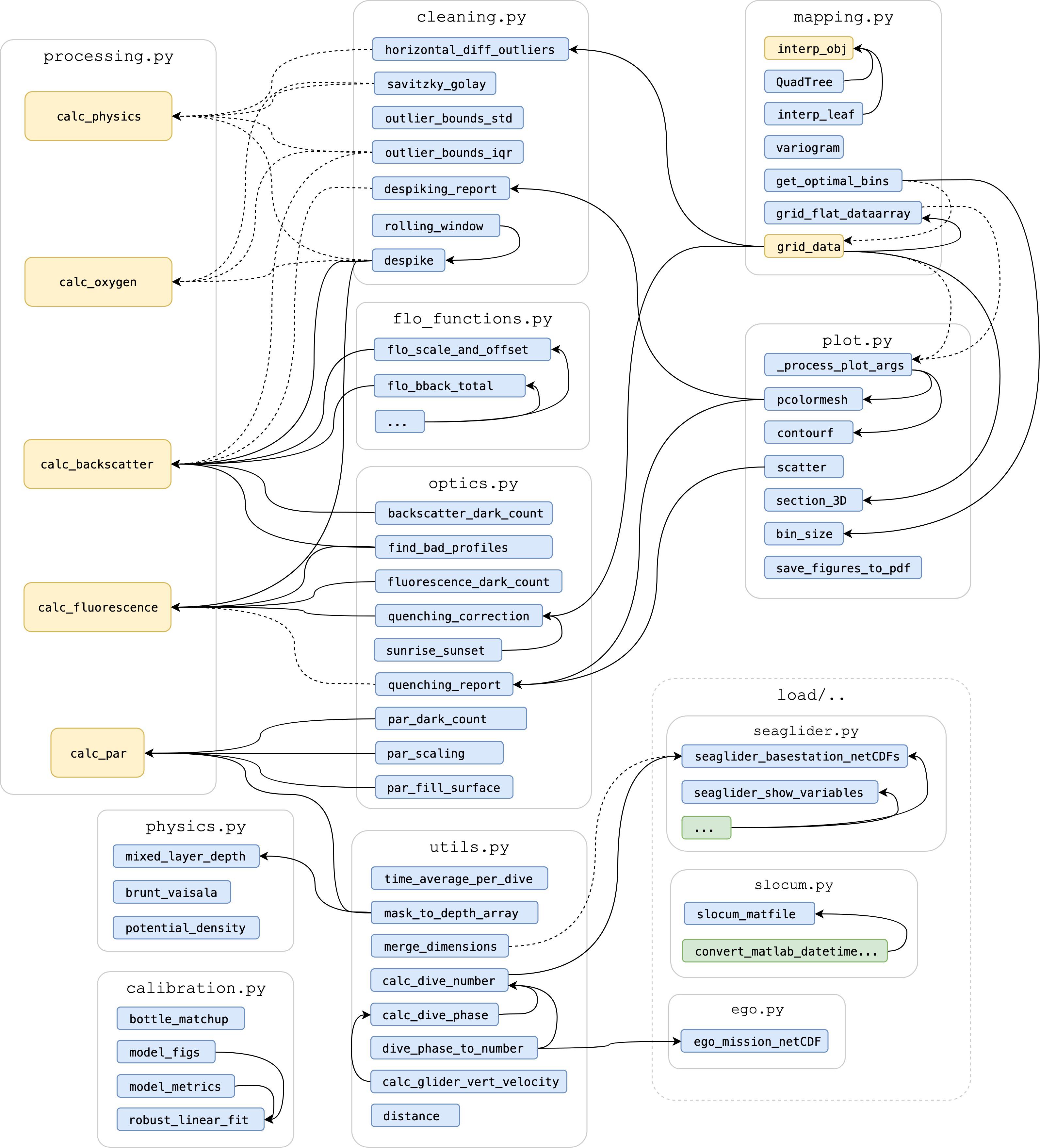
Figure 1. Package structure of GliderTools with arrows showing function calls, where solid lines show dependencies that are always called by a function and dashed lines show functions that are only called when specified by the user. Blue rectangles are nested functions in a python module (as grouped by gray boxes e.g., cleaning.py). Green rectangles are functions hidden from the user, while yellow functions are accessible to the user under the main GliderTools namespace. Note that some functions are simplified for brevity (e.g., seaglider.py).

FIGURE 2

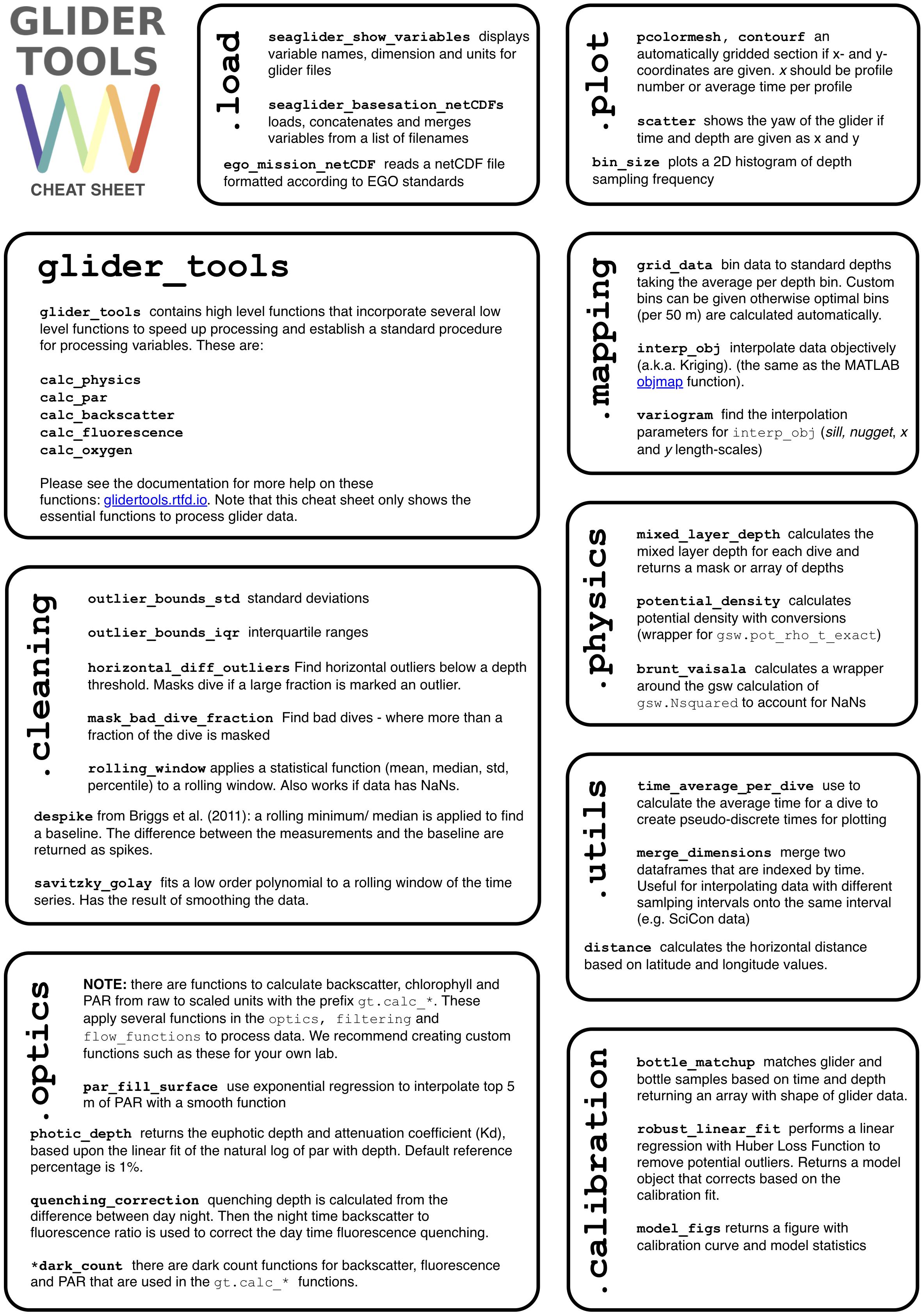
Figure 2. The GliderTools “cheat sheet,” a quick reference guide to using and implementing the tool. The boxes represent the various modules within the package. Details for each of these functions can be found in the online documentation (glidertools.readthedocs.org/).

We have provided functions under the gt.load module to explore and import data that are EGO-formatted netCDF files or have been processed by the Seaglider^TM base-station software. For the latter, loading data has been automated as much as possible, with coordinate variables, specifically time, being imported with associated variables to ensure that variables can be joined based on the sampling timestamp. While we focus on the Seaglider platform, there is room for other platforms (e.g., Slocum glider and other profiling platforms) to be incorporated, provided that the output is in a concatenated format.

Once in the standard concatenated format, any function can be applied to the data. GliderTools provides five high-level functions that automatically implement cleaning, calibration and correction procedures by applying the appropriate low-level functions in the sequence used by the SOCCO group (Figure 1). These high-level functions have a calc prefix followed by the variable name, e.g., gt.calc_backscatter.

The gt.cleaning module provides functions to filter erroneous data, remove spikes (when applicable) and smooth data once bad measurements and profiles have been removed. The tools were designed to be as objective as possible by finding thresholds from data vertically along the time axis, horizontally comparing dives, or globally considering all values. These tools can be applied to any profiled variable in any particular order. A data density filter (based on a two-dimensional histogram) can be applied to the data for any two variables (e.g., temperature and salinity), but values have to be tailored by the user for the specific case, making the tool a subjective approach.

GliderTools incorporates a gt.physics module to calculate derived physical variables, allowing users to calculate mixed-layer depth (MLD), potential density and the Brunt Väisälä frequency. The latter two functions use the Gibbs Seawater (GSW) toolbox with the added convenience to format output to match the input data and ensuring the use of absolute salinity and potential temperature when calculating potential density (McDougall and Barker, 2011).

The gt.optics module contains functions to process photosynthetically available radiation (PAR), backscatter, and fluorescence. The module provides functions to scale these variables from raw counts or voltages to factory calibrated units and perform in situ dark count corrections on each variable. Backscatter corrections are made using the methodology of Zhang et al. (2009) which is implemented in the flo_functions tools by the Ocean Observatory Initiative (Copyright© 2010, 2011 The Regents of the University of California; used under a free license). Further individual corrections to PAR, backscatter and fluorescence will be discussed in the following section. Notably, the gt.optics module also contains an updated version of the quenching correction method described by Thomalla et al. (2018), where corrections are now possible without PAR.

General utilities to process glider data are stored in the gt.utils module and include functions to merge datasets sampled at different intervals or manually define up and down dives or dive phase (as defined by the EGO gliders data management team, 2017). T can be applied automatically on import.

The gt.mapping module allows users to grid data in discrete bins or interpolate data two-dimensionally. The default bin sizes are based on the sampling frequency of the data to minimize the aliasing per depth bin in the gt.mapping.grid_data function. Alternatively, depth bins can be defined manually. The function can also be used to calculate any other aggregated statistical value; e.g., show the standard deviation per bin. Data can also be interpolated along any two dimensions with an objective mapping method (based on gt.mapping.objmap⁶). Note that the objmap and grid_data functions have been made available under the main namespace (as shown in Figure 1).

Lastly, the gt.plot module is designed to quickly represent gridded or ungridded data in a section format. The capability of this module will be demonstrated throughout this manual.

Workflow Examples

In this section, we have selected four examples that showcase the capability and methods of GliderTools. We first introduce the data we use in the examples. We then look at the secondary QC or cleaning functions that are available for, but not limited to physics data. The third part shows how raw fluorescence units are cleaned and converted to chlorophyll concentrations using bottle calibrations. In part four, we show how PAR is corrected and euphotic depth is calculated. Lastly, see section “Vertical Binning and Two-Dimensional Interpolation” shows how data is gridded vertically or interpolated over the vertical and horizontal dimensions.

Example Glider Dataset

The data represented here was collected from a Seaglider deployed in the South Atlantic sub-Antarctic region (43°S, 8.52°E) as part of the third Southern Ocean Seasonal Cycle Experiment (SOSCEx III; Swart et al., 2012; du Plessis et al., 2019). Seaglider (SG) 542 was deployed on 8th December 2015 and retrieved on 8th February 2016. A total of 344 dives are used in the example dataset containing data on temperature, conductivity, pressure, fluorescence, dissolved oxygen; PAR. The raw glider engineering and log files have undergone Kongsberg Basestation processing in which raw data is initially processed and quality controlled upon the glider data being received by the land-based server. The automated QC is done according to procedures modeled after the Argo data processing scheme (Schmid et al., 2007). The Basestation software returns netCDF formatted files for each dive. In this study, GliderTools applies processing on this netCDF output. Data are available at ftp://socco.chpc.ac.za/GliderTools/SOSCEx3.

Secondary QC for Physics Data: Filters and Smoothing

The gt.cleaning module offers methods that can either filter out erroneous data or smooth noisy data. The package provides three filters to remove outliers which we discuss briefly. Both gt.cleaning.outlier_bounds_iqr and gt.cleaning.outlier_bounds_std are global filters that remove outliers by interquartile and standard deviation limits, respectively. gt.cleaning.horizontal_diff_outliers compares horizontal adjacent values, masking a dive when a specified number of measurements exceed a threshold – data are automatically gridded to achieve this but the function returns the results as ungridded data. More details about these filters can be found in the online documentation.

The package includes three different smoothing procedures which are described below. We show the effect that smoothing has on an individual profile and suggest cases where these smoothing functions can be used. We have chosen a salinity profile (140.5, i.e., the up-cast) that demonstrates the effect of these smoothing functions. Note that these functions are applied along the time dimension.

1. The gt.cleaning.despike function is an adaptation of the approach used by Briggs et al. (2011) to remove spikes in backscatter data with the intention of preserving these points. In the case of optics variables, it is often the case that spikes are not erroneous data, but particles that could be used to calculate downward flux or export (Briggs et al., 2011). This is achieved by applying a rolling minimum window, followed by a rolling maximum window over the data. This extracts the baseline, with the residuals being returned as spikes. This filter is useful for data where the sampling noise is not normally distributed but rather positively distributed. The application to salinity (Figure 3) is thus only for demonstration and should not be applied in practice. A median filter can also be applied when it is expected that spikes are normally distributed. This produces a similar outcome to a rolling window over which a median function is applied.

2. gt.cleaning.rolling_window allows any aggregating function (mean, median, standard deviation, percentile) to be applied to the data allowing users to create further filters if needed. However, the tool can also be used to simply smooth data with mean or median functions.

3. Lastly, gt.cleaning.savitzky_golay fits a polynomial function to a rolling window of the data (Savitzky and Golay, 1964). The order of the polynomial can be determined by the user, thus more complex curves can be fit by the curve while smoothing the data.

Here, these three filters are applied individually to the raw profile (Figure 3), but these methods can be applied sequentially if required. We show that the despiking method has the largest impact on the data, with the selected minimum baseline clearly shown, with all spikes being positive. The Savitzky-Golay function and the rolling average window have similar effects on the profile with the latter having a stronger effect to smooth the data. The Savitzky-Golay method keeps the profile shape while removing high-frequency spikes in the data.

FIGURE 3

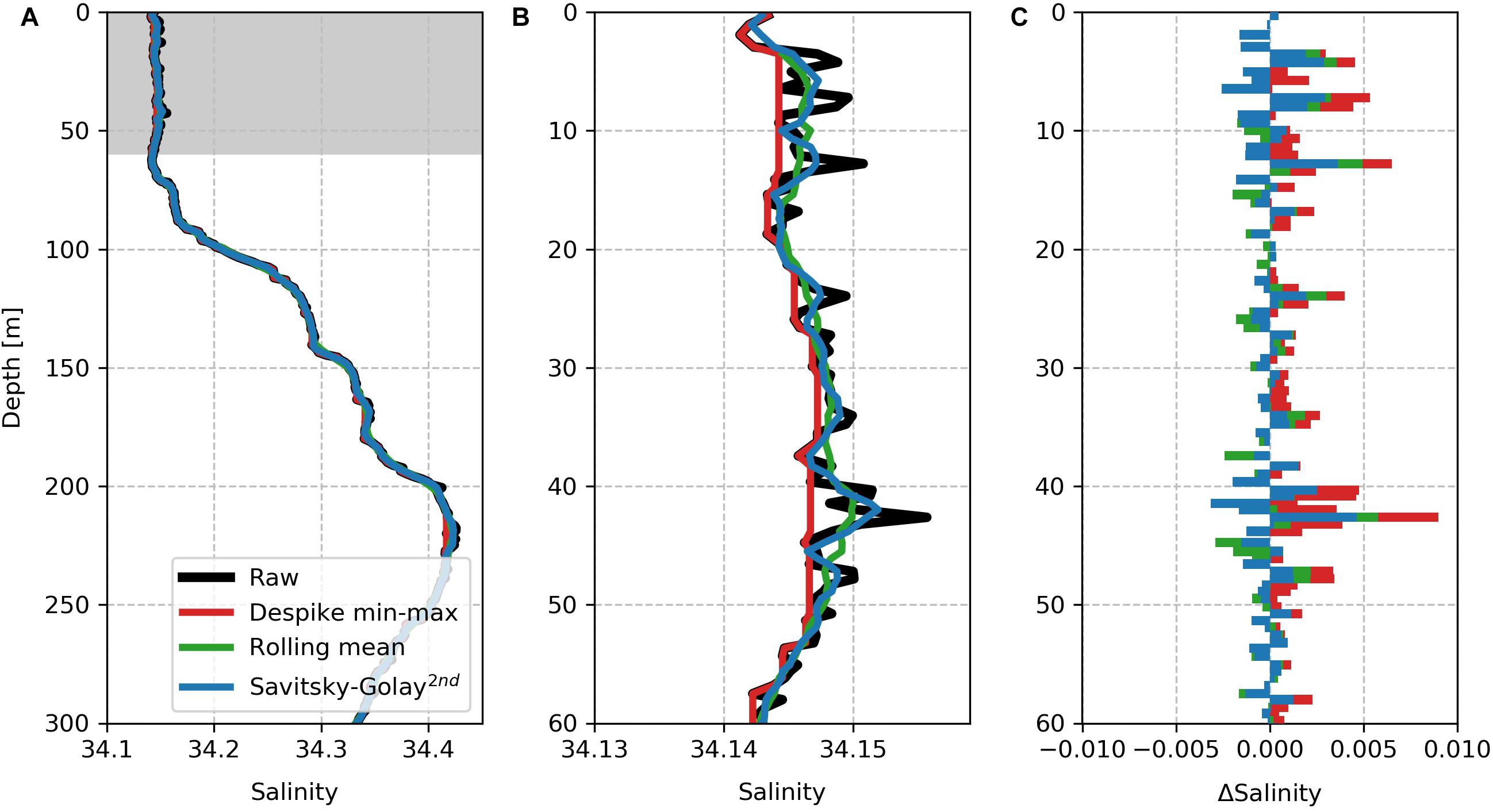
Figure 3. A comparison of the impact of the smoothing functions on a “noisy” part of profile 140.5 (up-cast). Note that a 9-point rolling window is applied in all cases. (A) A single depth profile of raw salinity in black overlaid by three cleaning methods applied to the raw salinity, namely despiked (red) with a rolling min-max window, rolling average (green) and second-order Savitzky-Golay smoothing (blue). The gray shading marks the region of the profile that is enlarged in panel (B). (C) The difference between the cleaned and raw salinity for each of the applied functions.

Fluorescence QC and Calibration

Fluorescence data provides useful information on phytoplankton biomass and bloom phenology, however, in vivo fluorescence is suppressed during periods of high irradiance due to a process termed non-photochemical quenching (Yentsch and Ryther, 1957; Slovacek and Hannan, 1977; Owens et al., 1980; Abbott et al., 1982; Falkowski and Kolber, 1995; Milligan et al., 2012). The ability to correct this has been successfully demonstrated, where GliderTools uses the method proposed in Thomalla et al. (2018). The full procedure including the cleaning steps is described below.

1. Raw fluorescence data is processed as follows:

a. Bad fluorescence profiles are identified with gt.optics.find_bad_profiles. Using a reference depth of 300 m, fluorescence is averaged below 300 m and profiles identified as outliers, where their depth specific values are greater than the global mean profile multiplied by a user defined value (e.g., a factor of 3).

b. An in situ dark-count is calculated with gt.optics.fluorescence_dark_count. The dark count is calculated from the 95th percentile between 300 and 400 m and then removed from the data.

c. The data is despiked using gt.cleaning.despike (the function described in see section “Secondary QC for Physics Data: Filters and Smoothing”) where an 11-point rolling minimum is applied to the dataset. Thereafter an 11-point rolling maximum is applied. This forms the baseline, where the spikes are the difference from the baseline.

d. Quenched data is corrected using gt.optics.quenching_correction, as described in Thomalla et al. (2018) and shown in Figures 4A,B.

i. The quenching depth is determined as the minimum depth of the five smallest differences between daytime fluorescence and average night-time fluorescence.

ii. The night-time backscattering ratio to fluorescence is used to correct the daytime fluorescence profile.

iii. The current method is set to use the night before (night_day_group = False) but can use the night after (night_day_group = True).

iv. Daytime is defined as local sunrise and sunset, using gt.optics.sunset_sunrise, with the addition of the sunrise_sunset_offset, which is defined as 2 h here.

2. Fluorescence data is converted into chlorophyll as follows:

a. The calibration data is matched to the glider within user-defined limits of 5 m in the depth dimension and 120 min in the time dimension. Note that the bottle calibration function (gt.calibration.bottle_matchup) does not take longitude and latitude into consideration, therefore the user must use only bottle samples that coincide with the glider data.

b. A Huber Linear Regression algorithm is applied to the matched bottle data. Huber regression is more robust than standard linear regression as outliers can be excluded from the fit based on a user-selected threshold (epsilon, 1.5 in this case). Additionally, for fluorescence, the y-intercept is forced to zero (Figure 4C).

c. This equation is then applied to the glider fluorescence to produce glider chlorophyll (mg m^–3) (Figure 4D).

FIGURE 4

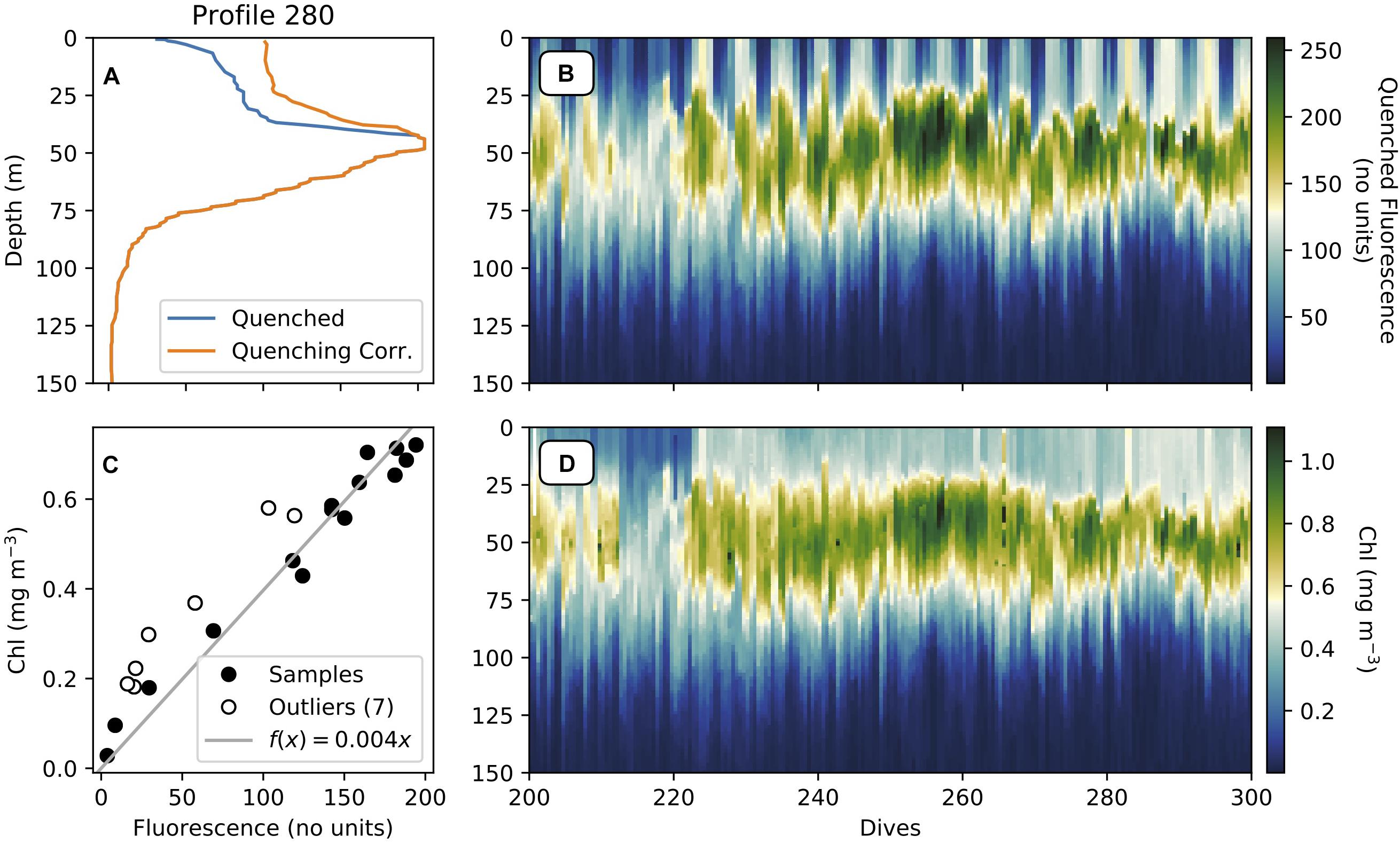
Figure 4. (A) Depth profiles of quenched and quenching-corrected fluorescence (unitless raw count), (B) Section plot of quenched fluorescence (no units), (C) Huber linear regression of glider fluorescence (no units) and in situ chlorophyll-a (mg m^–3), and (D) section of glider chlorophyll (mg m^–3).

PAR Quality Control and Derivations

Photosynthetically available radiation data provides valuable information on the photic environment of the surface ocean – key to understanding the phytoplankton light status, including the derivation of the euphotic zone thickness (euphotic depth) and the diffuse attenuation coefficient (k_d). The accurate characterization of the photic environment is important if this data is to be integrated into primary production models. The processing steps for PAR within GliderTools are discussed below.

1. Raw PAR data is processed as follows:

a. PAR (μV) is scaled to μE m^–2 s^–1 and corrected for factory dark count (gt.optics.par_scaling).

b. PAR is corrected for an in situ dark-count using gt.optics.par_dark_count (median PAR value at night, values excluded before 23:01 local time and outside the 90th percentile).

c. Top 5 m is removed and then the profile is algebraically recalculated using an exponential equation using gt.optics.par_fill_surface (Figures 5A,B).

2. The euphotic depth and k_d can be calculated from this corrected PAR using gt.optics.photic_depth.

a. Euphotic depth defined as 1% of surface PAR (Figure 5C).

b. k_d defined as the slope of the linear fit of depth and ln(PAR) (Figure 5D).

FIGURE 5

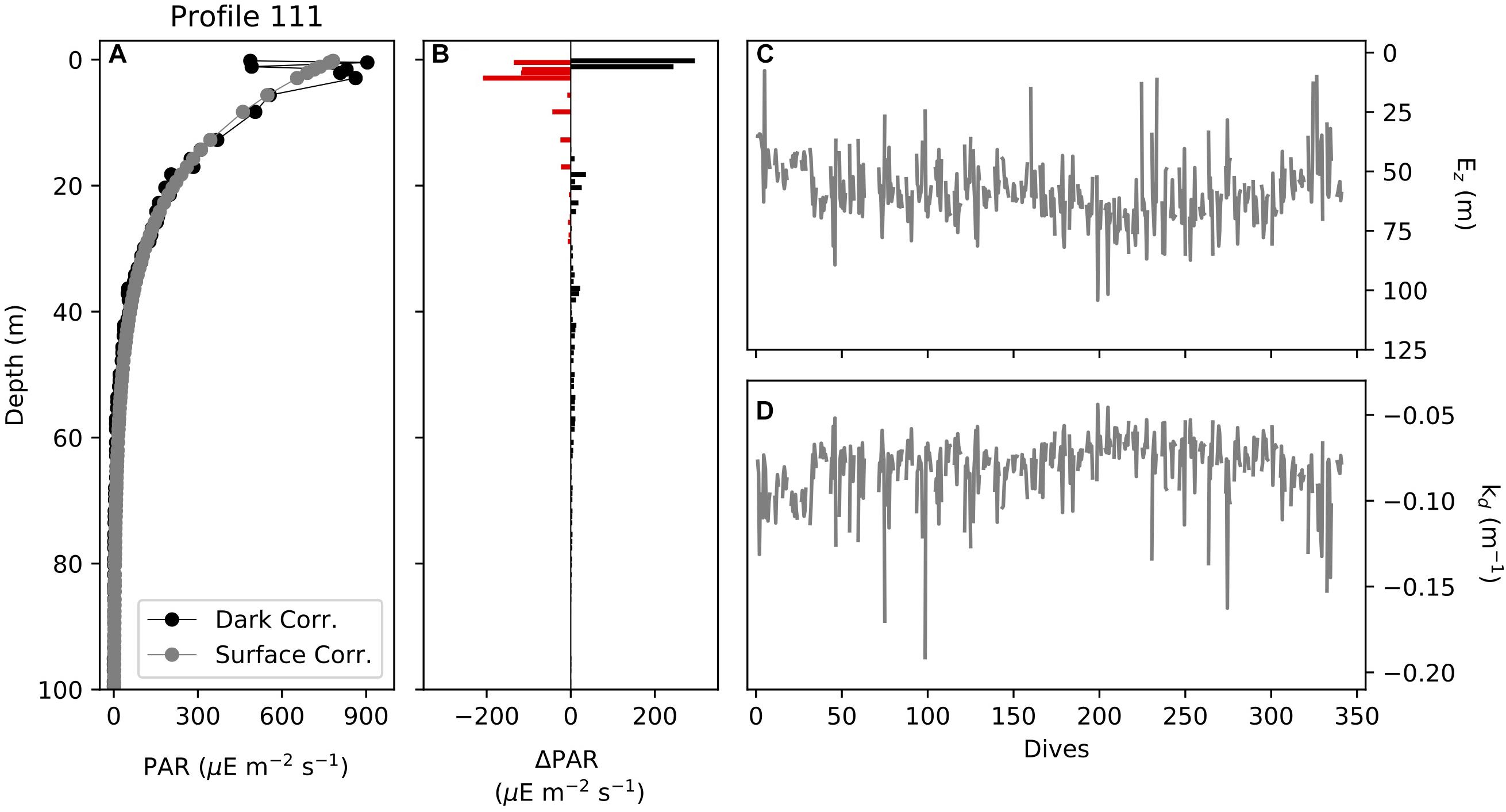
Figure 5. (A) Profiles of dark corrected (factory and in situ dark corrected) PAR (μE m^–2 s^–1) and surface corrected PAR (algebraic correction), (B) the difference between dark corrected and surface corrected PAR, (C) the euphotic depth (m) calculated from PAR for the glider section and (D) the diffuse attenuation coefficient, k_d, (m^–1) calculated from PAR for the glider section.

Vertical Binning and Two-Dimensional Interpolation

Throughout the cleaning and calibration processing, GliderTools prioritizes maintaining the structure of the data, i.e., data are not gridded. However, it is often more convenient, computationally efficient and required for certain calculations to work with data that is on a regular grid. GliderTools offers two methods to place data on a regular grid. The first is by binning only the vertical coordinate of the data. The second approach is a two-dimensional optimal interpolation. The processing and additional information are discussed in the steps below.

1. Vertical data binning is described below:

a. The vertical binning procedure of GliderTools (gt.grid_data) requires a pseudo-discrete x-coordinate. The profile number can typically be used, but there is also a function to calculate the average time stamp for each profile (gt.utils.time_average_per_dive).

b. If vertical gridding bins are not defined manually gt.grid_data automatically assigns bins according to the average sampling density per 50 m, as demonstrated in Figure 6A with the gridded output shown in Figure 6C. The bins are rounded up to the nearest 0.5 m, meaning that “full” bins are preferred over “sparse” bins. Binning data at the optimal sampling frequency is important if the user wants to preserve as much of the vertical structure as possible without creating a sparse dataset. It becomes clear that the lack of horizontal interpolation becomes limiting, with the discrete bins clearly visible in the zoomed in section.

2. Two-dimensional interpolation is perhaps a better approach when, for example, comparing gradients over shorter time-scales. Past studies have used a MATLAB implementation of objective mapping (objmap in the MATLAB toolbox⁷, Thompson et al., 2016; Todd et al., 2016; Viglione et al., 2018; du Plessis et al., 2019). GliderTools offers a Pythonic implementation of the MATLAB objective interpolation function (gt.interp_obj). Because of its statistical foundation, objective mapping is also able to calculate interpolation errors. In practice, objective mapping is a form of inverse distance weighted interpolation, where the weight of observations decreases as calculated by a radial kernel (Gaussian in this case). However, calculating the weights of the model does not scale well computationally due to large memory requirements. The problem is thus broken into smaller, parallelizable subsets using a quadtree approach and interpolation is performed for each quadrant and its neighbors.

a. As with vertical gridding, an interpolation grid has to be created for the interpolation. GliderTools does not offer assistance in deciding on the size and frequency of this grid. The demonstration below uses a 1 m vertical grid with a 30-min horizontal grid. Details on how these are created are in the online documentation.

b. The user must manually estimate the anisotropy of the horizontal and vertical length-scales of the coordinates. This can be determined using a variogram (gt.mapping.variogram, Figure 6E); however, we find that manual estimates of the length scales often result in better interpolation, especially when interpolating data over the thermocline. The variogram function automatically scales the x and y coordinates so that the range is one. This means that the user only needs to find the anisotropy (ratio between x and y length scales). It may also be helpful to mask out the deeper, homogeneous parts of the section to estimate the more variable length scales in the surface waters. The variogram function is also used to find the nugget (error estimate of sampling) and sill (maximum semivariance of the model). The following have been used in Figure 6E: 70 m in the vertical and 60 h on the horizontal; a partial sill of 0.02 (sill – nugget) and a nugget of 0.004.

c. As mentioned, the gt.interp_obj function can also calculate interpolation errors for a particular interpolation scheme. It is important to consider interpolation errors when there are large gaps in the dataset – as in the first few dives in Figures 6B,D. Regions with large errors can be used to mask regions with low interpolation confidence.

FIGURE 6

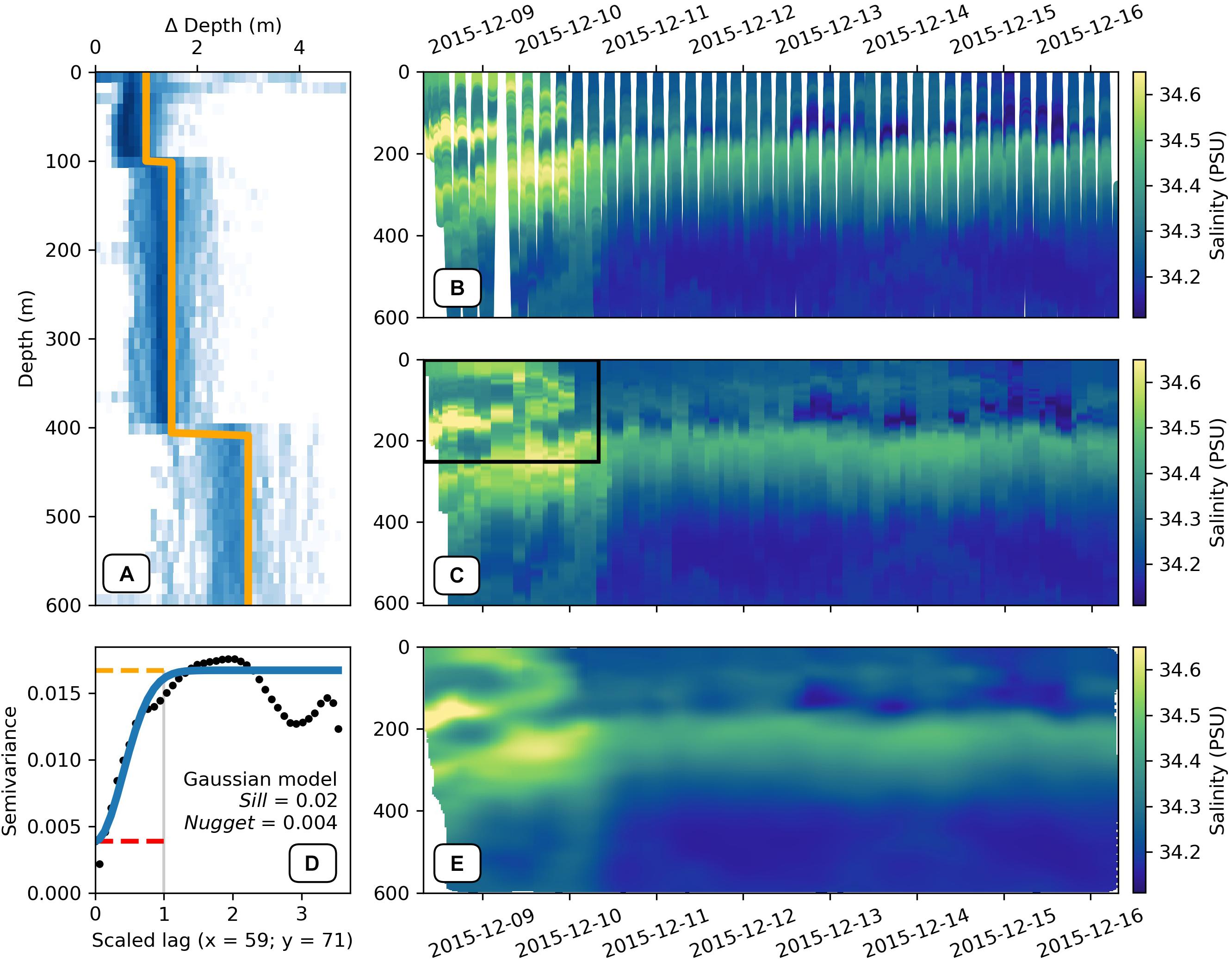
Figure 6. (A) A two-dimensional histogram of the vertical sampling frequency at various depths. The orange line shows the algorithmically estimated bin sizes for each 50 m block (median vertical sampling frequency rounded down to the nearest 0.5 m). (B) A scatter plot of ungridded salinity that has been quality controlled using the calc_physics function. (C) The salinity data from (B) gridded vertically according to the sampling frequencies shown in (A) with the average time per dive as the x-axis coordinate. The black box shows the subset of data that was used to calculate the semivariance in panel (D). (D) The semivariance (black dots) of salinity scaled anisotropically so that the range (gray) is equal to one. The blue line shows a gaussian model fit to the semivariance with the sill (orange) and nugget (red) shown by the dashed lines. (E) shows the objectively interpolated data using the sill (0.02), nugget (0.004) and coordinate length-scales (70 h and 60 m for x and y, respectively), from (D). Regions with large interpolation errors have been masked (nugget + 5% of nugget).

Discussion

Recommendations for Processing and Data Management

One of the advantages of GliderTools, in comparison to existing packages, is the ability to clean and despike the raw data, with complete user control of the strict QC procedure. This is important when cleaning physics data in comparison to cleaning bio-optical data. A spike in either the salinity or temperature is more than likely a technical failure of the sensor i.e., power surges, whereas a spike in either the backscatter or fluorescence is aggregated biological matter, i.e., marine snow or fecal pellets (Fischer et al., 1996; Bishop et al., 1999; Gardner et al., 2000; Bishop and Wood, 2008). Thomalla et al. (2018) built upon the work of Briggs et al. (2011) to distinguish spikes from both backscatter and fluorescence sensors in order to develop a new optimized approach for correcting fluorescence quenching. This approach was required as large spikes in the backscatter data would significantly alter the fluorescence to backscatter ratio, invalidating their approach of using the nighttime ratio to correct daytime quenching. Whilst the technique of removing spikes is appropriate for correcting quenched fluorescence, it does not hold true for estimating carbon flux and export from backscatter. As such, GliderTools removes the spikes to accurately correct fluorescence quenching but it also retains the spikes as a variable that can be reincorporated back into the backscatter.

For the calculation of vertical and horizontal (temporal and spatial) gradients of physical properties in the ocean, GliderTools performs optimal interpolation/objective mapping to the raw data, providing data gridded to a monotonically increasing grid. This approach is particularly useful for studies investigating the evolution of submeso- to mesoscale processes (Thompson et al., 2016; Todd et al., 2016; Viglione et al., 2018; du Plessis et al., 2019) as it negates the bias in the calculation which may arise due to non-uniform horizontal gridding. Note this does not remove the challenge of distinguishing variations in the given property as spatial or temporal, or some combination of these, but provides the user with robust method of along-track interpolation which is currently only available in a MATLAB implementation.

GliderTools encourages best practices in terms of post-data collection efforts in data distribution, storage and open-source, which is detailed further in Testor et al. (2019). GliderTools has implemented, where possible, best practise in terms of development and provision of metadata. We advocate for glider data storage and dissemination through regional and global data repositories (e.g., NCEI, PODAAC, BODC and discoverable through sites such as SOOSmap; Newman et al., 2019). GliderTools should continue to strive toward common glider data formatting and standardization in order to conform to the community agreed requirements (such as protocols and recommendations coming from OceanGliders). This will, of course, be an iterative process – i.e., when glider users and managers convene and provide guidelines on data management, including the implementation of Findable-Accessible-Interoperable-Reusable (FAIR) data principles. GliderTools’ open code viewpoint will, therefore, facilitate best practise of data formatting and QC procedures to evolve and keep up-to-date with internationally agreed practices. The rapid acceleration of glider use by the research and operational community means that coordination and standardization will become an ever-important aspect for glider data in the coming years.

Limitations and Potential Developments

In the development of GliderTools, we have attempted to provide a package that addresses our own needs and thus recognize that it will not be comprehensive for each and every user. However, we encourage the community-driven development of packages that incorporate or integrate with GliderTools.

Perhaps the clearest limitation is the lack of support for multiple glider platforms, e.g., the Slocum glider by Teledyne Marine⁸ and the Spray glider by Bluefin Robotics⁹. At its core, GliderTools was written to support head-to-tail concatenated column data, thus making the addition of platform-specific functions simple (though we recommend the use of xarray to make full use of metadata preservation in GliderTools). The glider community (EGO – Everyone’s Glider Observations) is making a concerted effort to standardize data processing and storage to streamline access of first-order processed data. GliderTools thus includes a function to load this community standard netCDF format. Improving the support for other data formats will likely be the next step forward in the development of GliderTools.

The presence of thermal lag in conductivity data can introduce false signals in salinity and density, especially at the thermocline, thus the absence of thermal lag correction function in GliderTools may be perceived as a shortcoming. However, this problem has been addressed to various degrees by the Basestation, SOCIB and UEA glider packages. In principle, these packages model the glider speed through the water to apply a temporal lag correction to conductivity relative to temperature measurements (Garau et al., 2011). We encourage the creators of the thermal lag correction functions to produce a Python implementation of the corrections that could be implemented into GliderTools.

Continuing work has shown that open and coastal ocean oxygen concentrations have decreased due to the imprint left in the atmosphere due to fossil fuel burning and eutrophication (Breitburg et al., 2018). Gliders are thus often fitted with oxygen sensors (e.g., Aanderaa oxygen optodes) to measure these important changes (Bittig et al., 2018; Queste et al., 2018). In its current state, GilderTools offers only data filtering, smoothing, unit conversion and the calculation of theoretical oxygen saturation and apparent oxygen utilization. Bittig et al. (2018) present a comprehensive overview of best practices in dissolved oxygen processing, which should be used as a guideline for the development of more comprehensive oxygen processing. We thus invite the community to contribute to the development of tools to process glider measured variables currently not supported by GliderTools (see the contribution guidelines in our code repository).

The quenching correction of Thomalla et al. (2018) implemented in GliderTools is created and tested for open-ocean waters and thus cannot be applied with confidence to glider data collected in coastal waters. The approach assumes that all backscatter is due to biological material – the backscatter of sedimentary material in coastal and shelf waters invalidates this. Future fluorescence quenching correction methods will need to be developed to specifically handle data from coastal and shelf regions and we hope these to be incorporated into GliderTools in time.

Further, the current approach of estimating chlorophyll from a linear relationship with fluorescence is based upon two assumptions, that sensor excitation energy is constant, and saturating and that chlorophyll absorption and fluorescence quantum yield are linearly related to fluorescence. This is not always the case in situ due to pigment packaging, cell size, community structure, light history and nutritional status. In recent studies, Haëntjens et al. (2017) and Johnson et al. (2017) used a power-law regression between high-performance liquid chromatography estimated chlorophyll-a and profiling float fluorescence, which reduced the errors and improved the correlation coefficient. The current approach provided within GliderTools requires the user to not fit the intercept as doing so will result in anomalously high (∼0.1 mg m^–3) chlorophyll values at depth (>200 m); a power-law approach will not require this assumption to be made.

Conclusion

We present GliderTools, an open-source Python software package for processing underwater glider data for scientific use. Previously available packages are focussed on processing raw glider output, usually limited to only temperature and salinity data and are, in many cases, reliant on proprietary scientific programing languages. The tools we provide will allow users to focus more on the science by removing the barrier of technical programing. This barrier is further reduced with the high-level functions we provide for more complex variables such as backscatter and fluorescence, that apply multiple processing steps.

Lastly, GliderTools was developed to address the needs of the research groups involved in this study and thus, we recognize that it will not address the needs of all scientists using glider data. We invite other users to suggest improvements and contribute toward the further development of the tool. We also encourage users to contribute to or suggest changes toward the documentation of GliderTools, which is key to the usability of the package. With GliderTools we advocate that as the glider community moves toward open-source data, so should the programs that handle and process the data.

Data Availability Statement

The datasets for this study can be found in the SOCCO data server at ftp://socco.chpc.ac.za/GliderTools/SOSCEx3.

Author Contributions

LG conceptualized the manuscript and was the primary contributor to the code for the GliderTools package. TR-K wrote the majority of the code and text relating to bio-optics. S-AN, MP, and IG contributed to the conceptual development and testing of GliderTools as well as writing the manuscript. SS contributed to the manuscript as well as the addition of certain functions to GliderTools. All authors revised and approved the manuscript.

Funding

Initial development of this project was funded by the NRF-SANAP Grant SNA170524232726. SS acknowledges support from a Wallenberg Academy Fellowship (WAF 2015.0186). S-AN acknowledges the CSIR Parliamentary Grant, Young Researchers Establishment Fund (YREF 2019 0000007361). S-AN and SS were supported by the NRF-SANAP Grant SNA170522231782.

Conflict of Interest

The authors declare that the research was conducted in the absence of any commercial or financial relationships that could be construed as a potential conflict of interest.

Acknowledgments

We would like to acknowledge Christopher Wingard, Craig Risien, and Russell Desiderio for the use of the flo_functions package. LG was employed by the ETH Zürich during manuscript preparation and would like to thank the group leader, Nicolas Gruber, for allowing time to complete this project. We would like to thank Pedro Monteiro for supporting the initial code development. We thank SANAP and the captain and crew of the S. A. Agulhas II for their assistance in the deployment and retrieval of gliders used to obtain the data for this paper. We also acknowledge the work of STS for housing, managing, and piloting the gliders and for the IOP hosting provided by Geoff Shilling and Craig Lee of the Applied Physics Laboratory, University of Washington.

Footnotes

1. ^ https://podaac.jpl.nasa.gov
2. ^ https://www.nodc.noaa.gov
3. ^ https://gliders.ioos.us
4. ^ http://www.ifremer.fr/co/ego/ego/v2/
5. ^ http://www.byqueste.com/toolbox.html
6. ^ http://mooring.ucsd.edu/index.html?/software/matlab/matlab_intro.html
7. ^ http://mooring.ucsd.edu/software/matlab/doc/toolbox/
8. ^ http://www.teledynemarine.com/slocum-glider
9. ^ https://auvac.org/platforms/view/120

References

Abbott, M. R., Richerson, P. J., and Powell, T. M. (1982). In situ response of phytoplankton fluorescence to rapid variations in light. Limnol. Oceanogr. 27, 218–225. doi: 10.4319/lo.1982.27.2.0218

CrossRef Full Text | Google Scholar

Bishop, J. K. B., and Wood, T. J. (2008). Particulate matter chemistry and dynamics in the twilight zone at VERTIGO ALOHA and K2 sites. Deep Sea Res. Part I 55, 1684–1706. doi: 10.1016/j.dsr.2008.07.012

CrossRef Full Text | Google Scholar

Bishop, K. B. J., Calvert, S. E., and Soon, M. Y. S. (1999). Spatial and temporal variability of POC in the northeast subarctic Pacific. Deep Sea Res. Part II 46, 2699–2733. doi: 10.1016/S0967-0645(99)00081-8

CrossRef Full Text | Google Scholar

Bittig, H. C., Körtzinger, A., Neill, C., van Ooijen, E., Plant, J. N., Hahn, J., et al. (2018). Oxygen optode sensors: principle, characterization, calibration, and application in the ocean. Front. Mar. Sci. 4:429. doi: 10.3389/fmars.2017.00429

CrossRef Full Text | Google Scholar

Breitburg, D., Levin, L. A., Oschlies, A., Grégoire, M., Chavez, F. P., Conley, D. J., et al. (2018). Declining oxygen in the global ocean and coastal waters. Science 359:eaam7240. doi: 10.1126/science.aam7240

PubMed Abstract | CrossRef Full Text | Google Scholar

Briggs, N., Perry, M. J., Cetinić, I., Lee, C., D’Asaro, E., Gray, A. M., et al. (2011). High-resolution observations of aggregate flux during a sub-polar North Atlantic spring bloom. Deep Sea Res. Part I 58, 1031–1039. doi: 10.1016/j.dsr.2011.07.007

CrossRef Full Text | Google Scholar

du Plessis, M., Swart, S., Ansorge, I. J., Mahadevan, A., and Thompson, A. F. (2019). Southern ocean seasonal restratification delayed by submesoscale wind–front interactions. J. Phys. Oceanogr. 49, 1035–1053. doi: 10.1175/jpo-d-18-0136.1

CrossRef Full Text | Google Scholar

EGO gliders data management team, (2017). in EGO Gliders NetCDF Format Reference Manual, eds T. Carval, C. Gourcuff, J.-P. Rannou, J. J. H. Buck, and B. Garau, Paris: Ifremer, doi: 10.13155/34980

CrossRef Full Text | Google Scholar

Falkowski, Z., and Kolber, P. G. (1995). Variations in Chlorophyll fluorescence yields in phytoplankton in the World Oceans. Aust. J. Plant Physiol. 22, 341–355.

Google Scholar

Fernandes, F. (2014). python-seawater v3.3.2. Switzerland: Zenodo, doi: 10.5281/zenodo.11395

CrossRef Full Text | Google Scholar

Fischer, G., Neuer, S., Wefer, G., and Krause, G. (1996). Short-term sedimentation pulses recorded with a chlorophyll sensor and sediment traps in 900 m water depth in the Canary Basin. Limnol. Oceanogr. 41, 1354–1359. doi: 10.4319/lo.1996.41.6.1354

CrossRef Full Text | Google Scholar

Garau, B., Ruiz, S., Zhang, W. G., Pascual, A., Heslop, E., Kerfoot, J., et al. (2011). Thermal lag correction on slocum CTD glider data. J. Atmos. Ocean. Technol. 28, 1065–1071. doi: 10.1175/JTECH-D-10-05030.1

CrossRef Full Text | Google Scholar

Gardner, W. D., Richardson, M. J., and Smith, W. O. (2000). Seasonal patterns of water column particulate organic carbon and fluxes in the ross sea, antarctica. Deep-Sea Res. Part II 47, 3423–3449. doi: 10.1016/S0967-0645(00)00074-6

CrossRef Full Text | Google Scholar

Haëntjens, N., Boss, E., and Talley, L. D. (2017). Revisiting Ocean Color algorithms for chlorophyll a and particulate organic carbon in the Southern Ocean using biogeochemical floats. J. Geophys. Res. 122, 6583–6593. doi: 10.1002/2017JC012844

CrossRef Full Text | Google Scholar

Hoyer, S., and Hamman, J. J. (2017). xarray: N-D labeled arrays and datasets in python. J. Open Res. Softw. 5, 1–6. doi: 10.5334/jors.148

CrossRef Full Text | Google Scholar

Hunter, J. D. (2007). Matplotlib: a 2D graphics environment. Comput. Sci. Eng. 9, 99–104. doi: 10.1109/MCSE.2007.55

CrossRef Full Text | Google Scholar

Johnson, K. S., Plant, J. N., Coletti, L. J., Jannasch, H. W., Sakamoto, C. M., Riser, S. C., et al. (2017). Biogeochemical sensor performance in the SOCCOM profiling float array. J. Geophys. Res. 122, 6416–6436. doi: 10.1002/2017JC012838

CrossRef Full Text | Google Scholar

Jones, E., Oliphant, T., and Peterson, P. (2001). SciPy: Open Source Scientific Tools for Python. Available at: http://www.scipy.org/

Google Scholar

McDougall, T. J., and Barker, P. M. (2011). Getting started with TEOS-10 and the Gibbs Seawater (GSW) Oceanographic Toolbox, 28 SCOR/IAPSO WG127. Available at: www.TEOS-10.org (accessed February 04, 2018).

Google Scholar

Mckinney, W. (2010). “Data structures for statistical computing in python,” in Proceedings of the 9th Python in Science Conference, 1697900(Scipy), 51, Austin.

Google Scholar

Milligan, A. J., Aparicio, U. A., and Behrenfeld, M. J. (2012). Fluorescence and nonphotochemical quenching responses to simulated vertical mixing in the marine diatom Thalassiosira weissflogii. Mar. Ecol. Progr. Ser. 448, 67–78. doi: 10.3354/meps09544

CrossRef Full Text | Google Scholar

Newman, L., Heil, P., Trebilco, R., Katsumata, K., Constable, A., van Wijk, E., et al. (2019). Delivering sustained, coordinated, and integrated observations of the southern ocean for global impact. Front. Mar. Sci. 6:433. doi: 10.3389/fmars.2019.00433

CrossRef Full Text | Google Scholar

Owens, T. G., Falkowski, P. G., and Whitledge, T. E. (1980). Diel periodicity in cellular chlorophyll content in marine diatoms. Mar. Biol. 59, 71–77. doi: 10.1007/BF00405456

CrossRef Full Text | Google Scholar

Plotly Technologies Inc (2015). Collaborative Data Science. Montréal, QC: Plotly Technologies Inc.

Google Scholar

PyKrige Developers (2018). PyKrige: Kriging Toolkit for Python (Version 1.4.1) [Computer Software]. Available at: https://github.com/bsmurphy/PyKrige (accessed April 02, 2019).

Google Scholar

Queste, B. Y., Vic, C., Heywood, K. J., and Piontkovski, S. A. (2018). Physical controls on oxygen distribution and denitrification potential in the North West Arabian Sea. Geophys. Res. Lett. 45, 4143–4152. doi: 10.1029/2017GL076666

CrossRef Full Text | Google Scholar

Rudnick, D. L., Davis, R. E., Eriksen, C. C., Fratantoni, D. M., and Perry, M. J. (2004). Underwater gliders for ocean research. Mar. Technol. Soc. J. 38, 73–84. doi: 10.4031/002533204787522703

CrossRef Full Text | Google Scholar

Savitzky, A., and Golay, M. J. E. (1964). Smoothing and differentiation of data by simplified least squares procedures. Anal. Chem. 36, 1627–1639. doi: 10.1021/ac60214a047

PubMed Abstract | CrossRef Full Text | Google Scholar

Schmid, C., Molinari, R. L., Sabina, R., Daneshzadeh, Y. H., Xia, X., Forteza, E., et al. (2007). The real-time data management of system for argo profiling float observations. J. Atmos. Ocean. Technol. 24, 1608–1628. doi: 10.1175/JTECH2070.1

CrossRef Full Text | Google Scholar

Slovacek, R. E., and Hannan, P. J. (1977). In vivo fluorescence determinations of phytoplankton chlorophyll a. Limnol. Oceanogr. 22, 919–925. doi: 10.4319/lo.1977.22.5.0919

CrossRef Full Text | Google Scholar

Swart, S., Chang, N., Fauchereau, N., Joubert, W., Lucas, M., Mtshali, T., et al. (2012). Southern ocean seasonal cycle experiment 2012: seasonal scale climate and carbon cycle links. South Afr. J. Sci. 108, 3–5. doi: 10.4102/sajs.v108i3/4.1089

CrossRef Full Text | Google Scholar

Testor, P., Turpin, V., DeYoung, B., Rudnick, D. L., Glenn, S., Kohut, J., et al. (2019). OceanGliders: a component of the integrated GOOS. Front. Mar. Sci. 6:422. doi: 10.3389/fmars.2019.00422

CrossRef Full Text | Google Scholar

Thomalla, S. J., Moutier, W., Ryan-Keogh, T. J., Gregor, L., and Schütt, J. (2018). An optimized method for correcting fluorescence quenching using optical backscattering on autonomous platforms. Limnol. Oceanogr. 16, 132–144. doi: 10.1002/lom3.10234

CrossRef Full Text | Google Scholar

Thompson, A. F., Lazar, A., Buckingham, C., Naveira Garabato, A. C., Damerell, G. M., and Heywood, K. J. (2016). Open-ocean submesoscale motions: a full seasonal cycle of mixed layer instabilities from gliders. J. Phys. Oceanogr. 46, 1285–1307. doi: 10.1175/JPO-D-15-0170.1

CrossRef Full Text | Google Scholar

Todd, R. E., Owens, W. B., and Rudnick, D. L. (2016). Potential vorticity structure in the north atlantic western boundary current from underwater glider observations. J. Phys. Oceanogr. 46, 327–348. doi: 10.1175/jpo-d-15-0112.1

CrossRef Full Text | Google Scholar

Troupin, C., Beltran, J. P., Heslop, E., Torner, M., Garau, B., Allen, J., et al. (2015). A toolbox for glider data processing and management. Methods Oceanogr. 1, 13–23. doi: 10.1016/j.mio.2016.01.001

CrossRef Full Text | Google Scholar

Van Der Walt, S., Colbert, S. C., and Varoquaux, G. (2011). The NumPy array: a structure for efficient numerical computation. Comput. Sci. Eng. 13, 22–30. doi: 10.1109/MCSE.2011.37

CrossRef Full Text | Google Scholar

Viglione, G. A., Thompson, A. F., Flexas, M. M., Sprintall, J., and Swart, S. (2018). Abrupt transitions in submesoscale structure in southern drake passage: glider observations and model results. J. Phys. Oceanogr. 48, 2011–2027. doi: 10.1175/jpo-d-17-0192.1

CrossRef Full Text | Google Scholar

Yentsch, C. S., and Ryther, J. H. (1957). Short-term variations in phytoplankton and their significance. Limnol. Oceanogr. 2, 140–142. doi: 10.1111/gcb.14392

PubMed Abstract | CrossRef Full Text | Google Scholar

Zhang, X., Hu, L., and He, M. (2009). Scattering by pure seawater: effect of salinity. Optics Exp. 17:5698. doi: 10.1364/OE.17.005698

PubMed Abstract | CrossRef Full Text | Google Scholar